Two-step Sound Source Separation: Training on Learned Latent Targets

Abstract

In this paper, we propose a two-step training procedure for source separation via a deep neural network. In the first step we learn a transform (and it’s inverse) to a latent space where masking-based separation performance using oracles is optimal. For the second step, we train a separation module that operates on the previously learned space. In order to do so, we also make use of a scale-invariant signal to distortion ratio (SI-SDR) loss function that works in the latent space, and we prove that it lower-bounds the SI-SDR in the time domain. We run various sound separation experiments that show how this approach can obtain better performance as compared to systems that learn the transform and the separation module jointly. The proposed methodology is general enough to be applicable to a large class of neural network end-to-end separation systems.

Index Terms—  Audio source separation, signal representation, cost function, deep learning

1 Introduction

Single-channel audio source separation is a fundamental problem in audio analysis, where one extracts the individual sources that constitute a mixture signal [1]. Popular algorithms for source separation include independent component analysis [2], non-negative matrix factorization [3] and more recently supervised [4, 5, 6, 7, 8] and unsupervised [9, 10, 11] deep learning approaches. In many of the recent approaches, separation is performed by applying a mask on a latent representation, which is often a Fourier-based or a learned domain. Specifically, a separation module produces an estimated masked latent representation for the input sources and a decoder translates them back to the time domain.

Many approaches have used the short-time Fourier transform (STFT) as an encoder to obtain this latent representation, and conversely the inverse STFT (iSTFT) as a decoder. Using this representation, separation networks have been trained using a loss defined over various targets, such as: raw magnitude spectrogram representations [4], ideal STFT masks [12, 13] and ideal affinity matrices [5, 14]. Other works have supplemented this by additionally reconstructing the phase of the sources [8, 15]. However, the ideal STFT masks impose an upper bound on the separation performance the aforementioned criteria do not necessarily translate to optimal separation. In order to address this, recent works have proposed end-to-end separation schemes where the encoder, decoder and separation modules are jointly optimized using a time-domain loss between the reconstructed sources waveforms and their clean targets [7, 16, 17]. However, a joint time-domain end-to-end training approach might not always yield an optimal decomposition of the input mixtures resulting to worse performance than the fixed STFT bases [17].

Some studies have reported significant benefits when performing source-separation in two stages. In [18], first the sources are separated and in a second stage the interference between the estimated sources is reduced. Similarly, an iterative scheme is proposed in [17], where the separation estimates from the first network are used as input to the final separation network. In [19], speaker separation is performed by first separating frame-level spectral components of speakers and later sequentially grouping them using a clustering network. Lately, state-of-the-art results in most natural language processing tasks have been achieved by pre-training the encoder transformation network [20].

In this work, we propose a general two-step approach for performing source separation which can be used in any mask-based separation architecture. First we pre-train an encoder and decoder in order to learn a suitable latent representation. In the second step, we train a separation module using as loss the negative permutation invariant [21] scale invariant SDR (SI-SDR) [22] w.r.t. the learned latent representation. Moreover, we prove that for the case that the decoder is a transpose convolutional layer [7, 17], SI-SDR on the latent space bounds from below time-domain SI-SDR. Our experiments show that by maximizing SI-SDR on the learned latent targets, a consistent performance improvement is achieved across multiple sound separation tasks compared to the time-domain end-to-end training approach when using the exact same model architecture. The SI-SDR upper bound using the learned latent space is also significantly higher than that of STFT-domain masks. Finally, we also observe that the pre-trained encoder representations are also more sparse and structured compared to the joint training approach.

2 Two-step source separation

Assuming a mixture $\textbf{x}\in\mathbb{R}^{T}$ that consists of $N$ sources $\textbf{s}_{1},\cdots,\textbf{s}_{N}\in\mathbb{R}^{T}$ with $T$ samples each in the time-domain, we propose to perform source separation in two independent steps: A) We first obtain a latent representation $\textbf{v}_{1},\cdots,\textbf{v}_{N}\in\mathbb{R}^{K}$ for the source signals and $\textbf{v}_{\mathbf{x}}\in\mathbb{R}^{K}$ for the input mixture. B) Then, we train a separation module which operates on the latent representation of the mixture $\textbf{v}_{\mathbf{x}}$ and is trained to estimate the latent representation of the clean sources $\textbf{v}_{i}$ (or their masks $\textbf{m}_{i}$ in that space).

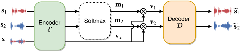
(a) Step 1: Learning the latent targets.

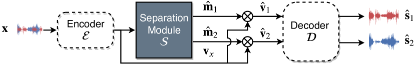
(b) Step 2: Training the separation module only.

Fig. 1: Training a separation network in two independent steps. For each step, the non-trainable parts are represented with a dashed line.

2.1 Step 1: Learning the Latent Targets

As a first step we train an encoder $\mathcal{E}$ in order to obtain a latent representation for the mixture $\textbf{v}_{\textbf{x}}=\mathcal{E}\left(\textbf{x}\right)$. We also provide the clean sources as inputs to this encoder to obtain $\textbf{v}_{1},\cdots,\textbf{v}_{N}$ and apply a softmax function (across the dimension of the sources) in order to obtain separation masks $\textbf{m}_{1},\cdots,\textbf{m}_{N}$ for each source. An element-wise multiplication of these masks with the latent representation of the mixture $\textbf{v}_{i}=\textbf{m}_{i}\odot\textbf{v}_{\textbf{x}},\enskip\forall i\in\{1,\cdots,N\}$, can be used as an estimate for each source. The decoder module $\mathcal{D}$ is then trained to transform these latent representations back to time-domain using $\widetilde{\textbf{s}}_{i}=\mathcal{D}\left(\textbf{v}_{\textbf{i}}\right),\enskip\forall i\in\{1,\cdots,N\}$. In order to train the encoder and the decoder we optimize the permutation invariant [21] SI-SDR [22] between the clean sources s and the estimated sources $\widetilde{\textbf{s}}$:

$$\begin{gathered}\mathcal{L}_{1}=-\text{SI-SDR}(\textbf{s}^{*},\widetilde{\textbf{s}})=-10\log_{10}\left(\|\alpha\textbf{s}^{*}\|^{2}/\|\alpha\textbf{s}^{*}-\widetilde{\textbf{s}}\|^{2}\right)\end{gathered}$$ (1)

where $\textbf{s}^{*}$ denotes the permutation of the sources that maximizes SI-SDR and the scalar $\alpha=\widetilde{\textbf{s}}^{\top}\textbf{s}^{*}/\|\textbf{s}\|^{2}$ ensures that the loss is scale invariant. A schematic representation of the aforementioned step for two sources is depicted in Fig. 1(a). The objective of this step is to find a latent representation transformation, which facilitates source separation through masking.

2.2 Step 2: Training the Separation Module

Once the weights of the encoder and decoder modules are fixed using the training recipe described in Step 1, we can train a separation module $\mathcal{S}$. Given the latent representation of an input mixture $\textbf{v}_{\textbf{x}}=\mathcal{E}\left(\textbf{x}\right)$, $\mathcal{S}$ is trained to produce an estimate of the latent representation $\hat{\textbf{v}}_{i}$ for each clean source $\textbf{v}_{i}$, i.e. $\hat{\textbf{v}}=\mathcal{S}\left(\textbf{v}_{\textbf{x}}\right)$. During inference, we can use the pre-trained decoder to transform the source estimates back into the time-domain $\hat{\textbf{s}}=\mathcal{D}\left(\mathcal{S}\left(\textbf{v}_{\textbf{x}}\right)\right)$. The block diagram describing the training of the separation module with a fixed encoder and decoder is shown in Fig. 1(b).

2.2.1 Training using SI-SDR on the Latent Separation Targets

In contrast to recent time-domain source-separation approaches [23, 7] which train all modules $\mathcal{E}$, $\mathcal{D}$, and $\mathcal{S}$ using a variant of the loss defined in Eq. 1, we propose to use the permutation invariant SI-SDR directly on the latent representation. For simplicity of notation we assume that each source has a vector latent representation $\textbf{v}_{i}\in\mathbb{R}^{K}$ in a high dimensional space. The loss for training the separation module could then be: $\mathcal{L}_{2}=-\text{SI-SDR}(\textbf{v}^{*},\hat{\textbf{v}})$. The exact same training procedure could be followed, but now we can use as targets the optimal separation targets on the latent space as opposed to the time domain signals. The premise is that if the separation module is trained on producing latent representations $\hat{\textbf{v}}\approx\textbf{v}$ which are close to the ideal ones (assuming ideal permutation order) then the estimates of the sources after the decoding layer would also approximate the clean sources in time-domain $\hat{\textbf{s}}=\mathcal{D}\left(\mathcal{S}\left(\textbf{v}_{\textbf{x}}\right)\right)\approx\mathcal{D}\left(\textbf{v}\right)=\widetilde{\textbf{s}}\approx\textbf{s}$. The latter might not hold for any arbitrary embedding process, but in the next section we prove that SI-SDR in the latent representations lower-bounds the SI-SDR in the time-domain.

2.2.2 Relation to maximization of SI-SDR on Time-Domain

We restrict ourselves to a decoder that consists of a 1-D transposed convolutional layer which is the same as the decoder selection in most of the current end-to-end source separation approaches [23, 7, 17, 16]. For this part we focus on the $i$th target latent representation $\textbf{v}_{i}\in\mathbb{R}^{K}$ that corresponds to a source time-domain signal $\textbf{s}_{i}\in\mathbb{R}^{T}$. Because the encoder-decoder modules are trained as described in Section 2.1, the separation target produced by the auto-encoder $\widetilde{\textbf{s}}_{i}$ would be close to the clean source $\textbf{s}_{i}$, namely:

$$\mathcal{D}\left(\textbf{v}_{\textbf{i}}\right)=\widetilde{\textbf{s}}_{i}\approx\textbf{s}_{i}$$ (2)

The separation network produces an estimated latent vector $\hat{\textbf{v}}_{i}$ that corresponds to an estimated time-domain signal $\hat{\textbf{s}}_{i}=\mathcal{D}\left(\hat{\textbf{v}}_{i}\right)$. Because the decoder is just a convolutional layer we can express it as a linear projection $\mathcal{D}:\mathbb{R}^{K}\rightarrow\mathbb{R}^{T}$ using the matrix $\textbf{P}\in\mathbb{R}^{T\times K}$:

$$\hat{\textbf{s}}_{i}=\textbf{P}\hat{\textbf{v}}_{i},\enskip\widetilde{\textbf{s}}_{i}=\textbf{P}\textbf{v}_{i},\enskip\forall i\in\{1,\cdots,N\}$$ (3)

Assuming the Moore-Penrose pseudo-inverse of P is well defined, we express the inverse mapping from time to the latent-space as:

$$\hat{\textbf{v}}_{i}=\textbf{P}^{\dagger}\hat{\textbf{s}}_{i},\enskip\textbf{v}_{i}=\textbf{P}^{\dagger}\widetilde{\textbf{s}}_{i},\enskip\forall i\in\{1,\cdots,N\}$$ (4)

Proposition 1.

Let $\textbf{y},\hat{\textbf{y}}\in\mathbb{R}^{d}$ and their corresponding projections through $\textbf{A}\in\mathbb{R}^{n\times d}$ to $\mathbb{R}^{n}$ defined as Ay and $\textbf{A}\hat{\textbf{y}}$, respectively. If $\|\textbf{y}\|=\|\hat{\textbf{y}}\|=1$ then the absolute value of their inner product on the projection space $\mathbb{R}^{n}$ is bounded above from the absolute value of their inner product in $\mathbb{R}^{d}$, namely: $\left(\hat{\textbf{y}}^{\top}\textbf{A}^{\top}\textbf{A}\textbf{y}\right)^{2}\leq g\left(\textbf{A}\right)+\left(\hat{\textbf{y}}^{\top}\textbf{y}\right)^{2}$, where $g\left(\textbf{A}\right)\geq 0$ and depends only on the values of A.

Proof.

The inner product in the projection space can be rewritten as:

$$\begin{gathered}\left(\hat{\textbf{y}}^{\top}\textbf{A}^{\top}\textbf{A}\textbf{y}\right)^{2}=\left[\hat{\textbf{y}}^{\top}\left(\textbf{A}^{\top}\textbf{A}-\textbf{I}\right)\textbf{y}+\hat{\textbf{y}}^{\top}\textbf{y}\right]^{2}=\\ \left[\hat{\textbf{y}}^{\top}\left(\textbf{A}^{\top}\textbf{A}-\textbf{I}\right)\textbf{y}\right]^{2}+2\left[\hat{\textbf{y}}^{\top}\left(\textbf{A}^{\top}\textbf{A}-\textbf{I}\right)\textbf{y}\hat{\textbf{y}}^{\top}\textbf{y}\right]+\left(\hat{\textbf{y}}^{\top}\textbf{y}\right)^{2}\end{gathered}$$ (5)

Moreover, we can bound the first term of Eq. 5 by applying Cauchy-Schwarz inequality to the inner products and using the fact that $\|\textbf{y}\|=\|\hat{\textbf{y}}\|=1$ as shown next:

$$\begin{gathered}\left[\hat{\textbf{y}}^{\top}\left(\textbf{A}^{\top}\textbf{A}-\textbf{I}\right)\textbf{y}\right]\leq\|\hat{\textbf{y}}\|\cdot\|\textbf{A}^{\top}\textbf{A}-\textbf{I}\|\cdot\|\textbf{y}\|=\|\textbf{A}^{\top}\textbf{A}-\textbf{I}\|\end{gathered}$$ (6)

Similarly, we use Cauchy-Schwarz inequality and inequality 6 in order to bound the second term of Eq. 5 as well:

$$\begin{gathered}\left[\hat{\textbf{y}}^{\top}\left(\textbf{A}^{\top}\textbf{A}-\textbf{I}\right)\textbf{y}\hat{\textbf{y}}^{\top}\textbf{y}\right]\leq\|\textbf{A}^{\top}\textbf{A}-\textbf{I}\|\end{gathered}$$ (7)

Then by applying inequalities 6 and 7 to Eq. 5 we get:

$$\begin{split}\left(\hat{\textbf{y}}^{\top}\textbf{A}^{\top}\textbf{A}\textbf{y}\right)^{2}&\leq\|\textbf{A}^{\top}\textbf{A}-\textbf{I}\|^{2}+2\cdot\|\textbf{A}^{\top}\textbf{A}-\textbf{I}\|+\left(\hat{\textbf{y}}^{\top}\textbf{y}\right)^{2}\end{split}$$ (8)

where always $g\left(\textbf{A}\right)=\|\textbf{A}^{\top}\textbf{A}-\textbf{I}\|^{2}+2\cdot\|\textbf{A}^{\top}\textbf{A}-\textbf{I}\|\geq 0$. Finally, we conclude that $\left(\hat{\textbf{y}}^{\top}\textbf{A}^{\top}\textbf{A}\textbf{y}\right)^{2}\leq g\left(\textbf{A}\right)+\left(\hat{\textbf{y}}^{\top}\textbf{y}\right)^{2}$. ∎

Proposition 2.

Let $\textbf{y},\hat{\textbf{y}}\in\mathbb{R}^{d}$, with unit norms, then maximizing $\text{SI-SDR}(\textbf{y},\hat{\textbf{y}})$ w.r.t. $\hat{\textbf{y}}$ is equivalent to maximizing $\left(\hat{\textbf{y}}^{\top}\textbf{y}\right)^{2}$ w.r.t. $\hat{\textbf{y}}$.

Proof.

By assuming that there is an optimal solution $\hat{\textbf{y}}^{\star}$:

$$\begin{split}\hat{\textbf{y}}^{\star}&=\underset{\hat{\textbf{y}}}{\operatorname{\arg\max}}\enskip\text{SI-SDR}(\textbf{y},\hat{\textbf{y}})\xlongequal{Eq.\ref{eq:step1SISDR}}\underset{\hat{\textbf{y}}}{\operatorname{\arg\max}}\enskip\frac{\|\alpha\textbf{y}\|^{2}}{\|\alpha\textbf{y}-\hat{\textbf{y}}\|^{2}}=\\ &=\underset{\hat{\textbf{y}}}{\operatorname{\arg\max}}\enskip\frac{\|\alpha\textbf{y}\|^{2}}{\|\alpha\textbf{y}\|^{2}+\|\hat{\textbf{y}}\|^{2}-2\alpha\hat{\textbf{y}}^{\top}\textbf{y}}=\\ &=\underset{\hat{\textbf{y}}}{\operatorname{\arg\max}}\left[1+\frac{\|\hat{\textbf{y}}\|^{2}}{\|\textbf{y}\|^{2}\alpha^{2}}-2\frac{\hat{\textbf{y}}^{\top}\textbf{y}}{\alpha\|\textbf{y}\|^{2}}\right]^{-1}\xlongequal{\alpha=\nicefrac{{\hat{\textbf{y}}^{\top}\textbf{y}}}{{\|\textbf{y}\|^{2}}}}\\ &=\underset{\hat{\textbf{y}}}{\operatorname{\arg\max}}\frac{\left(\hat{\textbf{y}}^{\top}\textbf{y}\right)^{2}}{\|\textbf{y}\|^{2}\|\hat{\textbf{y}}\|^{2}}\xlongequal{\|\textbf{y}\|=\|\hat{\textbf{y}}\|=1}\underset{\hat{\textbf{y}}}{\operatorname{\arg\max}}\left(\hat{\textbf{y}}^{\top}\textbf{y}\right)^{2}\end{split}$$ (9)

Which means that the two optimization goals are equivalent. ∎

Now we focus on the relationship of the maximization of SI-SDR for the $i$th source when it is performed directly on the latent space $\text{SI-SDR}(\textbf{v}_{i},\hat{\textbf{v}}_{i})$ and when it is performed on the time-domain using the clean source as a target $\text{SI-SDR}(\textbf{s}_{i},\hat{\textbf{s}}_{i})\approx\text{SI-SDR}(\widetilde{\textbf{s}}_{i},\hat{\textbf{s}}_{i})$. Again because all the SI-SDR measures are scale-invariant, we can assume that the separation targets and the estimates vectors have unit norms on both the time-domain and the latent space, namely $\|\hat{\textbf{v}}_{i}\|=\|\textbf{v}_{i}\|=\|\hat{\textbf{s}}_{i}\|=\|\widetilde{\textbf{s}}_{i}\|=1$. By using Proposition 1 we get:

$$\left(\hat{\textbf{v}}_{i}^{\top}\textbf{v}_{i}\right)^{2}=\left[\hat{\textbf{s}}_{i}^{\top}\left(\textbf{P}^{\dagger}\right)^{\top}\textbf{P}^{\dagger}\widetilde{\textbf{s}}_{i}\right]^{2}\leq g\left(\textbf{P}^{\dagger}\right)+\left(\hat{\textbf{s}}_{i}^{\top}\widetilde{\textbf{s}}_{i}\right)^{2}$$ (10)

Thus, by using the auto-encoder property (Eq. 2) and Proposition 2 we conclude that $\text{SI-SDR}(\textbf{v}_{i},\hat{\textbf{v}}_{i})$ on the latent space lower bounds the corresponding value $\text{SI-SDR}(\textbf{s}_{i},\hat{\textbf{s}}_{i})$ on the time-domain. The same proof holds for any encoder $\mathcal{E}$ and for other targets on the latent space such as the masks $\textbf{m}_{i}\in[0,1]^{K}$. Empirically, we indeed notice that the maximization of $\text{SI-SDR}(\textbf{v}_{i},\hat{\textbf{v}}_{i})$ on the latent space leads to the maximization of $\text{SI-SDR}(\textbf{s}_{i},\hat{\textbf{s}}_{i})$ on the time-domain.

3 Experimental Framework

To experimentally verify our approach we perform a set of source separation experiments as described in the following sections.

3.1 Audio Data

We use two audio data collections. For speech sources we use $14,823$ speech utterances from Wall street journal (WSJ0) corpus [24]. Training, validation and test speaker mixtures are generated by randomly selecting various speakers from the sets si_tr_s, si_dt_05 and si_et_05, respectively.

For non-speech sounds we use the $2,000$ $5$secs audio clips which are equally balanced between $50$ classes from the environmental sound classification (ESC50) data collection [25]. ESC50 spans various sound categories such as: non-speech human sounds, animal sounds, natural soundscapes, interior sounds and urban noises. We split the data to train, validation and test sets with a ratio of $8:1:1$, respectively. For each set, the same prior is used across classes (e.g., each class has the same number of clips). Also, the sets do not share clips which originate from the same initial source file.

3.2 Sound Source Separation Tasks

In order to develop a system capable of performing universal sound source separation [17], we evaluate our two-step approach under three distinct sound separation tasks. For all separation tasks, each input mixture consists of two sources which are always mixed using $4$secs of their total duration. All audio clips are downsampled to $8$kHz for efficient processing. We discuss the audio collection(s) that we utilize and the mixture generation process in the sections below.

3.2.1 Speech Separation

We only use audio clips containing human speech from WSJ0. In accordance to other studies performing experiments on single-channel speech source separation [7, 26, 27, 15, 8], we use the publicly available WSJ0-2mix dataset [5]. In total there are $20,000$, $5,000$ and $3,000$ mixtures for training, validation and testing, correspondingly.

3.2.2 Non-Speech Separation

We use audio clips only from ESC50. In this case, the total number of the available clean sources sounds is small, and thus, we propose an augmented mixture generation process which enables the generation of much more diverse mixtures. In order to generate each mixture, we randomly select a $4$sec segment from two audio files from two distinct audio classes. We mix these two segments with a random signal to noise ratio (SNR)s between $-2.5$ and $2.5$dB. For each epoch, $20,000$ training mixtures are generated which generally are not the same with the ones generated for other epochs. For validation and test sets we fix their random seeds in order to always evaluate on the same $5,000$ and $3,000$ generated mixtures, respectively.

3.2.3 Mixed Separation

All four possible mixture combinations between speech and non-speech audio are considered by using both WSJ0 and ESC50 sources. Building upon the data augmentation training idea, we also add a random variable which controls the data collection (ESC50 or WSJ0) from which a source waveform is going to be chosen. Specifically, we set an equal probability of choosing a source file from the two collections (ESC50 and WSJ0). For WSJ0 each speaker is considered a distinct sound class, thus, no mixture consists utterances from the same speaker. After the two source waveforms are chosen, we follow the mixture generation process described in Section 3.2.2.

3.3 Selected Network Architectures

Based on recent state-of-the-art approaches on both speech and universal sound source separation with learnable encoder and decoder modules, we consider configurations for the encoder-decoder parts as well as the separation module which are based on a similar time-dilated convolutional network (TDCN) architecture. In particular, we consider our implementations of ConvTasNet [7] that we refer simply as TDCN and its improved version proposed in [17] that we refer as residual-TDCN (RTDCN).

3.3.1 Encoder-Decoder Architecture

The encoder $\mathcal{E}$ consists of one $1$D convolutional layer and a ReLU activation on top in order to ensure a non-negative latent representation of each audio input. Following the assumptions stated in Section 2.2.2, we use a $1$D transposed convolutional layer for the decoder $\mathcal{D}$. Both encoder and decoder have the same number of channels (or number of bases) and their $1$D kernels have a length corresponding to $2.625$ms ($21$ samples) and a hop-size equivalent to $1.25$ms ($10$ samples). For each task we select a different number of channels for the encoder and the decoder modules ($32$, $128$ and $256$ for speech only, mixed and non-speech only separation tasks, respectively).

3.3.2 Separation Modules Architectures

Our implementation of TDCN consists of the same architecture and parameter configuration for the separation module as described in [7] with an additional batch normalization layer before the final mask estimation which improved its performance over the original version on all separation tasks. Inspired by the original RTDCN separation module [17], we keep the same parameter configuration as TDCN and we additionally use a feature-wise normalization between layers instead of global normalization. We also add long-term residual connections from previous layers. Moreover, before summing the residual connections, we concatenate them, normalize them and feed them through a dense layer as the latter yields some further improvement in separation performance. (Code is available online.)

3.4 Training and Evaluation Details

In order to show the effectiveness of our proposed two-step approach, we use the same network architecture when we perform end-to-end time-domain source separation and use as a loss the negative SI-SDR between the estimated signals on the time-domain and the clean waveforms $-\text{SI-SDR}(\hat{\textbf{s}},\textbf{s}^{*})$. Instead in our two-step approach, we train the encoder-decoder parts separately as described in Section 2.1. In the second step, we use the pre-trained encoders for each task and train the separation module using as loss the negative SI-SDR on the latent space targets $-\text{SI-SDR}(\textbf{v}^{*},\hat{\textbf{v}})$ or their corresponding masks $-\text{SI-SDR}(\textbf{m}^{*},\hat{\textbf{m}})$ (see Section 2.2). We train all models using the Adam optimizer [28], the batch size is equal to $4$, the initial learning rate is set to $0.001$ and we decrease it by a factor of $10$ at the $100$th epoch. We train TDCN and RTDCN separation networks for $100$ epochs and $120$ epochs, respectively. The encoder-decoder parts for each task are trained independently for $200$ epochs ($100$ times faster than training the separation network). We evaluate the separation performance for all models using SI-SDR improvement (SI-SDRi) on time domain which is the difference of SI-SDR of the estimated signal and the input mixture signal [7, 17]. As the STFT oracle mask we choose the ideal ratio mask (IRM) using a Hanning window with $64$ms length and $16$ms hop-size [7].

4 Results & Discussion

4.1 Comparison with Time-Domain Separation

In Table 1, the mean separation performance of best models is reported for each task. We notice that the proposed two-step approach and training on the latent space leads to a consistent improvement over the end-to-end approach where we train the same architecture using the time-domain SI-SDR loss. This observation holds when different separation modules are used and when we test them under different separation tasks. The non-speech separation task seems the hardest one since the models have access to only a limited number of training mixtures which further underlines the importance of our proposed data-augmentation technique as described in Section 3.2.2. Our two-step approach yields an absolute SI-SDR improvement over the end-to-end baseline of up to $0.7$dB, $0.5$dB and $0.7$dB for speech, non-speech and mixed separation tasks, respectively. Notably, this performance improvement is achieved using the exact same architecture but instead of training it end-to-end using a time-domain loss, we pre-train the auto-encoder part and use a loss on the latent representations of the sources.

Separation					Target	Sound Separation Task
Module	Domain	Speech	Non-speech	Mixed
TDCN	Time	15.4	7.7	11.7
	Latent	16.1	8.2	12.4
RTDCN	Time	15.6	8.3	12.0
	Latent	16.2	8.4	12.6
Oracle	STFT	13.0	14.8	14.5
Masks	Latent	34.1	39.2	39.5

Table 1: Mean SI-SDRi (dB) of best performing models.

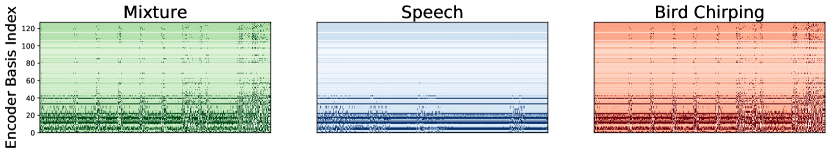
(a) Two-step training approach.

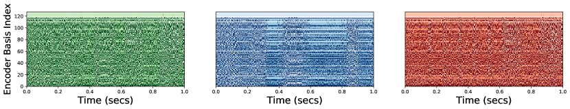
(b) Joint end-to-end training using time-domain SI-SDR loss.

Fig. 2: Latent representations of a $1$sec mixture and its constituent sources when training the same encoder architecture: a) individually using the proposed two-step approach (top) b) jointly with the TDCN separation module using SI-SDR loss on time-domain (bottom). We sort the basis indexes w.r.t. their energy and we raise the value of each cell to $0.1$ for better visualization.

4.2 Separation Targets in the Latent Space

In Table 1, we see that the oracle mask obtained from the two-step approach gives a much higher upper bound of separation performance, for all tasks, compared to ideal masks on the STFT domain. This is in line with the prior work that proposed to decompose signals using learned transforms [7, 16]. In Fig. 2 we can qualitatively compare the latent representations obtained from the same encoder when trained with our proposed two-step approach and with the baseline joint training of all modules. When the encoder and decoder are trained individually, a fewer number of bases are used to encode the input which leads to a sparser representation ($\ell_{1}$ norm is roughly $10\times$ smaller compared to the joint training approach). Finally, the latent representations obtained from our proposed approach exhibit a spectrogram-like structure in a way that Speech is encoded using less bases than high frequency sounds like Bird Chirping.

5 Conclusion

We show how by pre-learning an optimal latent space can result in better source separation performance compared to a time-domain end-to-end training approach. Our experiments show that the proposed two-step approach yields a consistent performance improvement under multiple sound separation tasks. Additionally, the obtained sound latent representations remain sparse and structured while they also enjoy a much higher upper bound of separation performance compared to STFT-domain masks. Although this approach was demonstrated on TDCN architectures, it can be easily adapted for use with any other mask-based system.

References

- [1] Adel Belouchrani and Moeness G Amin, “Blind source separation based on time-frequency signal representations,” IEEE Transactions on Signal Processing, vol. 46, no. 11, pp. 2888–2897, 1998.
- [2] Seungjin Choi, Andrzej Cichocki, Hyung-Min Park, and Soo-Young Lee, “Blind source separation and independent component analysis: A review,” Neural Information Processing-Letters and Reviews, vol. 6, no. 1, pp. 1–57, 2005.
- [3] Jonathan Le Roux, John R Hershey, and Felix Weninger, “Deep nmf for speech separation,” in Proc. ICASSP, 2015, pp. 66–70.
- [4] Po-Sen Huang, Minje Kim, Mark Hasegawa-Johnson, and Paris Smaragdis, “Deep learning for monaural speech separation,” in Proc. ICASSP, 2014, pp. 1562–1566.
- [5] John R Hershey, Zhuo Chen, Jonathan Le Roux, and Shinji Watanabe, “Deep clustering: Discriminative embeddings for segmentation and separation,” in Proc. ICASSP, 2016, pp. 31–35.
- [6] Andreas Jansson, Eric J. Humphrey, Nicola Montecchio, Rachel M. Bittner, Aparna Kumar, and Tillman Weyde, “Singing voice separation with deep u-net convolutional networks,” in Proc. ISMIR, 2017, pp. 323–332.
- [7] Yi Luo and Nima Mesgarani, “Conv-tasnet: Surpassing ideal time–frequency magnitude masking for speech separation,” IEEE/ACM Transactions on Audio, Speech, and Language Processing, vol. 27, no. 8, pp. 1256–1266, 2019.
- [8] Zhong-Qiu Wang, Ke Tan, and DeLiang Wang, “Deep learning based phase reconstruction for speaker separation: A trigonometric perspective,” in Proc. ICASSP, 2019, pp. 71–75.
- [9] Efthymios Tzinis, Shrikant Venkataramani, and Paris Smaragdis, “Unsupervised deep clustering for source separation: Direct learning from mixtures using spatial information,” in Proc. ICASSP, 2019, pp. 81–85.
- [10] Prem Seetharaman, Gordon Wichern, Jonathan Le Roux, and Bryan Pardo, “Bootstrapping single-channel source separation via unsupervised spatial clustering on stereo mixtures,” in Proc. ICASSP, 2019, pp. 356–360.
- [11] Lukas Drude, Daniel Hasenklever, and Reinhold Haeb-Umbach, “Unsupervised training of a deep clustering model for multichannel blind source separation,” in Proc. ICASSP, 2019, pp. 695–699.
- [12] Po-Sen Huang, Minje Kim, Mark Hasegawa-Johnson, and Paris Smaragdis, “Joint optimization of masks and deep recurrent neural networks for monaural source separation,” IEEE/ACM Transactions on Audio, Speech, and Language Processing, vol. 23, no. 12, pp. 2136–2147, 2015.
- [13] Jahn Heymann, Lukas Drude, and Reinhold Haeb-Umbach, “Neural network based spectral mask estimation for acoustic beamforming,” in Proc. ICASSP, 2016, pp. 196–200.
- [14] Yusuf Isik, Jonathan Le Roux, Zhuo Chen, Shinji Watanabe, and John R Hershey, “Single-channel multi-speaker separation using deep clustering,” in Proc. Interspeech, 2016, pp. 545–549.
- [15] Gordon Wichern and Jonathan Le Roux, “Phase reconstruction with learned time-frequency representations for single-channel speech separation,” in Proc. IWAENC, 2018, pp. 396–400.
- [16] Shrikant Venkataramani, Jonah Casebeer, and Paris Smaragdis, “End-to-end source separation with adaptive front-ends,” in Proc. Asilomar Conference on Signals, Systems, and Computers, 2018, pp. 684–688.
- [17] Ilya Kavalerov, Scott Wisdom, Hakan Erdogan, Brian Patton, Kevin Wilson, Jonathan Le Roux, and John R Hershey, “Universal sound separation,” Proc. WASPAA, 2019.
- [18] Emad M Grais, Gerard Roma, Andrew JR Simpson, Mark D Plumbley, Emad M Grais, Gerard Roma, Andrew JR Simpson, and Mark D Plumbley, “Two-stage single-channel audio source separation using deep neural networks,” IEEE/ACM Transactions on Audio, Speech and Language Processing (TASLP), vol. 25, no. 9, pp. 1773–1783, 2017.
- [19] Yuzhou Liu and DeLiang Wang, “Divide and conquer: A deep casa approach to talker-independent monaural speaker separation,” arXiv preprint arXiv:1904.11148, 2019.
- [20] Jacob Devlin, Ming-Wei Chang, Kenton Lee, and Kristina Toutanova, “Bert: Pre-training of deep bidirectional transformers for language understanding,” in Proceedings of the 2019 Conference of the North American Chapter of the Association for Computational Linguistics: Human Language Technologies, Volume 1 (Long and Short Papers), 2019, pp. 4171–4186.
- [21] Dong Yu, Morten Kolbæk, Zheng-Hua Tan, and Jesper Jensen, “Permutation invariant training of deep models for speaker-independent multi-talker speech separation,” in Proc. ICASSP, 2017, pp. 241–245.
- [22] Jonathan Le Roux, Scott Wisdom, Hakan Erdogan, and John R Hershey, “Sdr–half-baked or well done?,” in Proc. ICASSP, 2019, pp. 626–630.
- [23] Yi Luo and Nima Mesgarani, “Tasnet: time-domain audio separation network for real-time, single-channel speech separation,” in Proc. ICASSP, 2018, pp. 696–700.
- [24] Douglas B. Paul and Janet M. Baker, “The design for the wall street journal-based CSR corpus,” in Speech and Natural Language: Proceedings of a Workshop Held at Harriman, New York, February 23-26, 1992, 1992.
- [25] Karol J Piczak, “Esc: Dataset for environmental sound classification,” in Proc. ACM International Conference on Multimedia, 2015, pp. 1015–1018.
- [26] Ziqiang Shi, Huibin Lin, Liu Liu, Rujie Liu, Shoji Hayakawa, and Jiqing Han, “Furcax: End-to-end monaural speech separation based on deep gated (de) convolutional neural networks with adversarial example training,” in Proc. ICASSP, 2019, pp. 6985–6989.
- [27] Jonathan Le Roux, Gordon Wichern, Shinji Watanabe, Andy Sarroff, and John R Hershey, “Phasebook and friends: Leveraging discrete representations for source separation,” IEEE Journal of Selected Topics in Signal Processing, vol. 13, no. 2, pp. 370–382, 2019.
- [28] Diederik P Kingma and Jimmy Ba, “Adam: A method for stochastic optimization,” arXiv preprint arXiv:1412.6980, 2014.