$\bm{J}$ Regularization Improves Imbalanced Multiclass Segmentation

Abstract

We propose a new loss formulation to further advance the multiclass segmentation of cluttered cells under weakly supervised conditions. We improve the separation of touching and immediate cells, obtaining sharp segmentation boundaries with high adequacy, when we add Youden’s $J$ statistic regularization term to the cross entropy loss. This regularization intrinsically supports class imbalance thus eliminating the necessity of explicitly using weights to balance training. Simulations demonstrate this capability and show how the regularization leads to better results by helping advancing the optimization when cross entropy stalls. We build upon our previous work on multiclass segmentation by adding yet another training class representing gaps between adjacent cells. This addition helps the classifier identify narrow gaps as background and no longer as touching regions. We present results of our methods for 2D and 3D images, from bright field to confocal stacks containing different types of cells, and we show that they accurately segment individual cells after training with a limited number of annotated images, some of which are poorly annotated.

Index Terms—  Loss modeling, deep learning, instance segmentation, multiclass segmentation, cell segmentation, data imbalance

1 Introduction

The long-term goal of our work has been the automatic segmentation of cells found in different modalities of microscope images so that it can ultimately help in the quantification of biological studies (see e.g. [1, 2, 3, 4]). The task remains a challenge particularly when cells are densely packed in clusters exhibiting a range of signals and when training with a small number of weak annotations (see Fig.1). Separation of cluttered cells is especially difficult when shared edges have low contrast and are similar to cell interiors. Weak annotations, when incomplete and inaccurate, can harm the learning process as the optimizer might be confused when deciding if annotated and non-annotated regions with same patterns must be segmented or not. Our proposed solutions aim to resolve these problems with advances in loss formulation, class imbalance handling, multiclass classification, and data augmentation.

We propose a new deep learning multiclass segmentation method which classifies pixels into four distinct classes – background, cell, touching, and gap – by minimizing a loss function that penalizes both cross entropy and Youden’s $J$ statistic. Pixels and voxels classified as touching and gap become either cell or background in a post-processing step, producing a final segmentation containing a single mask for each individual cell in the image.

We build upon our recent work [1, 2] to further improve multiclass cell segmentation. The introduction of a fourth class, named gap, and of a new loss lead to better segmentations where small regions separating nearby cells are now correctly classified as background regions. Slim cell protrusions are also correctly classified thanks to the balancing offered by our proposed loss.

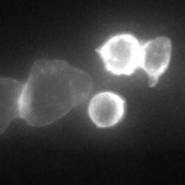
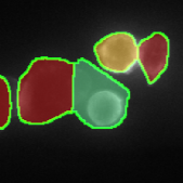
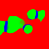
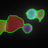
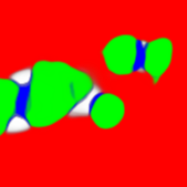
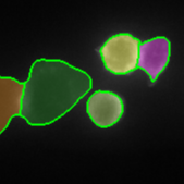
Image	Annotation	$\bm{J3}$ Probability	$\bm{J3}$ Segmentation	$\bm{J4}$ Probability	$\bm{J4}$ Segmentation

Fig. 1: A poorly annotated test image is segmented with our $J$ regularized loss, $\mathcal{L}_{JC}$, using three, $J3$, and four, $J4$, semantic classes. We obtain a correct segmentation when training with an added fourth class representing gaps and cavities – predicted white patches shown on $J4$ Probability. The result is superior to the annotation, which, unintentionally, missed tracing the right contour on the round central cell above. The training of our models has been consistently robust despite the presence of weakly annotated images, which are present in the total training data. Background (red), cell (green), touching (blue), and gap (white) are the four classes predicted by our models.

 

Previous work. Recent modeling of new loss functions for segmentation [1, 5, 6, 7] incorporates a differentiable surrogate over a known performance measurement. Unfortunately these are not sufficient to cope with high data imbalance typical when segmenting biomedical images. In [8] the authors review regional losses and propose a contour based loss as an alternative to combat imbalance. The work of Brosch et al. [9] bears similarities to ours as they model their loss as a linear combination of sensitivity and specificity measures. But they use mean square errors instead and recommend heavily weighting specificity, 95%, in detriment to sensitivity, 5%, which we believe goes against the importance of equally balancing both measures. Sudre et al. [10] proposed using the generalized dice overlap introduced in [11] as a loss function to avert imbalance in segmentation. Imbalance is achieved by explicitly weighting classes as in [12] but now inversely proportional to the square number of pixels. From our experience, this works to isolate cell clusters but it is not enough to isolate cells in a cluster.

Pixel weights have been adopted as a strategy to balance data [12, 9] including shape aware weights [2]. While advantageous they are not sufficient to fully separate packed cells or resolve fine details. Equibatches [7] is yet another balancing strategy for segmentation. It forces training examples from all classes to be present during every training iteration. Multiclass deep learning training for cell segmentation is adopted in [2] for 2D images and in [13] for 3D confocal stacks.

2 Method

Notation. The goal of panoptic segmentation is to assign to each pixel or voxel $p\in\Omega$ of a single channel image $x\colon\Omega\subset\mbox{$\mathbbm{R}^{d}$}\to\mbox{$\mathbbm{R}^{+}$}$ a semantic label, and an instance label when $p$ belongs to a countable category [14]. For learning a segmentation we are given a training set $S=\{(x_{i},g_{i})\}$ where for every image $x_{i}$ we know its ground truth segmentation $g_{i}$. In general, we have $g\colon\Omega\to\{0,\ldots,m\}$, a mapping where $g(p)=0$ for $p$ in the background and $0<g(p)\leqslant m$ is a unique label for each object in the image. Our task is cast as a semantic segmentation problem by modifying the approach proposed in [1] to transform the instance annotation $g$ into a semantic ground truth $h$, generalizing to high dimensions by using a $(2k+1)^{d}$ neighborhood $\eta_{k}(p),k\geqslant 1$. Let $y\colon\Omega\to\mbox{$\mathbbm{R}^{C+1}$}$ be the one hot representation for the $C$-classes in the semantic mapping $h\colon\Omega\to\{0,\ldots,C\}$, and $n_{l}=\sum_{p\in\Omega}y_{l}(p)$ the number of elements of class $l$. We call $\varrho_{e}\colon\Omega\to\mbox{$\mathbbm{R}^{+}$}$ the bottom hat transform over $g$ using structuring element $e$, a hyper-sphere whose size is data dependent. The output of our trained network is a probability map $z$ such that $z(p)\approx y(p),\forall p$. A post-processing similar to the one proposed in [1] is then applied to build a panoptic segmentation $\hat{g}$ from $z$.

Gap class. We have previously shown that using three semantic classes, namely image background, cell interior, and touching region, increases the network discriminative power when segmenting cluttered cells [2, 1]. However, misclassified background regions persisted in some cases, see Fig.1. We speculate this is due to losing background information when merging nearby cells in the U-Net contracting path, information which is not fully recovered in the up–sampling path. By introducing a new training class representing the gap between nearby cells, the network can now classify the regions separating nearby cells as background. We name this new class, not surprisingly, gap – white pixels shown in $J4$, Fig.1. These regions are obtained using the bottom hat transform. Given an instance annotation $g$, a semantic ground truth $h$ of our four classes is defined as

$$h(p)=\left\{\begin{aligned} 0&\;\;\text{if }g(p)=0\text{ and }\varrho_{e}(p)=0-{\scriptsize\text{\em background}}\\ 3&\;\;\text{if }g(p)=0\text{ and }\varrho_{e}(p)>0-{\scriptsize\text{\em gap}}\\ 2&\;\;\text{if }g(p^{\prime})\neq g(p)\text{ and}\ g(p^{\prime})\neq 0,\forall{p^{\prime}\in\eta_{k}(p)}-{\scriptsize\text{\em touching}}\\ 1&\;\;\text{otherwise}-{\scriptsize\text{\em cell}}\\ \end{aligned}\right.$$

If $p$ is in the background and lies in the bottom hat transform, then $p$ is a gap pixel/voxel, $h(p)=3$. We use $k=2$ in our experiments.

2.1 $\bm{J}$ regularization

The J statistic was formulated by statistician William J. Youden to improve rating the performance of diagnostic tests of diseases [15]. A high index $J$ for a test would imply that this test could predict with high probability if an individual was diseased or not. An ideal test would be able to eliminate false negatives (sick, at risk individuals falsely reported as healthy) and false positives (healthy individuals falsely reported as sick) thus always reporting with certainty diseased (true positive) and healthy (true negative) individuals. Youden modeled $J$ as the average success of a test on reporting the proportions of diseased and healthy individuals. The effectiviness of this index in binary classification is due to the equal importance it gives to correctly classifying the subjects belonging and not belonging to a class, giving equal weight to true positive (sensitivity) and true negative (specificity) rates. $J$ is thus a suitable measure for predicting segmentation with our imbalanced classes: we typically have $n_{0}\gg n_{1}\gg n_{2}\approx n_{3}$, i.e. touching and gap classes are comprised of a few pixels/voxels when compared to background and cell classes. We can write $J=sensitivity+specificity-1=TPR+TNR-1$. We thus have $J\in[-1,1]$, and we aim to penalize negative correlations [16] and obtain a high $J$ after training.

We borrow ideas from [17] to compare $J$ to other popular measures used in loss surrogates [5, 6, 7]. Note that the most common surrogate for Accuracy is the Cross Entropy loss [18]. Classifier C1 is a random prediction where each class has the same imbalance ratio $\pi$ as in the ground truth. C3 is a random prediction with uniform distribution for all classes, $\pi=0.5$. As can be seen in Fig.2 the performance of $J$ under different imbalance ratios $\pi\in[0.01,0.50]$ is similar to the Matthews Correlation Coefficient, MCC [19], which is well-known to perform well under highly imbalanced data [17]. This is not the case for the Jaccard index , F1 (Dice) score, Tversky index, and Accuracy, as they all report different values for different imbalance ratio $\pi$. $J$ should thus be favored when training with imbalanced classes.

\begin{overpic}[height=130.08731pt]{C1.pdf} \put(54.0,2.0){{ $\pi$}} \put(72.0,60.0){{ C1}} \end{overpic}

\begin{overpic}[height=130.08731pt]{C3.pdf} \put(10.0,72.0){{ C3}} \put(105.0,35.0){{\includegraphics[height=35.45584pt]{legend.pdf}}} \put(110.0,72.5){{\scriptsize$J$}} \put(110.0,65.5){{\scriptsize MCC}} \put(110.0,57.5){{\scriptsize Jaccard}} \put(110.0,49.0){{\scriptsize F1}} \put(110.0,41.0){{\scriptsize Tversky}} \put(110.0,34.0){{\scriptsize Accuracy}} \put(49.0,2.0){{ $\pi$}} \end{overpic}

Fig. 2: Performance of classifiers C1 and C3 [17] measured by Youden’s $J$, Matthews Correlation Coefficient (MCC), Jaccard, F1 (Dice), Tversky, and Accuracy scores for different imbalance ratios $\pi$. Youden and MCC are the only ones almost completely invariant to all imbalance ratios.

 

To compare the correlation between $J$ and Matthews Correlation Coefficient, we used the settings for classifier C3 from [17]. We then measured the linear correlation between MCC and $J$ for imbalance ratios $\pi=0.01,0.25,0.50$ by using Pearson’s Correlation Coefficient. Fig.3 shows an almost perfect linear correlation for all ratios. This supports our claim that Youden’s $J$ index is a robust measure for imbalanced binary classification problems.

\begin{overpic}[grid=false,height=86.72267pt]{mvm1.pdf} \put(40.0,101.0){{\scriptsize$\pi=0.50$}} \put(65.0,12.0){{\scriptsize MCC}} \put(11.0,85.0){{\scriptsize$J$}} \end{overpic}

\begin{overpic}[grid=false,height=86.72267pt]{mvm3.pdf} \put(40.0,101.0){{\scriptsize$\pi=0.25$}} \put(65.0,12.0){{\scriptsize MCC}} \put(9.0,85.0){{\scriptsize$J$}} \end{overpic}

\begin{overpic}[grid=false,height=86.72267pt]{mvm2.pdf} \put(40.0,101.0){{\scriptsize$\pi=0.01$}} \put(65.0,12.0){{\scriptsize MCC}} \put(9.0,85.0){{\scriptsize$J$}} \end{overpic}

Fig. 3: Correlation between values of MCC and $J$ for different imbalance ratios $\pi$. The linear correlation was measured using Pearson Correlation Coefficient, giving values of $0.92\ (\pi=0.01),0.99\ (\pi=0.25),1.00\ (\pi=0.5)$.

Assuming a binary segmentation problem, we then define a binary surrogate for $J$ as

$$\mathcal{L}_{J}^{b}(y,z)=-\lambda\log\left(\frac{1+J}{2}\right)=-\lambda\log\left(\frac{\alpha+\beta}{2}\right)$$ (1)

with $\alpha$ and $\beta$ soft definitions, respectively, for TPR and TNR, and $\lambda$ a weighting coefficient. From Eq. 1, we define a multiclass surrogate for $J$ as the sum of pairwise binary surrogates

$$\mathcal{L}_{J}(y,z)=-\sum_{i=0}^{C}\sum_{k=0}^{C}\lambda_{i,k}\log\left(\frac{\alpha_{i}+\beta_{i,k}}{2}\right)$$ (2)

where $\lambda_{i,k}$ is a pairwise class weight. $\alpha_{i}$ and $\beta_{i,k}$ are, respectively, soft definitions for TPR and TNR, where $i$ is considered to be the positive class and $k$ the negative one. These definitions are similar to the ones used for Soft Dice [5] and Tversky [6] loss functions,

$$\alpha_{i}=\displaystyle\sum_{p\in\Omega}z_{i}(p)\cdot\varphi_{i}(p), \beta_{i,k}=\displaystyle\sum_{p\in\Omega}(1-z_{i}(p))\cdot\varphi_{k}(p)$$

where $\varphi_{i}(p)=y_{i}(p)/n_{i}$. Inserting these values into Eq.2 we obtain

$$\mathcal{L}_{J}(y,z)=-\sum_{i=0}^{C}\sum_{k=0}^{C}\lambda_{i,k}\log\left(\frac{1}{2}+\sum_{p\in\Omega}z_{i}(p)\cdot\Delta_{i,k}(p)\right)$$ (3)

with $\Delta_{i,k}=(\varphi_{i}-\varphi_{k})/2$. We use Eq.3 as a regularizer to cross entropy loss, $\mathcal{L}_{CE}(y,z)=-\frac{1}{|\Omega|}\sum_{l=0}^{C}\sum_{p\in\Omega}y_{l}(p)\cdot\log z_{l}(p)$, obtaining our training $JC$ loss $\mathcal{L}_{JC}(y,z)=\mathcal{L}_{CE}(y,z)+\mathcal{L}_{J}(y,z)$. Of all solutions with equal values of cross entropy, we favor the one that has the highest separation between classes. Note that, contrary to [12, 2], explicit class weights per pixel are not used.

Simulation. We simulate the optimization towards the ground truth to show how the $J$ regularization helps cross entropy, CE, reach the optimum result. The target segmentation consists of two touching square cells separated by a one pixel wide notch covering half of a cell side, see Fig.4. Initially, when the solution is far away ($iter=1$), CE drives the optimization (large gradients) until it shrinkwraps both cells, at which point ($iter=46$) its gradient no longer contributes to advance the segmentation. Around that point, $J$ takes over and its gradient is now driving the optimization and it will do so until the optimum is reached. We slowly increase pixel probabilities to its optimal value until we reach ground truth so to mimic real updates. Plots in Fig.4 show how the combination of cross entropy and Youden’s $J$ statistic work in tandem to achieve the desired result. None would solve the segmentation if considered separately as the vanishing of their gradients would stall the optimization.

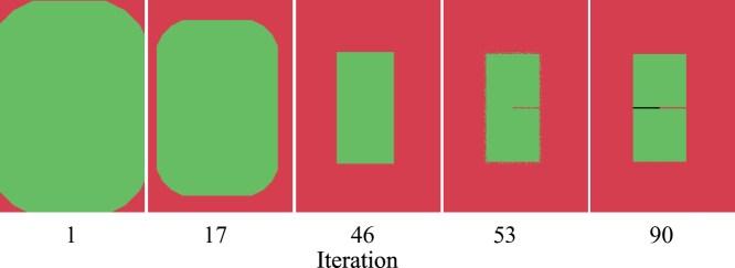
\begin{overpic}[width=216.81pt]{case1.pdf} \end{overpic}

\begin{overpic}[width=216.81pt]{case2.pdf} \put(76.0,66.5){{\scriptsize$\nabla\mathcal{L}_{CE}$}} \put(76.0,59.5){{\scriptsize$\nabla\mathcal{L}_{J}$}} \put(76.0,52.0){{\scriptsize$\nabla\mathcal{L}_{JC}$}} \end{overpic}

Fig. 4: We simulate segmentation towards ground truth by shrinking an initial incorrect segmentation until it shrinkwraps the two target cells (green squares above). This happens while we slowly increase the probabilities of all pixels towards their correct class. During this stage, $\mathcal{L}_{CE}$ drives optimization. Around the shrinkwrap point, $\mathcal{L}_{J}$ dominates the gradient descent as $\nabla\mbox{$\mathcal{L}_{CE}$}\approx 0$ is no longer sufficient to drive the optimization. The ground truth is achieved (one pixel wide notch and touching are identified) thanks to $\nabla\mbox{$\mathcal{L}_{J}$}$ which does not vanish until the segmentation is correct. Cross entropy and $J$ statistic work in tandem. They are not sufficient if used separetely.

\begin{overpic}[width=346.89731pt]{all_landscape.png} \put(12.0,3.0){$\mathcal{L}_{BWM}$} \put(47.0,3.0){$\mathcal{L}_{\text{W}^{3}}$} \put(75.0,3.0){$\mathcal{L}_{JC}$} \end{overpic}

Fig. 5: Loss landscape visualization around a known optimal point $\theta^{*}$ for weighted cross entropy with class balance $\mathcal{L}_{BWM}$ [12], triplex weight map $\mathcal{L}_{\text{W}^{3}}$ [1], and our $\mathcal{L}_{JC}$ loss, all in same scale. Note how the latter would lead to a faster convergence when close to $\theta^{*}$ due to its steep gradients.

 

Loss visualization. We use the approach proposed by Li et al. [20] to help us visualize how our $\mathcal{L}_{JC}$ loss compares to others – $\mathcal{L}_{BWM}$, weighted cross entropy with class balance, and $\mathcal{L}_{\text{W}^{3}}$, triplex weight map [1] – around a known optimal point in the optimization space. As shown in Fig.5, our loss has a cone–like shape whose gradients favor a fast descent to the optimum, contrary to the other losses $\mathcal{L}_{BWM}$ and $\mathcal{L}_{\text{W}^{3}}$ which have near zero gradients all over potentially preventing the optimization to reach the optimum – gradient descent methods are extremely slow to converge in these cases. Although this analysis is based on a visualization that employs dimensionality reduction, our evidences from other experiments suggest this behavior spans the entire optimization space.

Gap assignment. We obtain a semantic segmentation from the output probability map $z$ using the Maximum A Posteriori (MAP) decision rule, $\hat{h}(p)=\arg\max_{l}z_{l}(p)$. A gap pixel $p$, $\hat{h}(p)=3$, can be directly classified as a true background pixel or, in case of dubious probabilities, $z_{0}(p)\approx z_{1}(p)\approx z_{2}(p)$, we assign the second most likely class to it. This is equivalent of applying MAP on the first three classes of the output map, $\hat{h}(p)=\arg\max_{l\in\{0,1,2\}}z_{l}(p)$. An instance segmentation is achieved then by a sequence of labeling operations on each region in the semantic segmentation map [1].

3 Results

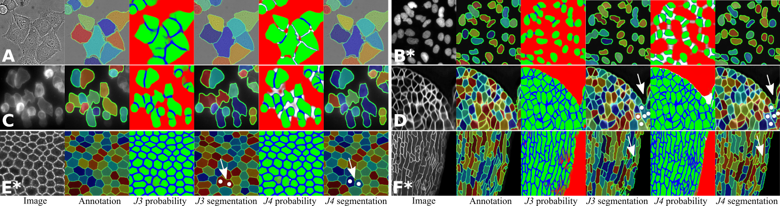
Fig. 6: Segmentation results for Hela cells (A), Hela nuclei (B), T-Cells (C), Arabidopsis thaliana meristematic cells (a YZ-slice of the 3D segmented stack is shown) (D), Drosophila cells (E), and Arabidopsis thaliana sepal cells (z projection) (F) images using networks trained with $J3$ and $J4$ loss functions. Probability maps are shown as RGB images with Background (red), Cell (green), and Touching (blue) classes. For $J4$, the proximity prediction is shown in white. Asterisks (*) indicate zero-shot instance segmentations with networks trained exclusively over T-Cells (C). Colors are to show cell separation. Original images were enhanced to help visualization. Whites arrows and circles are used to indicate some diferences between $J3$ and $J4$.

 

To facilitate comparing our loss $\mathcal{L}_{JC}$ to losses weighted cross entropy with class balance (BWM), weighted cross entropy with triplex weight map (W³) [1], and cross entropy with dice regularization (DSC) [21] we use all with the same U-Net [12], with initial weights following a normal distribution [22], and all equally initialized by fixing all random seeds. For 3D volumes we used 3D convolutions but maintained the same architecture topology as in 2D [5]. A Watershed post-processing (WT) is also applied to those results showing weak touching separation (see [1] for details). The influence of the gap class over training was also analyzed by comparing $J3$ and $J4$ over a DIC Hela dataset [23], a 3D meristem confocal stack (see Fig.7), and T-Cells from [1]. Zero shot segmentation of Hela cells [24] was obtained by using a model trained over the T-Cells data. We used the optimizer Adam [25] with initial learning rate of $10^{-4}$. Data augmentation included random rotation, mirroring, gamma correction, touching contrast modulation [1], and warping. Precision (P05) and F1 score (RQ) were used for cell detection rates. Segmentation Quality (SQ) and Panoptic Quality were, respectively, used for measuring contour adequacy and instance segmentation quality [14].

Instance segmentation performance: Table 1 shows a performance comparison of networks trained with different loss functions. Watershed (WT) post-processing effectively increased the performance of BWM, DSC and W³ when compared with Maximum a Posteriori (MAP). However, the WT method depends on carefully choosing two parameters. Networks trained with the proposed $\mathcal{L}_{JC}$ loss are able to improve instance detection rates using only the parameter-free MAP post-processing. This is due to improvements in the probabilities of gap and touching regions leading to better cell separation. Because we have a weakly annotated ground truth (see annotation in Fig. 1), we found SQ values are not always reliable.

Loss function	Post	P05	RQ	SQ	PQ
BWM	MAP	0.6756	0.5580	0.8674	0.4858
DSC	MAP	0.9028	0.7674	0.9011	0.6923
W3	MAP	0.7384	0.6305	0.8721	0.5513
BWM	WT	0.8193	0.8405	0.8831	0.7437
DSC	WT	0.8726	0.8269	0.8925	0.7390
W3	WT	0.9028	0.8775	0.8995	0.7896
$J3$ (Ours)	MAP	0.9127	0.9069	0.8733	0.7921
$J4$ (Ours)	MAP	0.9334	0.9353	0.8689	0.8132

Table 1: Performance comparison of networks trained over Weighted Cross Entropy with class Balance (BWM), Cross Entropy with Dice regularization (DSC) [21], Weighted Cross Entropy with Triplex weight map (W³) [1], and $\mathcal{L}_{JC}$ over three, $J3$, and four, $J4$, classes.

We use $\mathcal{L}_{JC}$ to assess the gap class influence. Table 2 shows results obtained over each dataset. The best Panoptic Quality, PQ, for all cases was obtained with four classes. An improvement on the Segmentation Quality is observed for the first two datasets, as a direct consequence of using a fourth class (see first row in Fig.6). However, as stated before, weak annotations in the case of T-Cells and meristem datasets tainted SQ values: in reality, a visual inspection shows $J4$ offers a better contour adequacy. The second row of Fig.6 shows examples of $J3$ and $J4$ segmentation and probability maps for T-Cells and meristem volume. Results showed in Figure 6B, E and F were obtained with a network trained over T-Cells images (zero-shot instance segmentation).

Loss function	Dataset	RQ	SQ	PQ
$J3$	DIC	0.8950	0.8547	0.7633
$J4$	DIC	0.8884	0.8833	0.7841
$J3$	HELA*	0.8527	0.8475	0.7237
$J4$	HELA*	0.9046	0.8574	0.7764
$J3$	TCELLS	0.9069	0.8733	0.7921
$J4$	TCELLS	0.9353	0.8689	0.8132
$J3$	MERISTEM 3D	0.8829	0.8820	0.7787
$J4$	MERISTEM 3D	0.8947	0.8804	0.7878

Table 2: Results obtained over different datasets show the benefits of using the additional gap class. In all cases a higher PQ value is obtained for $J4$. A (*) indicates zero-shot segmentation.

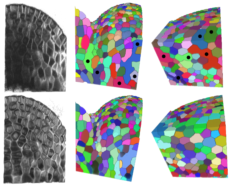
Fig. 7: $\mathbf{J4}$ 3D segmentation of Arabidopsis thaliana meristems. Original and enhanced versions (left column) of a portion of a shoot apical meristem image stack and their respective segmentations (two views on the middle and right columns). Due to space limitation we show only results for this portion which has been previously carefully segmented using the watershed with markers technique, which we consider as an approximate ground truth. Enhancing the signal quality improves segmentation, as shown for those undersegmented regions of the noisy stack manually marked with black circles. Our trained network can process large, 1024x1024x508, meristem stacks in under 9 minutes using 2 Nvidia K80 GPU cards (31 minutes using a single card). Visualizations were prepared using ImageJ 3D Viewer plugin [26].

4 Conclusions

We proposed $JC$ loss, a Youden’s $J$ statistic regularization to the bare cross entropy loss. We build upon our previous work and introduced a new pixel/voxel class we call gap which improves classification and contour adequacy. The approach improved 2D and 3D instance segmentation of highly cluttered cells even after training with weak annotations. Landscape analysis and performance evaluation with different loss functions suggest our new loss is superior to segment cluttered cells. In future work we plan to optimize the proposed pairwise loss to be linear in the number of classes and extensively compare our methods using benchmarks.

References

- [1] Fidel A Guerrero-Peña, Pedro D Marrero Fernandez, Tsang Ing Ren, and Alexandre Cunha, “A weakly supervised method for instance segmentation of biological cells,” in Medical Image Learning with Less Labels and Imperfect Data, MICCAI Workshop, pp. 216–224. Springer, 2019.
- [2] Fidel A Guerrero-Pena, Pedro D Marrero Fernandez, Tsang Ing Ren, Mary Yui, Ellen Rothenberg, and Alexandre Cunha, “Multiclass Weighted Loss for Instance Segmentation of Cluttered Cells,” in 2018 IEEE ICIP. IEEE, 2018, pp. 2451–2455.
- [3] Alexandre Cunha, Paul T Tarr, Adrienne HK Roeder, Alphan Altinok, Eric Mjolsness, and Elliot M Meyerowitz, “Computational analysis of live cell images of the Arabidopsis thaliana plant,” in Methods in Cell Biology, vol. 110, pp. 285–323. Elsevier, 2012.
- [4] Alexandre Cunha, Adrienne HK Roeder, and Elliot M Meyerowitz, “Segmenting the sepal and shoot apical meristem of Arabidopsis thaliana,” in IEEE EMBS International Conference, 2010, pp. 5338–5342.
- [5] Fausto Milletari, Nassir Navab, and Seyed-Ahmad Ahmadi, “V-Net: Fully Convolutional Neural Networks for Volumetric Medical Image Segmentation,” in 2016 Fourth International Conference on 3D Vision (3DV). IEEE, 2016, pp. 565–571.
- [6] Seyed Sadegh Mohseni Salehi, Deniz Erdogmus, and Ali Gholipour, “Tversky Loss Function for Image Segmentation Using 3D Fully Convolutional Deep Networks,” in International Workshop on Machine Learning in Medical Imaging. Springer, 2017, pp. 379–387.
- [7] Maxim Berman, Amal Rannen Triki, and Matthew B Blaschko, “The Lovász-Softmax Loss: A Tractable Surrogate for the Optimization of the Intersection-Over-Union Measure in Neural Networks,” in Proceedings of IEEE CVPR, 2018, pp. 4413–4421.
- [8] Hoel Kervadec, Jihene Bouchtiba, Christian Desrosiers, Eric Granger, Jose Dolz, and Ismail Ben Ayed, “Boundary Loss for Highly Unbalanced Segmentation,” in Proceedings of The 2nd International Conference on Medical Imaging with Deep Learning, 2019, vol. 102, pp. 285–296.
- [9] Tom Brosch, Youngjin Yoo, Lisa YW Tang, David KB Li, Anthony Traboulsee, and Roger Tam, “Deep convolutional encoder networks for multiple sclerosis lesion segmentation,” in MICCAI 2015. Springer, 2015, pp. 3–11.
- [10] Carole H Sudre, Wenqi Li, Tom Vercauteren, Sebastien Ourselin, and M Jorge Cardoso, “Generalised dice overlap as a deep learning loss function for highly unbalanced segmentations,” in Deep Learning in Medical Image Analysis and Multimodal Learning for Clinical Decision Support, pp. 240–248. Springer, 2017.
- [11] William R Crum, Oscar Camara, and Derek LG Hill, “Generalized overlap measures for evaluation and validation in medical image analysis,” IEEE Transactions on Medical Imaging, vol. 25, no. 11, pp. 1451–1461, 2006.
- [12] Olaf Ronneberger, Philipp Fischer, and Thomas Brox, “U-Net: Convolutional Networks for Biomedical Image Segmentation,” in 2015 MICCAI. Springer, 2015, pp. 234–241.
- [13] Dennis Eschweiler, Thiago V Spina, Rohan C Choudhury, Elliot Meyerowitz, Alexandre Cunha, and Johannes Stegmaier, “CNN-based preprocessing to optimize watershed-based cell segmentation in 3D confocal microscopy images,” in 2019 IEEE ISBI. IEEE, 2019, pp. 223–227.
- [14] Alexander Kirillov, Kaiming He, Ross Girshick, Carsten Rother, and Piotr Dollár, “Panoptic Segmentation,” in Proceedings of IEEE CVPR, 2019, pp. 9404–9413.
- [15] William J Youden, “Index for Rating Diagnostic Tests,” Cancer, vol. 3, no. 1, pp. 32–35, 1950.
- [16] Guogen Shan, “Improved Confidence Intervals for the Youden Index,” PloS One, vol. 10, no. 7, pp. e0127272, 2015.
- [17] Sabri Boughorbel, Fethi Jarray, and Mohammed El-Anbari, “Optimal Classifier for Imbalanced Data Using Matthews Correlation Coefficient Metric,” PloS One, vol. 12, no. 6, pp. e0177678, 2017.
- [18] Ian Goodfellow, Yoshua Bengio, and Aaron Courville, “Deep Learning,” MIT Press, 2016.
- [19] Brian W Matthews, “Comparison of the Predicted and Observed Secondary Structure of T4 Phage Lysozyme,” Biochimica et Biophysica Acta (BBA)-Protein Structure, vol. 405, no. 2, pp. 442–451, 1975.
- [20] Hao Li, Zheng Xu, Gavin Taylor, Christoph Studer, and Tom Goldstein, “Visualizing the Loss Landscape of Neural Nets,” in Advances in Neural Information Processing Systems, 2018, pp. 6389–6399.
- [21] Fabian Isensee, Jens Petersen, Andre Klein, David Zimmerer, Paul F Jaeger, Simon Kohl, Jakob Wasserthal, Gregor Koehler, Tobias Norajitra, Sebastian Wirkert, et al., “nnU-Net: Self-adapting Framework for U-Net-Based Medical Image Segmentation,” in Bildverarbeitung für die Medizin, pp. 22–22. Springer, 2019.
- [22] Xavier Glorot and Yoshua Bengio, “Understanding the Difficulty of Training Deep Feedforward Neural Networks,” in Proceedings of the International Conference on Artificial Intelligence and Statistics (AISTATS), 2010, pp. 249–256.
- [23] “ISBI Cell Tracking Challenge: http://celltrackingchallenge.net/2d-datasets/,” 2019, Accessed on 10.07.2019.
- [24] Vebjorn Ljosa, Katherine L Sokolnicki, and Anne E Carpenter, “Annotated High-throughput Microscopy Image Sets for Validation,” Nature Methods, vol. 9, no. 7, pp. 637–637, 2012.
- [25] Diederik P Kingma and Jimmy Ba, “Adam: A Method for Stochastic Optimization,” arXiv:1412.6980, 2014.
- [26] Benjamin Schmid, Johannes Schindelin, Albert Cardona, Mark Longair, and Martin Heisenberg, “A high-level 3D visualization API for Java and ImageJ,” BMC Bioinformatics, vol. 11, no. 1, pp. 274, 2010.