Nonparametric inference of neutron star composition, equation of state,
and maximum mass with GW170817

Abstract

The detection of GW170817 in gravitational waves provides unprecedented constraints on the equation of state (EOS) of the ultra-dense matter within the cores of neutron stars (NSs). We extend the nonparametric analysis first introduced in Landry & Essick (2019), and confirm that GW170817 favors soft EOSs. We infer macroscopic observables for a canonical $1.4\,M_{\odot}$ NS, including the tidal deformability $\Lambda_{1.4}=211^{+312}_{-137}$ ($491^{+216}_{-181}$) and radius $R_{1.4}=10.86^{+2.04}_{-1.42}$ ($12.51^{+1.00}_{-0.88}$) km, as well as the maximum mass for nonrotating NSs, $M_{\mathrm{max}}=2.064^{+0.260}_{-0.134}$ ($2.017^{+0.238}_{-0.087}$)$\,M_{\odot}$, with nonparametric priors loosely (tightly) constrained to resemble candidate EOSs from the literature. Furthermore, we find weak evidence that GW170817 involved at least one NS based on gravitational-wave data alone ($B^{\mathrm{NS}}_{\mathrm{BBH}}=3.3\pm 1.4$), consistent with the observation of electromagnetic counterparts. We also investigate GW170817’s implications for the maximum spin frequency of millisecond pulsars, and find that the fastest known pulsar is spinning at more than 50% of its breakup frequency at 90% confidence. We additionally find modest evidence in favor of quark matter within NSs, and GW170817 favors the presence of at least one disconnected hybrid star branch in the mass–radius relation over a single stable branch by a factor of $2$. Assuming there are multiple stable branches, we find a suggestive posterior preference for a sharp softening around nuclear density followed by stiffening around twice nuclear density, consistent with a strong first-order phase transition. While the statistical evidence in favor of new physics within NS cores remains tenuous with GW170817 alone, these tantalizing hints reemphasize the promise of gravitational waves for constraining the supranuclear EOS.

I Introduction

The observation of gravitational waves (GWs) from GW170817 B. P. Abbott et al. (2017) (LIGO Scientific Collaboration and Virgo Collaboration), a coalescing compact binary with an electromagnetic counterpart, has greatly advanced the study of nuclear matter at extreme densities. Changes in the orbital phasing due to the components’ mutual tidal interaction leave a detectable imprint in the GW signal Hinderer et al. (2010); Read et al. (2013); Del Pozzo et al. (2013); Wade et al. (2014); Damour et al. (2012), and several studies have exploited this fact to infer the tidal deformabilities of the compact objects involved in the coalescence Abbott and et al. (2019a); De et al. (2018); Abbott and et al. (2018); Landry and Essick (2019). Additionally, the observations of counterparts across the electromagnetic spectrum provide complementary constraints on tidal effects Margalit and Metzger (2017); Radice et al. (2018); Radice and Dai (2019); Coughlin et al. (2018). As the advanced LIGO J. Aasi et al. (2015) (LIGO Scientific Collaboration) and Virgo F. Acernese et al. (2015) (Virgo Collaboration) detectors continue to operate, further observations of NS coalescences (e.g. Refs. The LIGO Scientific Collaboration and The Virgo Collaboration (2019a); The LIGO Scientific Collaboration and The Virgo Collaboration (2019b)) will add to our knowledge of the supranuclear equation of state (EOS) Lackey and Wade (2015); McNeil Forbes et al. (2019).

Landry & Essick Landry and Essick (2019) (hereafter LE) recently introduced a nonparametric method for inferring the NS EOS from GW observations based on Gaussian processes that automatically incorporate physical constraints, like causality and thermodynamic stability. We extend their methodology, apply it to GW170817, and obtain updated constraints on the EOS, as well as new bounds on several derived quantities. This includes testing hypotheses about the composition of dense matter and support for hybrid stars for the first time, as well as revisiting the consistency of observed pulsar spins with their rotational breakup frequencies.

LE discussed the advantages of nonparametric analyses over parametric inference schemes with a finite number of parameters. Our updated analysis continues to avoid the kind of modeling systematics inherent to a coarse parametric representation of the EOS’s unknown functional form, and we additionally improve the construction of the nonparametric EOS prior in several ways, reducing the impact of ad-hoc choices made within LE. Whereas LE chose hyperparameters for their Gaussian processes by hand when constructing their priors, we select them by finding hyperparameter sets that optimally reproduce the variability seen in a training set of candidate EOSs. We further sample over a mixture model of such sets, representing the overall process as a weighted sum over many individual Gaussian processes. Our priors, like LE’s, naturally incorporate variable uncertainty in the EOS at different pressures, including tight constraints at low densities, where nuclear matter is better understood, and broader uncertainties at high densities. We also train our Gaussian processes on 50 tabulated candidate EOSs (as opposed to the 7 used in LE) and subdivide the resulting priors according to the composition of the EOSs on which they were trained. This elucidates finer-grained questions about NS composition while incorporating a broader range of theoretical expectations. Moreover, like Ref. Gamba et al. (2019), our analysis marginalizes over several possible crust EOSs to account for the (relatively small) uncertainty in the NS EOS at low densities. Leveraging this, we present new results based on the inferred posterior process for the EOS, including both posterior distributions for macroscopic observables associated with GW170817 itself and functional relations between generic NS observables.

Consistent with previous studies Abbott and et al. (2018); The LIGO Scientific Collaboration and et al. (2019); Landry and Essick (2019); De et al. (2018), we find that GW170817 favors relatively soft EOSs, assuming the system’s components were both slowly spinning NSs Abbott and et al. (2019a). This manifests as an overall posterior preference for lower pressures at and above nuclear density ($\rho_{\mathrm{nuc}}=2.8\times 10^{14}\,\mathrm{g}/\mathrm{cm}^{3}$), as well as smaller radii ($R$), tidal deformabilities ($\Lambda$), and maximum masses for nonrotating NSs ($M_{\mathrm{max}}$). Our results are conditioned on the existence of $\approx 2M_{\odot}$ pulsars Antoniadis et al. (2013); Cromartie et al. (2019) a priori, as we retain only EOSs drawn from our prior that support NSs of at least $1.93\,M_{\odot}$. All our conclusions, then, depend on GW and pulsar data, and our Bayes factors compare our GPs conditioned on both to those conditioned only on pulsar observations. Like LE, we derive results using both model-agnostic and model-informed priors, reflecting different amounts of relative a priori confidence in candidate EOSs from the literature. Our informed prior is conditioned to closely emulate the behavior of EOSs proposed in the literature, whereas our agnostic prior generates much more diverse EOS behavior and is not tightly constrained by the EOS upon which it was conditioned. With the agnostic (informed) prior, we infer median and 90% highest-probability-density credible regions for the macroscopic observables of a canonical 1.4$\,M_{\odot}$ NS: $\Lambda_{1.4}=211^{+312}_{-137}$ ($491^{+216}_{-181}$) and $R_{1.4}=10.86^{+2.04}_{-1.42}$ ($12.51^{+1.00}_{-0.88}$) km, with $M_{\mathrm{max}}=2.064^{+0.260}_{-0.134}$ ($2.017^{+0.238}_{-0.087}$)$\,M_{\odot}$, after marginalizing over EOS composition. These results are broadly consistent with LE and other studies.

By constructing separate priors for different EOS compositions, our updated analysis shows that GW170817 weakly favors EOSs that contain quark matter: $P(\mathrm{Quark}|\mathrm{data})=56\%$ assuming equal prior odds for hadronic, hyperonic, and quark compositions with our informed prior. Remarkably, with the agnostic prior, we find that GW170817 modestly favors EOSs that support a disconnected hybrid star branch, one signature of a strong first-order phase transition. Among such EOSs, GW170817 suggests a possible phase transition with onset density between $\rho_{\mathrm{nuc}}$ and 2$\rho_{\mathrm{nuc}}$, in agreement with chiral effective field theory predictions for the breakdown of perturbations off of asymmetric nuclear matter Tews et al. (2018a, b, 2019); Furnstahl et al. (2015). Our nonparametric inference attaches no a priori significance to these particular densities; the preference observed a posteriori is entirely driven by data from GW170817 and $M_{\mathrm{max}}$ constraints from observations of massive pulsars. While these results are far from conclusive, they demonstrate the extent of information available from GW observations and hint at new physics within NS cores.

We also reexamine limits on NS spin based on the EOS, finding maximum dimensionless spins $\chi_{\mathrm{max}}\lesssim 0.5$ for masses $M\gtrsim M_{\odot}$. We find that the fastest known pulsar, J1748-2446ad Hessels et al. (2006), which does not have a precisely measured mass, rotates at $\gtrsim 1/2$ its breakup frequency for the same mass range at 90% confidence.

We additionally compute the relative marginal likelihoods for different progenitor systems, e.g. binary NS ($\mathrm{BNS}$) vs. NS-black hole ($\mathrm{NSBH}$), finding a preference for progenitor systems containing at least one NS compared to a binary BH ($\mathrm{BBH}$) by a factor of $3.3\pm 1.4$ while making minimal assumptions about the components’ spins, in agreement with the observation of electromagnetic counterparts Abbott and et al. (2017a, b). Interestingly, we find a further slight preference for the lighter component to be a BH, with $B^{\mathrm{NSBH}}_{\mathrm{BNS}}=1.87\pm 0.61$ for our agnostic prior. This is likely due to GW170817 favoring relatively small $\Lambda_{2}$, which is slightly more consistent with a BH ($\Lambda_{2}=0$) than the large $\Lambda_{2}$ required by most NS EOSs.

As with LE, our agnostic and informed results bracket other results in the literature. For example, Ref. Abbott and et al. (2018) constrained the radii of each of GW170817’s components to be $11.9^{+1.4}_{-1.4}$ km, while Ref. De et al. (2018) assumed $R_{1}=R_{2}$ and found a radius of 8.9–13.2 km. Similarly, Ref. Abbott and et al. (2019a) constrained $\tilde{\Lambda}=300^{+420}_{-230}$ and Ref. De et al. (2018) found $\tilde{\Lambda}=222^{+420}_{-138}$ assuming a uniform component mass prior. We infer $\tilde{\Lambda}=245^{+361}_{-160}$ ($572^{+254}_{-212}$) with the agnostic (informed) prior. Although no previous constraints on NS composition are available, we note that Ref. The LIGO Scientific Collaboration and et al. (2019) calculated Bayes factors between $\mathrm{BNS}$ and $\mathrm{BBH}$ models for individual candidate EOSs, with $\ln B^{\mathrm{BNS}}_{\mathrm{BBH}}\lesssim 2$ using a broad mass prior and the majority of candidate EOSs yielding $\ln B^{\mathrm{BNS}}_{\mathrm{BBH}}\sim 0$. This is in good agreement with our agnostic estimate of $\ln B^{\mathrm{BNS}}_{\mathrm{BBH}}(\chi_{i}\leq 0.89)=0.85\pm 0.69$. Where comparable, our findings are generally in good agreement with existing results in the literature. We additionally present a number of novel results, including the first evidence for NS composition and the existence of hybrid-star branches, and revisit spin constraints for rapidly rotating pulsars in light of GW170817.

We review the nonparametric inference introduced in LE in Section II, including descriptions of our improvements. Section II.1 describes the priors constructed for this work. Using publicly available posterior samples LIGO Scientific Collaboration and Virgo Collaboration from a study of GW170817’s source properties Abbott and et al. (2019a), Section III presents a posteriori constraints obtained for macroscopic observables associated with GW170817, such as the component masses and tidal deformabilities, while Section IV presents constraints for relationships between macroscopic observables, applicable to systems besides GW170817. Section V describes our inference over NS compositions, and we conclude in Section VI.

II Nonparametric Inference of the Equation of State

We extend the nonparametric inference based on Gaussian processes (GPs) detailed in LE, and refer readers to that paper for a pedagogical introduction to GPs, their use in our analysis, and associated notation. Nonetheless, we provide a brief overview in what follows.

A GP assumes Gaussian correlations between functional degrees of freedom, described by a mean and covariance. By conditioning a joint process on the observed data and assuming a functional form for the covariance, we obtain a process for infinitely many degrees of freedom based on a finite set of known data, and the complexity of the resulting nonparametric model can naturally scale with the amount of available data. A thorough description is available in Rasmussen and Williams (2006), but the key insight is that the probability distribution of a functional degree of freedom ($f$) given a corresponding abscissa ($x$) and known data ($f_{\ast}$, $x_{\ast}$) is

$$P(f|f_{\ast},x,x_{\ast};\vec{\sigma})=\frac{P(f,f_{\ast}|x,x_{\ast};\vec{\sigma})}{P(f_{\ast}|x_{\ast};\vec{\sigma})}$$ (1)

assuming

$$P(f,f_{\ast}|x,x_{\ast},\vec{\sigma})=\mathcal{N}\big{(}\mu(x_{i}),K(x_{i},x_{j};\vec{\sigma})\big{)},$$ (2)

where $\mu(x_{i})$ is the mean and $K(x_{i},x_{j};\vec{\sigma})$ the covariance of a multivariate normal distribution. $K$ is a function of the hyperparameters $\vec{\sigma}$. We use the squared-exponential kernel

$$K_{\mathrm{se}}(x_{i},x_{j};\sigma,l)=\sigma^{2}\exp\left(-\frac{(x_{i}-x_{j})^{2}}{2l^{2}}\right),$$ (3)

which models correlations between neighboring functional degrees of freedom, the white-noise kernel

$$K_{\mathrm{wn}}(x_{i},x_{j};\sigma_{\mathrm{obs}})=\sigma_{\mathrm{obs}}(x_{i})\delta(x_{i}-x_{j}),$$ (4)

which models uncertainty at each point, and a scaled covariance between input models

$$K_{\mathrm{mv}}(x_{i},x_{j};m)=\\ m^{2}\left(\frac{1}{N_{A}}\sum\limits_{a\in A}C^{(a)}_{ij}\quad+\right.\quad\quad\quad\quad\quad\quad\quad\quad\quad\quad\quad\quad\quad\quad\\ \left.\frac{1}{N_{A}}\sum\limits_{a\in A}\left(\mu^{(a)}_{i}-\bar{\mu}^{(A)}_{i}\right)\left(\mu^{(a)}_{j}-\bar{\mu}^{(A)}_{j}\right)\right)$$ (5)

where $A$ is the set of $N_{A}$ input models, $\mu^{(a)}$ and $C^{(a)}$ are the mean and covariance of the process for model $a$,

$$\bar{\mu}^{(A)}_{i}=\frac{1}{N_{A}}\sum\limits_{a\in A}\mu^{(a)}_{i},$$ (6)

and $m$ scales the relative importance of this model covariance. $K_{\mathrm{mv}}$, like $K_{\mathrm{wn}}$, represents theoretical uncertainty. We note that LE used a simplified version of $K_{\mathrm{mv}}$ which only included the diagonal components of the covariance matrix.

We generate GPs for an auxiliary variable

$$\phi=\log\left(c^{2}\frac{d\varepsilon}{dp}-1\right)$$ (7)

conditioned on tabulated EOSs from the literature, where $\varepsilon$ is the total energy density and $p$ the pressure. Any realization of $\phi$ will automatically satisfy both causality and thermodynamic-stability constraints ($0\leq c_{s}^{2}=dp/d\varepsilon\leq c^{2}$). Our method employs GPs for two main purposes: mapping irregularly sampled tabulated data for $\varepsilon(p)$ into a regularly sampled process for $\phi(p)$ while self-consistently computing the uncertainty in that mapping, and emulating the behavior seen in tabulated EOSs to generate synthetic EOSs which resemble models from the literature. This work differs from LE in that we construct mixture models of GPs instead of relying on a single set of hyperparameters. That is,

$$\phi\sim\sum\limits_{i}w_{i}P(\phi|\vec{\sigma}_{i})$$ (8)

where $\vec{\sigma}_{i}$ and $w_{i}$ are the hyperparameters and weight associated with the $i^{\mathrm{th}}$ element of the mixture model.

We constrain our processes to approximately match known low-pressure physics with an additional white-noise variant. This forces all realizations of the conditioned process to approach a constant value (chosen to be $\phi\rightarrow\phi_{0}=6$ based on sly Douchin and Haensel (2001)) with a white-noise scaling parameter

$$\sigma_{\mathrm{obs}}(p)=\left(\frac{p}{p_{\mathrm{ref}}}\right)^{n}.$$ (9)

At low pressures, $\sigma_{\mathrm{obs}}\rightarrow 0$, forcing the conditioned process to approach $\phi_{0}$ while imposing no constraint when $p\gg p_{\mathrm{ref}}$. Here we set $p_{\mathrm{ref}}=5.4\times 10^{31}\,\mathrm{dyn}/\mathrm{cm}^{2}$ and $n=5$, ad hoc choices with negligible impact on the resulting EOS, as we match the GP realizations onto a fixed model for the low-density crust well above $p_{\rm ref}$. Improved matching conditions that incorporate the expected uncertainty from first-principles theoretical calculations, such as those in Refs. Furnstahl et al. (2015); Hebeler et al. (2013); Tews et al. (2013, 2018a), may further enhance our analysis. Similarly, matching to known high-density behavior, like $c_{s}^{2}\rightarrow c^{2}/3$ for hyperrelativistic matter Fraga et al. (2016); Kurkela et al. (2014), could prove interesting. However, we leave this to future work.

In addition to these technical improvements, we extend LE’s analysis by conditioning our GPs on more tabulated EOSs (50 instead of 7) with a broader range of phenomenology and compositions. We also subdivide our agnostic and informed priors according to the composition of the input candidate EOSs (hadronic $npe\mu$ matter, hyperonic $npe\mu{Y}$ matter, or $npe\mu(Y)Q$ quark matter) allowing for model selection between different NS constituents.

II.1 Constructing nonparametric priors

We construct several priors using the candidate EOSs listed in Table 7. In order to fairly weight the importance of each input EOS, we group them by composition and underlying family of nuclear effective forces, generating representative processes for each family separately and then weighting the resulting GPs equally. This is done hierarchically in order to synthesize overarching agnostic and informed priors, as well as priors that demonstrate behavior characteristic of EOSs with a particular composition.

We map $\varepsilon$ to $\phi$ for each EOS, modeling each one’s covariance matrix separately with a squared-exponential kernel with a small white-noise term ($\sigma\gg\sigma_{\mathrm{obs}}$), and then generate a sequence of overarching GPs which emulate the behavior observed between different EOSs using a combination of squared-exponential, white-noise, and model covariance kernels. As in LE, we take the mean of the joint process before conditioning to be a low-order polynomial fit to the input data.

We optimize the hyperparameters used to generate our priors with a cross-validation likelihood

$$P_{\mathrm{CV}}(\{\varepsilon\}_{A}|p,\vec{\sigma})=\prod\limits_{a\in A}P(\varepsilon^{(a)}|\{\varepsilon\}_{A\setminus a},p,\vec{\sigma}),$$ (10)

where $\{\varepsilon\}_{A}$ is the set of all EOSs and $\{\varepsilon\}_{A\setminus a}$ is the set of all EOSs in $A$ except $\varepsilon^{(a)}$, and obtain processes that emulate the behavior seen within each composition separately. However, instead of selecting a single set of optimal hyperparameters for each composition, we instead create mixture models by drawing many sets of hyperparameters from $P_{\mathrm{CV}}$ so that

$$P(\varepsilon|\{\varepsilon\}_{A},p)\\ \propto\int d\vec{\sigma}\,P(\vec{\sigma})P_{\mathrm{CV}}(\{\varepsilon\}_{A}|\vec{\sigma})^{\beta}P(\varepsilon|\{\varepsilon\}_{A},p,\vec{\sigma})\\ \approx\left.\frac{1}{N}\sum\limits_{i}P_{\mathrm{CV}}(\{\varepsilon\}_{A}|\vec{\sigma}_{i})^{\beta}P(\varepsilon|\{\varepsilon\}_{A},p,\vec{\sigma}_{i})\quad\right|\quad\vec{\sigma}_{i}\sim P(\vec{\sigma})$$ (11)

where $\beta=1/T$ is an inverse temperature.

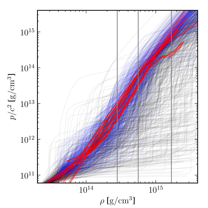
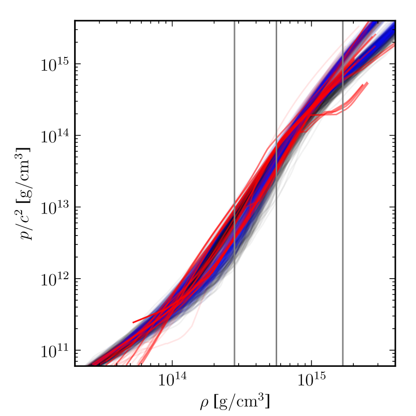
In the limit $T\rightarrow 1$, we weight each set of hyperparameters by the cross-validation likelihood. We call the resulting GP-mixure model the model-informed prior. In the limit $T\rightarrow\infty$, we weight each set of hyperparameters equally, subject to the hyperprior $P(\vec{\sigma})$. This produces a process much less constrained by the input EOSs, which we refer to as the model-agnostic prior. We sample logarithmically in $\sigma$, $\sigma_{\mathrm{obs}}$, and $m$ while sampling linearly in $l$. The precise choice of $P(\vec{\sigma})$ does not strongly affect the model-informed prior, but can modify the behavior of the model-agnostic prior. It is also worth noting that $\beta$ provides a natural way to tune the a priori degree of belief placed on published theoretical models, and our choices for the informed and agnostic priors are not the only ones possible. Example synthetic EOSs are shown Figure 1.

model-agnostic

model-informed

Figure 1: Example synthetic EOSs drawn from our (left) agnostic and (right) informed nonparametric priors, constructed as mixture models with equal prior odds for hadronic, hyperonic, and quark compositions. Draws from the prior are colored according to the maximum nonrotating NS mass they support: blue for $M_{\mathrm{max}}$$\,\geq$ 1.93$\,M_{\odot}$, and black otherwise. Candidate EOSs from the literature, used as input for our GPs, are shown in red (see Table 7). Vertical lines indicate once, twice and six times nuclear saturation density.

II.2 Sampling from nonparametric priors

We obtain a large number of synthetic EOSs by sampling from each process for $\phi$. We integrate each realization $\phi^{(\alpha)}(p)$ to obtain the associated synthetic EOS $\varepsilon^{(\alpha)}(p)$. This includes setting the initial value for the integration, which is done by matching to a crust EOS at a particular pressure. To marginalize over the (relatively small) theoretical uncertainty in the microscopic description of the crust, we randomly match each $\varepsilon^{(\alpha)}$ to the low-density model used in one of either sly Douchin and Haensel (2001), eng Engvik et al. (1996), or hqc18 Baym et al. (2019). Furthermore, the precise pressure at which we match the crust EOS is allowed to vary by approximately an order of magnitude. This procedure generates EOSs which span all densities relevant for NS structure.

We integrate each synthetic EOS to obtain the corresponding relationships between macroscopic observables, such as the mass, radius, and tidal deformability. As in LE, we additionally require that each $\varepsilon^{(\alpha)}$ support at least a $1.93\,M_{\odot}$ star based on the existence of massive pulsars (J0348+0432 Antoniadis et al. (2013)), discarding any synthetic EOS that does not. We also discard any EOS that supports a spurious branch of NSs with $M\gtrsim M_{\odot}$ at subnuclear densities $\rho_{c}<0.8\rho_{\mathrm{nuc}}$, so as to exclude particularly large excursions in pressure just above the crust-core interface. We obtain marginal likelihoods, posterior distributions, and posterior processes by Monte-Carlo sampling from the prior, weighting each sample with a Gaussian kernel density estimate (KDE) for the GW likelihood generated with publicly available samples LIGO Scientific Collaboration and Virgo Collaboration :

$$P(d|\varepsilon^{(\alpha)},\mathcal{H}) =\int dM_{1}dM_{2}\,p(M_{1},M_{2}|\mathcal{H})\,\mathcal{L}\left(\mathrm{data}\left|M_{1},M_{2},\Lambda^{(\alpha)}(M_{1}),\Lambda^{(\alpha)}(M_{2})\right.\right)$$ (12)

$$\approx\frac{1}{N_{i}}\sum\limits_{i}^{N_{i}}\mathcal{L}\left(\mathrm{data}\left|M_{1}^{(i)},M_{2}^{(i)},\Lambda^{(\alpha)}(M_{1}^{(i)}),\Lambda^{(\alpha)}(M_{2}^{(i)})\right.\right)\quad\left|\quad M_{1}^{(i)},M_{2}^{(i)}\sim P(M_{1},M_{2}|\mathcal{H})\right.,$$ (13)

where $\Lambda^{(\alpha)}$ is the mass-tidal deformability relation implicitly defined by $\varepsilon^{(\alpha)}$. It is worth noting that several sets of samples are publicly accessible. Our specific choice is not expected to significantly affect our conclusions, although our precise quantitative results will depend on issues like waveform systematics discussed in Ref. Abbott et al. (2019). Drawing $\varepsilon^{(\alpha)}$ from our prior and associating this marginal likelihood with each sample generates the posterior process. This also allows us to immediately estimate the evidence for each prior, up to a common normalization constant:

$$P(d|\{\varepsilon\}_{A},\mathcal{H})\approx\frac{1}{N_{\alpha}}\sum\limits_{\alpha}^{N_{\alpha}}\frac{1}{N_{i}}\sum\limits_{i}^{N_{i}}\mathcal{L}\left(\mathrm{data}\left|M_{1}^{(i)},M_{2}^{(i)},\Lambda^{(\alpha)}(M_{1}^{(i)}),\Lambda^{(\alpha)}(M_{2}^{(i)})\right.\right)\quad\left|\quad\begin{matrix}M_{1}^{(i)},M_{2}^{(i)}\sim P(M_{1},M_{2}|\mathcal{H})\\ \varepsilon^{(\alpha)}\sim P(\varepsilon|\{\varepsilon\}_{A})\end{matrix}\right.,$$ (14)

where we draw $N_{i}$ mass realizations for each of the $N_{\alpha}$ EOS realizations. Within this Monte-Carlo algorithm, we optimize our KDE model for $\mathcal{L}(d|\cdots)$ by selecting bandwidths that maximize a cross-validation likelihood based on the public samples (see Appendix B).

The overarching composition-marginalized priors are constructed hierarchically, assuming equal prior odds for each composition, which is to say

$$P(\mathrm{data}|X)=\\ \frac{1}{3}\big{[}P(\mathrm{data}|X;\mathrm{Hadronic})\quad\quad\\ \quad\quad+P(\mathrm{data}|X;\mathrm{Hyperonic})\\ +P(\mathrm{data}|X;\mathrm{Quark})\big{]}$$ (15)

for informed and agnostic priors processes separately. In the following sections, we analyze GW170817 using both our agnostic and informed priors. The full set of results, broken down by composition, is given in Appendix D.

III Implications for GW170817

We apply publicly available GW data from GW170817 LIGO Scientific Collaboration and Virgo Collaboration to our priors to infer the system’s properties a posteriori. Section III.1 focuses on macroscopic observables associated with the inspiral stage of the coalescence, such as component masses ($M_{1,2}$), tidal deformabilities ($\Lambda_{1,2}$), and radii ($R_{1,2}$), while Section III.2 focuses on the nature of the progenitor system and the remnant. Throughout this section, we quote medians and 90% highest-probability-density credible regions unless otherwise stated.

III.1 Constraints on GW170817’s macroscopic observables

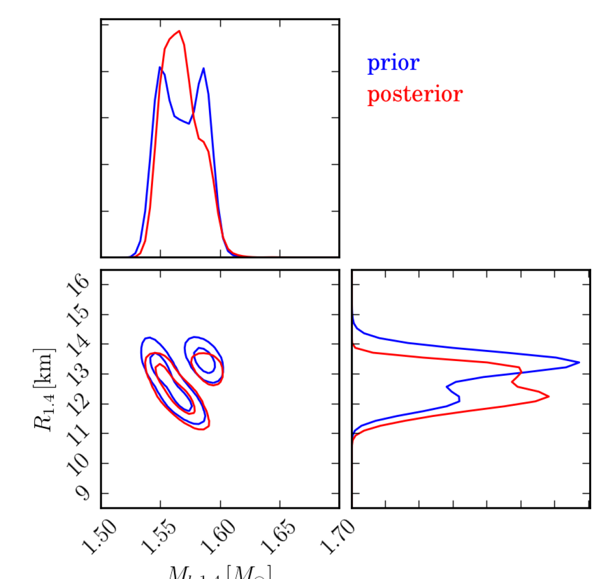
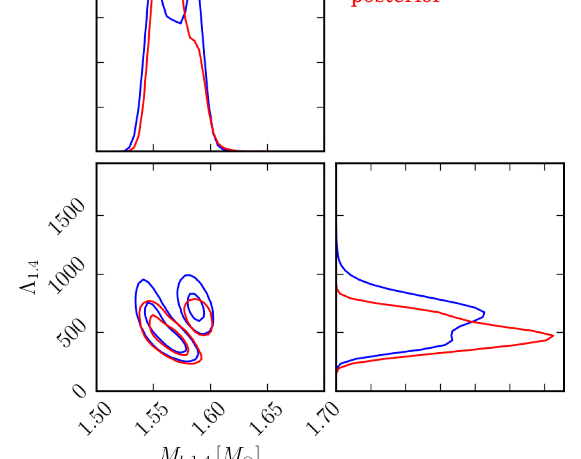
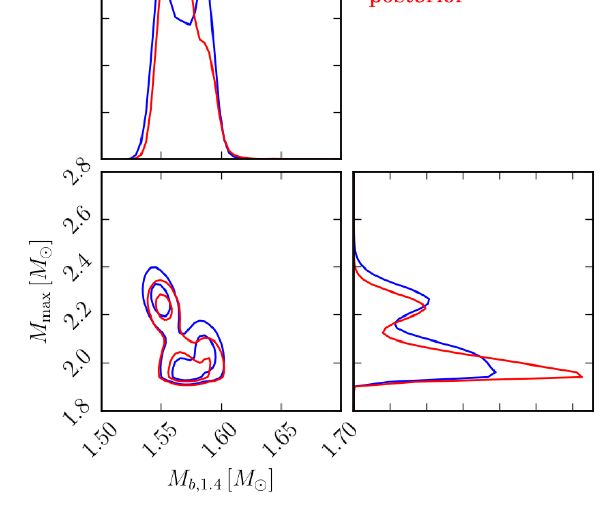
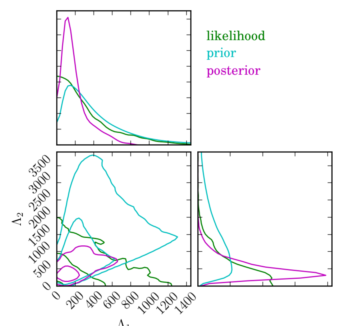
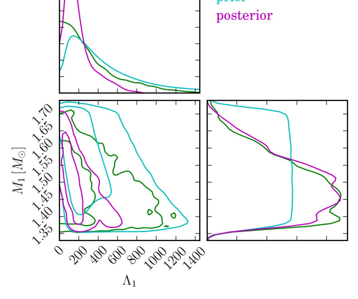
We begin with posterior constraints on the macroscopic properties of GW170817, assuming both compact objects were slowly spinning NSs. Table 1 enumerates credible regions for various properties of GW170817’s constituents, and Figure 2 demonstrates the correlations between some of these properties. In principle, our inference constrains any EOS-dependent observable associated with the event, but we focus on those that either directly impact the GW waveform or have been discussed extensively elsewhere in the literature. While we show low-dimensional projections of our data, we perform our inference in the four-dimensional space spanned by $M_{1}$, $M_{2}$, $\Lambda_{1}$, and $\Lambda_{2}$, and therefore posterior constraints may not be intuitive from the the low-dimensional projections in our figures.

model-agnostic

model-informed

Figure 2: Distributions for $M_{1}$, $\Lambda_{1}$, and $\Lambda_{2}$ after marginalizing over NS composition. (Left) model-agnostic prior (cyan), posterior (magenta), and low-spin marginal likelihood (green). (Right) model-informed prior (blue), posterior (red), and low-spin marginal likelihood (green). Contours in the joint distributions denote highest-posterior-density 50% and 90% credible regions.

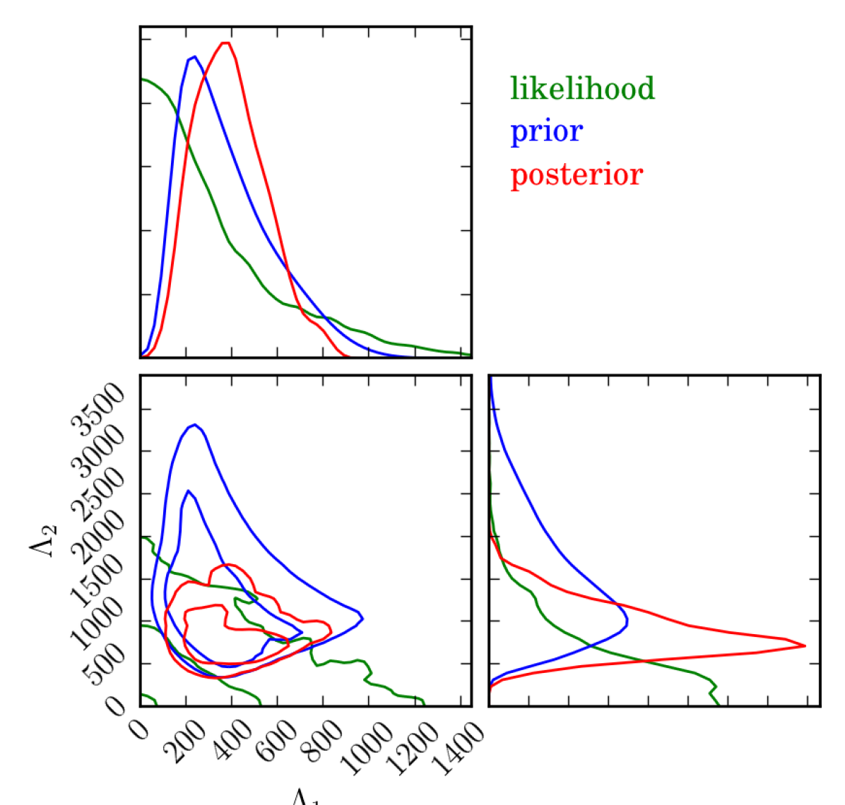
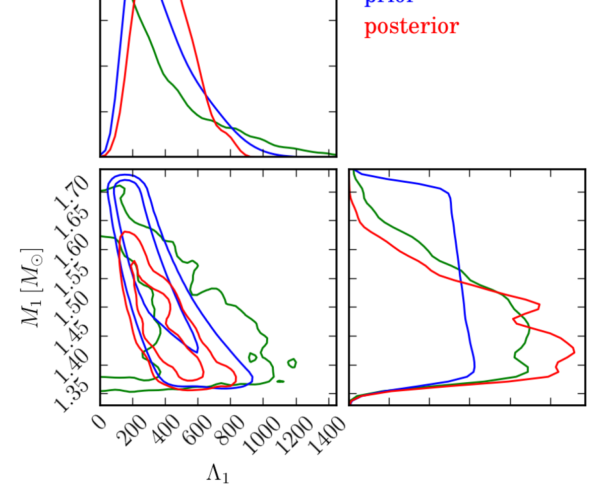
We analyze publicly available posterior samples  with component spins constrained to be below $0.05$ LIGO Scientific Collaboration and Virgo Collaboration , and $\gtrsim O(10^{5})$ synthetic EOSs drawn from each of our priors with 50 mass realizations per EOS. We find that relative uncertainties obtained with the informed prior are generally smaller than those with the agnostic prior, although the distributions of some parameters, like tidal deformabilities, are centered on larger values with the informed prior and can produce larger credible intervals in absolute terms. The inferred component mass distributions do not depend strongly on the EOS prior assumed, although they do change slightly a posteriori because they are correlated with the tidal deformability and radius, which are more sensitive to EOS assumptions. Specifically, the agnostic prior supports extreme EOSs and produces rather low values for $\Lambda$ and $R$ a posteriori. The informed prior prefers stiffer EOSs and yields correspondingly larger $\Lambda$ and $R$. Table 1 lists the precise credible regions obtained. We note that the inferred tidal deformabilities are consistent with LE, and both the $\Lambda$ and $R$ credible regions are consistent with others in the literature. In particular, Ref. Abbott and et al. (2018) constrained $R_{1}$ and $R_{2}$ separately, finding both to be $11.9^{+1.4}_{-1.4}$ km, while Ref. De et al. (2018) assumed a common radius for the NSs and constrained it to 8.9–13.2 km. We find $R_{1}=10.88^{+1.99}_{-1.37}$ km and $R_{2}=10.82^{+2.14}_{-1.55}$ km with our agnostic prior, confirming the validity of the common radius assumption a posteriori. Similarly, Ref. Abbott and et al. (2019a) finds $\tilde{\Lambda}=300^{+420}_{-230}$, while Ref. De et al. (2018) quotes $\tilde{\Lambda}=222^{+420}_{-138}$ for a uniform component mass prior. Our agnostic prior yields $\tilde{\Lambda}=245^{+361}_{-160}$ . Finally, our constraints remain marginally consistent with those quoted in Refs. Radice et al. (2018); Radice and Dai (2019); Margalit and Metzger (2017); Coughlin et al. (2018) based on electromagnetic observations, which set a lower bound of $\tilde{\Lambda}\gtrsim 300$.

Like Figure 1 in Ref. Abbott and et al. (2018) and Figure 6 in LE, Figure 2 shows the prior, likelihood, and posterior credible regions for $M_{1}$, $\Lambda_{1}$, and $\Lambda_{2}$ with our composition-marginalized priors. The preference for softer EOSs in the agnostic prior, both a priori and a posteriori, is readily apparent, as is the fact that the agnostic prior encompasses a wider range of possibilities than the informed prior.

Table 1: Medians a posteriori and highest-probability-density 90% credible regions for macroscopic observables and central densities associated with GW170817.

Prior ($\mathcal{H}_{i}$)	$M_{1}\,[M_{\odot}]$	$M_{2}\,[M_{\odot}]$	$\Lambda_{1}$	$\Lambda_{2}$	$\tilde{\Lambda}$	$R_{1}\,[\mathrm{km}]$	$R_{2}\,[\mathrm{km}]$	$\rho_{c,1}\,[10^{14}\,\mathrm{g}/\mathrm{cm}^{3}]$	$\rho_{c,2}\,[10^{14}\,\mathrm{g}/\mathrm{cm}^{3}]$
informed	$1.46^{+0.11}_{-0.10}$	$1.28^{+0.08}_{-0.09}$	$380^{+249}_{-231}$	$844^{+553}_{-405}$	$572^{+254}_{-212}$	$12.50^{+0.98}_{-0.87}$	$12.51^{+1.02}_{-0.96}$	$7.43^{+1.48}_{-1.23}$	$6.65^{+1.03}_{-1.04}$
agnostic	$1.49^{+0.13}_{-0.13}$	$1.25^{+0.10}_{-0.10}$	$148^{+274}_{-125}$	$430^{+519}_{-301}$	$245^{+361}_{-160}$	$10.88^{+1.99}_{-1.37}$	$10.82^{+2.14}_{-1.55}$	$9.79^{+3.21}_{-3.72}$	$8.85^{+2.52}_{-3.18}$

Table 1 also reports credible intervals for the central densities of the two components. These are consistent with those reported in both LE and Ref. Abbott and et al. (2018). We again note the general trend that the agnostic prior prefers softer EOSs with correspondingly compact stars containing denser cores and higher central pressures.

As discussed in LE, we obtain different a posteriori credible regions with different priors. However, neither of our priors are strongly favored by the data, with a Bayes Factor of $B^{\mathcal{A}}_{\mathcal{I}}=1.7952\pm(1.1\times 10^{-3})$ between them. This constitutes marginal evidence in favor of the agnostic priors over the informed priors, but serves mainly to demonstrate that posterior constraints on macroscopic observables and the EOS need to be interpreted with care, giving consideration to the underlying prior assumptions.

III.2 Implications for GW170817’s progenitor and remnant

Section III.1’s results implicitly assume both constituents are NSs. This is reasonable given the masses involved, which are well below the minimum $M_{\mathrm{max}}$ allowed in our priors, and the electromagnetic counterparts observed in coincidence Abbott and et al. (2017a, b). However, we also consider the possibility that either (or both) of the constituents could be a BH. Although credible regions similar to Section III.1 could be derived for each case, we simply focus on the evidence for each progenitor type to determine whether the GW data alone can rule out the presence of at least one BH in the system.

Our evidence calculation involves Monte-Carlo integrals over a KDE representation of $\mathcal{L}(d|\cdots)$ along boundaries where $\Lambda_{1}$, $\Lambda_{2}\rightarrow 0$. Such boundaries can introduce biases in the KDE representation of $\mathcal{L}$. After optimizing our KDE, we find that these effects introduce percent-level systematics.

We begin by investigating the nature of the progenitor system: did it consist of two NSs (BNS), a NS and a lighter BH ($\mathrm{NSBH}$), a NS and a heavier BH ($\mathrm{BHNS}$), or two BHs ($\mathrm{BBH}$)? Table 2 quotes the posterior probability of each progenitor type assuming equal prior odds. We include results assuming both the low- and high-spin priors from Ref. Abbott and et al. (2019a), although the low-spin prior is motivated by the maximum observed rotation frequencies of pulsars in galactic $\mathrm{BNS}$ systems that will merge within a Hubble time (J0737–3039A Lyne et al. (2004) and J1946+2052 Stovall et al. (2018)) and may not be applicable to BHs. We also test for the presence of at least one NS. We find that GW170817 is relatively inconsistent with a $\mathrm{BBH}$ based on GW data alone, disfavored by a factor of $3.3\pm 1.4$ relative to a progenitor with at least one NS with the high-spin agnostic prior, assuming $P(\mathrm{BNS})=P(\mathrm{NSBH})=P(\mathrm{BHNS})=1/6$ and $P(\mathrm{BBH})=1/2$. The weak preference for the $\mathrm{BNS}$ model with our agnostic prior is likely due to the relatively large Occam factor incurred by the extra freedom associated with $\Lambda_{1,2}$ compared to the $\mathrm{BBH}$ model. Therefore, even though the maximum likelihood within the $\mathrm{BNS}$ model is consistently four times larger than in the $\mathrm{BBH}$ model, the marginal likelihoods are comparable. This is also true to a lesser extent with the informed prior, but its stricter a priori assumptions also reduce the maximum likelihood and therefore the marginal evidence for the $\mathrm{BNS}$ model. In addition, of the possible progenitors containing a NS, GW170817 data weakly favor a NSBH, with $B^{\mathrm{NSBH}}_{\mathrm{BNS}}(\chi_{i}\leq 0.89,\,\text{\emph{agnostic}})=1.87\pm 0.61$. This is likely due to marginally better matches to the data when $\Lambda_{2}\rightarrow 0$ compared to the larger $\Lambda(M_{2})$ required by our priors, instead of just an Occam factor, since $\mathrm{NSBH}$ models are preferred over $\mathrm{BHNS}$ models despite both having approximately equal prior volumes. We obtain qualitatively similar results with the high- and low-spin priors.

Ref. The LIGO Scientific Collaboration and et al. (2019) computed similar Bayes factors for individual tabulated EOSs, finding $\ln B^{\mathrm{BNS}}_{\mathrm{BBH}}\lesssim 2$ for their wide mass prior, with the majority of EOSs considered yielding $\ln B^{\mathrm{BNS}}_{\mathrm{BBH}}\sim 0$, in good agreement with our $\ln B^{\mathrm{BNS}}_{\mathrm{BBH}}(\chi_{i}\leq 0.89,\,\text{\emph{agnostic}})=0.85\pm 0.69$.

Our calculations demonstrate that GW170817 is more consistent with a system containing at least one NS as compared to a $\mathrm{BBH}$. Of course, this result is unsurprising given that an electromagnetic counterpart was observed. Given this, we predict the amount of matter available outside the remnant, similar in spirit to Refs. Coughlin et al. (2018) and Abbott and et al. (2017c), among others Abbott and et al. (2017a); Kasen et al. (2017); Cowperthwaite et al. (2017); Villar et al. (2017); The LIGO Scientific Collaboration and et al. (2019). Using the fitting formula reported in the appendix of Ref. Coughlin et al. (2018), which depends primarily on stellar compactness, we estimate the amount of dynamical ejecta and its velocity, finding $M_{\mathrm{ejecta}}^{(\mathrm{dyn})}=6.5^{+6.3}_{-3.9}\times 10^{-3}$ ($3.9^{+2.4}_{-1.3}\times 10^{-3}$) $M_{\odot}$ and $v_{\mathrm{ejecta}}^{(\mathrm{dyn})}/c=0.257^{+0.027}_{-0.034}$ ($0.231^{+0.014}_{-0.014}$) with our agnostic (informed) prior, generally in good agreement with estimates of the contribution of dynamical ejecta in the literature. We note that our error bars account for the residual EOS uncertainty, but modeling systematics associated with Ref. Coughlin et al. (2018)’s fit surely contribute to the error budget as well. As has been previously noted, this suggests the dynamical ejecta were only a small part of the total ejecta of $\gtrsim 0.05\,M_{\odot}$ which powered GW170817’s kilonova Coughlin et al. (2018); Abbott and et al. (2017c).

Numerical relativity simulations typically do not extend far enough past merger to observe mass ejected via disk winds, which are expected to dominate the total ejected mass. Similarly, it is difficult to estimate the lanthanide fraction, which determines the opacity of the ejected material and the kilonova’s color, from first principles based on $M_{1}$, $M_{2}$, and the EOS. However, were such models available, our posterior processes would immediately bound the expected kilonova properties, just as we already constrain the contribution of dynamical ejecta.

Table 2: Posterior probabilities for progenitor systems assuming equal prior odds. We compare the evidence for a binary NS ($\mathrm{BNS}$), a $\mathrm{NSBH}$ ($M_{1}$ is a NS), a $\mathrm{BHNS}$ ($M_{1}$ is a BH), and a binary BH ($\mathrm{BBH}$). Monte-Carlo sampling uncertainties are approximately three orders of magnitude smaller than the point estimates. Reported uncertainties approximate systematic error from our KDE model of the GW likelihood, which is largest for the $\mathrm{BBH}$ hypothesis.

Spin Prior	EOS Prior ($\mathcal{H}_{i}$)	$P(\mathrm{BNS}|\mathrm{data};\mathcal{H}_{i})$	$P(\mathrm{BHNS}|\mathrm{data};\mathcal{H}_{i})$	$P(\mathrm{NSBH}|\mathrm{data};\mathcal{H}_{i})$	$P(\mathrm{BBH}|\mathrm{data};\mathcal{H}_{i})$
$|\chi_{i}|\leq 0.05$	informed	$(14.3\pm 4.5)\%$	$(23.6\pm 0.5)\%$	$(54.4\pm 1.2)\%$	$(7.8\pm 2.7)\%$
	agnostic	$(25.9\pm 7.1)\%$	$(27.6\pm 1.8)\%$	$(38.3\pm 2.2)\%$	$(8.1\pm 3.1)\%$
$|\chi_{i}|\leq 0.89$	informed	$(11.2\pm 3.7)\%$	$(18.1\pm 0.1)\%$	$(61.0\pm 0.3)\%$	$(9.7\pm 3.3)\%$
	agnostic	$(23.9\pm 6.9)\%$	$(25.2\pm 1.4)\%$	$(40.4\pm 1.7)\%$	$(10.5\pm 3.9)\%$

IV Implications for Neutron Star Properties

In addition to examining the inferred properties of GW170817, we can use the GW data to inform our knowledge of NSs in general. Specifically, we compute posterior processes for various functional degrees of freedom, including the EOS itself and several derived relations between macroscopic observables. If all NSs share a single universal EOS, then these results are immediately applicable to other systems. Tight constraints on these relationships imply consistency tests of the universal-EOS hypothesis with observations of other systems Landry and Kumar (2018); Kumar and Landry (2019). Tables 3 and 4 summarize our conclusions, and we discuss a few salient points in more detail below. As in Section III, we report medians and 90% highest-probability-density credible regions unless otherwise noted.

IV.1 Posterior processes for the EOS

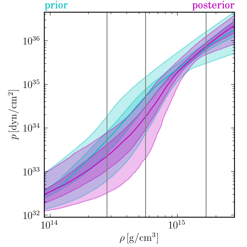
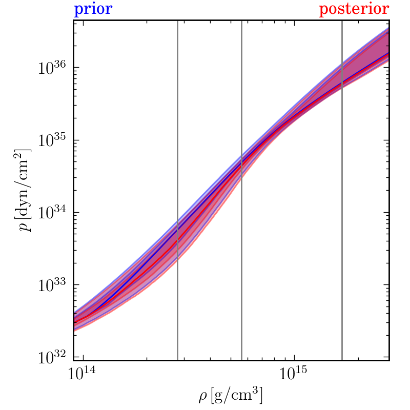
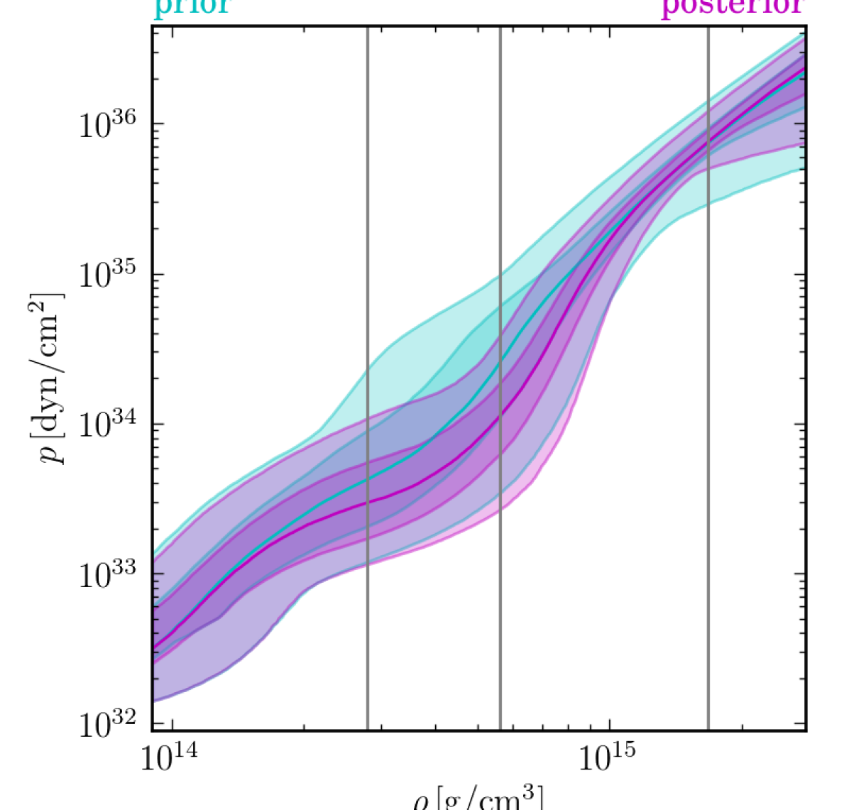
We begin with an inference of the EOS itself, as shown in Figure 3. A posteriori, we observe a general trend towards lower pressures, particularly between $\rho_{\mathrm{nuc}}$ and 2$\rho_{\mathrm{nuc}}$, with a trend back towards pressures near the a priori median at higher densities. Table 3 quantifies the uncertainty in pressure at a few reference densities.

The constraints we obtain are slightly different than, but consistent with, those reported in LE, which is expected from the differences in our GP prior processes. Our agnostic and informed results bracket those reported in Ref. Abbott and et al. (2018)’s parametric analysis, namely $p(2\rho_{\mathrm{nuc}})=3.5^{+2.7}_{-1.7}\times 10^{34}$ dyn/cm² and $p(6\rho_{\mathrm{nuc}})=9.0^{+7.9}_{-2.6}\times 10^{35}$ dyn/cm². Specifically, our agnostic results are systematically lower a posteriori than Ref. Abbott and et al. (2018)’s, while our informed pressure bounds are centered above Ref. Abbott and et al. (2018) at 2$\rho_{\mathrm{nuc}}$. At 6$\rho_{\mathrm{nuc}}$, however, our informed process lies below both Ref. Abbott and et al. (2018) and our agnostic results, although the uncertainties are broad. This inversion likely occurs because GW170817 has little constraining power at high densities, but the informed results favor the presence of quark matter, which systematically softens a priori in this regime.

The trend toward low pressures between $\rho_{\mathrm{nuc}}$ and 2$\rho_{\mathrm{nuc}}$ is likely driven by at least two factors. First, the NS radius and tidal deformability are known to correlate strongly with the pressure in that region Lattimer and Prakash (2001); Read et al. (2009), and therefore GW170817’s preference for small $\Lambda$ manifests as a preference for lower pressures in this region. However, GW170817’s component masses likely have central densities below $10^{15}\,\mathrm{g}/\mathrm{cm}^{3}$, and therefore the GW data only contains information about the EOS at densities lower than this. At significantly higher densities, then, the EOS posterior will tend to snap back towards the prior. That tendency is compounded by the requirement that all EOSs support $1.93\,M_{\odot}$ stars, which forces initially soft EOSs to stiffen at higher densities in order to support massive stars.

model-agnostic

model-informed

Figure 3: EOS processes after marginalizing over composition. (Left) model-agnostic prior (cyan) and posterior (magenta) processes. (Right) model-informed prior (blue) and posterior (red) processes. Shaded regions correspond to 50% and 90% symmetric marginal credible regions for the pressure at each density. Solid lines denote the median and vertical lines denote $\rho_{\mathrm{nuc}}$, 2$\rho_{\mathrm{nuc}}$, and 6$\rho_{\mathrm{nuc}}$.

IV.2 Posterior distributions and processes for macroscopic observables

model-agnostic

Figure 4: Processes relating a few macroscopic observables after marginalizing over EOS composition with the agnostic prior. Prior (cyan) and posterior (magenta) processes for (left) tidal deformability ($\Lambda$; top), radius ($R$; middle), and moment of inertia ($I$; bottom) as functions of mass as well as (right) the maximum spin frequency ($f_{\mathrm{max}}$; top), maximum dimensionless spin parameter ($\chi_{\mathrm{max}}$; middle), and the dimensionless spin parameter divided by the spin frequency (bottom), useful when estimating $\chi$ for a pulsar with unknown mass. Shaded regions denote the 50% and 90% symmetric credible regions for the marginal distribution of each observable at each mass. Solid lines denote the median and vertical lines denote canonical $1.4\,M_{\odot}$ stars. Horizontal grey lines in the top-right panel denote the measured spin frequencies of J1748–2446ad ($716\,\mathrm{Hz}$ Hessels et al. (2006)) and B1937+241 (641 Hz Backer et al. (1982)), which lie below the 90% lower limits for $f_{\mathrm{max}}$ only when $M\gtrsim M_{\odot}$.

Table 3: Medians a posteriori and highest-probability-density 90% credible regions for a canonical $1.4\,M_{\odot}$ NS’s central density, and for pressures at several reference densities.

Prior ($\mathcal{H}_{i}$)	$\rho_{c,1.4}\,[\mathrm{g}/\mathrm{cm}^{3}]$	$p(\rho_{\mathrm{nuc}})\,[\mathrm{dyn}/\mathrm{cm}^{2}]$	$p(2\rho_{\mathrm{nuc}})\,[\mathrm{dyn}/\mathrm{cm}^{2}]$	$p(6\rho_{\mathrm{nuc}})\,[\mathrm{dyn}/\mathrm{cm}^{2}]$
informed	$7.15^{+1.12}_{-1.04}\times 10^{14}$	$4.25^{+0.76}_{-2.10}\times 10^{33}$	$4.44^{+1.09}_{-1.34}\times 10^{34}$	$6.84^{+5.58}_{-1.12}\times 10^{35}$
agnostic	$9.40^{+2.78}_{-3.41}\times 10^{14}$	$2.26^{+4.01}_{-2.14}\times 10^{33}$	$1.81^{+2.80}_{-1.80}\times 10^{34}$	$8.56^{+4.81}_{-3.88}\times 10^{35}$

Table 4: Medians a posteriori and highest-probability-density 90% credible regions for a few canonical macroscopic quantities.

Prior ($\mathcal{H}_{i}$)	$\Lambda_{1.4}$	$R_{1.4}\,[\mathrm{km}]$	$I_{1.4}\,[10^{45}\,\mathrm{g}\,\mathrm{cm}^{2}]$	$M_{b,1.4}\,[M_{\odot}]$	$M_{\mathrm{max}}\,[M_{\odot}]$
informed	$491^{+216}_{-181}$	$12.51^{+1.00}_{-0.88}$	$1.55^{+0.17}_{-0.16}$	$1.566^{+0.025}_{-0.021}$	$2.017^{+0.238}_{-0.087}$
agnostic	$211^{+312}_{-137}$	$10.86^{+2.04}_{-1.42}$	$1.25^{+0.35}_{-0.22}$	$1.591^{+0.049}_{-0.053}$	$2.064^{+0.260}_{-0.134}$

IV.2.1 Maximum mass and binding energy

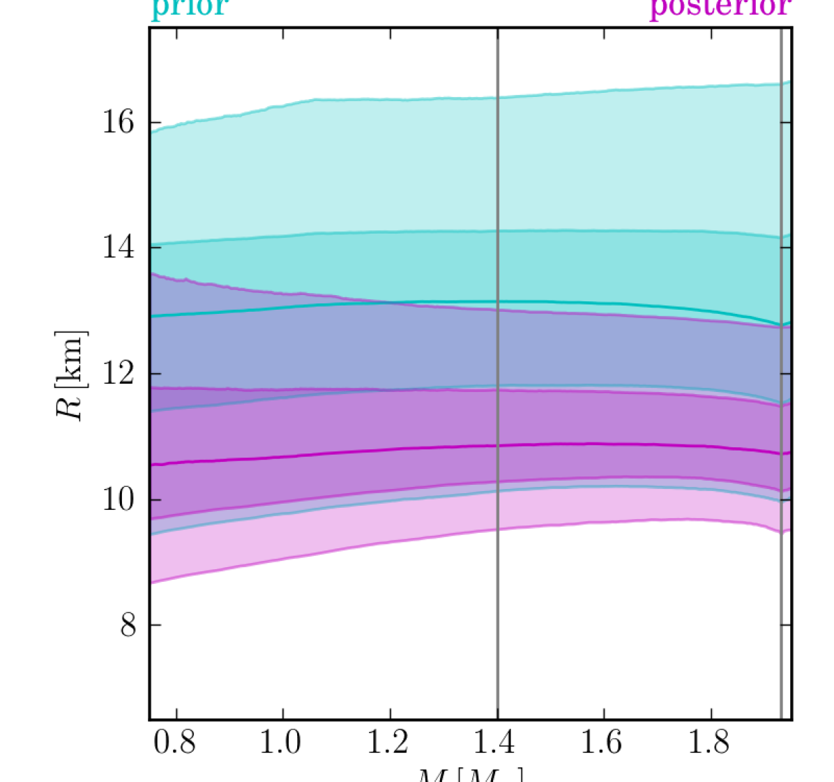
Our posterior process for the EOS immediately yields a posterior distribution for the maximum mass of a nonrotating NS ($M_{\mathrm{max}}$, sometimes called $M_{\mathrm{TOV}}$). Like LE, we find smaller $M_{\mathrm{max}}$ are preferred a posteriori, and that the shift is larger from prior to posterior for the agnostic result. This is consistent with the preference for softer EOSs, many of which struggle to support the 1.93$\,M_{\odot}$ stars required a priori and therefore reach their $M_{\mathrm{max}}$ soon thereafter. We find $M_{\mathrm{max}}=2.064^{+0.260}_{-0.134}$ ($2.017^{+0.238}_{-0.087}$) $M_{\odot}$ with the agnostic (informed) prior, broadly consistent with other constraints in the literature from both GW and EM data (e.g., Refs. Radice et al. (2018); Radice and Dai (2019); Margalit and Metzger (2017); Coughlin et al. (2018)).

Such constraints may be put to the test as more NSs  with large masses are discovered Cromartie et al. (2019). They could play an important role in the analysis of $\mathrm{BHNS}$ systems for which $\tilde{\Lambda}\sim(M_{2}/M_{1})^{4}\Lambda_{2}$ can be quite small. Indeed, precise knowledge of $M_{\mathrm{max}}$ may be the best way to rule out the possibility that the lighter component is a NS, particularly if the source is distant enough that electromagnetic counterparts are unlikely to be detectable. It is worth noting that, while our agnostic posterior favors softer EOSs in the density regime relevant for GW170817, it produces looser $M_{\mathrm{max}}$ constraints than the informed posterior, supporting larger $M_{\mathrm{max}}$ than are allowed by the informed prior. This is associated with the additional model freedom within the agnostic prior, which allows the EOSs to vary significantly at densities larger than those occurring within GW170817’s components.

Table 4 also reports the baryonic mass $M_{b,1.4}$ of a canonical $1.4\,M_{\odot}$ NS. Besides its possible relevance for the amount of matter available to power electromagnetic counterparts, the difference between $M_{b}$ and the NS mass defines the star’s binding energy, with more compact stars corresponding to larger $M_{b}$ at fixed $M$. GW170817 suggests that canonical NSs typically have binding energies of 0.15–0.2$\,M_{\odot}$, corresponding to $>10\%$ of the rest mass of their baryonic content.

IV.2.2 Mass-tidal deformability, mass-radius, and mass-moment of inertia relations

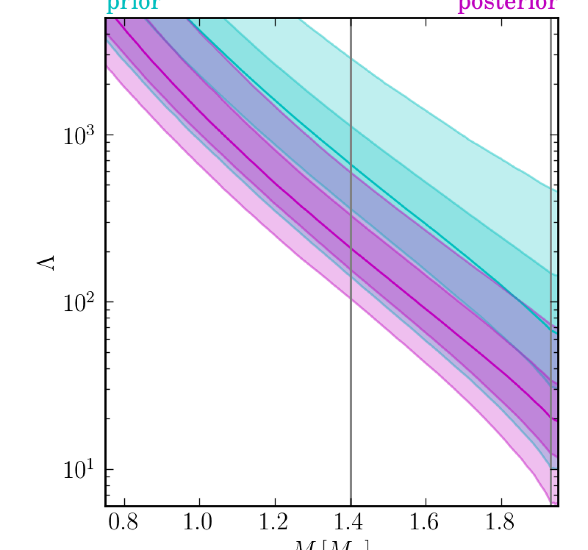
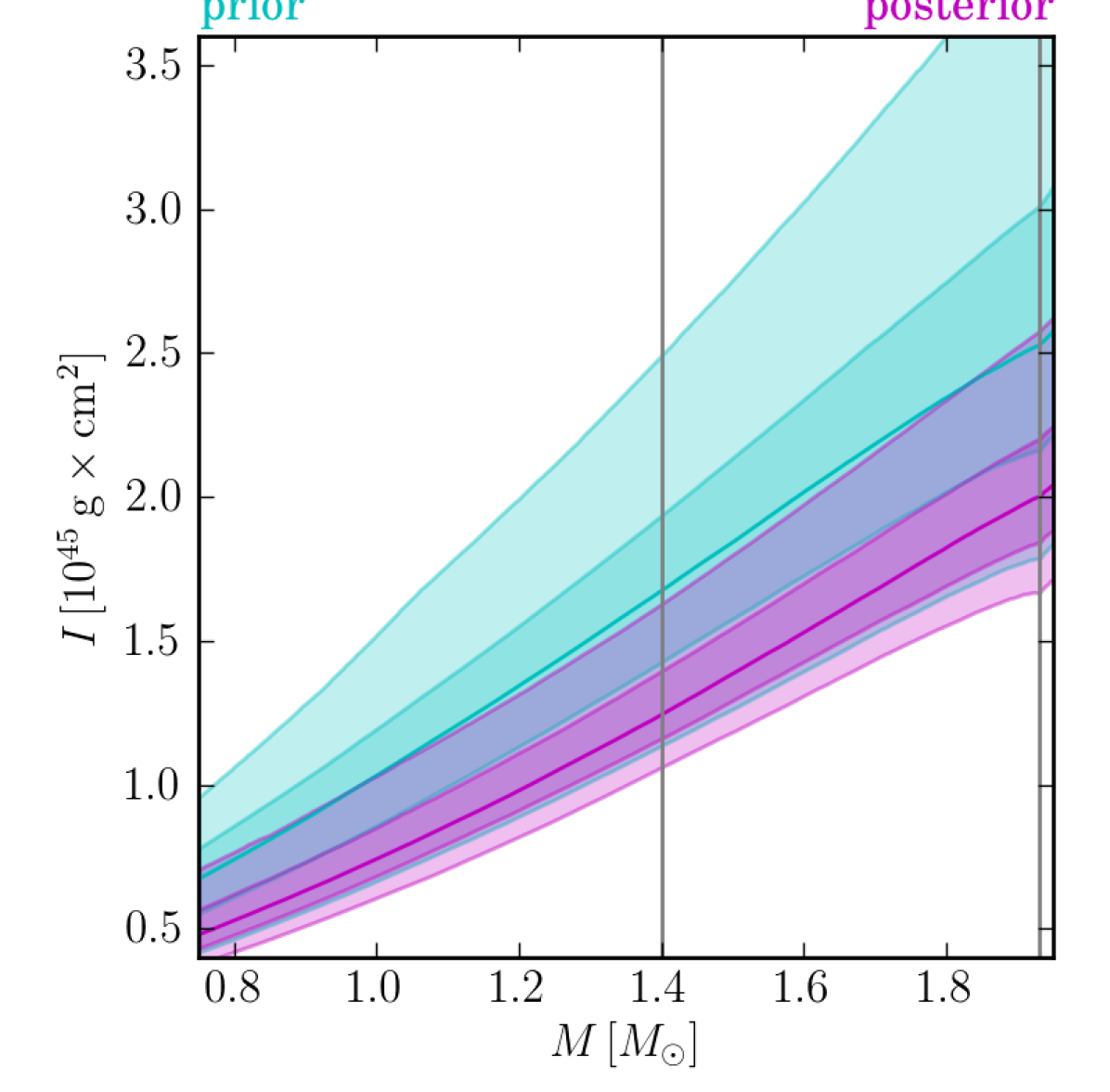
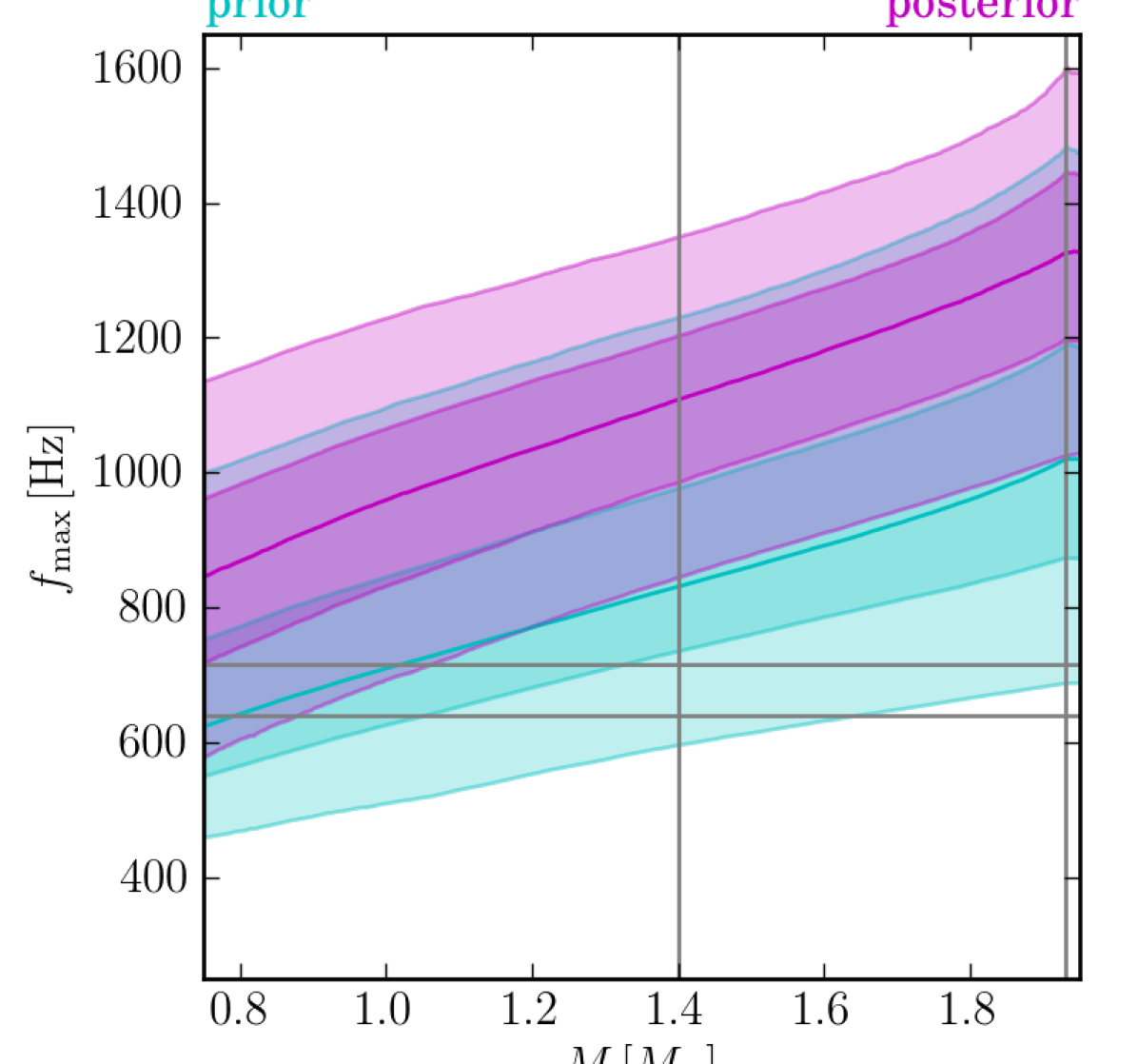
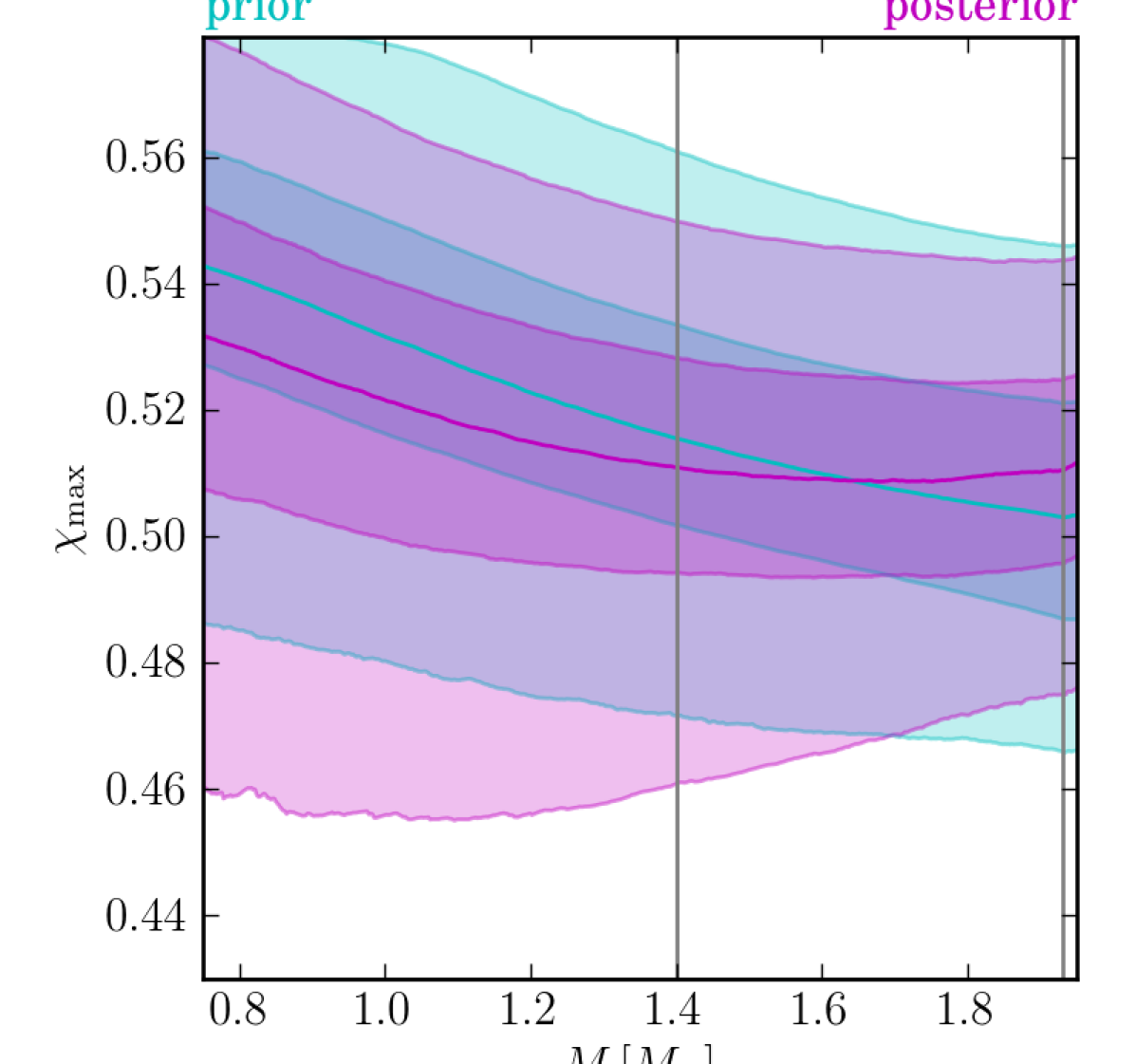
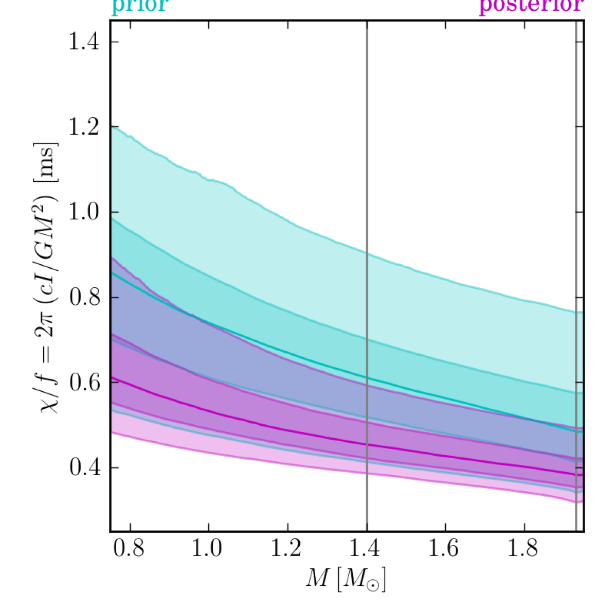
Figure 4 shows our posterior processes for several macroscopic observables as a function of the NS mass. We generally find an a posteriori preference for smaller $\Lambda$, $R$, and $I$ at a given $M$, consistent with relatively compact NSs. This preference is stronger with the agnostic posterior than the informed, again reflecting the agnostic result’s preference for particularly soft EOSs. Table 4 quotes credible regions for a canonical $1.4\,M_{\odot}$ NS, showing good agreement with values reported elsewhere. LE bounded $\Lambda_{1.4}$ to lie between 47 and 608 (384 and 719) at 90% confidence whith their agnostic (informed) prior while Ref. Abbott and et al. (2018) found $\Lambda_{1.4}=190^{+390}_{-120}$. We find $\Lambda_{1.4}=211^{+312}_{-137}$ ($491^{+216}_{-181}$).

Ref. Capano et al. (2019) recently claimed $R_{1.4}=11.0^{+0.9}_{-0.6}$ km based on GW170817 with a strongly theory-informed prior and a parameterization of the sound-speed at high densities Tews et al. (2018a, b). We note that their point-estimate is slightly larger than our agnostic result ($10.86^{+2.04}_{-1.42}\,$km), but that their uncertainties are similar to our informed prior. Their result, then, is likely dependent on their a priori assumptions about the EOS, much like how our informed prior strongly influences the posterior constraints.

The derived relations as functions of mass, informed by GW170817, are likely to be of greatest relevance for future observations of both GW events and electromagnetic sources. For example, X-ray timing of pulsars is expected to constrain their masses and radii Gendreau et al. (2012), radio observations of binary pulsars may measure NSs’ moments of inertia Dewdney et al. (2009); Landry and Kumar (2018); Kumar and Landry (2019), and additional GW observations of coalescing binary NSs should produce $M$–$\Lambda$ measurements consistent with the current constraints Lackey and Wade (2015); Del Pozzo et al. (2013); Agathos et al. (2015). These measurements will effectively act as a null-test of the hypothesis that all NSs share a single EOS, which is currently difficult to constrain with GW170817 alone (see Ref. Abbott and et al. (2019a) and errata of Ref. De et al. (2018)). Indeed, the extreme model freedom allowed by nonparametric analyses will enable novel consistency tests and alternative hypotheses to compare against the universal-EOS assumption.

IV.3 Maximum spin and asteroseismology

The EOS constraints derived from GW170817 have implications for the maximum NS spin, since the Keplerian breakup frequency $f_{\mathrm{dyn}}=\sqrt{GM/R^{3}}/2\pi$ is sensitive to the radius. Numerical relativity simulations of rapidly rotating NSs show that the maximum spin is typically $f_{\mathrm{max}}\sim 0.58f_{\mathrm{dyn}}$, accurate to $\sim 7\%$, after accounting for spin-induced oblateness Cook et al. (1994); Haensel et al. (1995); Stergioulas (2003); Lattimer and Prakash (2004). Here we report estimates for $f_{\mathrm{max}}$, and the corresponding maximum dimensionless spin $\chi_{\mathrm{max}}=cI(2\pi f_{\mathrm{max}})/GM^{2}$, as a function of mass. We note that our calculation for $I$ assumes slowly rotating stars. Oblate, rapidly rotating stars will have larger $I$, and therefore our $\chi_{\mathrm{max}}$ should be interpreted as a lower limit. Previous studies Chakrabarty et al. (2003); Chakrabarty (2005) noted that the maximum spin obtainable for any NS mass is significantly larger than the maximum observed spin frequency, currently $716\,\mathrm{Hz}$ Hessels et al. (2006). We find consistent results, with $\max_{M}\{f_{\mathrm{max}}\}\gtrsim 1.4\,\mathrm{kHz}$. However, the maximum spin frequency at a particular mass can be significantly lower, perhaps by as much as a factor of two. What’s more, the proximity of our lower bound on $f_{\mathrm{max}}$to the observed 716-Hz spin frequency for J1748–2446ad Hessels et al. (2006) may call into question the need for additional braking mechanisms Bildsten (1998); Cutler (2002); Andersson et al. (1999); Levin and Ushomirsky (2001) to limit the spin frequency of recycled millisecond pulsars.

Table 5: Inferred dimensionless spins for several pulsars with known masses with our agnostic (informed) composition-marginalized priors. The upper limits for J0737$-$3039A, in particular, support the low-spin priors assumed in this work and Refs. B. P. Abbott et al. (2017) (LIGO Scientific Collaboration and Virgo Collaboration); Abbott and et al. (2019a, 2018); The LIGO Scientific Collaboration and et al. (2019); Landry and Essick (2019).

PSR	$M\,[M_{\odot}]$	$f\,[\mathrm{Hz}]$	$\chi$
			agnostic	informed
J1807–2500B Lynch et al. (2012)	1.37	238.88	$0.1101^{+0.0317}_{-0.0187}$	$0.1319^{+0.0100}_{-0.0118}$
J0737–3039A Lyne et al. (2004)	1.34	44.05	$0.0205^{+0.0059}_{-0.0036}$	$0.0246^{+0.0019}_{-0.0022}$
J0348+0432 Antoniadis et al. (2013)	2.01	25.56	$0.0098^{+0.0023}_{-0.0017}$	$0.0107^{+0.0011}_{-0.0010}$

The corresponding constraints on the maximum dimensionless spin ($\chi_{\mathrm{max}}$) demonstrate that NS spins must be $\lesssim 0.5$ for astrophysically plausible masses. This provides a natural upper bound on the NS spin prior for future Bayesian analyses if the observed distribution of spins in galactic binaries is not applicable to the broader population. Figure 4 also shows $\chi/f\equiv 2\pi cI/GM^{2}$ as a function of mass, from which we can compute the dimensionless spin of any pulsar given its observed rotation frequency, even if its mass is not precisely known, with the same caveats as $\chi_{\mathrm{max}}$ about rapid rotation. We do this for several pulsars with well-measured masses in Table 5. In particular, the low-spin priors assumed in our work, as well as in Refs. B. P. Abbott et al. (2017) (LIGO Scientific Collaboration and Virgo Collaboration); Abbott and et al. (2019a, 2018); The LIGO Scientific Collaboration and et al. (2019), are motivated by J0737$-$3039A and J1946+2052, with claims that their spins at merger would be below 0.04 and 0.05 Abbott and et al. (2019a), respectively. Our results, which assume $\chi\leq 0.05$ a priori, support this, with J0737–3039A’s current spin inferred to be $0.021^{+0.006}_{-0.004}$ ($0.025^{+0.002}_{-0.002}$) with our agnostic (informed) priors. This is consistent with the dimensionless spin of $\chi\leq 0.034$ inferred for J0737–3039A via universal relations in Ref. Landry and Kumar (2018) without the low-spin assumption.

Similarly, we also find the spin of J1807–2500B ($f=238\,\mathrm{Hz}$ Lynch et al. (2012)), one of the fastest pulsars with a well-measured mass, to be $0.11^{+0.03}_{-0.02}$ ($0.13^{+0.01}_{-0.01}$). Although the dimensionless spin of the fastest known pulsar (J1748–2446ad) depends on its unknown mass, we find $0.25\leq\chi\leq 0.65$ for a wide, astrophysically plausible mass range. In fact, J1748–2446ad’s spin frequency is consistent with $f\gtrsim f_{\mathrm{max}}/2$ at 90% confidence, regardless of mass, and is consistent with $f=f_{\mathrm{max}}$ at $>90\%$ confidence with our agnostic prior if $M\lesssim 1.05\,M_{\odot}$.

Although beyond the scope of the current work, we also note that precise knowledge of the EOS determines the behavior of several dynamical tidal effects. The EOS determines the eigenmode spectra within a NS, and therefore our posterior processes could be used to determine the exact placement and impact of linear resonant dynamical tidal effects due to $f$-modes and low-order $g$-modes during GW-driven inspirals (e.g., Refs. Lai (1994); Yu and Weinberg (2017a, b); Xu and Lai (2017)). Similarly, knowledge of the $r$-mode spectra could inform the CFS instabilities relevant for millisecond pulsars Arras et al. (2003); Chakrabarty et al. (2003); Arras (2005), and knowledge of the $p$- and $g$-mode spectra could improve models of non-linear, non-resonant secular fluid instabilities relevant during the GW inspiral Weinberg et al. (2013); Venumadhav et al. (2014); Weinberg (2016); Essick et al. (2016); Abbott and et al. (2019b). The precise impact of these last two phenomena, however, also depends strongly on the instabilities’ saturation, which themselves are highly uncertain and may prevent precise EOS constraints from making strong predictions about their impact on GW signals.

V Implications for neutron-star composition

Finally, we turn to GW170817’s implications for NS composition. Unlike previous sections, here we break down our agnostic and informed priors according to the composition of the EOSs upon which they were conditioned, presenting results separately for hadronic, hyperonic and quark GPs. More results for each composition are available in Appendix D.

To begin, we compare the evidence for each composition assuming both components were slowly spinning NSs. Table 6 shows the posterior probabilities assuming equal prior odds. Notably, we find weak, but suggestive, evidence in favor of quark matter within NSs with the informed prior, although the agnostic prior prefers EOSs containing only hadrons by a similar amount. The relevance of hadronic vs. quark composition is less clear in the agnostic priors by design, though, as they resemble the input EOSs less closely. This is likely just a statement that the tabulated EOS from the literature containing quark matter are softer, on average, than those labeled either hadronic or hyperonic. It is also worth repeating that none of the compositions are overwhelmingly favored. Nonetheless, the preference for quark EOSs is tantalizing, as theoretical considerations suggest there should be a phase transition to quark matter at sufficiently high densities Baym et al. (2018).

Regardless of the precise details of NS composition, another interesting question is whether there are strong first-order phase transitions within the EOS, leading to, e.g., distinct hadronic and quark phases of matter. One possible signature of such strong phase transitions is the existence of a disconnected hybrid star branch in the $M$-$R$ relation. Stable sequences of NSs exist between critical points in the $M$-$R$ relation; the first stable sequence is called the NS branch, and any subsequent branches at densities above the phase-transition onset are called hybrid star branches (see, e.g., Ref. Schertler et al. (2000)). Although the presence of only a single stable branch does not preclude the existence of phase transitions, multiple stable branches in the $M$-$R$ relation constitute support for a strong first-order phase transition in the EOS. We compute Bayes factors comparing the evidence for EOSs that support multiple stable branches at central densities above $0.8\rho_{\mathrm{nuc}}$ to those with only a single stable branch above $0.8\rho_{\mathrm{nuc}}$ ($B^{n>1}_{n=1}$), finding weak evidence that favors multiple stable branches by a factor of $2$ with our agnostic priors compared to the preference with pulsar data alone. Table 6 shows the results for composition-marginalized priors, and the evidence ratios for each composition separately are of the same order of magnitude. This is far from conclusive, but is suggestive of new physics within NS cores.

Table 6: Posterior probabilities for each composition assuming both components were slowly rotating NSs and equal prior odds, as well as Bayes factors for the number of stable branches in the mass-radius relation with the composition-marginalized priors. Monte-Carlo sampling uncertainties are approximately two orders of magnitude smaller than the point estimates. The Bayes factor for the informed prior is unresolved because its standard deviation is much larger than the point-estimate.

Prior ($\mathcal{H}_{i}$)	$P(\mathrm{Hadronic}|\mathrm{data})$	$P(\mathrm{Hyperonic}|\mathrm{data})$	$P(\mathrm{Quark}|\mathrm{data})$	$B^{n>1}_{n=1}|\textrm{Marginalized}$
informed	$28\%$	$16\%$	$56\%$	unresolved
agnostic	$50\%$	$14\%$	$36\%$	$2.0513\pm(9.5\times 10^{-3})$

Pursuing this further, Figure 5 shows our agnostic prior and posterior processes conditioned on the number of stable branches above $0.8\rho_{\mathrm{nuc}}$. From this we see that, assuming the EOS supports at least one disconnected hybrid branch, GW170817 noticeably prefers EOSs that dramatically soften near $\rho_{\mathrm{nuc}}$ before stiffening significantly around $2\rho_{\mathrm{nuc}}$. While we expect this type of behavior within EOSs that have multiple stable branches, our priors do not have any particular preference for the phase transition to occur in this density range. Intriguingly, the central densities inferred for GW170817 (see Table 1) suggest that any exotic particles associated with the putative phase transition around $\rho_{\mathrm{nuc}}$ would have been present within GW170817’s components’ cores before they coalesced. This finding is consistent with Ref. Paschalidis et al. (2018)’s conclusion that tidal deformability constraints from GW170817 cannot rule out the presence of a hybrid star. Figure 3 shows the processes regardless of the number of stable branches and is dominated by EOSs with a single stable branch since these are favored a priori by a factor of $\sim 10$. While we see the same general trend toward softer EOSs, this manifests as a general decrease in pressure at all densities, whereas there is a notable preference for softening and stiffening at specific densities when there are multiple stable branches.

We also note that the posterior preference for multiple stable branches depends on the precise lower limit of $M_{\mathrm{max}}$ allowed in our priors. The requirement that $M_{\mathrm{max}}\geq 1.93\,M_{\odot}$ forces the EOS to become stiff at high densities, thereby imparting the preference for EOSs that stiffen again after they initially soften. Without that requirement, EOSs that do not stiffen significantly (and hence support only a single stable branch) can still reproduce the GW170817 data reasonably well, weakening the modest preference for EOSs with multiple stable branches. We expect observations of more massive pulsars (e.g., Cromartie et al. (2019)) to increase the preference for multiple stable branches, all else being equal.

While we stress that the statistical evidence in favor of EOSs that support multiple stable branches in the $M$-$R$ relation is weak, GW170817’s preference for soft EOSs, in conjunction with the existence of a 2 $M_{\odot}$ pulsar, could be interpreted as evidence for a strong phase transition between $\rho_{\mathrm{nuc}}$ and 2$\rho_{\mathrm{nuc}}$, although the precise onset density, pressure, and latent energy associated with such a phase transition are still largely uncertain. Nonetheless, some theoretical studies of chiral effective field theory suggest that the purely hadronic model for the EOS will break down in this density range due to phase transitions Tews et al. (2018a, b, 2019); Furnstahl et al. (2015). This coincidence is intriguing, especially since none of our input candidate EOSs are computed within the chiral effective field theory framework. It is therefore possible that we have observed exotic particles in the cores of coalescing NSs with GW170817.

Figure 5: Agnostic EOS prior (cyan) and posterior (magenta) processes for EOSs that support multiple stable branches in the $M$-$R$ relation above $\rho_{c}=0.8\rho_{\mathrm{nuc}}$ after marginalizing over composition. The equivalent processes for EOSs that support a single stable branch are indistinguishable from Figure 3. The general preference for softer EOSs a posteriori manifests as a dramatic softening at or below $\rho_{\mathrm{nuc}}$ before stiffening at approximately 2$\rho_{\mathrm{nuc}}$. Gray lines denote $\rho_{\mathrm{nuc}}$, 2$\rho_{\mathrm{nuc}}$, and 6$\rho_{\mathrm{nuc}}$, respectively. Bayes factors between multiple and single stable branches for the agnostic priors are $B^{n>1}_{n=1}=2.0513\pm(9.5\times 10^{-3})$, $1.5274\pm(6.8\times 10^{-3})$, $4.084\pm(1.9\times 10^{-2})$, and $1.684\pm(1.7\times 10^{-2})$ for the marginalized, hadronic, hyperonic, and quark compositions, respectively.

VI Discussion

We present a comprehensive nonparametric inference of the equation of state of neutron star matter, as informed by GW170817. Nonparametric analyses allow for expansive model freedom, thereby mitigating the kind of systematic errors associated with parameterized EOSs while additionally providing transparent priors on physical quantities. Our nonparametric approach does not assign any particular importance to specific densities or pressures a priori, and the features observed in the inferred EOS a posteriori are therefore driven by the data rather than prior beliefs. We improve the nonparametric priors introduced in Landry & Essick Landry and Essick (2019) by including additional tabulated EOSs from the literature and constructing separate priors for different underlying compositions. We analyze publicly available data from GW170817 LIGO Scientific Collaboration and Virgo Collaboration after conditioning on the existence of massive pulsars Antoniadis et al. (2013); Cromartie et al. (2019) and find that GW170817 favors soft EOSs, with $p(2\rho_{\mathrm{nuc}})=1.81^{+2.80}_{-1.80}\times 10^{34}$ ($4.44^{+1.09}_{-1.34}\times 10^{34}$) dyn/cm² and $p(6\rho_{\mathrm{nuc}})=8.56^{+4.81}_{-3.88}\times 10^{35}$ ($6.84^{+5.58}_{-1.12}\times 10^{35}$) dyn/cm², in agreement with previous studies Abbott and et al. (2018); Landry and Essick (2019). Given these constraints on the EOS, we are able to infer properties of a canonical $1.4\,M_{\odot}$ neutron star. In particular, we find a posteriori medians and 90% highest-probability-density credible regions of $\Lambda_{1.4}=211^{+312}_{-137}$ ($491^{+216}_{-181}$), $R_{1.4}=10.86^{+2.04}_{-1.42}$ ($12.51^{+1.00}_{-0.88}$) km, and a maximum mass $M_{\mathrm{max}}=2.064^{+0.260}_{-0.134}$ ($2.017^{+0.238}_{-0.087}$) $M_{\odot}$ with our model-agnostic (model-informed) priors marginalized over composition. We find mild evidence against a $\mathrm{BBH}$ progenitor, with $B^{\rm NS}_{\mathrm{BBH}}=3.3\pm 1.4$, in accordance with analyses of individual tabulated EOSs The LIGO Scientific Collaboration and et al. (2019) and the observation of electromagnetic counterparts Abbott and et al. (2017a, b). Intriguingly, and for the first time, we find a weak preference for EOS containing quark matter with our informed prior. We also find a preference for EOSs that support multiple stable branches in their $M$–$R$ and $M$–$\Lambda$ relations with our agnostic prior when comparing results using GW and pulsar data against pulsar data alone. While far from conclusive, we note that if the EOS supports multiple stable branches, there is a noticeable preference for dramatic softening around $\rho_{\mathrm{nuc}}$ followed by stiffening around 2$\rho_{\mathrm{nuc}}$, consistent with a phase transition and predictions for where chiral effective field theory may break down Tews et al. (2018a, b, 2019); Furnstahl et al. (2015). However, the exact onset density, pressure, and latent energy remain uncertain by at least a factor of a few. We emphasize that these results are informed solely by GW170817 data and massive pulsar observations; our nonparametric prior processes were not constructed with any particular importance given to these densities, or to EOSs with particular phase transitions.

Using our posterior processes, we estimate the amount of baryonic mass dynamically ejected during the coalescence ($M_{\mathrm{ejecta}}^{(\mathrm{dyn})}=6.5^{+6.3}_{-3.9}\times 10^{-3}\,M_{\odot}$) and its velocity ($v_{\mathrm{ejecta}}^{(\mathrm{dyn})}/c=0.257^{+0.027}_{-0.034}$), concluding that it must have been a subdominant component of the total ejected mass that powered the associated kilonova ($\gtrsim 0.05\,M_{\odot}$ Coughlin et al. (2018)).

We also point out that the lower limit on the maximum spin frequency of NSs can approach the observed spin frequencies of some millisecond pulsars if they have relatively low masses ($\lesssim M_{\odot}$). Because the masses of many millisecond pulsars are unknown, this may warrant a reexamination of the need for additional braking mechanisms, such as $r$-mode CFS instabilities. Indeed, although the fastest-spinning known pulsar does not have a precise mass measurement, we find its observed spin is $\gtrsim f_{\mathrm{max}}/2$ for all astrophysically plausible masses at 90% confidence, and that it is consistent with $f=f_{\mathrm{max}}$ at $>90\%$ confidence if it is lighter than $M_{\odot}$.

While our results already extend beyond previous studies, there are several ways our analysis might be further improved. For example, one could incorporate an improved representation of the GW likelihood, perhaps through a KDE with better control over systematics associated with hard prior bounds, or explicitly account for uncertainty in the likelihood model due to the finite number of posterior samples available. However, it is believed that systematic uncertainties from such issues are currently dominated by statistical uncertainties. Similarly, improved covariance kernels within our GPs could allow for even more model freedom beyond the already formidable range allowed by our mixture model over different hyperparameters. In particular, kernels that support different length scales at different pressures, to further enhance our ability to model different levels of theoretical uncertainty at different pressures, could be promising. Even with more complicated kernels, our hyperparameters will retain immediately interpretable meanings, such as how quickly the energy density can change with pressure.

Beyond these technical improvements, one could incorporate information from other observations in a more sophisticated way. For example, instead of simply discarding any synthetic EOSs that do not support a $1.93\,M_{\odot}$ star based on the approximate 2-$\sigma$ lower limit from J0348+0432 Antoniadis et al. (2013) and J0740+6620 Cromartie et al. (2019), we could instead use the entire uncertainty in such mass measurements to weight each EOS, similar to what is proposed in Ref. Miller et al. (2019). These weights can be combined with likelihoods from other GW observations as well as $M$–$R$ measurements from X-ray timing Gendreau et al. (2012), moment-of-inertia measurements from radio observations Dewdney et al. (2009); Landry and Kumar (2018), or even mass and frequency measurements from millisecond pulsars in a single self-consistent framework without the need for hard thresholds. We will explore this avenue in future work.

Similarly, including better constraints on the theoretical uncertainty at low densities by matching to chiral effective field theory with theoretical uncertainties from truncating series expansions Tews et al. (2018a, b, 2019); Furnstahl et al. (2015) should further constrain our priors. We note, though, that GW170817 produces posterior processes that already tend to follow the prior relatively closely below $\rho_{\mathrm{nuc}}$ (see Figure 5). Along the same lines, forcing our synthetic EOSs to asymptote to $c_{s}^{2}\rightarrow c^{2}/3$ at high density, consistent with ultra-relativistic matter, may prove interesting.

Nonetheless, our nonparametric inference already provides novel results. Because of the extreme model freedom supported in our prior processes, we see tantalizing hints of new physics and phase transitions within the cores of NSs. In particular, the suggestive preference for quark matter and EOSs that support multiple stable branches by factors of $\approx 2$ imply the possible presence of a phase transition between $\rho_{\mathrm{nuc}}$ and 2$\rho_{\mathrm{nuc}}$ with no special significance given to these densities a priori. While the statistical evidence remains marginal at best, the agreement between these observations and predictions from theory could be taken as evidence that we have already seen new states of matter within NS cores. Indeed, this demonstrates the key role GWs will play in determining the supranuclear EOS and the unique capabilities of nonparametric analyses.

In the near future, our nonparametric analyses will allow for further investigations into possible phase transitions in supranuclear matter, including the maximum sound-speed achieved within NSs. They provide for natural null tests of the universal-EOS hypothesis, but also allow for natural alternative hypotheses by spanning the space of EOSs allowed by causality and thermodynamic stability regardless of their underlying composition. Finally, our analysis can naturally incorporate information from arbitrarily many sources, including constraints about high-density matter from the observation of massive pulsars and information about nuclear densities from coalescing NSs via GWs and accreting systems through X-ray timing, while self-consistently accounting for selection effects, astrophysical populations, and formation channels. As demonstrated by our novel results, nonparametric analyses provide the best chance to capture new physics without systematic modeling errors using multi-messenger astrophysical observations and will only become more important in the years to come.

Appendix A Details of nonparametric prior construction

While Section II provides an overview of how we construct our priors, we report many important technical details here. First, as in LE, each tabulated $\varepsilon(p)$ is resampled to obtain a process for $\phi(p)$ using $K_{\mathrm{se}}$ and $K_{\mathrm{wn}}$ with hyperparameters optimized separately for each EOS. Because the data for each tabulated EOS represents a single function, we optimize hyperparameters using the marginal likelihood (see Section 5.4.1 of Rasmussen and Williams (2006))

$$\log P_{\mathrm{ML}}(\varepsilon|p,\vec{\sigma})=-\frac{1}{2}(\varepsilon_{i}-\mu_{i})\left(K^{-1}\right)_{ij}(\varepsilon_{j}-\mu_{j})\\ -\frac{N}{2}\log\left(2\pi\right)-\frac{1}{2}\log\left|K_{ij}\right|$$ (16)

where $N$ is the dimensionality of $\varepsilon_{i}$ and $|K_{ij}|$ is the determinant of the covariance matrix. This likelihood, which is the probability of obtaining the observed data given a GP with the specified hyperparameters, selects the best-fit element of the statistical model defined by our GP. We typically observe strong correlations between $\sigma$ and $l$, as increasing either increases the correlation between neighboring points.

We note that EOSs with sharp features, like strong first-order phase transitions, are somewhat difficult to model with a squared-exponential kernel because $K_{\mathrm{se}}$ strictly generates analytic functions. Nonetheless, we find it is still possible to adequately represent the behavior seen in, e.g., tabulated EOSs that contain quark matter over the densities relevant for GW170817.

We then construct separate GPs to represent all tabulated EOSs belonging to the same composition and family using $K_{\mathrm{se}}$, $K_{\mathrm{wn}}$, and $K_{\mathrm{mv}}$. Because these GPs are meant to emulate the typical behavior of a group of proposed EOSs rather than reproduce a single function, we select hyperparameters based on a cross-validation likelihood (see Section 5.4.2 of Rasmussen and Williams (2006) and Eq. (10)). The cross-validation likelihood selects hyperparameters that produce synthetic EOSs with a variance similar to what is seen between elements of the training set. We select a single set of optimal hyperparameters based on the cross-validation likelihood separately for each composition and family.

Similar to $P_{\mathrm{ML}}$, $P_{\mathrm{CV}}$ shows strong correlations between $\sigma$ and $l$. These are often independent of $\sigma_{\mathrm{obs}}$ and $m$, which themselves show strong degeneracies. Usually, the input EOSs strongly prefer a specific ($\sigma$, $l$) pair, indicative of the typical correlations and length scales in the underlying data. Additionally, the cross-validation requires at least some spread in the conditioned processes, meaning that as long as either $\sigma_{\mathrm{obs}}$ or $m$ is sufficiently large, there is little preference for the precise combination.

After obtaining GPs for each composition and family combination, we construct agnostic and informed GPs for each composition, both of which are conditioned on the GPs for all families within that composition. Each family is equally weighted so that those containing many slightly different tabulated EOSs are not more strongly weighted than families with fewer EOSs, as the number of tabulated EOSs in each family may depend on different authors’ propensities to publish. We note that this is not a unique choice and different relative weights would produce different priors.

As described in Section II.1, we again use the cross-validation likelihood (Eq 10) with $K_{\mathrm{se}}$, $K_{\mathrm{wn}}$, and $K_{\mathrm{mv}}$ to obtain processes that emulate the behavior seen within each composition, observing similar correlations to those observed within each combination of composition and family. However, instead of selecting a single set of hyperparameters, we sample from $P_{\mathrm{CV}}$ as in Eq. 11. This generates a mixture model of many different GPs from which we sample when drawing from our priors.

We generate informed priors via simulated annealing, repeatedly Monte-Carlo sampling from the hyperprior as we slowly decrease the temperature in order to find the high-likelihood portions of hyperparameter space. However, we note that taking the limit $T\rightarrow\infty$ with arbitrary prior bounds may not produce the range of variability desired for the agnostic prior. Specifically, we identify several regions of hyperparameter space that produce nearly identical conditioned processes, several of which we consider “too tight” as they do not produce a broad range of synthetic EOSs. Therefore, we impose several additional hyperprior constraints for the agnostic priors. We require $\sigma\geq 1$, $\sigma_{\mathrm{obs}}\geq 1$, $m\geq 1$, and $(\sigma_{\mathrm{obs}}^{2}+m^{2})\geq 2\sigma^{2}$. The first condition allows the resulting processes to deviate significantly from the mean, while the second and third conditions make the conditioned process less sensitive to the specific behavior seen in the tabulated EOSs. The final condition on the ratio of hyperparameters avoids situations where the modeling uncertainty ($\sigma_{\mathrm{obs}}$, $m$) is significantly smaller than the marginal $K_{\mathrm{se}}$ uncertainty ($\sigma$). When that happens, the conditioned process returns a weighted average of the input EOSs with a variance similar to the modeling uncertainty rather than $\sigma$, as would be expected when taking the average of many independent Gaussian-distributed variates. In the opposite extreme, where the modeling uncertainty is much larger than $\sigma$, the resulting conditioned process follows the prior mean with variances characteristic of $\sigma$, which produce reasonably broad synthetic EOSs because we require $\sigma\geq 1$. We additionally allow $l$ to vary over nearly an order of magnitude.

Appendix B Optimal Gaussian kernel density estimate representations of the gravitational-wave likelihood

Our Gaussian KDE model for the GW likelihood is constructed in the four-dimensional space spanned by $M_{1}$, $M_{2}$, $\Lambda_{1}$, and $\Lambda_{2}$. We assume a diagonal covariance ($C_{ij}$) within our Gaussian kernels, optimizing the bandwidths directly by varying a scale parameter for each dimension’s sample variance so that

$$C_{ij}=b^{2}\sigma_{i}^{2}\delta_{ij}\quad\left|\quad\sigma^{2}_{i}=\frac{1}{N}\sum\limits_{\alpha}\left(x^{(\alpha)}_{i}\right)^{2}-\left(\frac{1}{N}\sum\limits_{\alpha}x^{(\alpha)}_{i}\right)^{2}\right.$$ (17)

Pragmatically, this is done by whitening the samples with the sample variance in each dimension separately and then optimizing a scale parameter for a covariance proportional to the identity matrix. This is achieved by directly maximizing a leave-one-out cross-validation likelihood as a function of the scale parameter $b$

$$\log L_{\mathrm{CV}}=\sum\limits_{i}^{N}\log\left(\frac{1}{N-1}\sum\limits_{j\neq i}^{N-1}k(x_{i},x_{j};b)\right)$$ (18)

where $k$ is our multi-dimensional Gaussian kernel. Using the available samples LIGO Scientific Collaboration and Virgo Collaboration , we find optimal bandwidths of $b_{\mathrm{opt}}=0.1247$ ($0.0905$) for the low-spin (high-spin) data set.

Furthermore, to account for hard prior bounds like $\Lambda_{1,2}\geq 0$, we reflect our samples across such boundaries, de facto forcing the KDE’s derivative to vanish at the boundary in directions perpendicular to the boundary. This can introduce systematic biases beyond those produced by the smoothing inherent in all KDE models. We measure the scale of their impact on Monte-Carlo integrals conducted along the boundary by comparing estimates with and without reflected samples. Note that the relative weight assigned to samples far from the boundary, i.e. most of the $\mathrm{BNS}$ Monte-Carlo points, are virtually unaffected by such issues, and these primarily concern $\mathrm{NSBH}$, $\mathrm{BHNS}$, and $\mathrm{BBH}$ models.

Appendix C Tabulated equations of state used to condition nonparametric priors

Table 7 lists the tabulated candidate EOSs used to condition our nonparametric priors, including their $M_{\mathrm{max}}$ and source references.

Table 7: Tabulated EOSs grouped in the same way we construct our priors, first by combining members of each family of underlying nuclear effective forces separately, and then combining separate families for each composition.

Composition	Family	Moniker	$M_{\mathrm{max}}\ [M_{\odot}]$	Reference
Hadronic	BSK	bsk20	$2.16$	Goriely et al. (2010)
		bsk21	$2.27$
		bsk22	$2.26$	Goriely et al. (2013)
		bsk23	$2.27$
		bsk24	$2.28$
		bsk25	$2.22$
		bsk26	$2.15$
	BSR	bsr2	$2.38$	Agrawal (2010)
		bsr6	$2.43$
	DD	dd2	$2.42$	Banik et al. (2014)
		ddhd	$2.14$	Gaitanos et al. (2004)
		ddme2	$2.48$	Lalazissis et al. (2005)
	ENG	eng	$2.24$	Engvik et al. (1996)
	GM	gm1	$2.36$	Glendenning and Moszkowski (1991)
	KDE	kde0v	$1.96$	Gulminelli and Raduta (2015)
		kde0v1	$1.97$	Agrawal et al. (2005)
	MPA	mpa1	$2.46$	Müther et al. (1987)
	NL	nl3	$2.77$	Lalazissis et al. (1997)
	R	rs	$2.12$	Friedrich and Reinhard (1986)
	SK	sk255	$2.14$	Agrawal et al. (2003)
		sk272	$2.23$
		ski2	$2.16$	Reinhard and Flocard (1995)
		ski3	$2.24$
		ski4	$2.17$
		ski5	$2.24$
		ski6	$2.19$	Nazarewicz et al. (1996)
		skmp	$2.11$	Bennour et al. (1989)
		skop	$1.97$	Reinhard et al. (1999)
	SLY	sly230a	$2.10$	Chabanat et al. (1997)
		sly2	$2.05$	Chabanat (1995)
		sly9	$2.05$
		sly	$2.16$	Douchin and Haensel (2001)
	TM	tm1	$2.18$	Sugahara and Toki (1994)

Composition	Family	Moniker	$M_{\mathrm{max}}\ [M_{\odot}]$	Reference
Hyperonic	BSR	bsr2y	$2.00$	Fortin et al. (2016)
		bsr6y	$2.02$
	DD	dd2y	$2.00$	Fortin et al. (2016)
		ddme2y	$2.09$
	GM	gm1b	$1.99$	Gusakov et al. (2014)
		gm1y	$2.02$	Fortin et al. (2016)
	H	h4	$2.03$	Lackey et al. (2006)
	NL	nl3y	$2.31$	Fortin et al. (2016)
	TM	tm1c	$2.06$	Gusakov et al. (2014)
Quark	ALF	alf2	$2.09$	Alford et al. (2005)
		alf4	$1.94$
	DDQ	ddq0625	$1.93$	Bonanno and Sedrakian (2012)
		ddq0630	$2.07$
		ddq0825	$1.99$
		ddq0830	$2.08$
	HQC	hqc18	$2.05$	Baym et al. (2019)
		hqc19	$2.07$

Appendix D Supplementary figures and tables

We present a few additional tables and figures relevant for our analyses. Tables 8-10 contain results broken down by composition. Fig. 6 shows informed-prior results for functional relations between generic NS observables, and Fig. 7 plots distributions for canonical and maximum-mass quantities.

Table 8: Medians a posteriori and highest-probability-density 90% credible regions for macroscopic observables associated with GW170817, with priors broken down according to the composition of the EOS upon which they were conditioned.

Prior ($\mathcal{H}_{i}$)		$M_{1}\,[M_{\odot}]$	$M_{2}\,[M_{\odot}]$	$\Lambda_{1}$	$\Lambda_{2}$	$\tilde{\Lambda}$	$R_{1}\,[\mathrm{km}]$	$R_{2}\,[\mathrm{km}]$	$\rho_{c,1}\,[10^{14}\,\mathrm{g}/\mathrm{cm}^{3}]$	$\rho_{c,2}\,[10^{14}\,\mathrm{g}/\mathrm{cm}^{3}]$
informed	Hadronic	$1.45^{+0.10}_{-0.09}$	$1.28^{+0.08}_{-0.08}$	$444^{+222}_{-250}$	$961^{+532}_{-382}$	$658^{+188}_{-156}$	$12.96^{+0.57}_{-0.55}$	$13.03^{+0.55}_{-0.57}$	$7.07^{+1.10}_{-0.99}$	$6.41^{+0.77}_{-0.85}$
	Hyperonic	$1.46^{+0.08}_{-0.09}$	$1.28^{+0.08}_{-0.07}$	$502^{+294}_{-187}$	$1114^{+495}_{-414}$	$760^{+131}_{-150}$	$13.20^{+0.39}_{-0.43}$	$13.28^{+0.34}_{-0.45}$	$7.02^{+0.87}_{-0.91}$	$6.19^{+0.71}_{-0.65}$
	Quark	$1.46^{+0.12}_{-0.10}$	$1.27^{+0.08}_{-0.10}$	$315^{+210}_{-179}$	$742^{+425}_{-328}$	$496^{+145}_{-166}$	$12.14^{+0.63}_{-0.68}$	$12.10^{+0.59}_{-0.76}$	$7.83^{+1.44}_{-1.30}$	$6.94^{+1.06}_{-0.94}$
agnostic	Hadronic	$1.50^{+0.13}_{-0.13}$	$1.25^{+0.11}_{-0.10}$	$124^{+181}_{-103}$	$379^{+402}_{-257}$	$216^{+266}_{-141}$	$10.66^{+1.66}_{-1.35}$	$10.59^{+1.79}_{-1.57}$	$10.38^{+3.35}_{-3.76}$	$9.36^{+2.59}_{-3.21}$
	Hyperonic	$1.47^{+0.12}_{-0.11}$	$1.27^{+0.10}_{-0.09}$	$268^{+324}_{-229}$	$690^{+600}_{-522}$	$466^{+337}_{-337}$	$12.14^{+1.39}_{-1.90}$	$12.15^{+1.44}_{-2.07}$	$8.29^{+3.51}_{-2.48}$	$7.32^{+3.11}_{-1.96}$
	Quark	$1.49^{+0.13}_{-0.12}$	$1.25^{+0.10}_{-0.10}$	$162^{+260}_{-135}$	$456^{+483}_{-310}$	$262^{+335}_{-162}$	$10.94^{+1.80}_{-1.27}$	$10.84^{+1.88}_{-1.45}$	$9.46^{+3.02}_{-3.52}$	$8.55^{+2.41}_{-2.90}$

Table 9: Medians a posteriori and highest-probability-density 90% credible regions for a few canonical macroscopic quantities, with priors broken down according to the composition of the EOS upon which they were conditioned.

Prior ($\mathcal{H}_{i}$)		$\Lambda_{1.4}$	$R_{1.4}\,[\mathrm{km}]$	$I_{1.4}\,[10^{45}\,\mathrm{g}\,\mathrm{cm}^{2}]$	$M_{b,1.4}\,[M_{\odot}]$	$M_{\mathrm{max}}\,[M_{\odot}]$
informed	Hadronic	$561^{+163}_{-137}$	$12.98^{+0.55}_{-0.56}$	$1.61^{+0.12}_{-0.11}$	$1.552^{+0.010}_{-0.010}$	$2.233^{+0.098}_{-0.098}$
	Hyperonic	$650^{+113}_{-134}$	$13.23^{+0.37}_{-0.43}$	$1.67^{+0.08}_{-0.10}$	$1.589^{+0.008}_{-0.007}$	$2.017^{+0.071}_{-0.084}$
	Quark	$427^{+125}_{-143}$	$12.14^{+0.59}_{-0.72}$	$1.50^{+0.11}_{-0.14}$	$1.568^{+0.017}_{-0.016}$	$1.978^{+0.082}_{-0.048}$
agnostic	Hadronic	$185^{+228}_{-119}$	$10.65^{+1.69}_{-1.42}$	$1.21^{+0.29}_{-0.21}$	$1.591^{+0.055}_{-0.057}$	$2.091^{+0.272}_{-0.161}$
	Hyperonic	$399^{+296}_{-285}$	$12.15^{+1.37}_{-1.99}$	$1.47^{+0.26}_{-0.34}$	$1.602^{+0.048}_{-0.024}$	$2.038^{+0.225}_{-0.108}$
	Quark	$228^{+291}_{-140}$	$10.91^{+1.83}_{-1.31}$	$1.28^{+0.33}_{-0.20}$	$1.588^{+0.046}_{-0.052}$	$2.042^{+0.242}_{-0.112}$

Table 10: Medians a posteriori and highest-probability-density 90% credible regions for canonical central densities and pressures at reference densities, with priors broken down according to the composition of the EOS upon which they were conditioned.

Prior ($\mathcal{H}_{i}$)		$\rho_{c,1.4}\,[\mathrm{g}/\mathrm{cm}^{3}]$	$p(\rho_{\mathrm{nuc}})\,[\mathrm{dyn}/\mathrm{cm}^{2}]$	$p(2\rho_{\mathrm{nuc}})\,[\mathrm{dyn}/\mathrm{cm}^{2}]$	$p(6\rho_{\mathrm{nuc}})\,[\mathrm{dyn}/\mathrm{cm}^{2}]$
informed	Hadronic	$6.87^{+0.85}_{-0.84}\times 10^{14}$	$6.07^{+1.29}_{-1.29}\times 10^{33}$	$4.71^{+0.96}_{-0.84}\times 10^{34}$	$11.81^{+1.45}_{-1.46}\times 10^{35}$
	Hyperonic	$6.71^{+0.72}_{-0.64}\times 10^{14}$	$5.86^{+1.03}_{-1.01}\times 10^{33}$	$4.84^{+0.59}_{-0.66}\times 10^{34}$	$6.70^{+0.64}_{-0.60}\times 10^{35}$
	Quark	$7.47^{+1.15}_{-1.02}\times 10^{14}$	$3.18^{+1.35}_{-1.24\times 10^{33}}$	$4.06^{+1.14}_{-1.28}\times 10^{34}$	$6.55^{+0.87}_{-0.89}\times 10^{35}$
agnostic	Hadronic	$9.95^{+2.96}_{-3.36}\times 10^{14}$	$2.09^{+4.25}_{-1.97}\times 10^{33}$	$1.54^{+2.21}_{-1.53}\times 10^{34}$	$9.50^{+5.12}_{-3.45}\times 10^{35}$
	Hyperonic	$7.89^{+3.27}_{-2.17}\times 10^{14}$	$4.22^{+2.80}_{-3.71}\times 10^{33}$	$3.34^{+2.09}_{-3.10}\times 10^{34}$	$7.18^{+3.43}_{-2.63}\times 10^{35}$
	Quark	$9.07^{+2.73}_{-3.09}\times 10^{14}$	$1.91^{+3.58}_{-1.78}\times 10^{33}$	$1.87^{+2.87}_{-1.85}\times 10^{34}$	$7.84^{+3.93}_{-3.59}\times 10^{35}$

model-informed

Figure 6: Processes relating a few macroscopic observables after marginalizing over EOS-composition with the informed prior. Prior (cyan) and posterior (magenta) processes for (left) tidal deformability ($\Lambda$; top), radius ($R$; middle), and moment-of-inertia ($I$; bottom) as functions of mass as well as (right) the maximum spin frequency ($f_{\mathrm{max}}$; top), maximum dimensionless spin parameter ($\chi_{\mathrm{max}}$; middle), and $\chi/f$ (bottom). Shaded regions denote the 50% and 90% symmetric credible regions for the marginal distribution of each observable at each mass. Solid lines denote the median and vertical lines denote canonical $1.4\,M_{\odot}$ stars. Horizontal grey lines in the top-right panel denote the measured spin frequencies of J1748–2446ad ($716\,\mathrm{Hz}$ Hessels et al. (2006)) and B1937+241 (641 Hz Backer et al. (1982)), which lie below but near the lower limits for $f_{\mathrm{max}}$.

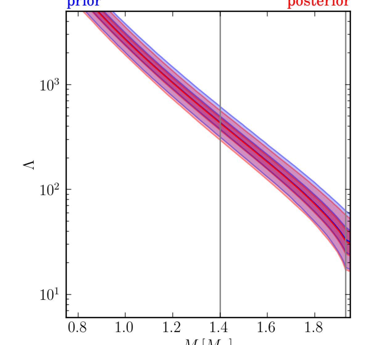
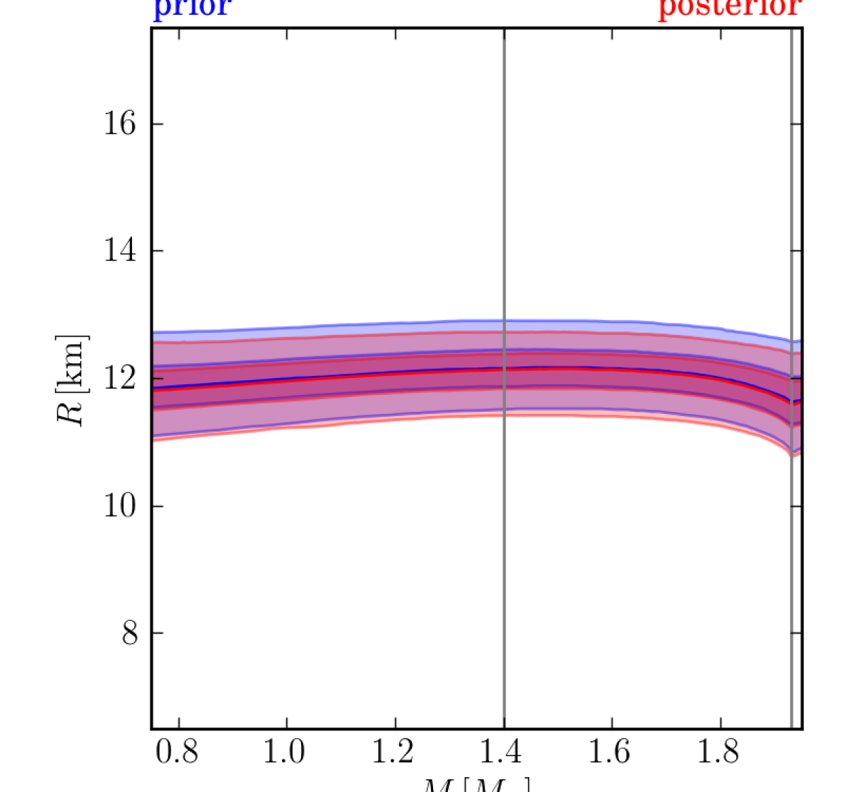
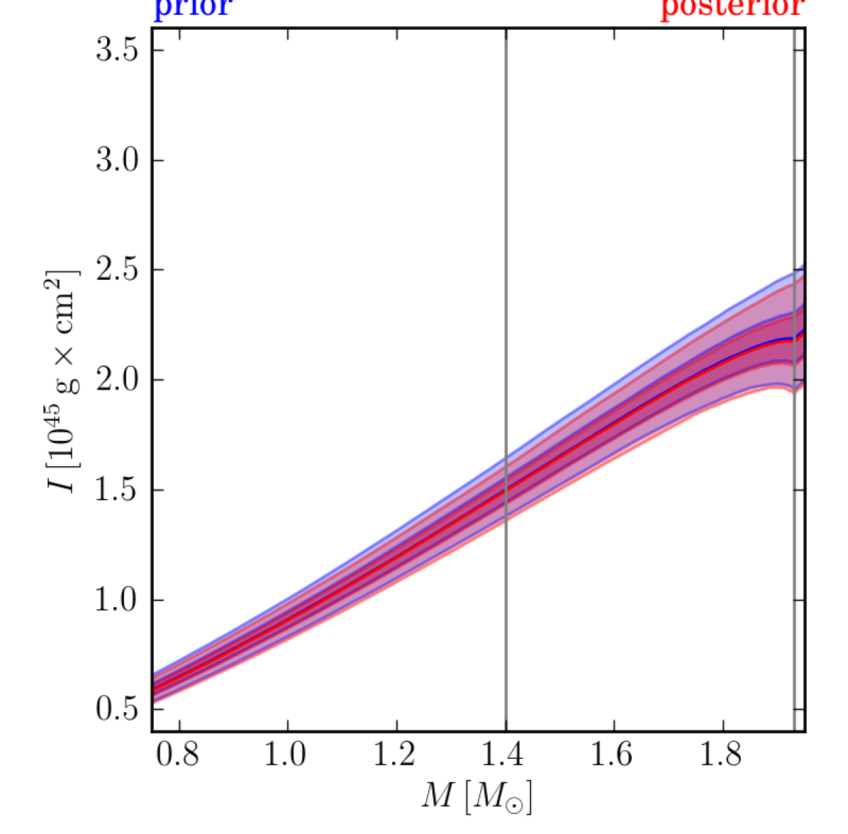
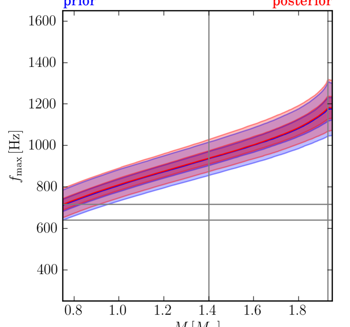
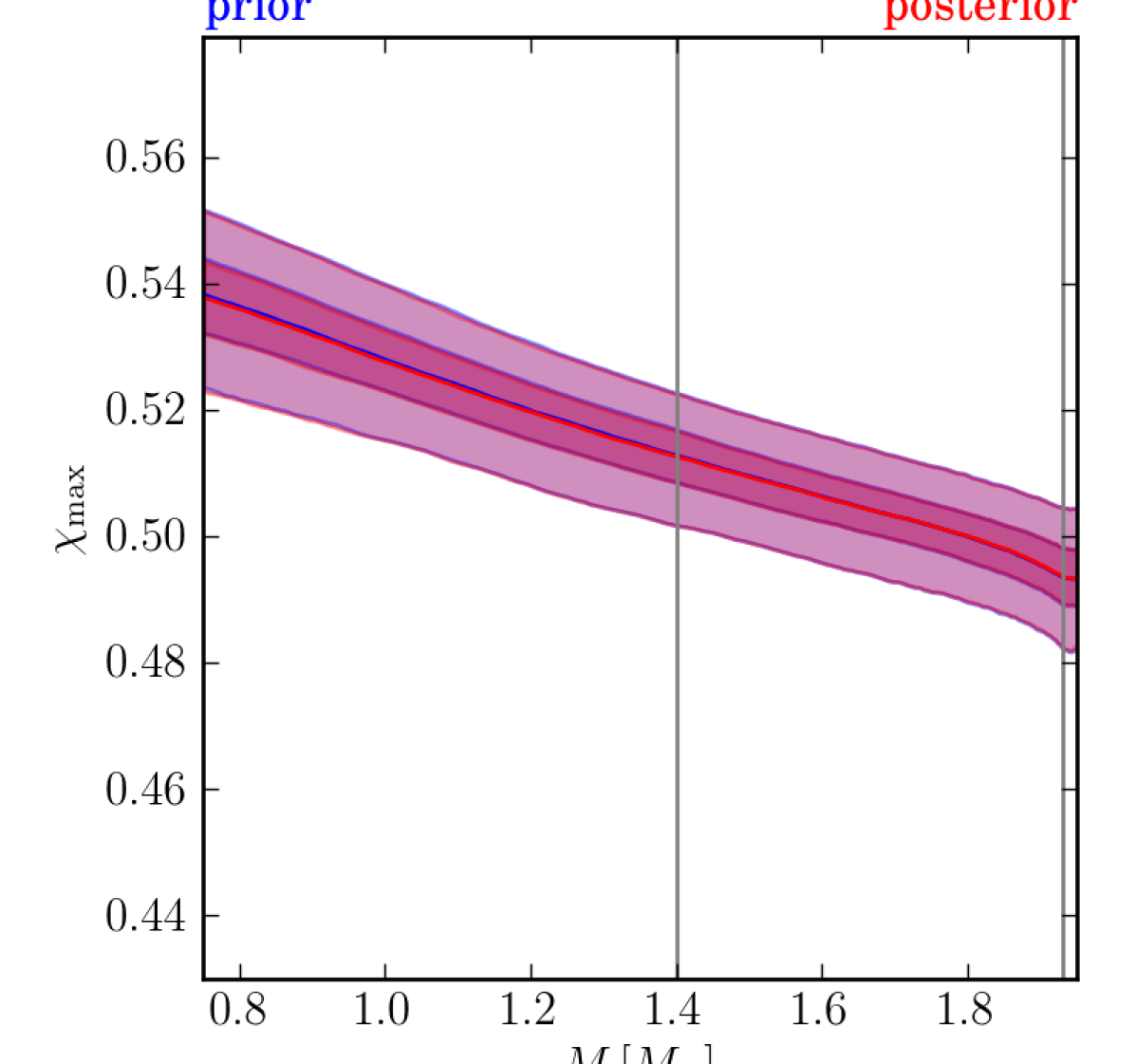
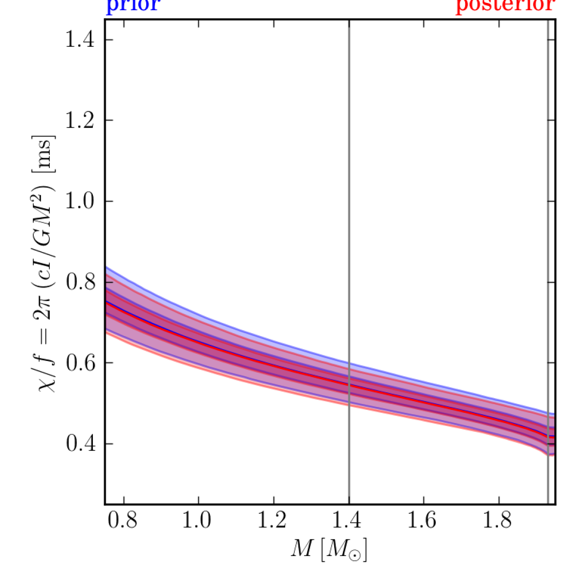
model-agnostic

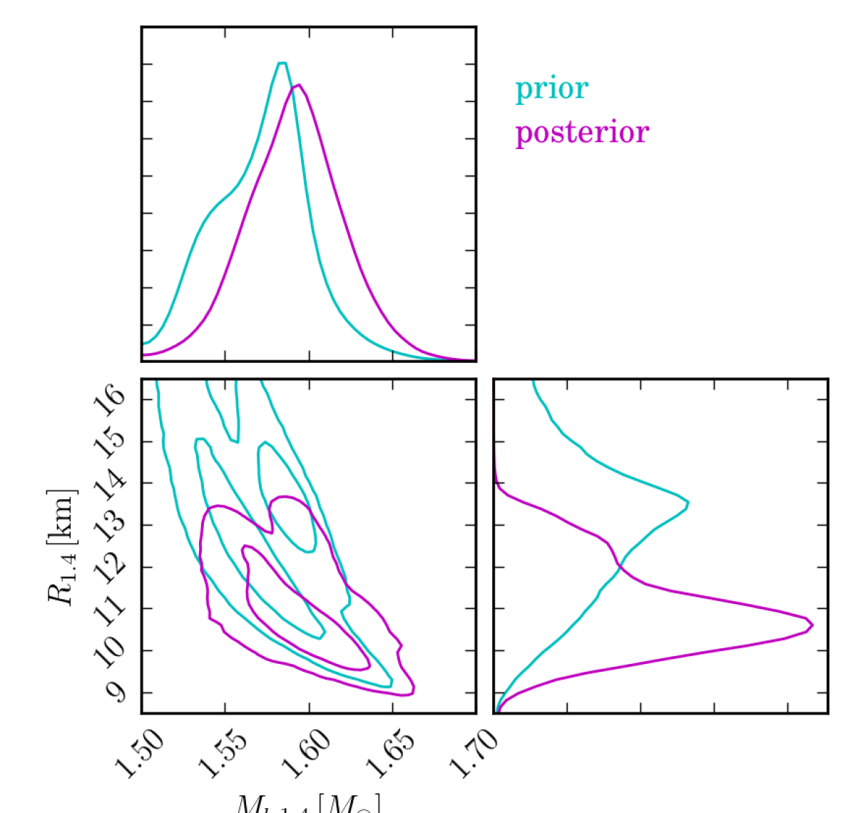
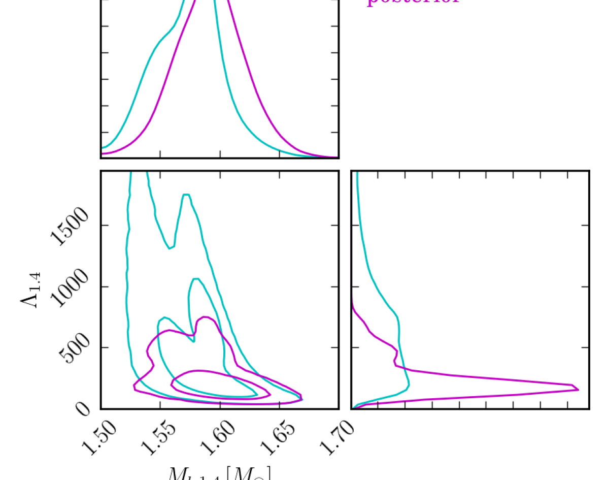
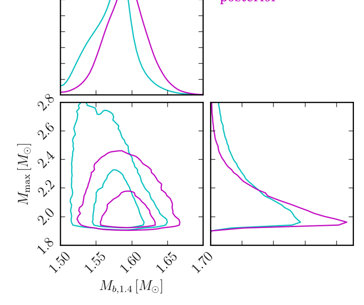
model-informed

Figure 7: Distributions for $M_{b,1.4}$, $M_{\mathrm{max}}$, $\Lambda_{1.4}$, and $R_{1.4}$ after marginalizing over EOS-composition. (Left) model-agnostic prior (cyan), posterior (magenta), and low-spin marginal-likelihood (green). (Right) model-informed prior (blue), posterior (red), and low-spin marginal-likelihood (green). Contours in the joint distributions denote minimal 50% and 90% credible regions. The bimodal behavior seen with the agnostic posterior is a combination of the inherited multimodal likelihood from GW170817 (see Figure 11 of Ref. Abbott and et al. (2019a)) as well as the preference for multiple stable branches. EOSs with multiple stable branches only inhabit the low-$R_{\mathrm{1.4}}$ mode, for example, while EOSs with a single stable branch inhabit both. The multimodal behavior seen with the informed prior is mostly due to the tight constraints imposed for each composition separately, which result in the separate peaks observed in these canonical observables.