Explicitly Bayesian Regularizations in Deep Learning

Xinjie Lan, Kenneth E. Barner
Department of Electrical and Computer Engineering
University of Delaware
Newark, DE 19713
lxjbit@udel.edu
Abstract

Generalization is essential for deep learning. In contrast to previous works claiming that Deep Neural Networks (DNNs) have an implicit regularization implemented by the stochastic gradient descent, we demonstrate explicitly Bayesian regularizations in a specific category of DNNs, i.e., Convolutional Neural Networks (CNNs). First, we introduce a novel probabilistic representation for the hidden layers of CNNs and demonstrate that CNNs correspond to Bayesian networks with the serial connection. Furthermore, we show that the hidden layers close to the input formulate prior distributions, thus CNNs have explicitly Bayesian regularizations based on the Bayesian regularization theory. In addition, we clarify two recently observed empirical phenomena that are inconsistent with traditional theories of generalization. Finally, we validate the proposed theory on a synthetic dataset.

1 Introduction

Generalization is a fundamental problem of deep learning theory. Since traditional generalization theories cannot clarify over-parameterized Deep Neural Networks (DNNs), especially in some cases, e.g., the random label classification [35, 20, 21], most recent works ascribe the generalization performance of DNNs to the Stochastic Gradient Descent (SGD) optimization implementing an implicit regularization, i.e., a bias towards models with low complexity [11, 3, 7, 30, 1].

Nevertheless, the implicit regularization explanations have lots of controversies. For example, Keskar et al. claim that the sharp minima learned by SGD lead to poor generalization [11], but Dinh et al. demonstrate that sharp minima can generalize DNNs well [3]. Sourdry et al. argue that SGD learns the minimum norm as the implicit regularization [7, 30], but Arora et al. doubt that the implicit regularization cannot be captured by the mathematical norm [1, 20].

In the context of regularization theories, Bayesian theory indicates that an explicit regularization can be formulated as a prior distribution [31]. However, it is scarce that explaining the regularization of DNNs from the Bayesian viewpoint, because the extremely complicated architecture of DNNs and the difficulty of probabilistic modeling high-dimensional activations impede establishing a comprehensive probabilistic explanation for the architecture of DNNs.

Numerous efforts have been devoted to explain the architecture of DNNs from a probabilistic perspective [29, 19, 25, 32, 26, 16, 18, 4, 24]. However, existing probabilistic explanations have several limitations. The Boltzmann explanations only clarify the restricted Boltzmann machine [29, 19]. The mixture model explanations require too strict assumptions [25, 32, 26]. The gaussian process explanations cannot clarify the hierarchical representation, an essential of deep learning [18]. In summary, existing explanations cannot establish a solid probabilistic foundation for investigating the regularization of DNNs from the Bayesian perspective.

To establish a solid probabilistic foundation for the study of Bayesian regularization in deep learning, we introduce a novel probabilistic representation for the hidden layers of Convolutional Neural Networks (CNNs) [13] by extending the Boltzmann explanation [19]. More specifically, a fully connected hidden layer formulate a multivariate discrete Boltzmann distribution [6], and its energy function is equal to the negative activations of the layer. In addition, a convolutional layer formulate a specific Boltzmann explanation, the Markov Random Fields (MRFs) model [5, 33], and its potential functions are determined by the linear convolutional filters.

Based on the proposed probabilistic representation, we demonstrate that CNNs formulate a directed acyclic graph, i.e., a Bayesian network [23, 12], and SGD learns the causality between the given training dataset and training labels. In the context of Bayesian networks, the causal links are described by conditional probabilities, thus the hidden layers close to the training dataset formulate prior distributions to describe the cause and the output layer formulates a probability to describe the expected effect. As a result, we conclude that CNNs have explicitly Bayesian regularizations based on the correspondence between prior distributions and regularizations.

We clarify two recently observed empirical phenomena that are inconsistent with traditional theories of generalization. First, increasing the number of hidden units can lead to a decrease in generalization error [21]. Bayesian theory indicates that CNNs can use more hidden units to generate a prior distribution including more prior knowledge, thereby achieving the lower generalization error. Second, CNNs with good generalization performance on real labels achieve zero training error but very high generalization error on random labels [35]. A Bayesian network can be simplified as two components, i.e., a prior distribution and a likelihood distribution, and regularization merely corresponds to the prior distribution. Given the same CNN architecture and the training dataset, CNNs should learn the same prior distributions to formulate the same regularization, different generalization errors result from the likelihood distribution but not related to the prior distribution, i.e., regularization.

2 Background

2.1 Boltzmann distribution

In mathematics, the Boltzmann distribution (a.k.a, the Gibbs distribution or the renormalization group) formulates the probability of a state, e.g., p​(𝒙;𝜽)π‘π’™πœ½p(\boldsymbol{x};\boldsymbol{\theta}), as a function of the state’s energy [6, 19, 34, 15].

p​(𝒙;𝜽)=1Z​(𝜽)​exp​[βˆ’E​(𝒙;𝜽)]​,π‘π’™πœ½1π‘πœ½expdelimited-[]πΈπ’™πœ½,{\textstyle p(\boldsymbol{x};\boldsymbol{\theta})=\frac{1}{Z(\boldsymbol{\theta})}\text{exp}[-E(\boldsymbol{x;\theta})]\text{,}} (1)

where E​(𝒙;𝜽)πΈπ’™πœ½E(\boldsymbol{x;\theta}) is the energy function, Z​(𝜽)=βˆ‘π’™exp​[βˆ’E​(𝒙;𝜽)]π‘πœ½subscript𝒙expdelimited-[]πΈπ’™πœ½Z(\boldsymbol{\theta})=\sum_{\boldsymbol{x}}{\text{exp}[-E(\boldsymbol{x;\theta})]} is the partition function, and 𝜽𝜽\boldsymbol{\theta} denote all parameters. A classical example of the Boltzmann distribution in machine learning is the Restricted Boltzmann Machine (RBM) [29].

The Boltzmann distribution can be reformulated as various probabilistic models through redefining the energy function E​(𝒙;𝜽)πΈπ’™πœ½E(\boldsymbol{x;\theta}). In the context of probabilistic graphical model, a fundamental Boltzmann distribution is the Markov Random Fields (MRFs) and its energy function is equivalent to the summation of multiple potential functions, i.e., E​(𝒙;𝜽)=βˆ’βˆ‘kfk​(𝒙;𝜽k)πΈπ’™πœ½subscriptπ‘˜subscriptπ‘“π‘˜π’™subscriptπœ½π‘˜{\scriptstyle E(\boldsymbol{x;\theta})=-\sum_{k}f_{k}(\boldsymbol{x};\boldsymbol{\theta}_{k})} [5, 33]. Moreover, assuming a single potential function defines an expert, i.e., 𝑭k=1Z​(𝜽k)​exp​[βˆ’fk​(𝒙;𝜽k)]subscriptπ‘­π‘˜1𝑍subscriptπœ½π‘˜expdelimited-[]subscriptπ‘“π‘˜π’™subscriptπœ½π‘˜{\scriptstyle\boldsymbol{F}_{k}=\frac{1}{Z(\boldsymbol{\theta}_{k})}\text{exp}[-f_{k}(\boldsymbol{x};\boldsymbol{\theta}_{k})]}, the Boltzmann distribution becomes a Product of Experts (PoE) model , i.e., p​(𝒙;𝜽)=1Z​(𝜽)β€‹βˆk𝑭kπ‘π’™πœ½1π‘πœ½subscriptproductπ‘˜subscriptπ‘­π‘˜{\scriptstyle p(\boldsymbol{x};\boldsymbol{\theta})=\frac{1}{Z(\boldsymbol{\theta})}\prod_{k}\boldsymbol{F}_{k}}, where Z​(𝜽)=∏kZ​(𝜽k)π‘πœ½subscriptproductπ‘˜π‘subscriptπœ½π‘˜{\scriptstyle Z(\boldsymbol{\theta})=\prod_{k}Z(\boldsymbol{\theta}_{k})} [9, 10].

2.2 Bayesian networks

A Bayesian network represents the causal probabilistic relationship among a set of random variables based on their conditional distributions. It consists of two major parts: a directed acyclic graph and a set of conditional probability distributions [23, 12]. For example, 𝑨→𝑩→𝑨𝑩\boldsymbol{A}\rightarrow\boldsymbol{B} forms a directed acyclic graph to show the possible causality between two random variables 𝑨𝑨\boldsymbol{A} and 𝑩𝑩\boldsymbol{B}, which can be formulated as P​(𝑨,𝑩)=P​(𝑩|𝑨)​P​(𝑨)𝑃𝑨𝑩𝑃conditional𝑩𝑨𝑃𝑨P(\boldsymbol{A},\boldsymbol{B})=P(\boldsymbol{B|A})P(\boldsymbol{A}), where P​(𝑨)𝑃𝑨P(\boldsymbol{A}) formulates a prior distribution to expresses the uncertainty of the cause and P​(𝑩|𝑨)𝑃conditional𝑩𝑨P(\boldsymbol{B|A}) formulates the uncertainty of the effect 𝑩𝑩\boldsymbol{B} given the cause 𝑨𝑨\boldsymbol{A}. In particular, since the prior distribution P​(𝑨)𝑃𝑨P(\boldsymbol{A}) expresses the prior belief of the cause that lead to the effect, P​(𝑨)𝑃𝑨P(\boldsymbol{A}) corresponds to the regularization in terms of the Bayesian regularization theory.

In this paper, we show that the entire architecture of CNNs forms a Bayesian network and the hidden layers close to the input formulate prior distributions to express the prior belief leading to the expected effect (i.e., labels), thus these hidden layers form explicitly Bayesian regularizations.

3 Main results

3.1 Preliminaries

We assume that 𝑿𝑿\boldsymbol{X} and 𝒀𝒀\boldsymbol{Y} are two random variables and Pπœ½β€‹(𝑿,𝒀)=P​(𝒀|𝑿)​P​(𝑿)subscriptπ‘ƒπœ½π‘Ώπ’€π‘ƒconditional𝒀𝑿𝑃𝑿P_{\boldsymbol{\theta}}(\boldsymbol{X},\boldsymbol{Y})=P(\boldsymbol{Y|X})P(\boldsymbol{X}) is an unknown joint distribution between 𝑿𝑿\boldsymbol{X} and 𝒀𝒀\boldsymbol{Y}, where P​(𝑿)𝑃𝑿P(\boldsymbol{X}) describes the prior knowledge of 𝑿𝑿\boldsymbol{X}, P​(𝒀|𝑿)𝑃conditional𝒀𝑿P(\boldsymbol{Y|X}) describes the statistical connection between 𝑿𝑿\boldsymbol{X} and 𝒀𝒀\boldsymbol{Y}, and 𝜽𝜽\boldsymbol{\theta} indicate the parameters of Pπœ½β€‹(𝑿,𝒀)subscriptπ‘ƒπœ½π‘Ώπ’€P_{\boldsymbol{\theta}}(\boldsymbol{X},\boldsymbol{Y}).

A dataset 𝓓={(𝒙j,π’šj)|𝒙jβˆˆβ„M,π’šjβˆˆβ„L}j=1J𝓓superscriptsubscriptconditional-setsuperscript𝒙𝑗superscriptπ’šπ‘—formulae-sequencesuperscript𝒙𝑗superscriptℝ𝑀superscriptπ’šπ‘—superscriptℝ𝐿𝑗1𝐽\boldsymbol{\mathcal{D}}=\{(\boldsymbol{x}^{j},\boldsymbol{y}^{j})|\boldsymbol{x}^{j}\in{\mathbb{R}}^{M},\boldsymbol{y}^{j}\in{\mathbb{R}}^{L}\}_{j=1}^{J} is composed of i.i.d. samples generated from Pθ​(𝑿,𝒀)subscriptπ‘ƒπœƒπ‘Ώπ’€P_{\theta}(\boldsymbol{X},\boldsymbol{Y}). In addition, a CNN with I𝐼I hidden layers is denoted as CNN={𝒙;π’‡πŸ;…;𝒇𝑰;𝒇𝒀}CNN𝒙subscript𝒇1bold-…subscript𝒇𝑰subscript𝒇𝒀\text{CNN}=\{\boldsymbol{x;f_{1};...;f_{I};f_{Y}}\} and trained by 𝓓𝓓\boldsymbol{\mathcal{D}}, where (𝒙,π’š)βˆˆπ““π’™π’šπ““(\boldsymbol{x},\boldsymbol{y})\in\boldsymbol{\mathcal{D}} are the input of the CNN and the corresponding training label, and 𝒇𝒀subscript𝒇𝒀\boldsymbol{f_{Y}} is an estimation of the true distribution P​(𝒀|𝑿)𝑃conditional𝒀𝑿P(\boldsymbol{Y|X}). As a result, π’™βˆΌP​(𝑿)similar-to𝒙𝑃𝑿\boldsymbol{x}\sim P(\boldsymbol{X}) and π’‡π’€β‰ˆP​(𝒀|𝑿)subscript𝒇𝒀𝑃conditional𝒀𝑿\boldsymbol{f_{Y}}\approx P(\boldsymbol{Y|X}).

3.2 The probabilistic representation for the hidden layers of CNNs

In this section, we extend the Boltzmann explanations to CNNs and introduce a novel probabilistic representation for the hidden layers of CNNs. The detailed derivation is included in Appendix 6.1. Since most CNNs only contain two categories of hidden layers, namely fully connected layers and convolutional layers with non-linear operators, e.g., ReLU and pooling, the proposed probabilistic representation can be summarized as the following propositions.

Proposition 1: A fully connected layer formulates a multivariate discrete Boltzmann distribution and the energy function of which is equivalent to the negative activations of the fully connected layer.

A fully connected layer π’‡π’Š={fi​n}n=1Nsubscriptπ’‡π’Šsuperscriptsubscriptsubscript𝑓𝑖𝑛𝑛1𝑁\boldsymbol{f_{i}}=\{f_{in}\}_{n=1}^{N} with N𝑁N neurons formulates a multivariate discrete Boltzmann distribution to describe the probability of N𝑁N features defined by the neurons occurring in the input. Their energy functions are equal to the negative of their respective neurons, i.e., Efi​n=βˆ’fi​n​(𝒇𝒋)subscript𝐸subscript𝑓𝑖𝑛subscript𝑓𝑖𝑛subscript𝒇𝒋E_{f_{in}}=-f_{in}(\boldsymbol{f_{j}}).

P​(π‘­π’Š)={P​(fi​n)=1Zπ‘­π’Šβ€‹exp​[fi​n​(𝒇𝒋)]}n=1N𝑃subscriptπ‘­π’Šsuperscriptsubscript𝑃subscript𝑓𝑖𝑛1subscript𝑍subscriptπ‘­π’Šexpdelimited-[]subscript𝑓𝑖𝑛subscript𝒇𝒋𝑛1𝑁P(\boldsymbol{F_{i}})=\{P(f_{in})=\frac{1}{Z_{\boldsymbol{F_{i}}}}\text{exp}[f_{in}(\boldsymbol{f_{j}})]\}_{n=1}^{N} (2)

where the previous layer 𝒇𝒋={fj​m}m=1Msubscript𝒇𝒋superscriptsubscriptsubscriptπ‘“π‘—π‘šπ‘š1𝑀\boldsymbol{f_{j}}=\{f_{jm}\}_{m=1}^{M} is the input, fi​n​(𝒇𝒋)=σ​[gi​n​(𝒇𝒋)]subscript𝑓𝑖𝑛subscriptπ’‡π’‹πœŽdelimited-[]subscript𝑔𝑖𝑛subscript𝒇𝒋f_{in}(\boldsymbol{f_{j}})=\sigma[g_{in}(\boldsymbol{f_{j}})] is the activation of the n𝑛nth neuron, gi​n​(𝒇𝒋)=βˆ‘m=1MΞ±m​nβ‹…fj​m+bi​nsubscript𝑔𝑖𝑛subscript𝒇𝒋superscriptsubscriptπ‘š1𝑀⋅subscriptπ›Όπ‘šπ‘›subscriptπ‘“π‘—π‘šsubscript𝑏𝑖𝑛{g_{in}(\boldsymbol{f_{j}})=\sum_{m=1}^{M}\alpha_{mn}\cdot f_{jm}+b_{in}} is a linear filter with Ξ±m​nsubscriptπ›Όπ‘šπ‘›\alpha_{mn} being the weights and bi​nsubscript𝑏𝑖𝑛b_{in} being the bias, σ​(β‹…)πœŽβ‹…\sigma(\cdot) is an activation function, and Z𝑭=βˆ‘n=1Nexp​[fi​n​(𝒇𝒋)]subscript𝑍𝑭superscriptsubscript𝑛1𝑁expdelimited-[]subscript𝑓𝑖𝑛subscript𝒇𝒋{Z_{\boldsymbol{F}}=\sum_{n=1}^{N}\text{exp}[f_{in}(\boldsymbol{f_{j}})]} is the partition function.

Proposition 2: A convolutional layer formulates a specific Boltzmann distribution, i.e., the MRF model, and its energy function is equal to the negative summation of all the convolutional channels.

A convolutional layer with N𝑁N convolutional channels, i.e., π’‡π’Š={π’‡π’Šπ’=σ​(Ο†in​(𝒇𝒋))}n=1Nsubscriptπ’‡π’Šsuperscriptsubscriptsubscriptsuperscriptπ’‡π’π’ŠπœŽsuperscriptsubscriptπœ‘π‘–π‘›subscript𝒇𝒋𝑛1𝑁\boldsymbol{f_{i}}=\{\boldsymbol{f^{n}_{i}}=\sigma(\varphi_{i}^{n}(\boldsymbol{f_{j}}))\}_{n=1}^{N}, formulates a specific Boltzmann distribution, namely a MRF model.

P​(π‘­π’Š)=1Zπ‘­π’Šβ€‹exp​[βˆ‘n=1NΟ†in​(𝒇𝒋)]𝑃subscriptπ‘­π’Š1subscript𝑍subscriptπ‘­π’Šexpdelimited-[]superscriptsubscript𝑛1𝑁superscriptsubscriptπœ‘π‘–π‘›subscript𝒇𝒋P(\boldsymbol{F_{i}})=\frac{1}{Z_{\boldsymbol{F_{i}}}}\text{exp}[\sum_{n=1}^{N}\varphi_{i}^{n}(\boldsymbol{f_{j}})] (3)

where 𝒇𝒋={𝒇𝒋𝒒}q=1Qsubscript𝒇𝒋superscriptsubscriptsuperscriptsubscriptπ’‡π’‹π’’π‘ž1𝑄\boldsymbol{f_{j}}=\{\boldsymbol{f_{j}^{q}}\}_{q=1}^{Q} is the input with Q𝑄Q channels, Ο†in(𝒇𝒋)=βˆ‘q=1Q𝑺(𝒏,𝒒)βˆ˜π’‡π’‹π’’+binβ‹…πŸ)\varphi_{i}^{n}(\boldsymbol{f_{j}})=\sum_{q=1}^{Q}\boldsymbol{S^{(n,q)}}\circ\boldsymbol{f_{j}^{q}}+b_{i}^{n}\cdot\boldsymbol{1}) is the n𝑛nth linear convolutional channel corresponding to the potential function of a MRF model, in which 𝑺(𝒏,𝒒)superscript𝑺𝒏𝒒\boldsymbol{S^{(n,q)}} is the n𝑛nth convolutional filter applying to the qπ‘žqth channel, binsuperscriptsubscript𝑏𝑖𝑛b_{i}^{n} is the bias, σ​(β‹…)πœŽβ‹…\sigma(\cdot) is an non-linear operator, and the partition function Zπ‘­π’Š=βˆ«π’‡π’‹exp​[βˆ‘n=1NΟ†in​(𝒇𝒋)]​𝑑𝒇𝒋subscript𝑍subscriptπ‘­π’Šsubscriptsubscript𝒇𝒋expdelimited-[]superscriptsubscript𝑛1𝑁superscriptsubscriptπœ‘π‘–π‘›subscript𝒇𝒋differential-dsubscript𝒇𝒋Z_{\boldsymbol{F_{i}}}=\int_{\boldsymbol{f_{j}}}\text{exp}[\sum_{n=1}^{N}\varphi_{i}^{n}(\boldsymbol{f_{j}})]d{\boldsymbol{f_{j}}}. In particular, based on the equivalence between SGD and the first order approximation [2], Equation 3 indicates that the statistical property of a convolutional layer is determined by the linear convolutional operations {Ο†in​(𝒇𝒋)}n=1Nsuperscriptsubscriptsuperscriptsubscriptπœ‘π‘–π‘›subscript𝒇𝒋𝑛1𝑁\{\varphi_{i}^{n}(\boldsymbol{f_{j}})\}_{n=1}^{N}.

In summary, the Boltzmann distribution establishes a novel connection between the hidden layers of CNNs and probabilistic models through defining the energy function of a Boltzmann distribution as a function of the activations in a hidden layer. It is important to note that the energy function is a sufficient statistics of a Boltzmann distribution, i.e., the later is entirely dependent on the former [22]. As a result, we can specify a unique Boltzmann distribution given a hidden layer of CNNs.

Moreover, the architecture of hidden layers determines the statistical property of the corresponding Boltzmann distribution. For example, a fully connected layer assumes all the input data being connected to each other, but a convolutional layer assumes local connectivity, i.e., the input data only depends on its neighbors. Therefore, their corresponding Boltzmann distributions have different statistical properties: Equation 2 uses the linear filter gi​n​(𝒇𝒋)subscript𝑔𝑖𝑛subscript𝒇𝒋g_{in}(\boldsymbol{f_{j}}) to describe the fully connected features, and Equation 3 uses the potential functions of MRF to model the local connected features.

3.3 Explicitly Bayesian regularizations in CNNs

Proposition 3: The entire architecture of CNNs can be explained as a Bayesian network.

Given a CNN={𝒙;π’‡πŸ;…;𝒇𝑰;𝒇𝒀}CNN𝒙subscript𝒇1bold-…subscript𝒇𝑰subscript𝒇𝒀\text{CNN}=\{\boldsymbol{x;f_{1};...;f_{I};f_{Y}}\}, the output of the hidden layer π’‡π’Šsubscriptπ’‡π’Š\boldsymbol{f_{i}} is the input of the next hidden layer π’‡π’Š+𝟏subscriptπ’‡π’Š1\boldsymbol{f_{i+1}}, thus the CNN forms a serial connection in terms of Bayesian networks.

π’‡πŸβ†’β‹―β†’π’‡π‘°β†’π’‡π’€bold-β†’subscript𝒇1bold-β‹―bold-β†’subscript𝒇𝑰bold-β†’subscript𝒇𝒀\boldsymbol{f_{1}\rightarrow\cdots\rightarrow f_{I}\rightarrow f_{Y}} (4)

Since the proposed probabilistic representation specifies the distribution of the hidden layers of CNNs, the entire architecture of the CNN corresponds to a Bayesian network as

P​(𝑭𝒀;𝑭𝑰;β‹―;π‘­πŸ|𝑿)=P​(𝑭𝒀|𝑭𝑰)⋅…⋅P​(π‘­π’Š+𝟏|π‘­π’Š)⋅…⋅P​(π‘­πŸ|𝑿)𝑃subscript𝑭𝒀subscript𝑭𝑰bold-β‹―conditionalsubscript𝑭1𝑿⋅⋅𝑃conditionalsubscript𝑭𝒀subscript𝑭𝑰…𝑃conditionalsubscriptπ‘­π’Š1subscriptπ‘­π’Šβ€¦π‘ƒconditionalsubscript𝑭1𝑿{\textstyle P(\boldsymbol{F_{Y};F_{I};\cdots;F_{1}|X})=P(\boldsymbol{F_{Y}|F_{I}})\cdot...\cdot P(\boldsymbol{F_{i+1}|F_{i}})\cdot...\cdot P(\boldsymbol{F_{1}|X})} (5)

where P​(π‘­πŸ|𝑿)𝑃conditionalsubscript𝑭1𝑿P(\boldsymbol{F_{1}|X}) formulates a prior Boltzmann distribution to describe the cause, the P​(𝑭𝒀|𝑭𝑰)𝑃conditionalsubscript𝑭𝒀subscript𝑭𝑰P(\boldsymbol{F_{Y}|F_{I}}) formulates a Boltzmann distribution to express the expected effect, and the intermediate hidden layers formulate multiple conditional distributions to transfer the influence of the cause to the effect.

Previous works demonstrate that the output of CNNs estimates a Bayesian posterior distribution P​(𝑭𝒀|𝑿)𝑃conditionalsubscript𝑭𝒀𝑿P(\boldsymbol{F_{Y}|X}) [27, 36]. In the context of Bayesian networks, P​(𝑭𝒀|𝑿)𝑃conditionalsubscript𝑭𝒀𝑿P(\boldsymbol{F_{Y}|X}) can be explained as a variable inference given the Bayesian networks corresponding to CNNs.

P(𝑭𝒀|𝑿)=βˆ«π‘­π‘°β‹―βˆ«π‘­πŸP(𝑭𝒀;𝑭𝑰..;π‘­πŸ|𝑿)d𝑭𝑰⋯dπ‘­πŸP(\boldsymbol{F_{Y}|X})=\int_{\boldsymbol{F_{I}}}\cdots\int_{\boldsymbol{F_{1}}}P(\boldsymbol{F_{Y};F_{I}..;F_{1}|X})d{\boldsymbol{F_{I}}}\cdots d{\boldsymbol{F_{1}}} (6)

Since CNNs form a Bayesian network with the serial connection and the distribution of each layer is a Boltzmann distribution, we prove that P​(𝑭𝒀|𝑿)𝑃conditionalsubscript𝑭𝒀𝑿P(\boldsymbol{F_{Y}|X}) is also a Boltzmann distribution and the energy function of which is also equivalent to the functionality of the entire CNN in Appendix 6.2.

Given the training dataset 𝓓𝓓\boldsymbol{\mathcal{D}} and a predefined loss function, e.g., the cross entropy, SGD can be explained as a parameter learning procedure for P​(𝑭𝒀|𝑿)𝑃conditionalsubscript𝑭𝒀𝑿P(\boldsymbol{F_{Y}|X}). Notably, since CNNs form a serial connection indicated by Equation 4, both the Bayesian posterior distribution P​(𝑭𝒀|𝑿)𝑃conditionalsubscript𝑭𝒀𝑿P(\boldsymbol{F_{Y}|X}) and the entire Bayesian network P(𝑭𝒀;𝑭𝑰..;π‘­πŸ|𝑿)P(\boldsymbol{F_{Y};F_{I}..;F_{1}|X}) correspond to the same architecture of CNNs, thus SGD can learn the parameters of the entire Bayesian network by merely optimizing P​(𝑭𝒀|𝑿)𝑃conditionalsubscript𝑭𝒀𝑿P(\boldsymbol{F_{Y}|X}).

Proposition 4: CNNs have explicitly Bayesian regularizations

In the Bayesian approach, regularization is achieved by specifying a prior distribution over the parameters and subsequently averaging over the posterior distribution [31]. Therefore, the Bayesian networks explanation provides a novel perspective to clarify the generalization of CNNs.

Above all, CNNs have explicitly Bayesian regularizations. Since we explain the entire architecture of CNNs as a Bayesian network with the serial connection indicated by Equation 4, the hidden layers close to the input should formulate prior distributions, thereby representing explicit regularizations. In contrast to previous works ascribing the generalization of CNNs to SGD implementing implicit regularization, Proposition 3 shows that SGD merely serves as a parameter learning for P​(𝑭𝒀|𝑿)𝑃conditionalsubscript𝑭𝒀𝑿P(\boldsymbol{F_{Y}|X}) and explicit Bayesian regularizations are defined by the hidden layers corresponding to prior distributions.

Moreover, the Bayesian regularization explanation can clarify several recently observed empirical phenomena that are inconsistent with traditional theories of generalization [20]. First, increasing the number of hidden units of CNNs, i.e., increasing the number of parameters, can lead to a decrease in generalization error [21]. Bayesian theory indicates that more complex prior distributions can include more prior belief of the training dataset. As a result, CNNs can use many hidden units to generate much powerful prior distributions for regularizing the entire network, thereby guaranteeing the generalization performance though they are over-parametrized.

Second, CNNs with good generalization performance on real labels achieve zero training error but very high generalization error on random labels [35]. Bayesian theory enables us to utilize the β€˜separate and conquer’ rule to understand the special case. In terms of Bayesian theory, a Bayesian network can be simplified as two components, namely a prior distribution and a likelihood distribution. Given the same CNN architecture and the same training dataset with different labels, e.g., real labels and random labels, the CNN should formulate the same regularizations, because regularization merely corresponds the prior distribution. Different generalization errors for different labels result from the learned likelihood distribution but not related to the prior distribution.

4 Simulations

In this section, we use a synthetic dataset to validate explicitly Bayesian regularizations in CNNs, and demonstrate that the proposed Bayesian regularization can explain two noteworthy empirical phenomena that are inconsistent with traditional theories of generalization.

4.1 Setup
Refer to caption
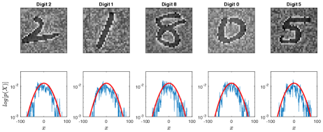
Figure 1: The first row shows five synthetic images of handwritten digits, the second row shows their respective empirical distributions, and the red curve indicates the true distribution 𝒩​(0,1024)𝒩01024\mathcal{N}(0,1024).

To validate explicitly Bayesian regularizations in CNNs, we need to firstly validate the probabilistic representation for the hidden layers of CNNs. However, since the distributions of benchmark datasets are unknown, it is impossible to directly use them to validate the proposed probabilistic representation. Alternatively, we generate a synthetic dataset obeying the Gaussian distribution 𝒩​(0,1024)𝒩01024\mathcal{N}(0,1024) based on the NIST dataset of handwritten digits [14]. It consists of 20,000 32Γ—32323232\times 32 grayscale images in 10 classes (digits from 0 to 9), and each class has 1,000 training images and 1,000 testing images. The method for generating the synthetic dataset is included in Appendix 6.3.

Most image datasets satisfy two fundamental assumptions: stationary and Markov [17]. The former means that the distribution is independent on the location, i.e., the distribution of pixels at different locations are identically distributed. The later indicates that the distribution of a single pixel is independent on the other pixels given its neighbors. The two assumptions allow us to use an empirical distribution to simulate the true distribution of the synthetic dataset. Figure 1 shows five synthetic images and their perspective empirical distributions. It shows that their empirical distributions precisely simulate the true distribution of synthetic images, i.e., 𝒩​(0,1024)𝒩01024\mathcal{N}(0,1024).

We design three simple by comprehensive CNNs for classifying the synthetic dataset. Every CNN has two convolutional hidden layers, two max pooling layers, and a fully connected hidden layer. The only difference within these CNNs is that the first convolutional layer π’‡πŸsubscript𝒇1\boldsymbol{f_{1}} of different CNNs has different number of convolutional channels.

Table 1: The architectures of CNNs for classifying the synthetic dataset
R.V. Layer Description CNN1 CNN2 CNN3
𝑿𝑿\boldsymbol{X} 𝒙𝒙\boldsymbol{x} Input 32Γ—32Γ—13232132\times 32\times 1 32Γ—32Γ—13232132\times 32\times 1 32Γ—32Γ—13232132\times 32\times 1
π‘­πŸsubscript𝑭1\boldsymbol{F_{1}} π’‡πŸsubscript𝒇1\boldsymbol{f_{1}} Conv (3Γ—3333\times 3) +ReLU 30Γ—30Γ—πŸ’3030430\times 30\times\boldsymbol{4} 30Γ—30Γ—πŸπŸ30301230\times 30\times\boldsymbol{12} 30Γ—30Γ—πŸπŸŽ30302030\times 30\times\boldsymbol{20}
π’‡πŸsubscript𝒇2\boldsymbol{f_{2}} Maxpool 15Γ—15Γ—41515415\times 15\times{4} 15Γ—15Γ—1215151215\times 15\times 12 15Γ—15Γ—2015152015\times 15\times 20
π‘­πŸsubscript𝑭2\boldsymbol{F_{2}} π’‡πŸ‘subscript𝒇3\boldsymbol{f_{3}} Conv (5Γ—5555\times 5) + ReLU 11Γ—11Γ—2011112011\times 11\times 20 11Γ—11Γ—2011112011\times 11\times 20 11Γ—11Γ—2011112011\times 11\times 20
π’‡πŸ’subscript𝒇4\boldsymbol{f_{4}} Maxpool 5Γ—5Γ—2055205\times 5\times{20} 5Γ—5Γ—2055205\times 5\times 20 5Γ—5Γ—2055205\times 5\times 20
π‘­πŸ‘subscript𝑭3\boldsymbol{F_{3}} π’‡πŸ“subscript𝒇5\boldsymbol{f_{5}} Fully connected 1Γ—1Γ—2011201\times 1\times 20 1Γ—1Γ—2011201\times 1\times 20 1Γ—1Γ—2011201\times 1\times 20
𝑭𝒀subscript𝑭𝒀\boldsymbol{F_{Y}} 𝒇𝒀subscript𝒇𝒀\boldsymbol{f_{Y}} Output(softmax) 1Γ—1Γ—1011101\times 1\times 10 1Γ—1Γ—1011101\times 1\times 10 1Γ—1Γ—1011101\times 1\times 10
  • β€’

    R.V. is the random variable of the hidden layer(s).

Based on the proposed probabilistic representation, we identify the distribution of each hidden layer in the above CNNs={𝒙;π’‡πŸ;…;𝒇𝑰;𝒇𝒀}CNNs𝒙subscript𝒇1bold-…subscript𝒇𝑰subscript𝒇𝒀\text{CNNs}=\{\boldsymbol{x;f_{1};...;f_{I};f_{Y}}\}. First, π’‡πŸsubscript𝒇1\boldsymbol{f_{1}} formulates a specific Boltzmann distribution, namely, a MRF model. Since the max pooling layer π’‡πŸsubscript𝒇2\boldsymbol{f_{2}} can be viewed as an non-linear differentiable operation as ReLU, the distribution of π’‡πŸsubscript𝒇2\boldsymbol{f_{2}} can be approximated by π’‡πŸsubscript𝒇1\boldsymbol{f_{1}} based on the equivalence between SGD and the first order approximation [2]. Therefore, we can use a single random variable π‘­πŸsubscript𝑭1\boldsymbol{F_{1}} to represent the statistical properties of both π’‡πŸsubscript𝒇1\boldsymbol{f_{1}} and π’‡πŸsubscript𝒇2\boldsymbol{f_{2}}. Similarly, we use π‘­πŸsubscript𝑭2\boldsymbol{F_{2}} to represent the statistical properties of both π’‡πŸ‘subscript𝒇3\boldsymbol{f_{3}} and π’‡πŸ’subscript𝒇4\boldsymbol{f_{4}}. As a result, P​(π‘­πŸ)𝑃subscript𝑭1P(\boldsymbol{F_{1}}) and P​(π‘­πŸ|π‘­πŸ)𝑃conditionalsubscript𝑭2subscript𝑭1P(\boldsymbol{F_{2}|F_{1}}) can be formulated as

P​(π‘­πŸ)=1Zπ‘­πŸβ€‹exp​[βˆ‘n=1NΟ†1n​(𝒙)]​ and ​P​(π‘­πŸ|π‘­πŸ)=1Zπ‘­πŸβ€‹exp​[βˆ‘k=1KΟ†3k​(π’‡πŸ)]𝑃subscript𝑭11subscript𝑍subscript𝑭1expdelimited-[]superscriptsubscript𝑛1𝑁superscriptsubscriptπœ‘1𝑛𝒙 and 𝑃conditionalsubscript𝑭2subscript𝑭11subscript𝑍subscript𝑭2expdelimited-[]superscriptsubscriptπ‘˜1𝐾superscriptsubscriptπœ‘3π‘˜subscript𝒇2\begin{split}P(\boldsymbol{F_{1}})=\frac{1}{Z_{\boldsymbol{F_{1}}}}\text{exp}[\sum_{n=1}^{N}\varphi_{1}^{n}(\boldsymbol{x})]\text{ and }P(\boldsymbol{F_{2}|F_{1}})=\frac{1}{Z_{\boldsymbol{F_{2}}}}\text{exp}[\sum_{k=1}^{K}\varphi_{3}^{k}(\boldsymbol{f_{2}})]\end{split} (7)

where 𝒙𝒙\boldsymbol{x} only has a single channel since it denotes a gray scale image, and Ο†1n​(𝒙)=π‘ΊπŸπ’βˆ˜π’™+b1nβ‹…πŸsuperscriptsubscriptπœ‘1𝑛𝒙superscriptsubscript𝑺1𝒏𝒙⋅superscriptsubscript𝑏1𝑛1\varphi_{1}^{n}(\boldsymbol{x})=\boldsymbol{S_{1}^{n}}\circ\boldsymbol{x}+b_{1}^{n}\cdot\boldsymbol{1} is the n𝑛nth linear convolutional channel in π’‡πŸsubscript𝒇1\boldsymbol{f_{1}}. Similarly, π’‡πŸ={π’‡πŸπ’}n=1Nsubscript𝒇2superscriptsubscriptsubscriptsuperscript𝒇𝒏2𝑛1𝑁\boldsymbol{f_{2}}=\{\boldsymbol{f^{n}_{2}}\}_{n=1}^{N} has N𝑁N channels, and Ο†3k(π’‡πŸ)=βˆ‘n=1Nπ‘ΊπŸ‘(π’Œ,𝒏)βˆ˜π’‡πŸπ’Œ+b2kβ‹…πŸ)\varphi_{3}^{k}(\boldsymbol{f_{2}})=\sum_{n=1}^{N}\boldsymbol{S_{3}^{(k,n)}}\circ\boldsymbol{f_{2}^{k}}+b_{2}^{k}\cdot\boldsymbol{1}) is the kπ‘˜kth linear convolutional channel in π’‡πŸ‘subscript𝒇3\boldsymbol{f_{3}}. The two partition functions are Zπ‘­πŸ=βˆ«π’™exp​[βˆ‘n=1NΟ†1n​(𝒙)]​𝑑𝒙subscript𝑍subscript𝑭1subscript𝒙expdelimited-[]superscriptsubscript𝑛1𝑁superscriptsubscriptπœ‘1𝑛𝒙differential-d𝒙Z_{\boldsymbol{F_{1}}}=\int_{\boldsymbol{x}}\text{exp}[\sum_{n=1}^{N}\varphi_{1}^{n}(\boldsymbol{x})]d{\boldsymbol{x}} and Zπ‘­πŸ=βˆ«π’‡πŸexp​[βˆ‘k=1KΟ†3k​(π’‡πŸ)]β€‹π‘‘π’‡πŸsubscript𝑍subscript𝑭2subscriptsubscript𝒇2expdelimited-[]superscriptsubscriptπ‘˜1𝐾superscriptsubscriptπœ‘3π‘˜subscript𝒇2differential-dsubscript𝒇2Z_{\boldsymbol{F_{2}}}=\int_{\boldsymbol{f_{2}}}\text{exp}[\sum_{k=1}^{K}\varphi_{3}^{k}(\boldsymbol{f_{2}})]d{\boldsymbol{f_{2}}}.

Although we derive P​(π‘­πŸ)𝑃subscript𝑭1P(\boldsymbol{F_{1}}) and P​(π‘­πŸ|π‘­πŸ)𝑃conditionalsubscript𝑭2subscript𝑭1P(\boldsymbol{F_{2}|F_{1}}), it is still hard to calculate P​(π‘­πŸ)𝑃subscript𝑭1P(\boldsymbol{F_{1}}) and P​(π‘­πŸ|π‘­πŸ)𝑃conditionalsubscript𝑭2subscript𝑭1P(\boldsymbol{F_{2}|F_{1}}) because Zπ‘­πŸsubscript𝑍subscript𝑭1Z_{\boldsymbol{F_{1}}} and Zπ‘­πŸsubscript𝑍subscript𝑭2Z_{\boldsymbol{F_{2}}} are intractable for the high dimensional datasets 𝒙𝒙\boldsymbol{x} and π’‡πŸsubscript𝒇2\boldsymbol{f_{2}}. Alternatively, since MRF models satisfy the two assumptions (i.e., stationary and Markov) and the energy function is a sufficient statistics of a Boltzmann distribution, we can use the empirical distributions of their respective energy functions (π‘¬π‘­πŸ=βˆ’βˆ‘n=1NΟ†1n​(𝒙)subscript𝑬subscript𝑭1superscriptsubscript𝑛1𝑁superscriptsubscriptπœ‘1𝑛𝒙{\scriptstyle\boldsymbol{E}_{\boldsymbol{F_{1}}}=-\sum_{n=1}^{N}\varphi_{1}^{n}(\boldsymbol{x})} and π‘¬π‘­πŸ=βˆ’βˆ‘k=1KΟ†2k​(π’‡πŸ)subscript𝑬subscript𝑭2superscriptsubscriptπ‘˜1𝐾superscriptsubscriptπœ‘2π‘˜subscript𝒇2{\scriptstyle\boldsymbol{E}_{\boldsymbol{F_{2}}}=-\sum_{k=1}^{K}\varphi_{2}^{k}(\boldsymbol{f_{2}})}) to estimate P​(π‘­πŸ)𝑃subscript𝑭1P(\boldsymbol{F_{1}}) and P​(π‘­πŸ|π‘­πŸ)𝑃conditionalsubscript𝑭2subscript𝑭1P(\boldsymbol{F_{2}|F_{1}}). Specifically, the two empirical distributions can be expressed as

P^​[π‘­πŸβ€‹(Bi)]=1Cπ‘¬π‘­πŸβ€‹[βˆ‘n​n=1Cπ‘¬π‘­πŸBiβ‰€πŸβ€‹[π‘¬π‘­πŸβ€‹(n​n)]≀Bi+1]P^​[π‘­πŸ|π‘­πŸβ€‹(Bi)]=1Cπ‘¬π‘­πŸβ€‹[βˆ‘m​m=1Cπ‘¬π‘­πŸBiβ‰€πŸβ€‹[π‘¬π‘­πŸβ€‹(m​m)]≀Bi+1]^𝑃delimited-[]subscript𝑭1subscript𝐡𝑖1subscript𝐢subscript𝑬subscript𝑭1delimited-[]superscriptsubscript𝑛𝑛1subscript𝐢subscript𝑬subscript𝑭1subscript𝐡𝑖1delimited-[]subscript𝑬subscript𝑭1𝑛𝑛subscript𝐡𝑖1^𝑃delimited-[]conditionalsubscript𝑭2subscript𝑭1subscript𝐡𝑖1subscript𝐢subscript𝑬subscript𝑭2delimited-[]superscriptsubscriptπ‘šπ‘š1subscript𝐢subscript𝑬subscript𝑭2subscript𝐡𝑖1delimited-[]subscript𝑬subscript𝑭2π‘šπ‘šsubscript𝐡𝑖1\begin{split}\hat{P}[\boldsymbol{F_{1}}(B_{i})]=\frac{1}{C_{\boldsymbol{E}_{\boldsymbol{F_{1}}}}}[\sum_{nn=1}^{C_{\boldsymbol{E}_{\boldsymbol{F_{1}}}}}B_{i}\leq\boldsymbol{1}[\boldsymbol{E}_{\boldsymbol{F_{1}}}(nn)]\leq B_{i+1}]\\ \hat{P}[\boldsymbol{F_{2}|F_{1}}(B_{i})]=\frac{1}{C_{\boldsymbol{E}_{\boldsymbol{F_{2}}}}}[\sum_{mm=1}^{C_{\boldsymbol{E}_{\boldsymbol{F_{2}}}}}B_{i}\leq\boldsymbol{1}[\boldsymbol{E}_{\boldsymbol{F_{2}}}(mm)]\leq B_{i+1}]\end{split} (8)

where Cπ‘¬π‘­πŸsubscript𝐢subscript𝑬subscript𝑭1C_{\boldsymbol{E}_{\boldsymbol{F_{1}}}} and Cπ‘¬π‘­πŸsubscript𝐢subscript𝑬subscript𝑭2C_{\boldsymbol{E}_{\boldsymbol{F_{2}}}} are the number of elements in π‘¬π‘­πŸsubscript𝑬subscript𝑭1\boldsymbol{E}_{\boldsymbol{F_{1}}} and π‘¬π‘­πŸsubscript𝑬subscript𝑭2\boldsymbol{E}_{\boldsymbol{F_{2}}}, respectively. Bisubscript𝐡𝑖B_{i} and Bi+1subscript𝐡𝑖1B_{i+1} are the pre-defined edges, and πŸβ€‹(β‹…)1β‹…\boldsymbol{1}(\cdot) is the indicator function.

Based on the Boltzmann explanation for fully connected layers (Equation 2), we can formulate the distribution of π’‡πŸ“subscript𝒇5\boldsymbol{f_{5}} and 𝒇𝒀subscript𝒇𝒀\boldsymbol{f_{Y}} as follows.

P(π‘­πŸ‘|π‘­πŸ)={P(f5​m)=1Zπ‘­πŸ“exp[f5​m(π’‡πŸ’)]}m=120P(𝑭𝒀|π‘­πŸ‘)={P(fy​l)=1Z𝑭𝒀exp[fy​l(π’‡πŸ“)]}l=110𝑃bold-|subscript𝑭3subscript𝑭2superscriptsubscript𝑃subscript𝑓5π‘š1subscript𝑍subscript𝑭5expdelimited-[]subscript𝑓5π‘šsubscript𝒇4π‘š120𝑃bold-|subscript𝑭𝒀subscript𝑭3superscriptsubscript𝑃subscript𝑓𝑦𝑙1subscript𝑍subscript𝑭𝒀expdelimited-[]subscript𝑓𝑦𝑙subscript𝒇5𝑙110\begin{split}P(\boldsymbol{F_{3}|F_{2}})=\{P(f_{5m})&=\frac{1}{Z_{\boldsymbol{F_{5}}}}\text{exp}[f_{5m}(\boldsymbol{f_{4}})]\}_{m=1}^{20}\\ P(\boldsymbol{F_{Y}|F_{3}})=\{P(f_{yl})&=\frac{1}{Z_{\boldsymbol{F_{Y}}}}\text{exp}[f_{yl}(\boldsymbol{f_{5}})]\}_{l=1}^{10}\end{split} (9)

where the flattening π’‡πŸ’subscript𝒇4\boldsymbol{f_{4}} is the input of P​(π‘­πŸ‘)𝑃subscript𝑭3P(\boldsymbol{F_{3}}). In addition, the two partition functions are defined as Zπ‘­πŸ“=βˆ‘m=120exp​[f5​m​(π’‡πŸ’)]subscript𝑍subscript𝑭5superscriptsubscriptπ‘š120expdelimited-[]subscript𝑓5π‘šsubscript𝒇4Z_{\boldsymbol{F_{5}}}=\sum_{m=1}^{20}\text{exp}[f_{5m}(\boldsymbol{f_{4}})] and Z𝑭𝒀=βˆ‘l=110exp​[fy​l​(π’‡πŸ“)]subscript𝑍subscript𝑭𝒀superscriptsubscript𝑙110expdelimited-[]subscript𝑓𝑦𝑙subscript𝒇5Z_{\boldsymbol{F_{Y}}}=\sum_{l=1}^{10}\text{exp}[f_{yl}(\boldsymbol{f_{5}})].

Based on the Bayesian networks explanation for CNNs, the above CNNs form a Bayesian network P​(𝑭𝒀;π‘­πŸ‘;π‘­πŸ;π‘­πŸ)=P​(𝑭𝒀|π‘­πŸ‘)β‹…P​(π‘­πŸ‘|π‘­πŸ)β‹…P​(π‘­πŸ|π‘­πŸ)β‹…P​(π‘­πŸ)𝑃subscript𝑭𝒀subscript𝑭3subscript𝑭2subscript𝑭1⋅⋅⋅𝑃conditionalsubscript𝑭𝒀subscript𝑭3𝑃conditionalsubscript𝑭3subscript𝑭2𝑃conditionalsubscript𝑭2subscript𝑭1𝑃subscript𝑭1P(\boldsymbol{F_{Y};F_{3};F_{2};F_{1}})=P(\boldsymbol{F_{Y}|F_{3}})\cdot P(\boldsymbol{F_{3}|F_{2}})\cdot P(\boldsymbol{F_{2}|F_{1}})\cdot P(\boldsymbol{F_{1}}), where P​(π‘­πŸ)𝑃subscript𝑭1P(\boldsymbol{F_{1}}) formulates a prior distribution of the training dataset to describe the cause, i.e., P​(π‘­πŸ)β‰ˆP​(𝑿)𝑃subscript𝑭1𝑃𝑿P(\boldsymbol{F_{1}})\approx P(\boldsymbol{X}), P​(𝑭𝒀|π‘­πŸ‘)𝑃conditionalsubscript𝑭𝒀subscript𝑭3P(\boldsymbol{F_{Y}|F_{3}}) formulates the uncertainty of the expected effect, and the intermediate layers formulate P​(π‘­πŸ|π‘­πŸ)𝑃conditionalsubscript𝑭2subscript𝑭1P(\boldsymbol{F_{2}|F_{1}}) and P​(π‘­πŸ‘|π‘­πŸ)𝑃conditionalsubscript𝑭3subscript𝑭2P(\boldsymbol{F_{3}|F_{2}}) to transfer the influence of the prior belief to the expected effect.

4.2 Validating explicitly Bayesian regularizations in CNNs

Since 𝒙𝒙\boldsymbol{x} is a sample generated from P​(𝑿)𝑃𝑿P(\boldsymbol{X}), i.e., π’™βˆΌP​(𝑿)=𝒩​(0,1024)similar-to𝒙𝑃𝑿𝒩01024\boldsymbol{x}\sim P(\boldsymbol{X})=\mathcal{N}(0,1024), we can calculate the distance between P​(𝑿)𝑃𝑿P(\boldsymbol{X}) and P^​(π‘­πŸ)^𝑃subscript𝑭1\hat{P}(\boldsymbol{F_{1}}), i.e., KL[P(𝑿)||P^(π‘­πŸ)]\text{KL}[P(\boldsymbol{X})||\hat{P}(\boldsymbol{F_{1}})], to examine whether π’‡πŸsubscript𝒇1\boldsymbol{f_{1}} formulates a prior distribution of the input for validating if explicitly Bayesian regularizations exist in CNNs.

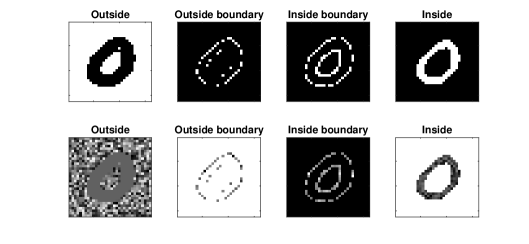
We choose CNN2 from Table 1 to classify the synthetic dataset. After CNN2 is well trained, i.e., the training error of CNN2 becomes zero, we randomly choose a synthetic image as the input of CNN2 from the testing dataset, and derive P^​(π‘­πŸ)^𝑃subscript𝑭1\hat{P}(\boldsymbol{F_{1}}), P^​(π‘­πŸ|π‘­πŸ)^𝑃conditionalsubscript𝑭2subscript𝑭1\hat{P}(\boldsymbol{F_{2}|F_{1}}), P​(π‘­πŸ‘|π‘­πŸ)𝑃conditionalsubscript𝑭3subscript𝑭2P(\boldsymbol{F_{3}|F_{2}}), and P​(𝑭𝒀|π‘­πŸ‘)𝑃conditionalsubscript𝑭𝒀subscript𝑭3P(\boldsymbol{F_{Y}|F_{3}}). Finally, all the distributions are shown in Figure 2. We can find that P^​(π‘­πŸ)^𝑃subscript𝑭1\hat{P}(\boldsymbol{F_{1}}) is indeed close to P​(𝑿)𝑃𝑿P(\boldsymbol{X}), because the KL divergence is samll, i.e., KL[P(𝑿)||P^(π‘­πŸ)]=0.49\text{KL}[P(\boldsymbol{X})||\hat{P}(\boldsymbol{F_{1}})]=0.49.

Refer to caption
Figure 2: (A) the synthetic image 𝒙𝒙\boldsymbol{x} is the input of CNN2, (B) KL[P(𝑿)||P^(𝒙)]=0.53\text{KL}[P(\boldsymbol{X})||\hat{P}(\boldsymbol{x})]=0.53, where the red curve indicates the truly prior distribution P​(𝑿)=𝒩​(0,1024)𝑃𝑿𝒩01024P(\boldsymbol{X})=\mathcal{N}(0,1024) and P^​(𝒙)^𝑃𝒙\hat{P}(\boldsymbol{x}) is the empirical distribution of 𝒙𝒙\boldsymbol{x}, (C) KL[P(𝑿)||P^(π‘­πŸ)]=0.49\text{KL}[P(\boldsymbol{X})||\hat{P}(\boldsymbol{F_{1}})]=0.49, where P^​(π‘­πŸ)^𝑃subscript𝑭1\hat{P}(\boldsymbol{F_{1}}) is the empirical distribution of π’‡πŸsubscript𝒇1\boldsymbol{f_{1}} and π’‡πŸsubscript𝒇2\boldsymbol{f_{2}}, (D) P^​(π‘­πŸ|π‘­πŸ)^𝑃conditionalsubscript𝑭2subscript𝑭1\hat{P}(\boldsymbol{F_{2}|F_{1}}) is the empirical distribution of π’‡πŸ‘subscript𝒇3\boldsymbol{f_{3}} and π’‡πŸ’subscript𝒇4\boldsymbol{f_{4}}, (E) the distribution P​(π‘­πŸ‘|π‘­πŸ)𝑃conditionalsubscript𝑭3subscript𝑭2{P}(\boldsymbol{F_{3}|F_{2}}), and (F) the distribution P​(𝑭𝒀|π‘­πŸ‘)𝑃conditionalsubscript𝑭𝒀subscript𝑭3{P}(\boldsymbol{F_{Y}|F_{3}}).

This experiment validates explicitly Bayesian regularizations in CNNs. Since we can theoretically prove CNN2 formulating a Bayesian network P​(𝑭𝒀;π‘­πŸ‘;π‘­πŸ;π‘­πŸ)𝑃subscript𝑭𝒀subscript𝑭3subscript𝑭2subscript𝑭1P(\boldsymbol{F_{Y};F_{3};F_{2};F_{1}}) and empirically show P^​(π‘­πŸ)^𝑃subscript𝑭1\hat{P}(\boldsymbol{F_{1}}) modeling the prior distribution P​(𝑿)𝑃𝑿P(\boldsymbol{X}), CNN2 has an explicitly Bayesian regularization defined by the first convolutional layer π’‡πŸsubscript𝒇1\boldsymbol{f_{1}}. In addition, the experiment validates the proposed probabilistic representation for the hidden layers of CNNs, especially the convolutional layer.

4.3 The effect of increasing the number of hidden units on the generalization performance

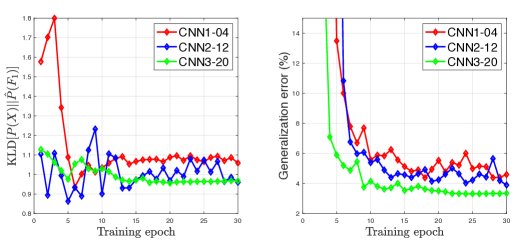
Based on the proposed Bayesian networks explanation and the experiment presented in Section 4.2, we verify that π’‡πŸsubscript𝒇1\boldsymbol{f_{1}} formulates a prior distribution as an explicit Bayesian regularization. Since the only difference within the three CNNs is that the first convolutional layer π’‡πŸsubscript𝒇1\boldsymbol{f_{1}} of different CNNs has different number of convolutional channels, we can use the three CNNs to examine the effect of increasing hidden units on the generalization performance of CNNs. We use KL[P(𝑿)||P^(π‘­πŸ)]\text{KL}[P(\boldsymbol{X})||\hat{P}(\boldsymbol{F_{1}})] to quantify the effect of increasing the number of hidden units on the prior distribution P^​(π‘­πŸ)^𝑃subscript𝑭1\hat{P}(\boldsymbol{F_{1}}), i.e., the Bayesian regularization. We average KL[P(𝑿)||P^(π‘­πŸ)]\text{KL}[P(\boldsymbol{X})||\hat{P}(\boldsymbol{F_{1}})] overall all testing images and use the testing error to quantify the generalization performance over 30 training epochs.

Figure 3 shows that increasing the number of hidden units of CNNs has a negative correlation with the generalization error, which validates the Bayesian regularization explanation (Proposition 4). Specifically, Figure 3 (Left) shows that KL[P(𝑿)||P^(π‘­πŸ)]\text{KL}[P(\boldsymbol{X})||\hat{P}(\boldsymbol{F_{1}})] is decreasing as we increase the number of hidden units. It means that π’‡πŸsubscript𝒇1\boldsymbol{f_{1}} formulates a better Bayesian regularization as increasing the number of hidden unit. As a result, the corresponding CNNs should achieve the lower generalization error, which is demonstrated by Figure 3 (Right).
Refer to caption
Figure 3: (Left) The average KL[P(𝑿)||P^(π‘­πŸ)]\text{KL}[P(\boldsymbol{X})||\hat{P}(\boldsymbol{F_{1}})] overall all testing images. (Right) The generalization performance of the three CNNs represented by the testing error. The number behind the three CNNs in the legend denotes the number of hidden units of π’‡πŸsubscript𝒇1\boldsymbol{f_{1}}.

4.4 The generalization performance of CNNs on random labels

Refer to caption
Figure 4: The distribution of the hidden layers in CNN3 given a synthetic testing image with the random label. The notation is the same as Figure 2, e.g., KL[P(𝑿)||P^(𝒙)]=0.66\text{KL}[P(\boldsymbol{X})||\hat{P}(\boldsymbol{x})]=0.66, and KL[P(𝑿)||P^(π‘­πŸ)]=0.47\text{KL}[P(\boldsymbol{X})||\hat{P}(\boldsymbol{F_{1}})]=0.47.

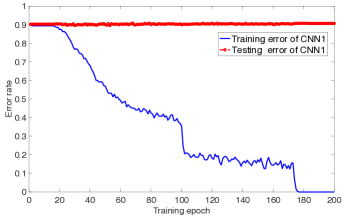
Similar to the notable experiment presented in [35], we use CNN3 to classify the synthetic dataset with random labels. Figure 5 shows CNN3 achieving zero training error but very high testing error. We visualize the distribution of hidden layers in CNN3 given a testing image with a random label, and Figure 4(C) shows that CNN3 still can learn an accurate prior distribution P^​(π‘­πŸ)^𝑃subscript𝑭1\hat{P}(\boldsymbol{F_{1}}). In this sense, CNN3 still achieves good generalization performance on random labels.

We conjecture that CNNs cannot classify random labels. In terms of Bayesian networks, CNNs describe the causality between the given dataset and the corresponding labels, which can be simplified as the joint distribution P​(𝑿,𝒀)=P​(𝒀|𝑿)​P​(𝑿)𝑃𝑿𝒀𝑃conditional𝒀𝑿𝑃𝑿P(\boldsymbol{X},\boldsymbol{Y})=P(\boldsymbol{Y|X})P(\boldsymbol{X}), where P​(𝑿)𝑃𝑿P(\boldsymbol{X}) corresponds to the prior belief, and P​(𝒀|𝑿)𝑃conditional𝒀𝑿P(\boldsymbol{Y|X}) describes the statistical causality. Leveraging their powerful representation ability, CNNs definitely can learn a P​(𝒀|𝑿)𝑃conditional𝒀𝑿P(\boldsymbol{Y|X}) from the training dataset and corresponding random labels, thus the training error is zero. However, the causality represented by the learned P​(𝒀|𝑿)𝑃conditional𝒀𝑿P(\boldsymbol{Y|X}) is obviously not consistent with the testing labels, because labels are random, thus the testing error is always around 90%percent9090\%. In summary, the high testing error on random labels is because P​(𝒀|𝑿)𝑃conditional𝒀𝑿P(\boldsymbol{Y|X}) cannot model two independent variables, but not related to the prior distribution, i.e., Bayesian regularization.
Refer to caption
Figure 5: The training and testing errors of CNN3 on random labels over 200 training epochs.

5 Conclusion

In this paper, we demonstrate CNNs have explicitly Bayesian regularizations. First, we introduce a novel probabilistic representation for the hidden layers of CNNs and demonstrate that CNNs correspond to a Bayesian network with the serial connection. We conclude that CNNs have explicitly Bayesian regularizations because the hidden layers close to the input formulate prior distributions. Moreover, based on the proposed Bayesian regularization, we clarify two recently observed empirical phenomena that are inconsistent with traditional theories of generalization. In the future, we hope to extend the proposed Bayesian regularization theory to general DNNs, e.g., the residual networks [8], and to design new regularization algorithms through pre-training the hidden layers corresponding to prior distributions for improving the generalization performance of DNNs.

References

  • [1] Sanjeev Arora, Nadav Cohen, Wei Hu, and Yuping Luo. Implicit regularization in deep matrix factorization. arXiv preprint arXiv:1905.13655, 2019.
  • [2] Roberto Battiti. First-and second-order methods for learning: between steepest descent and newton’s method. Neural computation, 4(2):141–166, 1992.
  • [3] Laurent Dinh, Razvan Pascanu, Samy Bengio, and Yoshua Bengio. Sharp minima can generalize for deep nets. In Proceedings of the 34th International Conference on Machine Learning-Volume 70, pages 1019–1028. JMLR. org, 2017.
  • [4] AdriΓ  Garriga-Alonso, CarlΒ Edward Rasmussen, and Laurence Aitchison. Deep convolutional networks as shallow gaussian processes. arXiv preprint arXiv:1808.05587, 2018.
  • [5] S.Β Geman and D.Β Geman. Stochastic relaxation, gibbs distributions, and the bayesian restoration of images. IEEE Transactions. on Pattern Analysis and Machine Intelligence, pages 721–741, June 1984.
  • [6] Ian Goodfellow, Yoshua Bengio, and Aaron Courville. Deep Learning. MIT Press, 2016.
  • [7] Suriya Gunasekar, JasonΒ D Lee, Daniel Soudry, and Nati Srebro. Implicit bias of gradient descent on linear convolutional networks. In Advances in Neural Information Processing Systems, pages 9461–9471, 2018.
  • [8] KΒ He, XΒ Zhang, SΒ Ren, and JΒ Sun. Deep residual learning for image recognition. In CVPR, pages 770–778, 2016.
  • [9] GeoffreyΒ E Hinton. Products of experts. 9th International Conference on Artificial Neural Networks, 1999.
  • [10] GeoffreyΒ E. Hinton. Training products of experts by minimizing contrastive divergence. Neural Computation, 14:1771–1800, 2002.
  • [11] NitishΒ Shirish Keskar, Dheevatsa Mudigere, Jorge Nocedal, Mikhail Smelyanskiy, and Ping TakΒ Peter Tang. On large-batch training for deep learning: Generalization gap and sharp minima. arXiv preprint arXiv:1609.04836, 2016.
  • [12] Timo Koski and John Noble. Bayesian networks: an introduction, volume 924. John Wiley & Sons, 2011.
  • [13] Krizhevsky, Sutskever A., and G.Β E. Hinton. Imagenet classification with deep convolutional neural networks. In NeurIPS, volumeΒ 25, pages 1090–1098, 2012.
  • [14] Xinjie Lan. A synthetic dataset for deep learning. arXiv preprint arXiv:1906.11905, 2019.
  • [15] Yann LeCun, Sumit Chopra, Raia Hadsell, Marc’Aurelio Ranzato, and FuΒ Jie Huang. A tutorial on energy-based learning. MIT Press, 2006.
  • [16] Jaehoon Lee, Yasaman Bahri, Roman Novak, SamuelΒ S. Schoenholz, Jeffrey Pennington, and Jascha Sohl-Dickstein. Deep neural networks as gaussian processes. In ICLR, 2018.
  • [17] Siwei Lyu and Eero.Β P. Simoncelli. Statistical modeling of images with fields of gaussian scale mixtures. In NeurIPS, 2007.
  • [18] Alexander Matthews, Mark Rowland, Jiri Hron, RichardΒ E. Turner, and Zoubin Ghahramani. Gaussian process behaviour in wide deep neural networks. In ICLR, 2018.
  • [19] Pankaj Mehta and DavidΒ J. Schwab. An exact mapping between the variational renormalization group and deep learning. arXiv preprint arXiv:1410.3831, 2014.
  • [20] Behnam Neyshabur, Srinadh Bhojanapalli, David McAllester, and Nathan Srebro. Exploring generalization in deep learning. In NeurIPS, 2017.
  • [21] Behnam Neyshabur, Ryota Tomioka, and Nathan Srebro. In search of the real inductive bias: On the role of implicit regularization in deep learning. In ICLR, 2015.
  • [22] Frank Nielsen and Vincent Garcia. Statistical exponential families: A digest with flash cards. arXiv preprint arXiv:0911.4863, 2009.
  • [23] ThomasΒ Dyhre Nielsen and FinnΒ Verner Jensen. Bayesian networks and decision graphs. Springer Science & Business Media, 2009.
  • [24] Roman Novak, Lechao Xiao, Jaehoon Lee, Yasaman Bahri, Greg Yang, Jiri Hron, DanielΒ A. Abolafia, Jeffrey Pennington, and Jascha Sohl-Dickstein. Bayesian deep convolutional networks with many channels are gaussian processes. In ICLR, 2018.
  • [25] Aaron Oord and BΒ Schrauwen. Factoring variations in natural images with deep gaussian mixture models. In NeurIPS, 2014.
  • [26] Ankit Patel, Minh Nguyen, and Richard Baraniuk. A probabilistic framework for deep learning. In NeurIPS, 2016.
  • [27] M.Β D. Richard and R.Β Lippmann. Neural network classifiers estimate bayesian a posteriori probabilities. Neural Compution, 3:461–483, 1991.
  • [28] DavidΒ E. Rumelhart, GeoffreyΒ E. Hinton, and RonaldΒ J. Williams. Learning representations by back-propagating errors. Nature, 323:533–536, October 1986.
  • [29] Ruslan Salakhutdinov and Geoffrey Hinton. Deep boltzmann machines. In AISTATS 2009, pages 448–455, 2009.
  • [30] Daniel Soudry, Elad Hoffer, MorΒ Shpigel Nacson, Suriya Gunasekar, and Nathan Srebro. The implicit bias of gradient descent on separable data. The Journal of Machine Learning Research, 19(1):2822–2878, 2018.
  • [31] Harald Steck and TommiΒ S. Jaakkola. On the dirichlet prior and bayesian regularization. In NeurIPS, 2003.
  • [32] Yichuan Tang, Ruslan Salakhutdinov, and Geoffrey Hinton. Deep mixtures of factor analysers. arXiv preprint arXiv:1206.4635, 2015.
  • [33] Chaohui Wang, Nikos Komodakis, and Nikos Paragios. Markov random field modeling, inference & learning in computer vision & image understanding: A survey. Computer Vision and Image Understanding, 117(11):1610–1627, 2013.
  • [34] Sho Yaida. Non-gaussian processes and neural networks at finite widths. arXiv preprint arXiv:1910.00019, 2019.
  • [35] Chiyuan Zhang, Samy Bengio, Moritz Hardt, Benjamin Recht, and Oriol Vinyals. Understanding deep learning requires rethinking generalization. In ICLR, 2016.
  • [36] G.Β Zhang. Neural networks for classification: a survey. IEEE Transactions on Systems, Man, and Cybernetics, 30:451–462, 2000.

6 Appendix

6.1 Proof: the proposed probabilisitic representation for the hidden layers of CNNs
Refer to caption
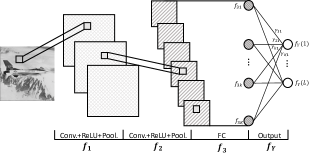
Figure 6: The CNN={𝒙;π’‡πŸ;π’‡πŸ;π’‡πŸ‘;𝒇𝒀}CNN𝒙subscript𝒇1subscript𝒇2subscript𝒇3subscript𝒇𝒀\text{CNN}=\{\boldsymbol{x;f_{1};f_{2};f_{3};f_{Y}}\} has two convolutional hidden layers π’‡πŸsubscript𝒇1\boldsymbol{f_{1}} and π’‡πŸsubscript𝒇2\boldsymbol{f_{2}} and a fully connected hidden layer π’‡πŸ‘subscript𝒇3\boldsymbol{f_{3}}. The flattening π’‡πŸsubscript𝒇2\boldsymbol{f_{2}} is the input of π’‡πŸ‘subscript𝒇3\boldsymbol{f_{3}}.

Based on the CNN show in Figure 6, we prove the proposed probabilistic representation for the hidden layers of CNNs in Section 3.2. In the above CNN, the input 𝒙𝒙\boldsymbol{x} has M𝑀M channels 𝒙={𝒙m}m=1M𝒙superscriptsubscriptsuperscriptπ’™π‘šπ‘š1𝑀\boldsymbol{x}=\{\boldsymbol{x}^{m}\}_{m=1}^{M} (e.g., M=3𝑀3M=3 if 𝒙𝒙\boldsymbol{x} are color images), π’‡πŸsubscript𝒇1\boldsymbol{f_{1}} has N𝑁N convolutional channels, i.e., π’‡πŸ={π’‡πŸπ’}n=1Nsubscript𝒇1superscriptsubscriptsuperscriptsubscript𝒇1𝒏𝑛1𝑁\boldsymbol{f_{1}}=\{\boldsymbol{f_{1}^{n}}\}_{n=1}^{N}, and π’‡πŸsubscript𝒇2\boldsymbol{f_{2}} has Q𝑄Q convolutional channels, i.e., π’‡πŸ={π’‡πŸπ’’}q=1Qsubscript𝒇2superscriptsubscriptsuperscriptsubscript𝒇2π’’π‘ž1𝑄\boldsymbol{f_{2}}=\{\boldsymbol{f_{2}^{q}}\}_{q=1}^{Q}. In addition, π’‡πŸ‘subscript𝒇3\boldsymbol{f_{3}} has K𝐾K neurons, i.e., π’‡πŸ‘={π’‡πŸ‘β€‹π’Œ}k=1Ksubscript𝒇3superscriptsubscriptsubscript𝒇3π’Œπ‘˜1𝐾\boldsymbol{f_{3}}=\{\boldsymbol{f_{3k}}\}_{k=1}^{K}.

Assuming the output layer 𝒇𝒀subscript𝒇𝒀\boldsymbol{f_{Y}} is the softmax with L𝐿L nodes, its distribution can be formulated as

P​(𝑭𝒀)={P​(fy​l)=1Z𝑭𝒀​exp​(fy​l)}l=1L𝑃subscript𝑭𝒀superscriptsubscript𝑃subscript𝑓𝑦𝑙1subscript𝑍subscript𝑭𝒀expsubscript𝑓𝑦𝑙𝑙1𝐿P(\boldsymbol{F_{Y}})=\{P(f_{yl})=\frac{1}{Z_{\boldsymbol{F_{Y}}}}\text{exp}(f_{yl})\}_{l=1}^{L} (10)

where Z𝑭𝒀=βˆ‘l=1Lexp​(fy​l)subscript𝑍subscript𝑭𝒀superscriptsubscript𝑙1𝐿expsubscript𝑓𝑦𝑙Z_{\boldsymbol{F_{Y}}}=\sum_{l=1}^{L}\text{exp}(f_{yl}) is the partition function. Since fy​l=βˆ‘k=1KΞ³k​lβ‹…f3​k+by​lsubscript𝑓𝑦𝑙superscriptsubscriptπ‘˜1𝐾⋅subscriptπ›Ύπ‘˜π‘™subscript𝑓3π‘˜subscript𝑏𝑦𝑙f_{yl}=\sum_{k=1}^{K}\gamma_{kl}\cdot f_{3k}+b_{yl}, we have

P​(𝑭𝒀)={P​(fy​l)=1Z𝒀​exp​(βˆ‘k=1KΞ³k​lβ‹…f3​k+by​l)}l=1L𝑃subscript𝑭𝒀superscriptsubscript𝑃subscript𝑓𝑦𝑙1subscript𝑍𝒀expsuperscriptsubscriptπ‘˜1𝐾⋅subscriptπ›Ύπ‘˜π‘™subscript𝑓3π‘˜subscript𝑏𝑦𝑙𝑙1𝐿P(\boldsymbol{F_{Y}})=\{P(f_{yl})=\frac{1}{Z_{\boldsymbol{Y}}}\text{exp}(\sum_{k=1}^{K}\gamma_{kl}\cdot f_{3k}+b_{yl})\}_{l=1}^{L} (11)

Based on the properties of the exponential function, i.e., exp​(a+b)=exp​(a)β‹…exp​(b)expπ‘Žπ‘β‹…expπ‘Žexp𝑏{\textstyle\text{exp}(a+b)=\text{exp}(a)\cdot\text{exp}(b)} and exp​(aβ‹…b)=[exp​(b)]aexpβ‹…π‘Žπ‘superscriptdelimited-[]expπ‘π‘Ž{\textstyle\text{exp}(a\cdot b)=[\text{exp}(b)]^{a}}, we can reformulate P​(𝑭𝒀)𝑃subscript𝑭𝒀P(\boldsymbol{F_{Y}}) as

P​(𝑭𝒀)={P​(fy​l)=1Zπ’€β€²β€‹βˆk=1K[exp​(f3​k)]Ξ³k​l}l=1L𝑃subscript𝑭𝒀superscriptsubscript𝑃subscript𝑓𝑦𝑙1subscriptsuperscript𝑍′𝒀superscriptsubscriptproductπ‘˜1𝐾superscriptdelimited-[]expsubscript𝑓3π‘˜subscriptπ›Ύπ‘˜π‘™π‘™1𝐿P(\boldsymbol{F_{Y}})=\{P(f_{yl})=\frac{1}{Z^{\prime}_{\boldsymbol{Y}}}\prod_{k=1}^{K}[\text{exp}(f_{3k})]^{\gamma_{kl}}\}_{l=1}^{L} (12)

where Z𝒀′=Z𝒀/exp​(by​l)subscriptsuperscript𝑍′𝒀subscript𝑍𝒀expsubscript𝑏𝑦𝑙Z^{\prime}_{\boldsymbol{Y}}=Z_{\boldsymbol{Y}}/\text{exp}(b_{yl}). Since {exp​(f3​k)}k=1Ksuperscriptsubscriptexpsubscript𝑓3π‘˜π‘˜1𝐾\{\text{exp}(f_{3k})\}_{k=1}^{K} are scalar, we can introduce a new partition function Zπ‘­πŸ‘=βˆ‘k=1Kexp​(f3​k)subscript𝑍subscript𝑭3superscriptsubscriptπ‘˜1𝐾expsubscript𝑓3π‘˜{\textstyle Z_{\boldsymbol{F_{3}}}=\sum_{k=1}^{K}\text{exp}(f_{3k})} such that {1Zπ‘­πŸ‘β€‹exp​(f3​k)}k=1Ksuperscriptsubscript1subscript𝑍subscript𝑭3expsubscript𝑓3π‘˜π‘˜1𝐾\{\frac{1}{Z_{\boldsymbol{F_{3}}}}\text{exp}(f_{3k})\}_{k=1}^{K} becomes a probability measure. As a result, we can further reformulate P​(𝑭𝒀)={P​(fy​l)}l=1L𝑃subscript𝑭𝒀superscriptsubscript𝑃subscript𝑓𝑦𝑙𝑙1𝐿P(\boldsymbol{F_{Y}})=\{P(f_{yl})\}_{l=1}^{L} as a Product of Expert (PoE) model as

P​(𝑭𝒀)={P​(fy​l)=1Zπ’€β€²β€²β€‹βˆk=1K[1Zπ‘­πŸ‘β€‹exp​(f3​k)]Ξ³k​l}l=1L𝑃subscript𝑭𝒀superscriptsubscript𝑃subscript𝑓𝑦𝑙1subscriptsuperscript𝑍′′𝒀superscriptsubscriptproductπ‘˜1𝐾superscriptdelimited-[]1subscript𝑍subscript𝑭3expsubscript𝑓3π‘˜subscriptπ›Ύπ‘˜π‘™π‘™1𝐿P(\boldsymbol{F_{Y}})=\{P(f_{yl})=\frac{1}{Z^{\prime\prime}_{\boldsymbol{Y}}}\prod_{k=1}^{K}[\frac{1}{Z_{\boldsymbol{F_{3}}}}\text{exp}(f_{3k})]^{\gamma_{kl}}\}_{l=1}^{L} (13)

where Z𝒀′′=Z𝒀/[exp​(by​l)β‹…βˆk=1K[Zπ‘­πŸ‘]Ξ³k​l]subscriptsuperscript𝑍′′𝒀subscript𝑍𝒀delimited-[]β‹…expsubscript𝑏𝑦𝑙superscriptsubscriptproductπ‘˜1𝐾superscriptdelimited-[]subscript𝑍subscript𝑭3subscriptπ›Ύπ‘˜π‘™{\textstyle Z^{\prime\prime}_{\boldsymbol{Y}}=Z_{\boldsymbol{Y}}/[\text{exp}(b_{yl})\cdot\prod_{k=1}^{K}[Z_{\boldsymbol{F_{3}}}]^{\gamma_{kl}}}] and each expert is defined as 1Zπ‘­πŸ‘β€‹exp​(f3​k)1subscript𝑍subscript𝑭3expsubscript𝑓3π‘˜\frac{1}{Z_{\boldsymbol{F_{3}}}}\text{exp}(f_{3k}).

It is noteworthy that all the experts {1Zπ‘­πŸ‘β€‹exp​(f3​k)}k=1Ksuperscriptsubscript1subscript𝑍subscript𝑭3expsubscript𝑓3π‘˜π‘˜1𝐾\{\frac{1}{Z_{\boldsymbol{F_{3}}}}\text{exp}(f_{3k})\}_{k=1}^{K} form a probability measure and establish an exact one-to-one correspondence to all the neurons in the third hidden layer π’‡πŸ‘subscript𝒇3\boldsymbol{f_{3}}, i.e., {f3​l}k=1Ksuperscriptsubscriptsubscript𝑓3π‘™π‘˜1𝐾\{f_{3l}\}_{k=1}^{K}. Therefore, the distribution of π’‡πŸ‘subscript𝒇3\boldsymbol{f_{3}} can be expressed as

P​(π‘­πŸ‘)={P​(f3​k)=1Zπ‘­πŸ‘β€‹exp​(f3​k)}k=1K𝑃subscript𝑭3superscriptsubscript𝑃subscript𝑓3π‘˜1subscript𝑍subscript𝑭3expsubscript𝑓3π‘˜π‘˜1𝐾P(\boldsymbol{F_{3}})=\{P(f_{3k})=\frac{1}{Z_{\boldsymbol{F_{3}}}}\text{exp}(f_{3k})\}_{k=1}^{K} (14)

Based on the definition of Boltzmann distribution, Equation 10 and 14 show that 𝒇𝒀subscript𝒇𝒀\boldsymbol{f_{Y}} and π’‡πŸ‘subscript𝒇3\boldsymbol{f_{3}} formulate two multivariate Boltzmann distributions and their energy functions are equivalent to the negative of the output nodes {fy​l}l=1Lsuperscriptsubscriptsubscript𝑓𝑦𝑙𝑙1𝐿\{f_{yl}\}_{l=1}^{L} and the neurons {f3​k}k=1Ksuperscriptsubscriptsubscript𝑓3π‘˜π‘˜1𝐾\{f_{3k}\}_{k=1}^{K}, respectively.

In summary, the above derivation proves Proposition 1, i.e., a fully connected layer formulates a multivariate discrete Boltzmann distribution and the energy function of which is equivalent to the negative activations of the fully connected layer. The subsequent derivation proves Proposition 2.

Since {f3​k=βˆ‘j=1JΞ²j​kβ‹…f2​j+b3​k}k=1Ksuperscriptsubscriptsubscript𝑓3π‘˜superscriptsubscript𝑗1𝐽⋅subscriptπ›½π‘—π‘˜subscript𝑓2𝑗subscript𝑏3π‘˜π‘˜1𝐾\{f_{3k}=\sum_{j=1}^{J}\beta_{jk}\cdot f_{2j}+b_{3k}\}_{k=1}^{K}, we can derive

P​(π‘­πŸ‘)={P​(f3​k)=1Zπ‘­πŸ‘β€‹exp​(βˆ‘j=1JΞ²j​kβ‹…f2​j+b3​k)}k=1K𝑃subscript𝑭3superscriptsubscript𝑃subscript𝑓3π‘˜1subscript𝑍subscript𝑭3expsuperscriptsubscript𝑗1𝐽⋅subscriptπ›½π‘—π‘˜subscript𝑓2𝑗subscript𝑏3π‘˜π‘˜1𝐾P(\boldsymbol{F_{3}})=\{P(f_{3k})=\frac{1}{Z_{\boldsymbol{F_{3}}}}\text{exp}(\sum_{j=1}^{J}\beta_{jk}\cdot f_{2j}+b_{3k})\}_{k=1}^{K} (15)

where {f2​j}j=1Jsuperscriptsubscriptsubscript𝑓2𝑗𝑗1𝐽\{f_{2j}\}_{j=1}^{J} is the flattened output of π’‡πŸsubscript𝒇2\boldsymbol{f_{2}}, Ξ²j​ksubscriptπ›½π‘—π‘˜\beta_{jk} is the weight of the edge between f2​jsubscript𝑓2𝑗f_{2j} and f3​ksubscript𝑓3π‘˜f_{3k}, and b3​ksubscript𝑏3π‘˜b_{3k} denotes the bias. Since π’‡πŸsubscript𝒇2\boldsymbol{f_{2}} is a convolutional layer with Q𝑄Q convolutional channels, it can be reformulated as {f2​j}j=1J={π’‡πŸπ’’}q=1Qsuperscriptsubscriptsubscript𝑓2𝑗𝑗1𝐽superscriptsubscriptsubscriptsuperscript𝒇𝒒2π‘ž1𝑄\{f_{2j}\}_{j=1}^{J}=\{\boldsymbol{f^{q}_{2}}\}_{q=1}^{Q}. As a result, P​(π‘­πŸ‘)𝑃subscript𝑭3P(\boldsymbol{F_{3}}) can be reformulated as

P​(π‘­πŸ‘)={P​(f3​k)=1Zπ‘­πŸ‘β€‹exp​(βˆ‘q=1Q𝜷q​kTβ‹…π’‡πŸπ’’+b3​k)}k=1K𝑃subscript𝑭3superscriptsubscript𝑃subscript𝑓3π‘˜1subscript𝑍subscript𝑭3expsuperscriptsubscriptπ‘ž1𝑄⋅subscriptsuperscriptπœ·π‘‡π‘žπ‘˜subscriptsuperscript𝒇𝒒2subscript𝑏3π‘˜π‘˜1𝐾P(\boldsymbol{F_{3}})=\{P(f_{3k})=\frac{1}{Z_{\boldsymbol{F_{3}}}}\text{exp}(\sum_{q=1}^{Q}\boldsymbol{\beta}^{T}_{qk}\cdot\boldsymbol{f^{q}_{2}}+b_{3k})\}_{k=1}^{K} (16)

where 𝜷q​ksubscriptπœ·π‘žπ‘˜\boldsymbol{\beta}_{qk} is a subset of the parameters {Ξ²j​k}j=1Jsuperscriptsubscriptsubscriptπ›½π‘—π‘˜π‘—1𝐽\{\beta_{jk}\}_{j=1}^{J} such that βˆ‘q=1Q𝜷q​kT⋅𝒇2q=βˆ‘j=1JΞ²j​kβ‹…f2​jsuperscriptsubscriptπ‘ž1𝑄⋅subscriptsuperscriptπœ·π‘‡π‘žπ‘˜subscriptsuperscriptπ’‡π‘ž2superscriptsubscript𝑗1𝐽⋅subscriptπ›½π‘—π‘˜subscript𝑓2𝑗\sum_{q=1}^{Q}\boldsymbol{\beta}^{T}_{qk}\cdot\boldsymbol{f}^{q}_{2}=\sum_{j=1}^{J}\beta_{jk}\cdot f_{2j}, and 𝜷q​kTsubscriptsuperscriptπœ·π‘‡π‘žπ‘˜\boldsymbol{\beta}^{T}_{qk} is the transpose of 𝜷q​ksubscriptπœ·π‘žπ‘˜\boldsymbol{\beta}_{qk}. Therefore, P​(π‘­πŸ‘)𝑃subscript𝑭3P(\boldsymbol{F_{3}}) can be reformulated as

P​(π‘­πŸ‘)={P​(f3​k)=1Zπ‘­πŸ‘β€²β€‹βˆq=1Qexp​(𝜷q​kTβ‹…π’‡πŸπ’’)}k=1K𝑃subscript𝑭3superscriptsubscript𝑃subscript𝑓3π‘˜1subscriptsuperscript𝑍′subscript𝑭3superscriptsubscriptproductπ‘ž1𝑄expβ‹…subscriptsuperscriptπœ·π‘‡π‘žπ‘˜subscriptsuperscript𝒇𝒒2π‘˜1𝐾P(\boldsymbol{F_{3}})=\{P(f_{3k})=\frac{1}{Z^{\prime}_{\boldsymbol{F_{3}}}}\prod_{q=1}^{Q}\text{exp}(\boldsymbol{\beta}^{T}_{qk}\cdot\boldsymbol{f^{q}_{2}})\}_{k=1}^{K} (17)

where Zπ‘­πŸ‘β€²=Zπ‘­πŸ‘/[exp​(b3​k)]subscriptsuperscript𝑍′subscript𝑭3subscript𝑍subscript𝑭3delimited-[]expsubscript𝑏3π‘˜Z^{\prime}_{\boldsymbol{F_{3}}}=Z_{\boldsymbol{F_{3}}}/[\text{exp}(b_{3k})]. Recall the element-wise matrix power, e.g., exp​(𝒂)𝒃expsuperscript𝒂𝒃\text{exp}(\boldsymbol{a})^{\boldsymbol{b}}, where 𝒂=[a1;a2;a3]𝒂subscriptπ‘Ž1subscriptπ‘Ž2subscriptπ‘Ž3\boldsymbol{a}=[a_{1};a_{2};a_{3}] and 𝒃=[b1;b2;b3]𝒃subscript𝑏1subscript𝑏2subscript𝑏3\boldsymbol{b}=[b_{1};b_{2};b_{3}], we can derive that exp​(𝒂)=[exp​(a1);exp​(a2);exp​(a3)]exp𝒂expsubscriptπ‘Ž1expsubscriptπ‘Ž2expsubscriptπ‘Ž3\text{exp}(\boldsymbol{a})=[\text{exp}(a_{1});\text{exp}(a_{2});\text{exp}(a_{3})] and exp​(𝒂)𝒃=[exp​(a1)b1;exp​(a2)b2;exp​(a3)b3]=[exp​(a1​b1);exp​(a2​b2);exp​(a3​b3)]expsuperscript𝒂𝒃expsuperscriptsubscriptπ‘Ž1subscript𝑏1expsuperscriptsubscriptπ‘Ž2subscript𝑏2expsuperscriptsubscriptπ‘Ž3subscript𝑏3expsubscriptπ‘Ž1subscript𝑏1expsubscriptπ‘Ž2subscript𝑏2expsubscriptπ‘Ž3subscript𝑏3\text{exp}(\boldsymbol{a})^{\boldsymbol{b}}=[\text{exp}(a_{1})^{b_{1}};\text{exp}(a_{2})^{b_{2}};\text{exp}(a_{3})^{b_{3}}]=[\text{exp}(a_{1}b_{1});\text{exp}(a_{2}b_{2});\text{exp}(a_{3}b_{3})]. As a result, exp​(𝒂​𝒃)=exp​(a1​b1+a2​b2+a3​b3)=∏|a|exp​(𝒂)𝒃exp𝒂𝒃expsubscriptπ‘Ž1subscript𝑏1subscriptπ‘Ž2subscript𝑏2subscriptπ‘Ž3subscript𝑏3subscriptproductπ‘Žexpsuperscript𝒂𝒃\text{exp}(\boldsymbol{ab})=\text{exp}(a_{1}b_{1}+a_{2}b_{2}+a_{3}b_{3})=\prod_{|a|}\text{exp}(\boldsymbol{a})^{\boldsymbol{b}}, where |𝒂|𝒂|\boldsymbol{a}| is the number of elements in 𝒂𝒂\boldsymbol{a}.

Based on the element-wise matrix power, we can reformulate P​(π‘­πŸ‘)𝑃subscript𝑭3P(\boldsymbol{F_{3}}) as

P​(π‘­πŸ‘)={P​(f3​k)β‰ˆ1Zπ‘­πŸ‘β€²β€‹βˆq=1Qexp​(𝜷q​kTβ‹…π’‡πŸπ’’)=1Zπ‘­πŸ‘β€²β€‹βˆq=1Q∏|π’‡πŸπ’’|[exp​(π’‡πŸπ’’)]𝜷q​k}k=1K𝑃subscript𝑭3superscriptsubscript𝑃subscript𝑓3π‘˜1subscriptsuperscript𝑍′subscript𝑭3superscriptsubscriptproductπ‘ž1𝑄expβ‹…subscriptsuperscriptπœ·π‘‡π‘žπ‘˜subscriptsuperscript𝒇𝒒21subscriptsuperscript𝑍′subscript𝑭3superscriptsubscriptproductπ‘ž1𝑄subscriptproductsubscriptsuperscript𝒇𝒒2superscriptdelimited-[]expsubscriptsuperscript𝒇𝒒2subscriptπœ·π‘žπ‘˜π‘˜1𝐾P(\boldsymbol{F_{3}})=\{P(f_{3k})\approx\frac{1}{Z^{\prime}_{\boldsymbol{F_{3}}}}\prod_{q=1}^{Q}\text{exp}(\boldsymbol{\beta}^{T}_{qk}\cdot\boldsymbol{f^{q}_{2}})=\frac{1}{Z^{\prime}_{\boldsymbol{F_{3}}}}\prod_{q=1}^{Q}\prod_{|\boldsymbol{f^{q}_{2}}|}[\text{exp}(\boldsymbol{f^{q}_{2}})]^{\boldsymbol{\beta}_{qk}}\}_{k=1}^{K} (18)

Moreover, we introduce a new partition function Zπ‘­πŸπ’’=βˆ‘π’‡πŸπ’’exp​(π’‡πŸπ’’)subscript𝑍subscriptsuperscript𝑭𝒒2subscriptsubscriptsuperscript𝒇𝒒2expsubscriptsuperscript𝒇𝒒2Z_{\boldsymbol{F^{q}_{2}}}=\sum_{\boldsymbol{f^{q}_{2}}}\text{exp}(\boldsymbol{f^{q}_{2}}) to guarantee that 1Zπ‘­πŸπ’’β€‹exp​(π’‡πŸπ’’)1subscript𝑍subscriptsuperscript𝑭𝒒2expsubscriptsuperscript𝒇𝒒2\frac{1}{Z_{\boldsymbol{F^{q}_{2}}}}\text{exp}(\boldsymbol{f^{q}_{2}}) is a probability measure. As a result, P​(π‘­πŸ‘)𝑃subscript𝑭3P(\boldsymbol{F_{3}}) can be reformulated as

P​(π‘­πŸ‘)={P​(f3​k)=1Zπ‘­πŸ‘β€²β€²β€‹βˆq=1Q∏|π’‡πŸπ’’|[1Zπ‘­πŸπ’’β€‹exp​(π’‡πŸπ’’)]𝜷q​k}k=1K𝑃subscript𝑭3superscriptsubscript𝑃subscript𝑓3π‘˜1subscriptsuperscript𝑍′′subscript𝑭3superscriptsubscriptproductπ‘ž1𝑄subscriptproductsubscriptsuperscript𝒇𝒒2superscriptdelimited-[]1subscript𝑍subscriptsuperscript𝑭𝒒2expsubscriptsuperscript𝒇𝒒2subscriptπœ·π‘žπ‘˜π‘˜1𝐾P(\boldsymbol{F_{3}})=\{P(f_{3k})=\frac{1}{Z^{\prime\prime}_{\boldsymbol{F_{3}}}}\prod_{q=1}^{Q}\prod_{|\boldsymbol{f^{q}_{2}}|}[\frac{1}{Z_{\boldsymbol{F^{q}_{2}}}}\text{exp}(\boldsymbol{f^{q}_{2}})]^{\boldsymbol{\beta}_{qk}}\}_{k=1}^{K} (19)

where Zπ‘­πŸ‘β€²β€²=Zπ‘­πŸ‘β€²/∏q=1Q[Zπ‘­πŸπ’’]𝜷q​kβ‹…|π’‡πŸπ’’|subscriptsuperscript𝑍′′subscript𝑭3subscriptsuperscript𝑍′subscript𝑭3superscriptsubscriptproductπ‘ž1𝑄superscriptdelimited-[]subscript𝑍subscriptsuperscript𝑭𝒒2β‹…subscriptπœ·π‘žπ‘˜subscriptsuperscript𝒇𝒒2Z^{\prime\prime}_{\boldsymbol{F_{3}}}=Z^{\prime}_{\boldsymbol{F_{3}}}/\prod_{q=1}^{Q}[Z_{\boldsymbol{F^{q}_{2}}}]^{\boldsymbol{\beta}_{qk}\cdot|\boldsymbol{f^{q}_{2}}|}. Overall, P​(π‘­πŸ‘)𝑃subscript𝑭3P(\boldsymbol{F_{3}}) can be reformulated as a PoE model, in which each expert is defined by every convolutional channel in π’‡πŸsubscript𝒇2\boldsymbol{f_{2}}

P​(𝒇2q)=1Zπ‘­πŸπ’’β€‹exp​(π’‡πŸπ’’)𝑃subscriptsuperscriptπ’‡π‘ž21subscript𝑍subscriptsuperscript𝑭𝒒2expsubscriptsuperscript𝒇𝒒2P(\boldsymbol{f}^{q}_{2})=\frac{1}{Z_{\boldsymbol{F^{q}_{2}}}}\text{exp}(\boldsymbol{f^{q}_{2}}) (20)

Since π’‡πŸsubscript𝒇2\boldsymbol{f_{2}} has K𝐾K convolutional channels, i.e., π’‡πŸ={π’‡πŸπ’’}q=1Qsubscript𝒇2superscriptsubscriptsubscriptsuperscript𝒇𝒒2π‘ž1𝑄\boldsymbol{f_{2}}=\{\boldsymbol{f^{q}_{2}}\}_{q=1}^{Q}, and each channel can be formulated as the summation of all the convolutional channels in π’‡πŸsubscript𝒇1\boldsymbol{f_{1}}, i.e.,

π’‡πŸ={π’‡πŸπ’’=Οƒ2​(βˆ‘n=1Nπ‘ΊπŸ(𝒒,𝒏)βˆ˜π’‡πŸπ’+b2qβ‹…πŸ)}q=1Qsubscript𝒇2superscriptsubscriptsubscriptsuperscript𝒇𝒒2subscript𝜎2superscriptsubscript𝑛1𝑁subscriptsuperscript𝑺𝒒𝒏2subscriptsuperscript𝒇𝒏1β‹…subscriptsuperscriptπ‘π‘ž21π‘ž1𝑄\boldsymbol{f_{2}}=\{\boldsymbol{f^{q}_{2}}=\sigma_{2}(\sum_{n=1}^{N}\boldsymbol{S^{(q,n)}_{2}}\circ\boldsymbol{f^{n}_{1}}+b^{q}_{2}\cdot\boldsymbol{1})\}_{q=1}^{Q} (21)

where π‘ΊπŸ(𝒒,𝒏)βˆ˜π’‡πŸπ’subscriptsuperscript𝑺𝒒𝒏2subscriptsuperscript𝒇𝒏1\boldsymbol{S^{(q,n)}_{2}}\circ\boldsymbol{f^{n}_{1}} is the output of the qπ‘žqth convolutional filter applying into the n𝑛nth channel of π’‡πŸsubscript𝒇1\boldsymbol{f_{1}}, b2qsuperscriptsubscript𝑏2π‘žb_{2}^{q} is the bias, and Οƒ2​(β‹…)subscript𝜎2β‹…\sigma_{2}(\cdot) is the activation function. Therefore, we have

P​(𝒇2q)=1Zπ‘­πŸπ’’β€‹exp​[Οƒ2​(βˆ‘n=1Nπ‘ΊπŸ(𝒒,𝒏)βˆ˜π’‡πŸπ’+b2qβ‹…πŸ)]𝑃subscriptsuperscriptπ’‡π‘ž21subscript𝑍subscriptsuperscript𝑭𝒒2expdelimited-[]subscript𝜎2superscriptsubscript𝑛1𝑁subscriptsuperscript𝑺𝒒𝒏2subscriptsuperscript𝒇𝒏1β‹…subscriptsuperscriptπ‘π‘ž21P(\boldsymbol{f}^{q}_{2})=\frac{1}{Z_{\boldsymbol{F^{q}_{2}}}}\text{exp}[\sigma_{2}(\sum_{n=1}^{N}\boldsymbol{S^{(q,n)}_{2}}\circ\boldsymbol{f^{n}_{1}}+b^{q}_{2}\cdot\boldsymbol{1})] (22)

Based on the equivalence between the gradient descent learning and the first order approximation (Appendix 6.4), Equation 22 can be approximated as

P​(𝒇2q)β‰ˆ1Zπ‘­πŸπ’’β€‹exp​(βˆ‘n=1Nπ‘ΊπŸ(𝒒,𝒏)βˆ˜π’‡πŸπ’+b2qβ‹…πŸ)𝑃subscriptsuperscriptπ’‡π‘ž21subscript𝑍subscriptsuperscript𝑭𝒒2expsuperscriptsubscript𝑛1𝑁subscriptsuperscript𝑺𝒒𝒏2subscriptsuperscript𝒇𝒏1β‹…subscriptsuperscriptπ‘π‘ž21P(\boldsymbol{f}^{q}_{2})\approx\frac{1}{Z_{\boldsymbol{F^{q}_{2}}}}\text{exp}(\sum_{n=1}^{N}\boldsymbol{S^{(q,n)}_{2}}\circ\boldsymbol{f^{n}_{1}}+b^{q}_{2}\cdot\boldsymbol{1}) (23)

Let us define a linear function as Ο†2q​(π’‡πŸ)=βˆ‘n=1Nπ‘ΊπŸ(𝒒,𝒏)βˆ˜π’‡πŸπ’+b2qβ‹…πŸsubscriptsuperscriptπœ‘π‘ž2subscript𝒇1superscriptsubscript𝑛1𝑁subscriptsuperscript𝑺𝒒𝒏2subscriptsuperscript𝒇𝒏1β‹…subscriptsuperscriptπ‘π‘ž21\varphi^{q}_{2}(\boldsymbol{f_{1}})=\sum_{n=1}^{N}\boldsymbol{S^{(q,n)}_{2}}\circ\boldsymbol{f^{n}_{1}}+b^{q}_{2}\cdot\boldsymbol{1}, thus the distribution of the qπ‘žqth convolutional channel in π’‡πŸsubscript𝒇2\boldsymbol{f_{2}}, i.e., P​(𝒇2q)𝑃subscriptsuperscriptπ’‡π‘ž2P(\boldsymbol{f}^{q}_{2}), can be expressed as

P​(𝒇2q)β‰ˆ1Zπ‘­πŸπ’’β€‹exp​[Ο†2q​(π’‡πŸ)]𝑃subscriptsuperscriptπ’‡π‘ž21subscript𝑍subscriptsuperscript𝑭𝒒2expdelimited-[]subscriptsuperscriptπœ‘π‘ž2subscript𝒇1P(\boldsymbol{f}^{q}_{2})\approx\frac{1}{Z_{\boldsymbol{F^{q}_{2}}}}\text{exp}[\varphi^{q}_{2}(\boldsymbol{f_{1}})] (24)

If we regard all the linear filters {Ο†2q​(π’‡πŸ)}k=1Ksuperscriptsubscriptsubscriptsuperscriptπœ‘π‘ž2subscript𝒇1π‘˜1𝐾\{\varphi^{q}_{2}(\boldsymbol{f_{1}})\}_{k=1}^{K} as potential functions for modeling signal structures of π’‡πŸsubscript𝒇1\boldsymbol{f_{1}}, we can formulate P​(π‘­πŸ)𝑃subscript𝑭2P(\boldsymbol{F_{2}}) as a specific Boltzmann distribution, i.e., the Markov Random Fields (MRFs), which can be expressed as

P​(π‘­πŸ)=1Zπ‘­πŸβ€‹βˆq=1QP​(𝒇2q)=1Zπ‘­πŸβ€‹exp​[βˆ‘q=1QΟ†2q​(π’‡πŸ)]𝑃subscript𝑭21subscript𝑍subscript𝑭2superscriptsubscriptproductπ‘ž1𝑄𝑃subscriptsuperscriptπ’‡π‘ž21subscript𝑍subscript𝑭2expdelimited-[]superscriptsubscriptπ‘ž1𝑄subscriptsuperscriptπœ‘π‘ž2subscript𝒇1P(\boldsymbol{F_{2}})=\frac{1}{Z_{\boldsymbol{F_{2}}}}\prod_{q=1}^{Q}P(\boldsymbol{f}^{q}_{2})=\frac{1}{Z_{\boldsymbol{F_{2}}}}\text{exp}[\sum_{q=1}^{Q}\varphi^{q}_{2}(\boldsymbol{f_{1}})] (25)

where Zπ‘­πŸ=βˆ«π’‡πŸexp​[βˆ‘q=1QΟ†2k​(π’‡πŸ)]β€‹π‘‘π’‡πŸsubscript𝑍subscript𝑭2subscriptsubscript𝒇1expdelimited-[]superscriptsubscriptπ‘ž1𝑄subscriptsuperscriptπœ‘π‘˜2subscript𝒇1differential-dsubscript𝒇1Z_{\boldsymbol{F_{2}}}=\int_{\boldsymbol{f_{1}}}\text{exp}[\sum_{q=1}^{Q}\varphi^{k}_{2}(\boldsymbol{f_{1}})]d\boldsymbol{f_{1}} is the partition function for P​(π‘­πŸ)𝑃subscript𝑭2P(\boldsymbol{F_{2}}). In summary, we prove that the convolutional layer π’‡πŸsubscript𝒇2\boldsymbol{f_{2}} formulates a MRF model to describe the statistical property of π’‡πŸsubscript𝒇1\boldsymbol{f_{1}}.

Refer to caption
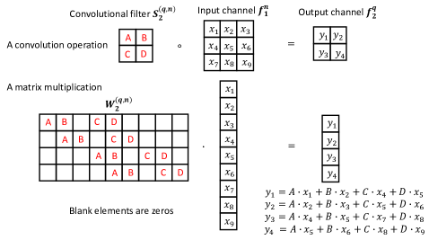
Figure 7: The equivalence between a convolutional operation and a matrix multiplication.

Subsequently, we prove that the convolutional layer π’‡πŸsubscript𝒇1\boldsymbol{f_{1}} also formulates a MRF model to describe the statistical property of the input 𝒙𝒙\boldsymbol{x}. Based on Equation 23, we have

P​(𝒇2q)β‰ˆ1Zπ‘­πŸπ’’β€²β€‹exp​(βˆ‘n=1Nπ‘ΊπŸ(𝒒,𝒏)βˆ˜π’‡πŸπ’)𝑃subscriptsuperscriptπ’‡π‘ž21subscriptsuperscript𝑍′subscriptsuperscript𝑭𝒒2expsuperscriptsubscript𝑛1𝑁subscriptsuperscript𝑺𝒒𝒏2subscriptsuperscript𝒇𝒏1P(\boldsymbol{f}^{q}_{2})\approx\frac{1}{Z^{\prime}_{\boldsymbol{F^{q}_{2}}}}\text{exp}(\sum_{n=1}^{N}\boldsymbol{S^{(q,n)}_{2}}\circ\boldsymbol{f^{n}_{1}}) (26)

where Zπ‘­πŸπ’Œβ€²=Zπ‘­πŸπ’’/exp​(b2q)subscriptsuperscript𝑍′subscriptsuperscriptπ‘­π’Œ2subscript𝑍subscriptsuperscript𝑭𝒒2expsubscriptsuperscriptπ‘π‘ž2Z^{\prime}_{\boldsymbol{F^{k}_{2}}}=Z_{\boldsymbol{F^{q}_{2}}}/\text{exp}(b^{q}_{2}). Based on the equivalence between a convolutional channel and a matrix multiplication proven in Appendix 6.5, we can regard a convolutional operation as a matrix multiplication, which is visualized in Figure 7. As a result, we have

P​(𝒇2q)β‰ˆ1Zπ‘­πŸπ’’β€²β€‹exp​(βˆ‘n=1Nπ‘ΊπŸ(𝒒,𝒏)βˆ˜π’‡πŸπ’)=1Zπ‘­πŸπ’’β€²β€‹exp​(βˆ‘n=1Nπ‘ΎπŸ(𝒒,𝒏)β‹…π’‡πŸπ’)𝑃subscriptsuperscriptπ’‡π‘ž21subscriptsuperscript𝑍′subscriptsuperscript𝑭𝒒2expsuperscriptsubscript𝑛1𝑁subscriptsuperscript𝑺𝒒𝒏2subscriptsuperscript𝒇𝒏11subscriptsuperscript𝑍′subscriptsuperscript𝑭𝒒2expsuperscriptsubscript𝑛1𝑁⋅subscriptsuperscript𝑾𝒒𝒏2subscriptsuperscript𝒇𝒏1P(\boldsymbol{f}^{q}_{2})\approx\frac{1}{Z^{\prime}_{\boldsymbol{F^{q}_{2}}}}\text{exp}(\sum_{n=1}^{N}\boldsymbol{S^{(q,n)}_{2}}\circ\boldsymbol{f^{n}_{1}})=\frac{1}{Z^{\prime}_{\boldsymbol{F^{q}_{2}}}}\text{exp}(\sum_{n=1}^{N}\boldsymbol{W^{(q,n)}_{2}}\cdot\boldsymbol{f^{n}_{1}}) (27)

where π‘ΎπŸ(𝒒,𝒏)subscriptsuperscript𝑾𝒒𝒏2\boldsymbol{W^{(q,n)}_{2}} is a matrix corresponding to the convolution filter π‘ΊπŸ(𝒒,𝒏)subscriptsuperscript𝑺𝒒𝒏2\boldsymbol{S^{(q,n)}_{2}}.

Based on the element-wise matrix power, P​(𝒇2q)𝑃subscriptsuperscriptπ’‡π‘ž2P(\boldsymbol{f}^{q}_{2}) can be reformulated as

P​(𝒇2q)β‰ˆ1Zπ‘­πŸπ’’β€²β€‹βˆn=1Nexp​(π‘ΎπŸ(𝒒,𝒏)β‹…π’‡πŸπ’)=1Zπ‘­πŸπ’’β€²β€‹βˆn=1Nexp​(π’‡πŸπ’)π‘ΎπŸ(𝒒,𝒏)𝑃subscriptsuperscriptπ’‡π‘ž21subscriptsuperscript𝑍′subscriptsuperscript𝑭𝒒2superscriptsubscriptproduct𝑛1𝑁expβ‹…subscriptsuperscript𝑾𝒒𝒏2subscriptsuperscript𝒇𝒏11subscriptsuperscript𝑍′subscriptsuperscript𝑭𝒒2superscriptsubscriptproduct𝑛1𝑁expsuperscriptsubscriptsuperscript𝒇𝒏1subscriptsuperscript𝑾𝒒𝒏2P(\boldsymbol{f}^{q}_{2})\approx\frac{1}{Z^{\prime}_{\boldsymbol{F^{q}_{2}}}}\prod_{n=1}^{N}\text{exp}(\boldsymbol{W^{(q,n)}_{2}}\cdot\boldsymbol{f^{n}_{1}})=\frac{1}{Z^{\prime}_{\boldsymbol{F^{q}_{2}}}}\prod_{n=1}^{N}\text{exp}(\boldsymbol{f^{n}_{1}})^{\boldsymbol{W^{(q,n)}_{2}}} (28)

Similarly, we introduce a new partition function Zπ‘­πŸπ’=βˆ«π’‡πŸπ’exp​(π’‡πŸπ’)β€‹π‘‘π’‡πŸπ’subscript𝑍subscriptsuperscript𝑭𝒏1subscriptsubscriptsuperscript𝒇𝒏1expsubscriptsuperscript𝒇𝒏1differential-dsubscriptsuperscript𝒇𝒏1Z_{\boldsymbol{F^{n}_{1}}}=\int_{\boldsymbol{f^{n}_{1}}}\text{exp}(\boldsymbol{f^{n}_{1}})d\boldsymbol{f^{n}_{1}} to guarantee that 1Zπ‘­πŸπ’β€‹exp​(π’‡πŸπ’)1subscript𝑍subscriptsuperscript𝑭𝒏1expsubscriptsuperscript𝒇𝒏1\frac{1}{Z_{\boldsymbol{F^{n}_{1}}}}\text{exp}(\boldsymbol{f^{n}_{1}}) is a probability measure. As a result, P​(π’‡πŸπ’’)𝑃subscriptsuperscript𝒇𝒒2P(\boldsymbol{f^{q}_{2}}) can be reformulated as

P​(π’‡πŸπ’’)=P​(fy​l)β‰ˆ1Zπ‘­πŸπ’’β€²β€²β€‹βˆn=1N[1Zπ‘­πŸπ’β€‹exp​(π’‡πŸπ’)]π‘ΎπŸ(𝒒,𝒏)𝑃subscriptsuperscript𝒇𝒒2𝑃subscript𝑓𝑦𝑙1subscriptsuperscript𝑍′′subscriptsuperscript𝑭𝒒2superscriptsubscriptproduct𝑛1𝑁superscriptdelimited-[]1subscript𝑍subscriptsuperscript𝑭𝒏1expsubscriptsuperscript𝒇𝒏1subscriptsuperscript𝑾𝒒𝒏2P(\boldsymbol{f^{q}_{2}})=P(f_{yl})\approx\frac{1}{Z^{\prime\prime}_{\boldsymbol{F^{q}_{2}}}}\prod_{n=1}^{N}[\frac{1}{Z_{\boldsymbol{F^{n}_{1}}}}\text{exp}(\boldsymbol{f^{n}_{1}})]^{\boldsymbol{W^{(q,n)}_{2}}} (29)

where Zπ‘­πŸπ’’β€²β€²=Zπ‘­πŸπ’’β€²/∏n=1N[Zπ‘­πŸπ’]π‘ΎπŸ(𝒒,𝒏)subscriptsuperscript𝑍′′subscriptsuperscript𝑭𝒒2subscriptsuperscript𝑍′subscriptsuperscript𝑭𝒒2superscriptsubscriptproduct𝑛1𝑁superscriptdelimited-[]subscript𝑍subscriptsuperscript𝑭𝒏1subscriptsuperscript𝑾𝒒𝒏2Z^{\prime\prime}_{\boldsymbol{F^{q}_{2}}}=Z^{\prime}_{\boldsymbol{F^{q}_{2}}}/\prod_{n=1}^{N}[Z_{\boldsymbol{F^{n}_{1}}}]^{\boldsymbol{W^{(q,n)}_{2}}}. Therefore, P​(π’‡πŸπ’’)𝑃subscriptsuperscript𝒇𝒒2P(\boldsymbol{f^{q}_{2}}) can be reformulated as a PoE model, in which all the experts are defined as P​(π’‡πŸπ’)=1Zπ‘­πŸπ’β€‹exp​(π’‡πŸπ’)𝑃subscriptsuperscript𝒇𝒏11subscript𝑍subscriptsuperscript𝑭𝒏1expsubscriptsuperscript𝒇𝒏1P(\boldsymbol{f^{n}_{1}})=\frac{1}{Z_{\boldsymbol{F^{n}_{1}}}}\text{exp}(\boldsymbol{f^{n}_{1}}).

Since π’‡πŸsubscript𝒇1\boldsymbol{f_{1}} has N𝑁N convolutional channels

π’‡πŸ={π’‡πŸπ’=Οƒ1​(βˆ‘m=1Mπ‘ΊπŸ(𝒏,π’Ž)βˆ˜π’™π’Ž+b1nβ‹…πŸ)}n=1Nsubscript𝒇1superscriptsubscriptsubscriptsuperscript𝒇𝒏1subscript𝜎1superscriptsubscriptπ‘š1𝑀subscriptsuperscriptπ‘Ίπ’π’Ž1superscriptπ’™π’Žβ‹…subscriptsuperscript𝑏𝑛11𝑛1𝑁\boldsymbol{f_{1}}=\{\boldsymbol{f^{n}_{1}}=\sigma_{1}(\sum_{m=1}^{M}\boldsymbol{S^{(n,m)}_{1}}\circ\boldsymbol{x^{m}}+b^{n}_{1}\cdot\boldsymbol{1})\}_{n=1}^{N} (30)

Based on the same derivation as Equations 23, 24, 25, P​(π‘­πŸ)𝑃subscript𝑭1P(\boldsymbol{F_{1}}) also can be expressed as a MRF model

P​(π‘­πŸ)=1Zπ‘­πŸβ€‹βˆn=1NP​(𝒇1n)=1Zπ‘­πŸβ€‹exp​[βˆ‘n=1NΟ†1n​(𝒙)]𝑃subscript𝑭11subscript𝑍subscript𝑭1superscriptsubscriptproduct𝑛1𝑁𝑃subscriptsuperscript𝒇𝑛11subscript𝑍subscript𝑭1expdelimited-[]superscriptsubscript𝑛1𝑁subscriptsuperscriptπœ‘π‘›1𝒙P(\boldsymbol{F_{1}})=\frac{1}{Z_{\boldsymbol{F_{1}}}}\prod_{n=1}^{N}P(\boldsymbol{f}^{n}_{1})=\frac{1}{Z_{\boldsymbol{F_{1}}}}\text{exp}[\sum_{n=1}^{N}\varphi^{n}_{1}(\boldsymbol{x})] (31)

where Ο†1n(𝒙)=βˆ‘m=1Mπ‘ΊπŸ(𝒏,π’Ž)βˆ˜π’™π’Ž+b1nβ‹…πŸ)\varphi^{n}_{1}(\boldsymbol{x})=\sum_{m=1}^{M}\boldsymbol{S^{(n,m)}_{1}}\circ\boldsymbol{x^{m}}+b^{n}_{1}\cdot\boldsymbol{1}) and Zπ‘­πŸ=βˆ«π’™exp​[βˆ‘n=1NΟ†1n​(𝒙)]​𝑑𝒙subscript𝑍subscript𝑭1subscript𝒙expdelimited-[]superscriptsubscript𝑛1𝑁subscriptsuperscriptπœ‘π‘›1𝒙differential-d𝒙Z_{\boldsymbol{F_{1}}}=\int_{\boldsymbol{x}}\text{exp}[\sum_{n=1}^{N}\varphi^{n}_{1}(\boldsymbol{x})]d\boldsymbol{x}. Overall, the distribution of a convolutional layer can be formulated as a MRF model.

6.2 Proof: the variable inference of the Bayesian networks corresponding to the CNNs

Given a CNN={𝒙;π’‡πŸ;…;𝒇𝑰;𝒇𝒀}CNN𝒙subscript𝒇1bold-…subscript𝒇𝑰subscript𝒇𝒀\text{CNN}=\{\boldsymbol{x;f_{1};...;f_{I};f_{Y}}\}, we demonstrate the entire architecture of the CNN corresponds to a Bayesian network as

P​(𝑭𝒀;𝑭𝑰;β‹―;π‘­πŸ|𝑿)=P​(𝑭𝒀|𝑭𝑰)⋅…⋅P​(π‘­π’Š+𝟏|π‘­π’Š)⋅…⋅P​(π‘­πŸ|𝑿)𝑃subscript𝑭𝒀subscript𝑭𝑰bold-β‹―conditionalsubscript𝑭1𝑿⋅⋅𝑃conditionalsubscript𝑭𝒀subscript𝑭𝑰…𝑃conditionalsubscriptπ‘­π’Š1subscriptπ‘­π’Šβ€¦π‘ƒconditionalsubscript𝑭1𝑿{\textstyle P(\boldsymbol{F_{Y};F_{I};\cdots;F_{1}|X})=P(\boldsymbol{F_{Y}|F_{I}})\cdot...\cdot P(\boldsymbol{F_{i+1}|F_{i}})\cdot...\cdot P(\boldsymbol{F_{1}|X})} (32)

Here we prove that the posterior distribution P​(𝑭𝒀|𝑿)𝑃conditionalsubscript𝑭𝒀𝑿P(\boldsymbol{F_{Y}|X}) is a Boltzmann distribution, and the energy function of which is also equivalent to the functionality of the entire CNN.

Based on the variable elimination, P​(𝑭𝒀|𝑿)𝑃conditionalsubscript𝑭𝒀𝑿P(\boldsymbol{F_{Y}|X}) can be formulated as

P​(𝑭𝒀|𝑿)=βˆ«π‘­π‘°β‹―βˆ«π‘­πŸP(𝑭𝒀;𝑭𝑰..;π‘­πŸ|𝑿)d𝑭𝑰⋯dπ‘­πŸ=P​(𝑭𝒀|𝑭𝑰)β€‹βˆ«π‘­π‘°P​(𝑭𝑰|π‘­π‘°βˆ’πŸ)β€‹π‘‘π‘­π‘°β€‹β‹―β€‹βˆ«π‘­π’ŠP​(π‘­π’Š|π‘­π’Šβˆ’πŸ)β€‹π‘‘π‘­π’Šβ€‹β‹―β€‹βˆ«π‘­πŸP​(π‘­πŸ|𝑿)β€‹π‘‘π‘­πŸ\begin{split}P(\boldsymbol{F_{Y}|X})&=\int_{\boldsymbol{F_{I}}}\cdots\int_{\boldsymbol{F_{1}}}P(\boldsymbol{F_{Y};F_{I}..;F_{1}|X})d{\boldsymbol{F_{I}}}\cdots d{\boldsymbol{F_{1}}}\\ &=P(\boldsymbol{F_{Y}|F_{I}})\int_{\boldsymbol{F_{I}}}P(\boldsymbol{F_{I}|F_{I-1}})d{\boldsymbol{F_{I}}}\cdots\int_{\boldsymbol{F_{i}}}P(\boldsymbol{F_{i}|F_{i-1}})d{\boldsymbol{F_{i}}}\cdots\int_{\boldsymbol{F_{1}}}P(\boldsymbol{F_{1}|X})d{\boldsymbol{F_{1}}}\end{split} (33)

where P​(π‘­π’Š|π‘­π’Šβˆ’πŸ)=1π’π‘­π’Šβ€‹exp​[βˆ’Eπ‘­π’Šβ€‹(π’‡π’Šβˆ’πŸ)]𝑃conditionalsubscriptπ‘­π’Šsubscriptπ‘­π’Š11subscript𝒁subscriptπ‘­π’Šexpdelimited-[]subscript𝐸subscriptπ‘­π’Šsubscriptπ’‡π’Š1P(\boldsymbol{F_{i}|F_{i-1}})=\frac{1}{\boldsymbol{Z_{F_{i}}}}\text{exp}[-E_{\boldsymbol{F_{i}}}(\boldsymbol{f_{i-1}})] is a Boltzmann distribution. All the above integrations, e.g., βˆ«π‘­π’ŠP​(π‘­π’Š|π‘­π’Šβˆ’πŸ)β€‹π‘‘π‘­π’Šsubscriptsubscriptπ‘­π’Šπ‘ƒconditionalsubscriptπ‘­π’Šsubscriptπ‘­π’Š1differential-dsubscriptπ‘­π’Š\int_{\boldsymbol{F_{i}}}P(\boldsymbol{F_{i}|F_{i-1}})d{\boldsymbol{F_{i}}}, are equal to 1, because the integral space, i.e., π‘­π’Šsubscriptπ‘­π’Š\boldsymbol{F_{i}}, are entirely depends on π’‡π’Šβˆ’πŸsubscriptπ’‡π’Š1\boldsymbol{f_{i-1}}. As a result, P​(𝑭𝒀|𝑿)=P​(𝑭𝒀|𝑭𝑰)𝑃conditionalsubscript𝑭𝒀𝑿𝑃conditionalsubscript𝑭𝒀subscript𝑭𝑰P(\boldsymbol{F_{Y}|X})=P(\boldsymbol{F_{Y}|F_{I}}). Since 𝒇𝒀subscript𝒇𝒀\boldsymbol{f_{Y}} formulates a Boltzmann distribution, and its energy function is E𝑭𝒀​(𝒇𝑰)=βˆ’fY​(fI​(fIβˆ’1​⋯​f1​(𝒙)))subscript𝐸subscript𝑭𝒀subscript𝒇𝑰subscriptπ‘“π‘Œsubscript𝑓𝐼subscript𝑓𝐼1β‹―subscript𝑓1𝒙E_{\boldsymbol{F_{Y}}}(\boldsymbol{f_{I}})=-f_{Y}(f_{I}(f_{I-1}\cdots f_{1}(\boldsymbol{x}))), we have

P​(𝑭𝒀|𝑿)=1𝒁𝑭𝒀​exp​[βˆ’fY​(fI​(fIβˆ’1​⋯​f1​(𝒙)))]𝑃conditionalsubscript𝑭𝒀𝑿1subscript𝒁subscript𝑭𝒀expdelimited-[]subscriptπ‘“π‘Œsubscript𝑓𝐼subscript𝑓𝐼1β‹―subscript𝑓1𝒙{\textstyle P(\boldsymbol{F_{Y}|X})=\frac{1}{\boldsymbol{Z_{F_{Y}}}}\text{exp}[-f_{Y}(f_{I}(f_{I-1}\cdots f_{1}(\boldsymbol{x})))]} (34)

Therefore P​(𝑭𝒀|𝑿)𝑃conditionalsubscript𝑭𝒀𝑿P(\boldsymbol{F_{Y}|X}) is also a Boltzmann distribution, and the energy function of which is also equivalent to the functionality of the entire CNN.

6.3 The method for generating the synthetic dataset

Algorithm 1 The algorithm for generating the synthetic dataset
1:NIST dataset of handwritten digits by class
2:repeat
3:Β Β Β Β binarizing an image of NIST to obtain 𝒛𝒛\footnotesize\boldsymbol{z}
4:Β Β Β Β extracting the central part of 𝒛𝒛\footnotesize\boldsymbol{z} to obtain 𝒛csubscript𝒛𝑐\footnotesize\boldsymbol{z}_{c} with dimension 64Γ—646464\footnotesize 64\times 64
5:Β Β Β Β downsampling 𝒛csubscript𝒛𝑐\footnotesize\boldsymbol{z}_{c} to obtain 𝒛c​dsubscript𝒛𝑐𝑑\footnotesize\boldsymbol{z}_{cd} with dimension 32Γ—323232\footnotesize 32\times 32
6:Β Β Β Β extracting the edge of 𝒛c​dsubscript𝒛𝑐𝑑\footnotesize\boldsymbol{z}_{cd} to obtain the mask image π’Žc​dsubscriptπ’Žπ‘π‘‘\footnotesize\boldsymbol{m}_{cd}
7:Β Β Β Β decomposing π’Žc​dsubscriptπ’Žπ‘π‘‘\footnotesize\boldsymbol{m}_{cd} into four parts, i.e., π’Žoutsidesubscriptπ’Žoutside\footnotesize\boldsymbol{m}_{\text{outside}}, π’Žoutside-boundarysubscriptπ’Žoutside-boundary\footnotesize\boldsymbol{m}_{\text{outside-boundary}}, π’Žinside-boundarysubscriptπ’Žinside-boundary\footnotesize\boldsymbol{m}_{\text{inside-boundary}}, and π’Žinsidesubscriptπ’Žinside\footnotesize\boldsymbol{m}_{\text{inside}}.
8:Β Β Β Β sampling 𝒩​(0,1024)𝒩01024\footnotesize\mathcal{N}(0,1024) to derive a random vector π’™βˆˆβ„1024Γ—1𝒙superscriptℝ10241\footnotesize\boldsymbol{x}\in\boldsymbol{\mathbb{R}}^{1024\times 1}
9:Β Β Β Β sorting 𝒙𝒙\footnotesize\boldsymbol{x} in the descending order to derive 𝒙^bold-^𝒙\footnotesize\boldsymbol{\hat{x}}
10:Β Β Β Β decomposing 𝒙^bold-^𝒙\footnotesize\boldsymbol{\hat{x}} into four parts, i.e., 𝒙^={𝒙^outside,𝒙^outside-boundary,𝒙^inside-boundary,𝒙^inside}bold-^𝒙subscriptbold-^𝒙outsidesubscriptbold-^𝒙outside-boundarysubscriptbold-^𝒙inside-boundarysubscriptbold-^𝒙inside\footnotesize\boldsymbol{\hat{x}}=\{\boldsymbol{\hat{x}}_{\text{outside}},\boldsymbol{\hat{x}}_{\text{outside-boundary}},\boldsymbol{\hat{x}}_{\text{inside-boundary}},\boldsymbol{\hat{x}}_{\text{inside}}\}
11:Β Β Β Β placing each pixel of 𝒙^={𝒙^outside,𝒙^outside-boundary,𝒙^inside-boundary,𝒙^inside}bold-^𝒙subscriptbold-^𝒙outsidesubscriptbold-^𝒙outside-boundarysubscriptbold-^𝒙inside-boundarysubscriptbold-^𝒙inside\footnotesize\boldsymbol{\hat{x}}=\{\boldsymbol{\hat{x}}_{\text{outside}},\boldsymbol{\hat{x}}_{\text{outside-boundary}},\boldsymbol{\hat{x}}_{\text{inside-boundary}},\boldsymbol{\hat{x}}_{\text{inside}}\} into the above masks.
12:untilΒ (20,000 synthetic images are generated)
13:The synthetic dataset

In this section, we present a novel approach to generate a synthetic dataset obeying the Gaussian distribution based on the NIST 111https://www.nist.gov/srd/nist-special-database-19 dataset of handwritten digits. The synthetic dataset has similar characteristics as the benchmark MNIST dataset. It consists of 20,000 32Γ—32323232\times 32 grayscale images in 10 classes (digits from 0 to 9), and each class has 1,000 training and 1,000 testing images. The approach to generate the synthetic dataset is summarized in Algorithm 1, and Figure 8 visualize the spatial relation of 𝒙^={𝒙^outside,𝒙^outside-boundary,𝒙^inside-boundary,𝒙^inside}bold-^𝒙subscriptbold-^𝒙outsidesubscriptbold-^𝒙outside-boundarysubscriptbold-^𝒙inside-boundarysubscriptbold-^𝒙inside\boldsymbol{\hat{x}}=\{\boldsymbol{\hat{x}}_{\text{outside}},\boldsymbol{\hat{x}}_{\text{outside-boundary}},\boldsymbol{\hat{x}}_{\text{inside-boundary}},\boldsymbol{\hat{x}}_{\text{inside}}\}.

Refer to caption

Refer to caption

Figure 8: The first row shows an original image, its edge, and the corresponding synthetic image based on the original one. The second row uses white pixels to show the spatial position of the four mask parts, i.e., π’Žoutsidesubscriptπ’Žoutside\boldsymbol{m}_{\text{outside}}, π’Žoutside-boundarysubscriptπ’Žoutside-boundary\boldsymbol{m}_{\text{outside-boundary}}, π’Žinside-boundarysubscriptπ’Žinside-boundary\boldsymbol{m}_{\text{inside-boundary}}, and π’Žinsidesubscriptπ’Žinside\boldsymbol{m}_{\text{inside}}. The third row shows the synthetic image corresponding to each mask part, i.e., 𝒙^={𝒙^outside,𝒙^outside-boundary,𝒙^inside-boundary,𝒙^inside}bold-^𝒙subscriptbold-^𝒙outsidesubscriptbold-^𝒙outside-boundarysubscriptbold-^𝒙inside-boundarysubscriptbold-^𝒙inside\boldsymbol{\hat{x}}=\{\boldsymbol{\hat{x}}_{\text{outside}},\boldsymbol{\hat{x}}_{\text{outside-boundary}},\boldsymbol{\hat{x}}_{\text{inside-boundary}},\boldsymbol{\hat{x}}_{\text{inside}}\}.

6.4 Proof: the equivalence between the gradient descent and the first order approximation

In the context of deep learning, most learning algorithms belong to the gradient descent algorithm. Given a CNN={𝒙;π’‡πŸ;…;𝒇𝑰;𝒇𝒀}CNN𝒙subscript𝒇1bold-…subscript𝒇𝑰subscript𝒇𝒀\text{CNN}=\{\boldsymbol{x;f_{1};...;f_{I};f_{Y}}\} and a cost function H​[𝒇𝒀,P​(𝒀|𝑿)]𝐻subscript𝒇𝒀𝑃conditional𝒀𝑿H[\boldsymbol{f_{Y}},P(\boldsymbol{Y|X})], where P​(𝒀|𝑿)𝑃conditional𝒀𝑿P(\boldsymbol{Y|X}) is the true distribution of the training label given the corresponding training dataset. Let 𝜽𝜽\boldsymbol{\theta} be the parameters of the CNN, the gradient descent aims to optimize 𝜽𝜽\boldsymbol{\theta} by minimizing H​[𝒇𝒀,P​(𝒀|𝑿)]𝐻subscript𝒇𝒀𝑃conditional𝒀𝑿H[\boldsymbol{f_{Y}},P(\boldsymbol{Y|X})] [28]. We typically update 𝜽𝜽\boldsymbol{\theta} iteratively to derive πœ½βˆ—superscript𝜽\boldsymbol{\theta}^{*}, which can be expressed as

𝜽t+1=𝜽tβˆ’Ξ±β€‹βˆ‡ΞΈtH​[𝒇𝒀,P​(𝒀|𝑿)]subscriptπœ½π‘‘1subscriptπœ½π‘‘π›Όsubscriptβˆ‡subscriptπœƒπ‘‘π»subscript𝒇𝒀𝑃conditional𝒀𝑿\boldsymbol{\theta}_{t+1}=\boldsymbol{\theta}_{t}-\alpha\nabla_{\theta_{t}}H[\boldsymbol{f_{Y}},P(\boldsymbol{Y|X})] (35)

where βˆ‡ΞΈtH​[𝒇𝒀,P​(𝒀|𝑿)]subscriptβˆ‡subscriptπœƒπ‘‘π»subscript𝒇𝒀𝑃conditional𝒀𝑿\nabla_{\theta_{t}}H[\boldsymbol{f_{Y}},P(\boldsymbol{Y|X})] is the Jacobian matrix of H​[𝒇𝒀,P​(𝒀|𝑿)]𝐻subscript𝒇𝒀𝑃conditional𝒀𝑿H[\boldsymbol{f_{Y}},P(\boldsymbol{Y|X})] with respect to 𝜽tsubscriptπœ½π‘‘\boldsymbol{\theta}_{t} at the t𝑑tth iteration, and Ξ±>0𝛼0\alpha>0 denotes a constant indicating the learning rate. Since P​(𝒀|𝑿)𝑃conditional𝒀𝑿P(\boldsymbol{Y|X}) is constant, we denote H​(𝒇𝒀)𝐻subscript𝒇𝒀H(\boldsymbol{f_{Y}}) as H​[𝒇𝒀,P​(𝒀|𝑿)]𝐻subscript𝒇𝒀𝑃conditional𝒀𝑿H[\boldsymbol{f_{Y}},P(\boldsymbol{Y|X})] for simplifying the following derivation.

Since the functions of all hidden layers are differentiable and the output of a hidden layer is the input of its next layer, the Jacobian matrix of H​(𝒇𝒀)𝐻subscript𝒇𝒀H(\boldsymbol{f_{Y}}) with respect to the parameters of the i𝑖ith hidden layer, i.e., βˆ‡ΞΈβ€‹(i)H​(𝒇𝒀)subscriptβˆ‡πœƒπ‘–π»subscript𝒇𝒀\nabla_{\theta(i)}H(\boldsymbol{f_{Y}}), can be expressed as follows based on the chain rule.

βˆ‡πœ½β€‹(i)H​(𝒇𝒀)=βˆ‡π’‡π’€H​(𝒇𝒀)β‹…βˆ‡π’‡π‘°π’‡π’€β‹…βˆj=i+1Iβˆ‡π’‡π’‹βˆ’πŸπ’‡π’‹β‹…βˆ‡πœ½β€‹(i)π’‡π’Šsubscriptβˆ‡πœ½π‘–π»subscript𝒇𝒀⋅subscriptβˆ‡subscript𝒇𝒀𝐻subscript𝒇𝒀subscriptβˆ‡subscript𝒇𝑰subscript𝒇𝒀superscriptsubscriptproduct𝑗𝑖1𝐼⋅subscriptβˆ‡subscript𝒇𝒋1subscript𝒇𝒋subscriptβˆ‡πœ½π‘–subscriptπ’‡π’Š\nabla_{\boldsymbol{\theta}(i)}H(\boldsymbol{f_{Y}})=\nabla_{\boldsymbol{f_{Y}}}H(\boldsymbol{f_{Y}})\cdot\nabla_{\boldsymbol{f_{I}}}\boldsymbol{f_{Y}}\cdot\prod_{j=i+1}^{I}\nabla_{\boldsymbol{f_{j-1}}}\boldsymbol{f_{j}}\cdot\nabla_{\boldsymbol{\theta}(i)}\boldsymbol{f_{i}} (36)

where πœ½β€‹(i)πœ½π‘–\boldsymbol{\theta}(i) denote the parameters of the i𝑖ith hidden layer.

Table 2: One iteration of the backpropagation training procedure for the CNN
Layer Gradients update βˆ‡πœ½t​(i)H​(𝒇𝒀)subscriptβˆ‡subscriptπœ½π‘‘π‘–π»subscript𝒇𝒀\nabla_{\boldsymbol{\theta}_{t}(i)}H(\boldsymbol{f_{Y}}) Parameters and activations update
𝒇𝒀subscript𝒇𝒀\boldsymbol{f_{Y}} βˆ‡π’‡π’€H​(𝒇𝒀)β€‹βˆ‡πœ½t​(Y)𝒇𝒀subscriptβˆ‡subscript𝒇𝒀𝐻subscript𝒇𝒀subscriptβˆ‡subscriptπœ½π‘‘π‘Œsubscript𝒇𝒀{\scriptstyle\nabla_{\boldsymbol{f_{Y}}}H(\boldsymbol{f_{Y}})\nabla_{\boldsymbol{\theta}_{t}(Y)}\boldsymbol{f_{Y}}} ↓↓\downarrow 𝜽t+1​(Y)=𝜽t+1​(Y)βˆ’Ξ±β€‹[βˆ‡πœ½t​(Y)H​(𝒇𝒀)]subscriptπœ½π‘‘1π‘Œsubscriptπœ½π‘‘1π‘Œπ›Όdelimited-[]subscriptβˆ‡subscriptπœ½π‘‘π‘Œπ»subscript𝒇𝒀{\scriptstyle\boldsymbol{\theta}_{t+1}(Y)=\boldsymbol{\theta}_{t+1}(Y)-\alpha[\nabla_{\boldsymbol{\theta}_{t}(Y)}H(\boldsymbol{f_{Y}})]}, 𝒇𝒀​(π’‡πŸ,𝜽t+1​(Y))subscript𝒇𝒀subscript𝒇2subscriptπœ½π‘‘1π‘Œ{\scriptstyle\boldsymbol{f_{Y}}(\boldsymbol{f_{2}},\boldsymbol{\theta}_{t+1}(Y))} ↑↑\uparrow
π’‡πŸ‘subscript𝒇3\boldsymbol{f_{3}} βˆ‡π’‡π’€H​(𝒇𝒀)β€‹βˆ‡π’‡πŸ‘π’‡π’€β€‹βˆ‡πœ½t​(3)π’‡πŸ‘subscriptβˆ‡subscript𝒇𝒀𝐻subscript𝒇𝒀subscriptβˆ‡subscript𝒇3subscript𝒇𝒀subscriptβˆ‡subscriptπœ½π‘‘3subscript𝒇3{\scriptstyle\nabla_{\boldsymbol{f_{Y}}}H(\boldsymbol{f_{Y}})\nabla_{\boldsymbol{f_{3}}}\boldsymbol{f_{Y}}\nabla_{\boldsymbol{\theta}_{t}(3)}\boldsymbol{f_{3}}} ↓↓\downarrow 𝜽t+1​(3)=𝜽t+1​(3)βˆ’Ξ±β€‹[βˆ‡πœ½t​(3)H​(𝒇𝒀)]subscriptπœ½π‘‘13subscriptπœ½π‘‘13𝛼delimited-[]subscriptβˆ‡subscriptπœ½π‘‘3𝐻subscript𝒇𝒀{\scriptstyle\boldsymbol{\theta}_{t+1}(3)=\boldsymbol{\theta}_{t+1}(3)-\alpha[\nabla_{\boldsymbol{\theta}_{t}(3)}H(\boldsymbol{f_{Y}})]}, π’‡πŸ‘β€‹(π’‡πŸ,𝜽t+1​(3))subscript𝒇3subscript𝒇2subscriptπœ½π‘‘13{\scriptstyle\boldsymbol{f_{3}}(\boldsymbol{f_{2}},\boldsymbol{\theta}_{t+1}(3))} ↑↑\uparrow
π’‡πŸsubscript𝒇2\boldsymbol{f_{2}} βˆ‡π’‡π’€H​(𝒇𝒀)β€‹βˆ‡π’‡πŸ‘π’‡π’€β€‹βˆ‡π’‡πŸπ’‡πŸ‘β€‹βˆ‡πœ½t​(2)π’‡πŸsubscriptβˆ‡subscript𝒇𝒀𝐻subscript𝒇𝒀subscriptβˆ‡subscript𝒇3subscript𝒇𝒀subscriptβˆ‡subscript𝒇2subscript𝒇3subscriptβˆ‡subscriptπœ½π‘‘2subscript𝒇2{\scriptstyle\nabla_{\boldsymbol{f_{Y}}}H(\boldsymbol{f_{Y}})\nabla_{\boldsymbol{f_{3}}}\boldsymbol{f_{Y}}\nabla_{\boldsymbol{f_{2}}}\boldsymbol{f_{3}}\nabla_{\boldsymbol{\theta}_{t}(2)}\boldsymbol{f_{2}}} ↓↓\downarrow 𝜽t+1​(2)=𝜽t+1​(2)βˆ’Ξ±β€‹[βˆ‡πœ½t​(2)H​(𝒇𝒀)]subscriptπœ½π‘‘12subscriptπœ½π‘‘12𝛼delimited-[]subscriptβˆ‡subscriptπœ½π‘‘2𝐻subscript𝒇𝒀{\scriptstyle\boldsymbol{\theta}_{t+1}(2)=\boldsymbol{\theta}_{t+1}(2)-\alpha[\nabla_{\boldsymbol{\theta}_{t}(2)}H(\boldsymbol{f_{Y}})]}, π’‡πŸβ€‹(π’‡πŸ,𝜽t+1​(2))subscript𝒇2subscript𝒇1subscriptπœ½π‘‘12{\scriptstyle\boldsymbol{f_{2}}(\boldsymbol{f_{1}},\boldsymbol{\theta}_{t+1}(2))} ↑↑\uparrow
π’‡πŸsubscript𝒇1\boldsymbol{f_{1}} βˆ‡π’‡π’€H​(𝒇𝒀)β€‹βˆ‡π’‡πŸ‘π’‡π’€β€‹βˆ‡π’‡πŸπ’‡πŸ‘β€‹βˆ‡π’‡πŸπ’‡πŸβ€‹βˆ‡πœ½t​(1)π’‡πŸsubscriptβˆ‡subscript𝒇𝒀𝐻subscript𝒇𝒀subscriptβˆ‡subscript𝒇3subscript𝒇𝒀subscriptβˆ‡subscript𝒇2subscript𝒇3subscriptβˆ‡subscript𝒇1subscript𝒇2subscriptβˆ‡subscriptπœ½π‘‘1subscript𝒇1{\scriptstyle\nabla_{\boldsymbol{f_{Y}}}H(\boldsymbol{f_{Y}})\nabla_{\boldsymbol{f_{3}}}\boldsymbol{f_{Y}}\nabla_{\boldsymbol{f_{2}}}\boldsymbol{f_{3}}\nabla_{\boldsymbol{f_{1}}}\boldsymbol{f_{2}}\nabla_{\boldsymbol{\theta}_{t}(1)}\boldsymbol{f_{1}}} ↓↓\downarrow 𝜽t+1​(1)=𝜽t+1​(1)βˆ’Ξ±β€‹[βˆ‡πœ½t​(1)H​(𝒇𝒀)]subscriptπœ½π‘‘11subscriptπœ½π‘‘11𝛼delimited-[]subscriptβˆ‡subscriptπœ½π‘‘1𝐻subscript𝒇𝒀{\scriptstyle\boldsymbol{\theta}_{t+1}(1)=\boldsymbol{\theta}_{t+1}(1)-\alpha[\nabla_{\boldsymbol{\theta}_{t}(1)}H(\boldsymbol{f_{Y}})]}, π’‡πŸβ€‹(𝒙,𝜽t+1​(1))subscript𝒇1𝒙subscriptπœ½π‘‘11{\scriptstyle\boldsymbol{f_{1}}(\boldsymbol{x},\boldsymbol{\theta}_{t+1}(1))} ↑↑\uparrow
𝒙𝒙\boldsymbol{x} β€” β€”
  • β€’

    The uparrow and downarrow indicate the order of gradients and parameters(activations) update, respectively.

Based on Equation 35 and Equation 36, πœ½β€‹(i)πœ½π‘–\boldsymbol{\theta}(i) can be learned by the gradient descent method as

𝜽t+1​(i)=𝜽t​(i)βˆ’Ξ±β€‹[βˆ‡ΞΈt​(i)H​(𝒇𝒀)]subscriptπœ½π‘‘1𝑖subscriptπœ½π‘‘π‘–π›Όdelimited-[]subscriptβˆ‡subscriptπœƒπ‘‘π‘–π»subscript𝒇𝒀\boldsymbol{\theta}_{t+1}(i)=\boldsymbol{\theta}_{t}(i)-\alpha[\nabla_{\theta_{t}(i)}H(\boldsymbol{f_{Y}})] (37)

Table 2 summarizes the backpropagation training procedure for the CNN in Figure 6.

If an arbitrary function 𝒇𝒇\boldsymbol{f} is differentiable at point π’‘βˆ—superscript𝒑\boldsymbol{p}^{*} in β„›Nsuperscriptℛ𝑁{\mathcal{R}}^{N} and its differential is represented by the Jacobian matrix βˆ‡π’‘π’‡subscriptβˆ‡π’‘π’‡\nabla_{\boldsymbol{p}}\boldsymbol{f}, the first order approximation of 𝒇𝒇\boldsymbol{f} near the point 𝒑𝒑\boldsymbol{p} can be formulated as

𝒇​(𝒑)βˆ’π’‡β€‹(π’‘βˆ—)=(βˆ‡π’‘βˆ—π’‡)β‹…(π’‘βˆ’π’‘βˆ—)+o​(β€–π’‘βˆ’π’‘βˆ—β€–)𝒇𝒑𝒇superscript𝒑⋅subscriptβˆ‡superscript𝒑𝒇𝒑superscriptπ’‘π‘œnorm𝒑superscript𝒑\boldsymbol{f}(\boldsymbol{p})-\boldsymbol{f}(\boldsymbol{p}^{*})=(\nabla_{\boldsymbol{p}^{*}}\boldsymbol{f})\cdot(\boldsymbol{p}-\boldsymbol{p}^{*})+o(||\boldsymbol{p}-\boldsymbol{p}^{*}||) (38)

where o​(β€–π’‘βˆ’π’‘βˆ—β€–)π‘œnorm𝒑superscript𝒑o(||\boldsymbol{p}-\boldsymbol{p}^{*}||) is a quantity that approaches zero much faster than β€–π’‘βˆ’π’‘βˆ—β€–norm𝒑superscript𝒑||\boldsymbol{p}-\boldsymbol{p}^{*}|| approaches zero.

Since the gradient descent can be viewed as the first order approximation [2], updating the activations of the hidden layers of the CNN (Figure 6) during the training procedure can be approximated as

π’‡πŸβ€‹[π’‡πŸ,𝜽t+1​(2)]β‰ˆπ’‡πŸβ€‹[π’‡πŸ,𝜽t​(2)]+(βˆ‡πœ½t​(2)π’‡πŸ)β‹…[𝜽t+1​(2)βˆ’πœ½t​(2)]π’‡πŸβ€‹[𝒙,𝜽t+1​(1)]β‰ˆπ’‡πŸβ€‹[𝒙,𝜽t​(1)]+(βˆ‡πœ½t​(1)π’‡πŸ)β‹…[𝜽t+1​(1)βˆ’πœ½t​(1)]subscript𝒇2subscript𝒇1subscriptπœ½π‘‘12subscript𝒇2subscript𝒇1subscriptπœ½π‘‘2β‹…subscriptβˆ‡subscriptπœ½π‘‘2subscript𝒇2delimited-[]subscriptπœ½π‘‘12subscriptπœ½π‘‘2subscript𝒇1𝒙subscriptπœ½π‘‘11subscript𝒇1𝒙subscriptπœ½π‘‘1β‹…subscriptβˆ‡subscriptπœ½π‘‘1subscript𝒇1delimited-[]subscriptπœ½π‘‘11subscriptπœ½π‘‘1\begin{split}\boldsymbol{f_{2}}[\boldsymbol{f_{1}},\boldsymbol{\theta}_{t+1}(2)]&\approx\boldsymbol{f_{2}}[\boldsymbol{f_{1}},\boldsymbol{\theta}_{t}(2)]+(\nabla_{\boldsymbol{\theta}_{t}(2)}\boldsymbol{f_{2}})\cdot[\boldsymbol{\theta}_{t+1}(2)-\boldsymbol{\theta}_{t}(2)]\\ \boldsymbol{f_{1}}[\boldsymbol{x},\boldsymbol{\theta}_{t+1}(1)]&\approx\boldsymbol{f_{1}}[\boldsymbol{x},\boldsymbol{\theta}_{t}(1)]+(\nabla_{\boldsymbol{\theta}_{t}(1)}\boldsymbol{f_{1}})\cdot[\boldsymbol{\theta}_{t+1}(1)-\boldsymbol{\theta}_{t}(1)]\\ \end{split} (39)

where π’‡πŸβ€‹[π’‡πŸ,𝜽t​(2)]subscript𝒇2subscript𝒇1subscriptπœ½π‘‘2\boldsymbol{f_{2}}[\boldsymbol{f_{1}},\boldsymbol{\theta}_{t}(2)] denote the activations of the second hidden layer based on the parameters learned in the t𝑑tth iteration, i.e., 𝜽t​(2)subscriptπœ½π‘‘2\boldsymbol{\theta}_{t}(2), given the activations of the first hidden layer, i.e., π’‡πŸsubscript𝒇1\boldsymbol{f_{1}}. The definitions of π’‡πŸβ€‹[π’‡πŸ,𝜽t+1​(2)]subscript𝒇2subscript𝒇1subscriptπœ½π‘‘12\boldsymbol{f_{2}}[\boldsymbol{f_{1}},\boldsymbol{\theta}_{t+1}(2)] and π’‡πŸβ€‹(𝒙,𝜽t​(1))subscript𝒇1𝒙subscriptπœ½π‘‘1\boldsymbol{f_{1}}(\boldsymbol{x},\boldsymbol{\theta}_{t}(1)) are the same as π’‡πŸβ€‹[π’‡πŸ,𝜽t​(2)]subscript𝒇2subscript𝒇1subscriptπœ½π‘‘2\boldsymbol{f_{2}}[\boldsymbol{f_{1}},\boldsymbol{\theta}_{t}(2)].

Since π’‡πŸsubscript𝒇2\boldsymbol{f_{2}} has Q𝑄Q convolutional channels, i.e.,π’‡πŸ={π’‡πŸπ’’=Οƒ2​(βˆ‘n=1Nπ‘ΊπŸ(𝒒,𝒏)βˆ˜π’‡πŸπ’+b2qβ‹…πŸ)}q=1Qsubscript𝒇2superscriptsubscriptsubscriptsuperscript𝒇𝒒2subscript𝜎2superscriptsubscript𝑛1𝑁subscriptsuperscript𝑺𝒒𝒏2subscriptsuperscript𝒇𝒏1β‹…subscriptsuperscriptπ‘π‘ž21π‘ž1𝑄\boldsymbol{f_{2}}=\{\boldsymbol{f^{q}_{2}}=\sigma_{2}(\sum_{n=1}^{N}\boldsymbol{S^{(q,n)}_{2}}\circ\boldsymbol{f^{n}_{1}}+b^{q}_{2}\cdot\boldsymbol{1})\}_{q=1}^{Q}, the parameters of a single convolutional channel can be expressed as πœ½π’’β€‹(2)={π‘ΊπŸ(𝒒,𝟏),β‹―,π‘ΊπŸ(𝒒,𝑡),b2q}superscriptπœ½π’’2subscriptsuperscript𝑺𝒒12β‹―subscriptsuperscript𝑺𝒒𝑡2subscriptsuperscriptπ‘π‘ž2\boldsymbol{\theta^{q}}(2)=\{\boldsymbol{S^{(q,1)}_{2}},\cdots,\boldsymbol{S^{(q,N)}_{2}},b^{q}_{2}\}. As a result, βˆ‡πœ½π’’t​(2)π’‡πŸπ’’subscriptβˆ‡subscriptsuperscriptπœ½π’’π‘‘2subscriptsuperscript𝒇𝒒2\nabla_{\boldsymbol{\theta^{q}}_{t}(2)}\boldsymbol{f^{q}_{2}} can be expressed as

βˆ‡πœ½π’’t​(2)π’‡πŸπ’’=(βˆ‡Οƒ2π’‡πŸπ’’)β‹…[π’‡πŸπŸ;β‹―,π’‡πŸπ‘΅,1]Tsubscriptβˆ‡subscriptsuperscriptπœ½π’’π‘‘2subscriptsuperscript𝒇𝒒2β‹…subscriptβˆ‡subscript𝜎2subscriptsuperscript𝒇𝒒2superscriptsubscriptsuperscript𝒇11β‹―subscriptsuperscript𝒇𝑡11𝑇\begin{split}\nabla_{\boldsymbol{\theta^{q}}_{t}(2)}\boldsymbol{f^{q}_{2}}=(\nabla_{\sigma_{2}}\boldsymbol{f^{q}_{2}})\cdot[\boldsymbol{f^{1}_{1}};\cdots,\boldsymbol{f^{N}_{1}},1]^{T}\end{split} (40)

where βˆ‡Οƒ2π’‡πŸπ’’=βˆ‚π’‡πŸπ’’β€‹[π’‡πŸ,𝜽t​(2)]βˆ‚Οƒ2subscriptβˆ‡subscript𝜎2subscriptsuperscript𝒇𝒒2subscriptsuperscript𝒇𝒒2subscript𝒇1subscriptπœ½π‘‘2subscript𝜎2\nabla_{\sigma_{2}}\boldsymbol{f^{q}_{2}}=\frac{\partial\boldsymbol{f^{q}_{2}}[\boldsymbol{f_{1}},\boldsymbol{\theta}_{t}(2)]}{\partial\sigma_{2}}. If we only consider a single convolutional channel π’‡πŸπ’’subscriptsuperscript𝒇𝒒2\boldsymbol{f^{q}_{2}}, its activations updating can be approximated as

π’‡πŸπ’’β€‹[π’‡πŸ,πœ½π’’t+1​(2)]β‰ˆπ’‡πŸπ’’β€‹[π’‡πŸ,πœ½π’’t​(2)]+(βˆ‡πœ½π’’t​(2)π’‡πŸπ’’)β‹…[πœ½π’’t+1​(2)βˆ’πœ½π’’t​(2)]subscriptsuperscript𝒇𝒒2subscript𝒇1subscriptsuperscriptπœ½π’’π‘‘12subscriptsuperscript𝒇𝒒2subscript𝒇1subscriptsuperscriptπœ½π’’π‘‘2β‹…subscriptβˆ‡subscriptsuperscriptπœ½π’’π‘‘2subscriptsuperscript𝒇𝒒2delimited-[]subscriptsuperscriptπœ½π’’π‘‘12subscriptsuperscriptπœ½π’’π‘‘2\begin{split}\boldsymbol{f^{q}_{2}}[\boldsymbol{f_{1}},\boldsymbol{\theta^{q}}_{t+1}(2)]\approx\boldsymbol{f^{q}_{2}}[\boldsymbol{f_{1}},\boldsymbol{\theta^{q}}_{t}(2)]+(\nabla_{\boldsymbol{\theta^{q}}_{t}(2)}\boldsymbol{f^{q}_{2}})\cdot[\boldsymbol{\theta^{q}}_{t+1}(2)-\boldsymbol{\theta^{q}}_{t}(2)]\\ \end{split} (41)

Substituting (βˆ‡Οƒ2π’‡πŸπ’’)β‹…[π’‡πŸπŸ;β‹―,π’‡πŸπ‘΅,1]Tβ‹…subscriptβˆ‡subscript𝜎2subscriptsuperscript𝒇𝒒2superscriptsubscriptsuperscript𝒇11β‹―subscriptsuperscript𝒇𝑡11𝑇(\nabla_{\sigma_{2}}\boldsymbol{f^{q}_{2}})\cdot[\boldsymbol{f^{1}_{1}};\cdots,\boldsymbol{f^{N}_{1}},1]^{T} for βˆ‡πœ½π’’t​(2)π’‡πŸπ’’subscriptβˆ‡subscriptsuperscriptπœ½π’’π‘‘2subscriptsuperscript𝒇𝒒2\nabla_{\boldsymbol{\theta^{q}}_{t}(2)}\boldsymbol{f^{q}_{2}} in Equation 41, we can derive

π’‡πŸπ’’β€‹[π’‡πŸ,𝜽t+1​(2)]β‰ˆπ’‡πŸπ’’β€‹[π’‡πŸ,𝜽t​(2)]+(βˆ‡Οƒ2π’‡πŸπ’’)β‹…[π’‡πŸπŸ;β‹―,π’‡πŸπ‘΅,1]Tβ‹…πœ½π’’t+1​(2)βˆ’(βˆ‡Οƒ2π’‡πŸπ’’)β‹…[π’‡πŸπŸ;β‹―,π’‡πŸπ‘΅,1]Tβ‹…πœ½π’’t​(2)subscriptsuperscript𝒇𝒒2subscript𝒇1subscriptπœ½π‘‘12subscriptsuperscript𝒇𝒒2subscript𝒇1subscriptπœ½π‘‘2β‹…subscriptβˆ‡subscript𝜎2subscriptsuperscript𝒇𝒒2superscriptsubscriptsuperscript𝒇11β‹―subscriptsuperscript𝒇𝑡11𝑇subscriptsuperscriptπœ½π’’π‘‘12β‹…subscriptβˆ‡subscript𝜎2subscriptsuperscript𝒇𝒒2superscriptsubscriptsuperscript𝒇11β‹―subscriptsuperscript𝒇𝑡11𝑇subscriptsuperscriptπœ½π’’π‘‘2\begin{split}\boldsymbol{f^{q}_{2}}[\boldsymbol{f_{1}},\boldsymbol{\theta}_{t+1}(2)]\approx&\boldsymbol{f^{q}_{2}}[\boldsymbol{f_{1}},\boldsymbol{\theta}_{t}(2)]+(\nabla_{\sigma_{2}}\boldsymbol{f^{q}_{2}})\cdot[\boldsymbol{f^{1}_{1}};\cdots,\boldsymbol{f^{N}_{1}},1]^{T}\cdot\boldsymbol{\theta^{q}}_{t+1}(2)\\ &-(\nabla_{\sigma_{2}}\boldsymbol{f^{q}_{2}})\cdot[\boldsymbol{f^{1}_{1}};\cdots,\boldsymbol{f^{N}_{1}},1]^{T}\cdot\boldsymbol{\theta^{q}}_{t}(2)\end{split} (42)

Assuming πœ½π’’t+1​(2)={π‘ΊπŸ(𝒒,𝟏),β‹―,π‘ΊπŸ(𝒒,𝑡),b2q}subscriptsuperscriptπœ½π’’π‘‘12subscriptsuperscript𝑺𝒒12β‹―subscriptsuperscript𝑺𝒒𝑡2subscriptsuperscriptπ‘π‘ž2\boldsymbol{\theta^{q}}_{t+1}(2)=\{\boldsymbol{S^{(q,1)}_{2}},\cdots,\boldsymbol{S^{(q,N)}_{2}},b^{q}_{2}\} and πœ½π’’t​(2)={π‘ΊπŸβ£βˆ—(𝒒,𝟏),β‹―,π‘ΊπŸβ£βˆ—(𝒒,𝑡),b2β£βˆ—q}subscriptsuperscriptπœ½π’’π‘‘2subscriptsuperscript𝑺𝒒12β‹―subscriptsuperscript𝑺𝒒𝑡2subscriptsuperscriptπ‘π‘ž2\boldsymbol{\theta^{q}}_{t}(2)=\{\boldsymbol{S^{(q,1)}_{2*}},\cdots,\boldsymbol{S^{(q,N)}_{2*}},b^{q}_{2*}\}, thus [π’‡πŸπŸ;β‹―,π’‡πŸπ‘΅,1]Tβ‹…πœ½π’’t+1​(2)=βˆ‘n=1Nπ‘ΊπŸ(𝒒,𝒏)βˆ˜π’‡πŸπ’+b2qβ‹…πŸβ‹…superscriptsubscriptsuperscript𝒇11β‹―subscriptsuperscript𝒇𝑡11𝑇subscriptsuperscriptπœ½π’’π‘‘12superscriptsubscript𝑛1𝑁subscriptsuperscript𝑺𝒒𝒏2subscriptsuperscript𝒇𝒏1β‹…subscriptsuperscriptπ‘π‘ž21[\boldsymbol{f^{1}_{1}};\cdots,\boldsymbol{f^{N}_{1}},1]^{T}\cdot\boldsymbol{\theta^{q}}_{t+1}(2)=\sum_{n=1}^{N}\boldsymbol{S^{(q,n)}_{2}}\circ\boldsymbol{f^{n}_{1}}+b^{q}_{2}\cdot\boldsymbol{1} because a convolution operation is linear. As a result, Equation 42 can be expressed as

π’‡πŸπ’’β€‹[π’‡πŸ,𝜽t+1​(2)]β‰ˆ(βˆ‡Οƒ2π’‡πŸπ’’)β‹…[βˆ‘n=1Nπ‘ΊπŸ(𝒒,𝒏)βˆ˜π’‡πŸπ’+b2qβ‹…πŸ]​ (First order approximation)+π’‡πŸπ’’β€‹[π’‡πŸ,𝜽t​(2)]βˆ’(βˆ‡Οƒ2π’‡πŸπ’’)β‹…[βˆ‘n=1Nπ‘ΊπŸβ£βˆ—(𝒒,𝒏)βˆ˜π’‡πŸπ’+b2β£βˆ—qβ‹…πŸ]​ (Error)subscriptsuperscript𝒇𝒒2subscript𝒇1subscriptπœ½π‘‘12β‹…subscriptβˆ‡subscript𝜎2subscriptsuperscript𝒇𝒒2delimited-[]superscriptsubscript𝑛1𝑁subscriptsuperscript𝑺𝒒𝒏2subscriptsuperscript𝒇𝒏1β‹…subscriptsuperscriptπ‘π‘ž21Β (First order approximation)subscriptsuperscript𝒇𝒒2subscript𝒇1subscriptπœ½π‘‘2β‹…subscriptβˆ‡subscript𝜎2subscriptsuperscript𝒇𝒒2delimited-[]superscriptsubscript𝑛1𝑁subscriptsuperscript𝑺𝒒𝒏2subscriptsuperscript𝒇𝒏1β‹…subscriptsuperscriptπ‘π‘ž21Β (Error)\begin{split}\boldsymbol{f^{q}_{2}}[\boldsymbol{f_{1}},\boldsymbol{\theta}_{t+1}(2)]\approx&(\nabla_{\sigma_{2}}\boldsymbol{f^{q}_{2}})\cdot[\sum_{n=1}^{N}\boldsymbol{S^{(q,n)}_{2}}\circ\boldsymbol{f^{n}_{1}}+b^{q}_{2}\cdot\boldsymbol{1}]\text{ (First order approximation)}\\ &+\boldsymbol{f^{q}_{2}}[\boldsymbol{f_{1}},\boldsymbol{\theta}_{t}(2)]-(\nabla_{\sigma_{2}}\boldsymbol{f^{q}_{2}})\cdot[\sum_{n=1}^{N}\boldsymbol{S^{(q,n)}_{2*}}\circ\boldsymbol{f^{n}_{1}}+b^{q}_{2*}\cdot\boldsymbol{1}]\text{ (Error)}\\ \end{split} (43)

Equation 43 indicates that π’‡πŸπ’’β€‹[π’‡πŸ,𝜽t+1​(2)]subscriptsuperscript𝒇𝒒2subscript𝒇1subscriptπœ½π‘‘12\boldsymbol{f^{q}_{2}}[\boldsymbol{f_{1}},\boldsymbol{\theta}_{t+1}(2)] can be expressed as its first order approximation with an error component based on the activation in the previous iteration, i.e., π’‡πŸπ’’β€‹[π’‡πŸ,𝜽t​(2)]subscriptsuperscript𝒇𝒒2subscript𝒇1subscriptπœ½π‘‘2\boldsymbol{f^{q}_{2}}[\boldsymbol{f_{1}},\boldsymbol{\theta}_{t}(2)]. Since βˆ‡Οƒ2π’‡πŸπ’’=βˆ‚π’‡πŸπ’’β€‹[π’‡πŸ,𝜽t​(2)]βˆ‚Οƒ2subscriptβˆ‡subscript𝜎2subscriptsuperscript𝒇𝒒2subscriptsuperscript𝒇𝒒2subscript𝒇1subscriptπœ½π‘‘2subscript𝜎2\nabla_{\sigma_{2}}\boldsymbol{f^{q}_{2}}=\frac{\partial\boldsymbol{f^{q}_{2}}[\boldsymbol{f_{1}},\boldsymbol{\theta}_{t}(2)]}{\partial\sigma_{2}} is only related to π’‡πŸsubscript𝒇1\boldsymbol{f_{1}} and the parameters in the t𝑑tth training iteration, i.e, 𝜽t​(2)subscriptπœ½π‘‘2\boldsymbol{\theta}_{t}(2), it can be regarded as a constant. Also note that the error component do not contain any parameters in the (t+1)𝑑1(t+1)th training iteration. In summary, π’‡πŸπ’’β€‹[π’‡πŸ,𝜽t+1​(2)]subscriptsuperscript𝒇𝒒2subscript𝒇1subscriptπœ½π‘‘12\boldsymbol{f^{q}_{2}}[\boldsymbol{f_{1}},\boldsymbol{\theta}_{t+1}(2)] can be reformulated as

π’‡πŸπ’’β€‹[π’‡πŸ,𝜽t+1​(2)]β‰ˆπ‘ͺπŸβ‹…[βˆ‘n=1Nπ‘ΊπŸ(𝒒,𝒏)βˆ˜π’‡πŸπ’+b2qβ‹…πŸ]+π‘ͺ𝟐subscriptsuperscript𝒇𝒒2subscript𝒇1subscriptπœ½π‘‘12β‹…subscriptπ‘ͺ1delimited-[]superscriptsubscript𝑛1𝑁subscriptsuperscript𝑺𝒒𝒏2subscriptsuperscript𝒇𝒏1β‹…subscriptsuperscriptπ‘π‘ž21subscriptπ‘ͺ2\begin{split}\boldsymbol{f^{q}_{2}}[\boldsymbol{f_{1}},\boldsymbol{\theta}_{t+1}(2)]&\approx\boldsymbol{C_{1}}\cdot[\sum_{n=1}^{N}\boldsymbol{S^{(q,n)}_{2}}\circ\boldsymbol{f^{n}_{1}}+b^{q}_{2}\cdot\boldsymbol{1}]+\boldsymbol{C_{2}}\\ \end{split} (44)

where π‘ͺ𝟏=βˆ‡Οƒ2π’‡πŸπ’’subscriptπ‘ͺ1subscriptβˆ‡subscript𝜎2subscriptsuperscript𝒇𝒒2\boldsymbol{C_{1}}=\nabla_{\sigma_{2}}\boldsymbol{f^{q}_{2}} and π‘ͺ𝟐=π’‡πŸπ’’β€‹[π’‡πŸ,𝜽t​(2)]βˆ’(βˆ‡Οƒ2π’‡πŸπ’’)β‹…[βˆ‘n=1Nπ‘ΊπŸβ£βˆ—(𝒒,𝒏)βˆ˜π’‡πŸπ’+b2β£βˆ—qβ‹…πŸ]subscriptπ‘ͺ2subscriptsuperscript𝒇𝒒2subscript𝒇1subscriptπœ½π‘‘2β‹…subscriptβˆ‡subscript𝜎2subscriptsuperscript𝒇𝒒2delimited-[]superscriptsubscript𝑛1𝑁subscriptsuperscript𝑺𝒒𝒏2subscriptsuperscript𝒇𝒏1β‹…subscriptsuperscriptπ‘π‘ž21\boldsymbol{C_{2}}=\boldsymbol{f^{q}_{2}}[\boldsymbol{f_{1}},\boldsymbol{\theta}_{t}(2)]-(\nabla_{\sigma_{2}}\boldsymbol{f^{q}_{2}})\cdot[\sum_{n=1}^{N}\boldsymbol{S^{(q,n)}_{2*}}\circ\boldsymbol{f^{n}_{1}}+b^{q}_{2*}\cdot\boldsymbol{1}]. Similarly, the activations in the first hidden layer π’‡πŸsubscript𝒇1\boldsymbol{f_{1}} also can be formulated as the first order approximation in the context of the gradient descent learning algorithm.

6.5 Proof: the equivalence between a convolutional channel and a matrix multiplication
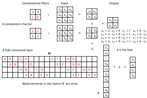
Refer to caption
Figure 9: The equivalence between a convolution channel and a matrix multiplication.

Assuming a CNN={𝒙;π’‡πŸ;…;𝒇𝑰;𝒇𝒀}CNN𝒙subscript𝒇1bold-…subscript𝒇𝑰subscript𝒇𝒀\text{CNN}=\{\boldsymbol{x;f_{1};...;f_{I};f_{Y}}\} has two adjacent convolutional layers π’‡π’Šsubscriptπ’‡π’Š\boldsymbol{f_{i}} and π’‡π’Š+𝟏subscriptπ’‡π’Š1\boldsymbol{f_{i+1}}. The first convolutional layer has N𝑁N channels, i.e. π’‡π’Š={π’‡π’Šπ’}n=1Nsubscriptπ’‡π’Šsuperscriptsubscriptsubscriptsuperscriptπ’‡π’π’Šπ‘›1𝑁\boldsymbol{f_{i}}=\{\boldsymbol{f^{n}_{i}}\}_{n=1}^{N}, and the second convolutional layer has K𝐾K channels, i.e. π’‡π’Š+𝟏={π’‡π’Š+πŸπ’Œ}k=1Ksubscriptπ’‡π’Š1superscriptsubscriptsubscriptsuperscriptπ’‡π’Œπ’Š1π‘˜1𝐾\boldsymbol{f_{i+1}}=\{\boldsymbol{f^{k}_{i+1}}\}_{k=1}^{K}. Therefore, the dimension of the convolutional filters π‘Ίπ’Š+𝟏subscriptπ‘Ίπ’Š1\boldsymbol{S_{i+1}} in π’‡π’Š+𝟏subscriptπ’‡π’Š1\boldsymbol{f_{i+1}} are WΓ—HΓ—NΓ—Kπ‘Šπ»π‘πΎW\times H\times N\times K, i.e., the dimension of a single filter connecting the π’‡π’Šπ’subscriptsuperscriptπ’‡π’π’Š\boldsymbol{f^{n}_{i}} channel and the π’‡π’Š+πŸπ’Œsubscriptsuperscriptπ’‡π’Œπ’Š1\boldsymbol{f^{k}_{i+1}} channel are D​(π‘Ίπ’Š+𝟏(π’Œ,𝒏))=WΓ—H𝐷subscriptsuperscriptπ‘Ίπ’Œπ’π’Š1π‘Šπ»D(\boldsymbol{S^{(k,n)}_{i+1}})=W\times H. As a result, the π’‡π’Š+πŸπ’Œsubscriptsuperscriptπ’‡π’Œπ’Š1\boldsymbol{f^{k}_{i+1}} channel can be formulated as

π’‡π’Š+πŸπ’Œ=Οƒi+1​(βˆ‘n=1Nπ‘Ίπ’Š+𝟏(π’Œ,𝒏)βˆ˜π’‡π’Šπ’+bi+1kβ‹…πŸ)subscriptsuperscriptπ’‡π’Œπ’Š1subscriptπœŽπ‘–1superscriptsubscript𝑛1𝑁subscriptsuperscriptπ‘Ίπ’Œπ’π’Š1subscriptsuperscriptπ’‡π’π’Šβ‹…subscriptsuperscriptπ‘π‘˜π‘–11\boldsymbol{f^{k}_{i+1}}=\sigma_{i+1}(\sum_{n=1}^{N}\boldsymbol{S^{(k,n)}_{i+1}}\circ\boldsymbol{f^{n}_{i}}+b^{k}_{i+1}\cdot\boldsymbol{1}) (45)

where Οƒi+1subscriptπœŽπ‘–1\sigma_{i+1} is the activation function and bi+1subscript𝑏𝑖1b_{i+1} is the bias for the (i+1)𝑖1(i+1)th channel.

We can regard the convolutional channel π’‡π’Š+πŸπ’Œsubscriptsuperscriptπ’‡π’Œπ’Š1\boldsymbol{f^{k}_{i+1}} as a matrix multiplication. The weights of the matrix depend on the convolutional filter and the spatial location of the convolutional output, and the output of the matrix multiplication is the vectorized output of the convolutional channel.

Without considering the activation function, the equivalence between a convolutional channel and a matrix multiplication can be explained in Figure 9, in which the first convolutional layer has two channels, i.e., π’‡π’Š={𝒙;𝒙^}subscriptπ’‡π’Šπ’™bold-^𝒙\boldsymbol{f_{i}}=\{\boldsymbol{x};\boldsymbol{\hat{x}}\}, where 𝒙={x1,β‹―,x9}𝒙subscriptπ‘₯1β‹―subscriptπ‘₯9\boldsymbol{x}=\{x_{1},\cdots,x_{9}\} and 𝒙^={x^1,β‹―,x^9}bold-^𝒙subscript^π‘₯1β‹―subscript^π‘₯9\boldsymbol{\hat{x}}=\{\hat{x}_{1},\cdots,\hat{x}_{9}\}, and the kπ‘˜kth channel of the second convolutional layer is π’‡π’Š+πŸπ’Œ={z1,z2,z3,z4}subscriptsuperscriptπ’‡π’Œπ’Š1subscript𝑧1subscript𝑧2subscript𝑧3subscript𝑧4\boldsymbol{f^{k}_{i+1}}=\{z_{1},z_{2},z_{3},z_{4}\}. In addition, the dimension of the convolutional filter π‘Ίπ’Š+𝟏subscriptπ‘Ίπ’Š1\boldsymbol{S_{i+1}} is 2Γ—2Γ—2Γ—122212\times 2\times 2\times 1, where π‘Ίπ’Š+𝟏(π’Œ,𝟏)=[A,B;C,D]subscriptsuperscriptπ‘Ίπ’Œ1π’Š1𝐴𝐡𝐢𝐷\boldsymbol{S^{(k,1)}_{i+1}}=[A,B;C,D] and π‘Ίπ’Š+𝟏(π’Œ,𝟐)=[E,F;G,H]subscriptsuperscriptπ‘Ίπ’Œ2π’Š1𝐸𝐹𝐺𝐻\boldsymbol{S^{(k,2)}_{i+1}}=[E,F;G,H]. Figure 9 shows that the output of π’‡π’Š+πŸπ’Œsubscriptsuperscriptπ’‡π’Œπ’Š1\boldsymbol{f^{k}_{i+1}} can be expressed as a matrix multiplication.

If we consider the activation function and make a precise statement, π’‡π’Š+πŸπ’Œsubscriptsuperscriptπ’‡π’Œπ’Š1\boldsymbol{f^{k}_{i+1}} can be formulated as

π’‡π’Š+πŸπ’Œ=Οƒi+1​(π‘Ύπ’Š+πŸπ’Œβ‹…π’‡π’Š+bi+1kβ‹…πŸ)subscriptsuperscriptπ’‡π’Œπ’Š1subscriptπœŽπ‘–1β‹…subscriptsuperscriptπ‘Ύπ’Œπ’Š1subscriptπ’‡π’Šβ‹…subscriptsuperscriptπ‘π‘˜π‘–11\boldsymbol{f^{k}_{i+1}}=\sigma_{i+1}(\boldsymbol{W^{k}_{i+1}}\cdot\boldsymbol{f_{i}}+b^{k}_{i+1}\cdot\boldsymbol{1}) (46)

where π‘Ύπ’Š+πŸπ’Œsubscriptsuperscriptπ‘Ύπ’Œπ’Š1\boldsymbol{W^{k}_{i+1}} is the matrix corresponding to all the convolutional filters in the kπ‘˜kth channel.