Negativity Spectrum in the Random Singlet Phase

Abstract

Entanglement features of the ground state of disordered quantum matter are often captured by an infinite randomness fixed point that, for a variety of models, is the random singlet phase. Although a copious number of studies covers bipartite entanglement in pure states, at present, less is known for mixed states and tripartite settings. Our goal is to gain insights in this direction by studying the negativity spectrum in the random singlet phase. Through the strong disorder renormalization group technique, we derive analytic formulas for the universal scaling of the disorder averaged moments of the partially transposed reduced density matrix. Our analytic predictions are checked against a numerical implementation of the strong disorder renormalization group and against exact computations for the XX spin chain (a model in which free fermion techniques apply). Importantly, our results show that the negativity and logarithmic negativity are not trivially related after the average over the disorder.

I Introduction

Entanglement is fundamental in understanding quantum phases of matter Amico2007 ; Calabrese2009R ; Laflorencie2015 . Mathematically defined as a measure of non-separability on quantum states, its intrinsic non-local nature renders this quantity theoretically and experimentally challenging to measure Islam2015 . Let us first consider a bipartition of a system into two spatial regions ${A\cup B}$, with Hilbert space ${\mathcal{H}=\mathcal{H}_{A}\otimes\mathcal{H}_{B}}$, and a pure state ${|\Psi\rangle\in\mathcal{H}}$ with reduced density matrix ${\rho_{A}=\text{tr}_{B}|\Psi\rangle\langle\Psi|}$. The content of bipartite entanglement can be read from the Rényi entanglement entropies

$$S_{\alpha}(\rho_{A})=\frac{1}{1-\alpha}\log\text{tr}\left(\rho_{A}^{\alpha}\right),$$ (1)

and from their von Neumann limit

$$S(\rho_{A})=\lim_{\alpha\to 1}S_{\alpha}(\rho_{A})=-\text{tr}(\rho_{A}\log\rho_{A}).$$ (2)

The knowledge of $S_{\alpha}$ for positive values of $\alpha$ fixes the entire spectrum of $\rho_{A}$. The latter, usually referred to as entanglement spectrum, has been proven of fundamental value in a variety of frameworks, including topological properties of quantum matter Li2008 ; Regnault2009 ; Fidkowski2010 ; Lauchli2010 ; Yao2010 ; Pollmann2010B ; Dubail2011 ; Qi2012 ; Poilblanc2012 ; Cincio2013 ; Lundgren2016 , symmetry-broken phases Metlitski2011 ; Alba2013 ; Tubman2014 ; Kolley2013 ; Frerot2016 and many-body localization Yang2015 ; Geraedts2016 ; Serbyn2016 . For one-dimensional critical systems with an underlying conformal invariance, the distribution of eigenvalues of ${\rho_{A}}$ obeys a universal scaling law, depending only on the central charge Lefevre2008 ; Lauchli2013 ; Pollmann2010 ; Nakagawa2017 ; gs-18 ; Alba2018A . This distribution is of high importance to understand the effectiveness of some tensor network algorithms Tagliacozzo2008 ; Pollmann2009 ; Pirvu2012 .

The situation is more complicated when considering a bipartition of a system in a mixed state. Here the Rényi entropies (1) do not distinguish between classical and quantum correlations, and thus, they fail to characterize entanglement. The same issue arises when considering the mutual entanglement between subregions of a multipartite pure state. For concreteness, let us consider a tripartition $A_{1}\cup A_{2}\cup B$ of a pure state ${|\Psi\rangle\in\mathcal{H}=\mathcal{H}_{A_{1}}\otimes\mathcal{H}_{A_{2}}\otimes\mathcal{H}_{B}}$. Tracing out $B$, we obtain the reduced density matrix $\rho_{A}$ describing the subsystem ${A=A_{1}\cup A_{2}}$. The quantum correlations between $A_{1}$ and $A_{2}$ are encoded in the partially transposed reduced density matrix Peres1996 ; Horodecki1996 ; Simon2000 ; Werner2001 ; Giedke2001 ; Zyczkowski1998 ; Zyczkowski1999 $\rho_{A}^{T_{2}}$ and in its negative eigenvalues. The definition of $\rho_{A}^{T_{2}}$ is ${\langle uv|\rho_{A}^{T_{2}}|u^{\prime}v^{\prime}\rangle\equiv\langle uv^{\prime}|\rho_{A}|u^{\prime}v\rangle}$, with $\{u\}$ and $\{v\}$ being local bases of respectively ${\mathcal{H}_{A_{1}}}$ and ${\mathcal{H}_{A_{2}}}$. From $\rho_{A}^{T_{2}}$ one can extract measures of mutual entanglement such as the entanglement negativity ${\cal N}$ and the logarithmic negativity ${\cal E}$ Eisert1999 ; Lee2000 ; Vidal2002 ; Plenio2005

$$\mathcal{N}=\frac{\big{|}\big{|}\rho_{A}^{T_{2}}\big{|}\big{|}-1}{2},\quad\mathcal{E}=\log\big{|}\big{|}\rho_{A}^{T_{2}}\big{|}\big{|},$$ (3)

where ${\big{|}\big{|}\rho\big{|}\big{|}=\text{tr}\sqrt{\rho\rho^{\dagger}}}$ is the trace norm. For any given state, clearly ${\cal E}=\log(2{\cal N}+1)$. The (logarithmic) negativity has been studied in several contexts, ranging from harmonic chains and lattices Audenaert2002 ; Ferraro2008 ; Cavalcanti2008 ; Anders2008 ; Anders2008B ; Marcovitch2009 ; Sherman2016 ; Nobili2016 ; ez-16c ; mm-18 to quantum spin models Wichterich2009 ; Bayat2010 ; Bayat2010B ; Bayat2012 ; Wichterich2010 ; Santos2011 ; Grover2018 ; Javanmart2018 ; gbpb-19 ; cgs-19 ; sdhs-16 ; ksr-19 , from conformal and integrable field theories Calabrese2012B ; Calabrese2013B ; Calabrese2013C ; Alba2013C ; Coser2014 ; Calabrese2015B ; Nobili2015 ; Kulaxizi2014 ; Fournier2016 ; Bianchini2016 to non-equilibrium situations Coser2014 ; Eisler2014B ; Alba2018 ; Hoogeveen2015 ; Wen2015 ; Gullans2019 ; knr-19 and intrinsic and symmetry-protected topological orders Wen2016A ; Wen2016B ; Castelnovo2013 ; Lee2013 ; Hart2018 ; Pollmann2012C ; Shiozaki2017 ; Shapourian2017 ; Shiozaki2017 ; Shiozaki2018 . For fermionic models, it has been shown that the partial time-reversal transpose is a more appropriate object to characterise the entanglement in mixed states ez-15 ; Shapourian2017 ; Shiozaki2018 ; cw-16 ; hw-16 ; eez-16 ; ssr-17 ; sr-19 ; sr-19b ; ctc-16 . Finally, also experimental proposals for the measurement of negativity have recently appeared Gray2018 ; Cornfeld2018 .

It is not a surprise that the spectral density of ${\rho_{A}^{T_{2}}}$ contains more information about the entanglement between $A_{1}$ and $A_{2}$ than the negativities in Eq. (3). Such spectral density is usually referred to as negativity spectrum Ruggiero2016 and is fully characterized through the moments

$$M_{\alpha}^{T_{2}}=\text{tr}\left(\rho_{A}^{T_{2}}\right)^{\alpha}.$$ (4)

In the following we will refer to $M_{\alpha}^{T_{2}}$ as negativity moments. Notice that the trace norm in Eq. (3) may be obtained as the replica limitCalabrese2012B ; Calabrese2013B ${\big{|}\big{|}\rho_{A}^{T_{2}}\big{|}\big{|}=\lim_{\alpha\to 1/2}M_{2\alpha}^{T_{2}}}$.

The negativity spectrum so far has been investigated only for clean systems Ruggiero2016 ; Mbeng2017 ; Hassan2019A . On the other hand, when considering quenched disorder, static and dynamic properties of a system drastically change compared to the clean case. In fact, randomness usually plays a relevant role in the renormalization group sense. Remarkable examples are Anderson and many-body localization Anderson1958 ; Abrahams2010 ; Nandkishore15 ; Abanin2019 . Other well studied systems include a class of quantum spin chains where disorder induces a novel quantum critical phase Ma1979 ; Ma1980 ; Fisher92 ; Fisher92B ; Igloi05 ; Monthus2018 . This phase is characterized by the formation of spin singlets spreading over arbitrarily large distances, and for this reason, it is dubbed random singlet phase (RSP). Its features can be analytically accessed by the strong disorder renormalization group (SDRG) technique Igloi05 ; Monthus2018 . Concerning entanglement, it was found that the disorder-averaged entanglement entropy of the RSP follows a universal scaling law Refael2004 ; Laflorencie2005 ; Dechiara2006 ; Refael2009 . Similar results have been derived in other disordered fixed points and singlet phases Raul2006 ; Refael2007 ; Hoyos2007 ; Lin2007 ; Bonesteel2007 ; Binosi2007 ; Igloi2008 ; Fidkowski2008 ; Yu2008 ; Hoyos2011 ; Kovaks2009 ; Kovaks2012 ; Getelina2016 ; Laguna2016 ; Burrell2007 ; Igloi2012 ; Bardarson2012 ; asr-18 ; pcp-19 . Furthermore, the disorder-averaged entanglement spectrum Pouranyari2013 ; tmd-18 and its moments Fagotti2011 have been studied, as well as the low-lying excitations Ramirez2014 .

In the same fashion, the disorder-averaged logarithmic negativity displays a universal scaling law Ruggiero2016B , but the negativity spectrum in disordered systems has not been studied yet. This work provides a first analysis on the subject, focusing on the random singlet phase. In the spirit of Ref. Fagotti2011, we use renewal equations to find analytic formulas for the negativity moments. In particular, we work out analytic result for the the case of adjacent intervals which we test against a numerical implementation of the SDRG and against ab-initio simulations for the random XX spin-chain. Among the other results, we find that the logarithm and the average disorder do not commute, in the sense that ${\overline{\log M^{T_{2}}_{2\alpha}}\neq{\log\overline{M^{T_{2}}_{2\alpha}}}}$ even in the limit ${\alpha\to 1/2}$. A maybe surprising consequence is that the negativity and its logarithmic analogue are not trivially related after disorder average in the RSP. This is in contrast with the case of the entanglement entropy, where the logarithm and the disorder average commute in the replica limit ${\alpha\to 1}$Fagotti2011 .

The remaining of the paper is organized as follows. In Sec. II we review the strong disorder renormalization group and the random singlet phase for the systems of interest. In Sec. III, we explain how the negativity spectrum can be characterized by the negativity moments. We then introduce the renewal equation for the negativity generating function and work out the negativity moments for adjacent intervals. The analytic solutions are benchmarked numerically in Sec. IV. In the last section we discuss the obtained results and possible outlooks. In an appendix we report the results for the fermionic negativity moments of the same disordered model.

II Random singlet phase

The random singlet phase is the simplest infinite-randomness fixed point Igloi05 ; Monthus2018 ; Refael2009 . It describes, for example, the low-energy properties of the spin-1/2 disordered Heisenberg and XX chains, which are particular instances (respectively ${\Delta=1}$ and ${\Delta=0}$) of the random XXZ chain, with Hamiltonian

$$H=\sum_{i=1}^{L-1}J_{i}(\sigma_{i}^{x}\sigma_{i+1}^{x}+\sigma_{i}^{y}\sigma_{i+1}^{y}+\Delta\sigma_{i}^{z}\sigma_{i+1}^{z}).$$ (5)

Here ${\sigma_{i}^{\alpha}}$ (${\alpha=x,y,z}$) denotes the Pauli matrices at site $i$, and the $\{J_{i}\}$ are positive uncorrelated quenched random couplings drawn by a probability distribution $P(J)$. It has been shown that the low-energy/long-distance properties are disorder independent, i.e., they are the same for essentially any choice of $P(J)$ Fisher92 . In the numerical section of this paper, we exploit this freedom by restricting to the uniform distribution ${P(J)=1}$, with ${J\in[0,1]}$.

The random singlet phase emerges from the SDRG applied to Eq. (5). In this section we briefly review and discuss some useful properties.

II.1 Universality of the phase

For disordered spin systems, the usual space-block decimation Cardybook fails due to the inhomogeneity of the hamiltonian (5) within a single disorder realization. The rationale is instead to decimate through an energetic principle, where, at each renormalization step, the sites connected by the strongest coupling are projected onto their local ground state, i.e., the singlet state. These are effectively decoupled by the rest of the system, while the edge sites are connected by a renormalized coupling.

For concreteness, let us focus on the random Heisenberg chain, although a similar procedure holds also for the XX chain. We denote the strongest bond by ${\Omega=J_{j}=\max_{i}J_{i}}$ (for some $j$) and rewrite the Hamiltonian as ${H=H_{\Omega}+H_{\textup{edge}}+H_{\textup{rest}}}$, where

$$H_{\Omega}=\Omega\vec{\sigma}_{j}\cdot\vec{\sigma}_{j+1},$$ (6)

$$H_{\textup{edge}}=J_{\textup{L}}\vec{\sigma}_{j-1}\cdot\vec{\sigma}_{j}+J_{\textup{R}}\vec{\sigma}_{j+1}\cdot\vec{\sigma}_{j+2},$$ (7)

$$H_{\textup{rest}}=\sum_{i\neq j-1,j,j+1}J_{i}\vec{\sigma}_{i}\cdot\vec{\sigma}_{i+1}.$$ (8)

The first line gives the Hamiltonian of the strongest bond connecting the sites ${(j,j+1)}$. The Hamiltonian ${H_{\textup{edge}}}$ represents the interaction of these sites with the neighboring spins, while the last equation is the Hamiltonian of all the other degrees of freedom. For ${\Omega}$ positive, the ground state of $H_{\Omega}$ is the singlet state

$$|s_{j}\rangle\equiv\frac{|\uparrow_{j}\downarrow_{j+1}\rangle-|\downarrow_{j}\uparrow_{j+1}\rangle}{\sqrt{2}}.$$ (9)

These two sites forming a singlet can be now decoupled, while the edge spins ${(j-1,j+2)}$ interacts via an effective Hamiltonian $H_{\textup{eff}}$, obtained through second order perturbation theory in $1/\Omega$. Apart from an unimportant additive constant, this reads

$$H_{\textup{eff}}=\tilde{J}_{j-1}\vec{S}_{j-1}\cdot\vec{S}_{j+2},\qquad\tilde{J}_{j-1}=\frac{J_{\textup{L}}J_{\textup{R}}}{2\Omega}.$$ (10)

After this renormalization step, the Hamiltonian ${H^{\prime}=H_{\textup{eff}}+H_{\textup{rest}}}$ is of the same form as the initial $H$, and the procedure can be iterated. The single step is called Ma-Dasgupta rule Ma1979 ; Ma1980 and can be summarized as

$$\left(\dots,J_{\textup{L}},\Omega,J_{\textup{R}},\dots\right)_{L}\to\left(\dots,\frac{J_{\textup{L}}J_{\textup{R}}}{2\Omega},\dots\right)_{L-2}.$$ (11)

In the last equation, we specified that the chain length reduced from $L$ to $L-2$ in one renormalization step. We stress that the SDRG results are valid in the ${L\to\infty}$ limit, and finite size corrections are present when numerically implementing Eq. (11) (see Sec. IV.2).

Successive applications of the Ma-Dasgupta rule lead asymptotically to a product state of singlets at arbitrarily large distances, the so-called random singlet phase (RSP), depicted in Fig. 1. Here, singlets between more distant sites are generated at later SDRG steps.

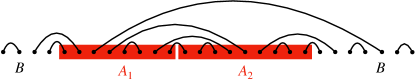
Figure 1: Cartoon of the random singlet phase in a tripartite setting ${A_{1}\cup A_{2}\cup B}$. The special case of two adjacent intervals (in red) embedded in a larger system is depicted.

In order to understand how universality emerges in the RSP phase, it is convenient to introduce the variables

$$\beta^{m}_{i}=\log\frac{\Omega^{(m)}}{J_{i}^{(m)}},\quad{\Gamma^{(m)}=-\log\Omega^{(m)}}.$$ (12)

Here ${\Omega^{(m)}}$ and ${J_{i}^{(m)}}$ are respectively the strongest bond and the couplings at site $i$ at renormalization step $m$. Intuitively, ${\Gamma}$ set the energy scale of the strongest coupling at a successive step, while ${\beta}$ is a measure of the broadness of the coupling distribution around it.

The Ma-Dasgupta rule (11) rewritten in terms of the $\beta$ variables is ${\tilde{\beta}=\beta_{\textup{L}}+\beta_{\textup{R}}-\log{2}}$. It induces a flow for the probability distribution of the couplings ${P(\beta,\Gamma)}$

$$\frac{d}{d\Gamma} P(\beta,\Gamma)=\frac{\partial}{\partial\beta}P(\beta,\Gamma)+P(0,\Gamma)\int_{0}^{\infty}d\beta_{2}\int_{0}^{\infty}d\beta_{1}$$

$$\times\delta(\beta_{1}+\beta_{2}-\log{2}-\beta)P(\beta_{1},\Gamma)P(\beta_{2},\Gamma).$$ (13)

Iterating the renormalization procedure, $\beta$ grows indefinitely and it is safe to drop out the factor $\log 2$ in the above equation. Within this assumption, Eq. (II.1) can be solved analytically Fisher92 , leading to

$$P_{\star}(\beta,\Gamma)=\frac{e^{-\beta/\Gamma}}{\Gamma}.$$ (14)

This function is a universal attractor, irrespective of the distribution of the couplings Fisher92 ; Fisher92B ; Refael2009 . Moreover, variables distributed according to Eq. (14) are closely packed around ${J_{\star}\simeq 0^{+}}$, and this a posteriori justifies the perturbative treatment.

We close by recalling that similar results hold for the XX chain, where the Ma-Dasgupta rule reads Igloi05

$$\left(\dots,J_{\textup{L}},\Omega,J_{\textup{R}},\dots\right)_{L}\to\left(\dots,\frac{J_{\textup{L}}J_{\textup{R}}}{\Omega},\dots\right)_{L-2}.$$ (15)

It is evident that the random XX and Heisenberg chains belong to the same universality class since they share the same fixed point distribution ${P_{\star}(\beta,\Gamma)}$.

II.2 Structure of the reduced density matrix and its partial transpose

The RSP emerges naturally as an infinite disorder critical point, and it is characterized by singlets spreading among arbitrary far regions of the system. Below we introduce the elementary building blocks of the associated density matrix and its partially transpose. They are (i) the density matrix of a singlet, $\rho_{\textup{2s}}$, (ii) its reduced density matrix for one of the spins, ${\rho_{\textup{s}}}$, (iii) the partial transpose of $\rho_{\textup{2s}}$ with respect to one of the sites, ${\rho_{\textup{2s}}^{T_{2}}}$. In the basis ${\left|\uparrow\uparrow\right\rangle}$, ${\left|\uparrow\downarrow\right\rangle}$, ${\left|\downarrow\uparrow\right\rangle}$, and ${\left|\downarrow\downarrow\right\rangle}$, the above objects read

$$\rho_{\textup{2s}}= \frac{1}{2}\begin{pmatrix}0&0&0&0\\ 0&1&-1&0\\ 0&-1&1&0\\ 0&0&0&0\end{pmatrix},\quad\rho_{\textup{s}}=\frac{1}{2}\begin{pmatrix}1&0\\ 0&1\end{pmatrix},$$ (16)

$$\qquad\rho^{T_{2}}_{\textup{2s}}=\frac{1}{2}\begin{pmatrix}0&0&0&-1\\ 0&1&0&0\\ 0&0&1&0\\ -1&0&0&0\end{pmatrix}.$$ (17)

For concreteness, we consider the partition of the system ${B\cup A_{1}\cup A_{2}}$ (pictorially represented in Fig. 1), with ${A=A_{1}\cup A_{2}}$. We denote with ${n_{X:Y}}$ the number of singlets shared between $X$ and $Y$. This is symmetric ${n_{X:Y}=n_{Y:X}}$ and additive ${n_{X:Y\cup Z}=n_{X:Y}+n_{X:Z}}$. The density matrix of the RSP takes the form

$$\rho_{\textup{RSP}}=\bigotimes_{m=1}^{n_{A:A}}\rho_{\textup{2s}}\bigotimes_{n=1}^{n_{A:B}}\rho_{\textup{2s}}\bigotimes_{l=1}^{n_{B:B}}\rho_{\textup{2s}}.$$ (18)

Tracing out $B$ we obtain

$$\rho_{A}=\bigotimes_{m=1}^{n_{A:A}}\rho_{\textup{2s}}\bigotimes_{n=1}^{n_{A:B}}\rho_{\textup{s}},$$ (19)

whose partial transpose with respect to $A_{2}$ gives

$$\rho_{A}^{T_{2}}=\bigotimes_{q=1}^{n_{A_{1}:A_{1}}}\rho_{\textup{2s}}\bigotimes_{r=1}^{n_{A_{2}:A_{2}}}\rho_{\textup{2s}}\bigotimes_{p=1}^{n_{A_{1}:A_{2}}}\rho^{T_{2}}_{\textup{2s}}\bigotimes_{n=1}^{n_{A:B}}\rho_{\textup{s}}.$$ (20)

Here we have used the fact that ${\rho_{\textup{s}}^{T_{2}}=\rho_{\textup{s}}}$ for a single site, and that ${\rho_{\textup{2s}}^{T_{2}}=\rho_{\textup{2s}}}$ when both the ends of a bond are in the same subsystem $A_{i}$ $(i=1,2)$. The spectrum of Eq. (20) is denoted as negativity spectrum and is the main object of study in this paper.

II.3 Scaling of the in-out bond

The density matrix of a single random configuration and all the quantities that can be derived from it are fully characterized by the number of in-out bonds $n_{X:Y}$. Consequently, the scaling of these quantities is crucial in the study of the spectrum of the reduced density matrix of the RSP and of its partial transpose. The knowledge of all the $n_{X:Y}$ can be extracted through the solution of a simple set of linear equations, relying on the additivity property of $n_{X:Y}$. Hereafter we denote by $\ell_{X}$ the length of an interval $X$, and ${{X}_{c}}$ its complement. Consider a $2k$-multipartite system ${\bigcup_{X\in\mathcal{G}_{0}}}X$ with ${\mathcal{G}_{0}=\{A_{1},B_{1},\dots,A_{k},B_{k}\}}$. We define ${\mathcal{G}}$ as the set of all possible compact subintervals of the chain. For each ${X\in\mathcal{G}}$ one can decompose the number of singlets $n_{X:X_{c}}$ as

$$n_{X:X_{c}}=\sum_{Y,Z\in\mathcal{G}}n_{X\cap Y:X_{c}\cap Z}.$$ (21)

After taking the disorder average, we have a set of linear equations, whose solution gives $\overline{n}_{X:W}$ for any ${X,W\in\mathcal{G}_{0}}$

$$\overline{n}_{X:X_{c}}=\sum_{Y,Z\in\mathcal{G}}\overline{n}_{X\cap Y:X_{c}\cap Z}.$$ (22)

The left hand side has been previously computed within the RSP Refael2004

$${\overline{n}_{X:X_{c}}=\frac{b_{X:X_{c}}}{6}\log\ell_{X}+k},$$ (23)

where $b_{X:X_{c}}$ is the number of edges shared by $X$ and $X_{c}$, and $k$ is a non-universal constant of order ${\mathcal{O}(1)}$ in the subsystem size $\ell_{X}$. For the leading logarithmic term, we then have

$$\frac{b_{X:X_{c}}}{6}\log\ell_{X}=\sum_{Y,Z\in\mathcal{G}}\overline{n}_{X\cap Y:X_{c}\cap Z}.$$ (24)

This set of equations can be straightforwardly solved for the variables $\overline{n}$, and a unique solution can be extracted for any partition of the system. See Ref. Ruggiero2016B, for several explicit examples.

III Negativity spectrum

III.1 Logarithmic negativity and negativity moments

The central object of this paper is the spectral density of the operator ${\rho_{A}^{T_{2}}}$ in Eq. (20)

$$\mathbb{P}(\lambda)=\sum_{i}\delta(\lambda-\lambda_{i}),$$ (25)

where the sum is over the eigenvalues of ${\rho_{A}^{T_{2}}}$. From the knowledge of ${\mathbb{P}(\lambda)}$, we can infer the negativity moments (4)

$$\text{tr}(\rho_{A}^{T_{2}})^{\alpha}=\sum_{i}\lambda_{i}^{\alpha}=\int d\lambda\,\mathbb{P}(\lambda)\lambda^{\alpha}.$$ (26)

The converse is also true, in that the knowledge of all the negativity moments gives access to the function ${\lambda\mathbb{P}(\lambda)}$ through an inverse Stieltjes transform Ruggiero2016 ; Hassan2019A . For this reason, with a slight but standard abuse of language, we will refer also to the whole set of moments as the negativity spectrum.

Most of the derivations presented in this section are valid for a very general tripartition $A_{1}\cup A_{2}\cup B$ of an infinite chain (with some caveat which will be clearer in the course of the calculation). At the very end of the section, for concreteness, we will specialize to the usual partition depicted in Fig. 1 with two adjacent blocks.

Within a single disorder realization, the negativity moments depends only on ${n_{A:B}}$ and ${n_{A_{1}:A_{2}}}$. The partial transpose ${\rho_{A}^{T_{2}}}$ in Eq. (20) is straightforwardly diagonalized and the eigenvalues are

$$\lambda_{\pm}=\pm 2^{-n_{A:B}-n_{A_{1}:A_{2}}},$$ (27)

with degeneracies

$$d_{-} =2^{n_{A:B}+n_{A_{1}:A_{2}}-1}(2^{n_{A_{1}:A_{2}}}-1),$$ (28)

$$d_{+} =2^{n_{A:B}+2n_{A_{1}:A_{2}}}-d_{-}.$$ (29)

Consequently, the negativity moments for this given disorder realization are

$$M^{T_{2}}_{\alpha}=2^{(n_{A:B}+n_{A_{1}:A_{2}})(1-\alpha)}\begin{cases}2^{n_{A_{1}:A_{2}}}&\alpha\,\text{even}\\ 1&\alpha\,\text{odd}.\end{cases}$$ (30)

Notice that the moments $M^{T_{2}}_{\alpha}$ depends on both $n_{A:B}$ and $n_{A_{1}:A_{2}}$. Hence, as well known, they are not direct measures of the mutual entanglement between $A_{1}$ and $A_{2}$. However, the dependence on $n_{A:B}$ cancels in the limit $2\alpha\to 1$, as a consequence of the fact that the negativity is a good entanglement measure also in the RSPRuggiero2016B . Nevertheless, in the same spirit of the entanglement spectrum compared to the entanglement entropyLi2008 , the moments (30) encode more information about the mutual entanglement than the (logarithmic) negativity itself, as we shall see.

Till now we have been discussing what happens for a single disorder realization, but the physical relevant quantities are the averages over the quench disorder. From the knowledge of the moments, we can define two different averaged quantities, each one providing useful information about the entanglement. Indeed, since the average of the logarithm and the logarithm of the average are not at all equivalent, we can define

$$\hat{\mathcal{E}}_{\alpha} =\overline{\log M_{\alpha}^{T_{2}}},$$ (31)

$${\mathcal{E}}_{\alpha} =\log\overline{M_{\alpha}^{T_{2}}}.$$ (32)

These two quantities are expected to behave very differently, as it happens for the analogous averages for the entanglement spectrum Fagotti2011 (i.e. $\overline{\log{\rm tr}\rho_{A}^{\alpha}}$ and $\log\overline{{\rm tr}\rho_{A}^{\alpha}}$). Anyhow, we are going to show that $\hat{\mathcal{E}}_{\alpha}$ and ${\mathcal{E}}_{\alpha}$ are related through a linear transformation at the leading order in $\ell$.

III.2 Moments $\hat{\mathcal{E}}_{\alpha}$ and logarithmic negativity

We start by considering the average of the logarithm of the moments ${\hat{\mathcal{E}}_{\alpha}}$ ($\alpha>0$) in (31). This is the easiest quantity to calculate because it depends linearly on $\overline{n}_{A:B}$ and $\overline{n}_{A_{1}:A_{2}}$. Hence, straightforwardly from Eq. (30), we get

$$\hat{\mathcal{E}}_{\alpha}=\log 2\begin{cases}(1-\alpha)\overline{n}_{A:B}+(2-\alpha)\overline{n}_{A_{1}:A_{2}}&\alpha\,\text{even,}\\ (1-\alpha)(\overline{n}_{A:B}+\overline{n}_{A_{1}:A_{2}})&\alpha\,\text{odd}.\end{cases}$$ (33)

We observe that, because of the linear structure, $\hat{\mathcal{E}}_{\alpha}$ depends only on the averages $\bar{n}_{X:Y}$ and not on the full distribution of the singlets shared between the partitions. We recall that one of the main reasons why we are interested in $\hat{\mathcal{E}}_{\alpha}$ is that they are the replica quantities to access the average logarithmic negativity Ruggiero2016B

$$\mathcal{E}=\lim_{\alpha\to 1/2}\hat{\mathcal{E}}_{2\alpha}=\overline{n}_{A_{1}:A_{2}}\log 2.$$ (34)

We stress that (33) are valid for arbitrary tripartition of the chain and not only for adjacent intervals. Notice that since the moments $\hat{\mathcal{E}}_{\alpha}$ depend only on the averages $\bar{n}_{X:Y}$, they do not encode more information than the entanglement negativity and entropy.

III.3 Moments ${\mathcal{E}}_{\alpha}$ and renewal equation for the negativity spectrum

The logarithm of the average of the moments in Eq. (32) is the quantity more directly related to the true negativity spectrum (i.e. the distribution of eigenvalues of the partial transpose). Its calculation is, however, much more cumbersome compared to $\hat{\mathcal{E}}_{\alpha}$ because of the non-linear dependence on $n_{X:Y}$: it requires the knowledge of the entire distribution of singlets and not only of the average. We focus on the tripartition ${A=A_{1}\cup A_{2}}$ and ${B=A_{c}}$. Denoting as ${P(n_{A:B},n_{A_{1}:A_{2}})}$ the joint probability distribution of $n_{A:B}$ and $n_{A_{1}:A_{2}}$, we introduce the generating function for the probability distribution of in-out bonds Fagotti2011 ; Vasseur2015 .

$$g(t,s)\equiv\log\langle e^{tn_{A:B}+sn_{A_{1}:A_{2}}}\rangle=\\ =\log\sum_{n_{A:B},n_{A_{1}:A_{2}}}e^{n_{A:B}t+n_{A_{1}:A_{2}}s}P(n_{A:B},n_{A_{1}:A_{2}}).$$ (35)

The knowledge of $g(t,s)$ is equivalent to the that of the negativity spectrum, in the sense that it univocally determines the negativity moments.

The asymptotic behavior of generating function $g(t,s)$ (in a RG sense that will be clearer later on) may be accessed following the phenomenological approach introduced in Ref. Fagotti2011, for the entanglement spectrum. The starting observation is that, within SDRG, the singlets form at a constant rate with respect to the RG time $\mu$. This rate is responsible for the logarithmic scaling of ${\overline{n}_{X:X_{c}}}$ for a single interval $X$. The probability distribution of waiting times for a decimation to occur across a bond since the last decimation is Refael2004

$$f(\mu)=\frac{1}{\sqrt{5}}\left(e^{-\frac{3-\sqrt{5}}{2}\mu}-e^{-\frac{3+\sqrt{5}}{2}\mu}\right).$$ (36)

This expression is true only for asymptotically large $\mu$ because non-universal terms related to the initial distribution of disorder have been neglected in its derivation Refael2004 . For the following, it is useful to explicitly introduce $\tilde{f}(x)$ as the Laplace transform of $f(\mu)$

$$\tilde{f}(x)=\frac{1}{\sqrt{5}}\left(\frac{1}{x+\frac{3-\sqrt{5}}{2}}-\frac{1}{x+\frac{3+\sqrt{5}}{2}}\right).$$ (37)

At this point, in order to compute $g(t,s)$ one would need to know and quantify all the possible processes between two RG times. The renormalization flow generate several of these processes, but the most probable one is clearly the formation of isolated singlets Fagotti2011 . Thus, in a first approximation, expected to be correct in the limit of large $\mu$, we can write a renewal equation for the generating function (35), considering only formations of in-out isolated singlets

$$\langle e^{nt+sm}\rangle_{\mu}=\int_{\mu}^{\infty}d\xi f(\xi)+pe^{t}\int_{0}^{\mu}d\xi f(\xi)\langle e^{nt+sm}\rangle_{\mu-\xi}\\ +qe^{s}\int_{0}^{\mu}d\xi f(\xi)\langle e^{nt+sm}\rangle_{\mu-\xi}.$$ (38)

Here, for notational convenience, we express the disorder average at RG time $\mu$ with ${\langle\cdot\rangle_{\mu}}$ while $n$ and $m$ are just shorthands for $n_{A:B}$ and $n_{A_{1}:A_{2}}$ respectively. The constants $p$ and $q=1-p$ are, respectively, the asymptotic probability of increasing ${n}$ and ${m}$ by one unit. In a general setting $p$ and $q$ can depend on the RG time $\mu$ and can have activation times depending on the tripartition, here we are only interested in the limit of large $\mu$ and hence neglect these corrections that can be important when comparing with numerics. The fundamental assumption here is that $p$ and $q$ have a non-zero limit as ${\mu\to\infty}$. The renewal equation (38) represents an educated conjecture generalizing the one for $n_{A:B}$ in Ref. Fagotti2011, to two kinds of singlets ($n_{A:B}$ and $n_{A_{1}:A_{2}}$) with probability $p$ and $q$. The correctness of all our (reasonable) assumptions can be tested only a posteriori with numerical simulations.

The renewal equation (38) can be solved through Laplace transform. Indeed, after some simple algebra we get

$$g_{\mu}(t,s)=\log\left[\mathcal{L}^{-1}\left(\frac{1}{x}\frac{1-\tilde{f}(x)}{1-(pe^{t}+qe^{s})\tilde{f}(x)}\right)(\mu)\right].$$ (39)

The inverse transform $\mathcal{L}^{-1}$ can be computed analytically and gives, at large $\mu$

$$e^{g_{\mu}(t,s)}\stackrel{{\scriptstyle\mu\gg 1}}{{\simeq}}\left(\frac{1}{2}+\frac{3}{2\sqrt{5+4(pe^{t}+qe^{s})}}\right)\times\\ \qquad\qquad\exp{\displaystyle\left(\frac{\sqrt{5+4(pe^{t}+qe^{s})}-3}{2}\mu\right)}.$$ (40)

From the definition (35), we have

$$\overline{n}_{A_{1}:A_{2}}=\partial_{s}g(0,0) \stackrel{{\scriptstyle\mu\gg 1}}{{=}}\frac{q}{9}(3\mu-1),$$ (41)

$$\overline{n}_{A:B}=\partial_{t}g(0,0) \stackrel{{\scriptstyle\mu\gg 1}}{{=}}\frac{p}{9}(3\mu-1),$$ (42)

and in particular

$$\frac{\overline{n}_{A_{1}:A_{2}}}{\overline{n}_{A:B}}=\frac{q}{p}=\frac{q}{1-q}.$$ (43)

The last three equations must be used to extract $p$ and ${q=1-p}$ in a self-consistent way. Indeed, the average number of singlets between complementary sets is univocally fixed by the set of equations (24). Thus, for a chosen partitioning $\mathcal{G}_{0}$, one first solves (24), then uses the solutions to determine the probabilities $p$ and $q$ via Eq. (43), and finally plug them in Eq. (39) determining the asymptotics of $g(t,s)$ for large $\mu$. Notice that in Eqs. (41) and (42) we kept the $O(1)$ term in $\mu$ to show that Eq. (43) is valid also at the first subleading order.

At this point, Eq. (30) allows to write the desired averaged negativity moments as function of $g(t,s)$ as

$$\mathcal{E}_{\alpha}=g(t_{\alpha},s_{\alpha}),$$ (44)

with

$$t_{\alpha} \equiv (1-\alpha)\log 2,$$ (45)

$$s_{\alpha} \equiv \begin{cases}(2-\alpha)\log 2&\alpha\,\text{even},\\ (1-\alpha)\log 2&\alpha\,\text{odd}.\end{cases}$$ (46)

The leading term in $\mu$ (and hence in $\overline{n}$ or equivalently in $\ell$) comes from the exponential term in Eq. (40). We have two different results for $\alpha$ even and odd that we denote respectively as $\mathcal{E}^{e}_{\alpha}$ and $\mathcal{E}^{o}_{\alpha}$. By simple algebra we obtain

$$\mathcal{E}^{e}_{\alpha}=\frac{\sqrt{5+(1+q)2^{3-\alpha}}-3}{2}\mu+\dots,$$ (47)

and

$$\mathcal{E}^{o}_{\alpha}=\frac{\sqrt{5+2^{3-\alpha}}-3}{2}\mu+\dots,$$ (48)

where the dots stands for subleading non-universal terms in $\mu$. Notice that in Eqs. (47) and (48) all the dependence on the partition is encoded in the constant $q$ and in $\mu$. However, since $\mu$ is proportional to the logarithm of the length involved in the problem, the universal prefactor of this logarithm depends on the partition only through $q$. Hence, the odd moments have the same scaling factor for any tripartition of the chain with ${q\neq 0,1}$.

Eqs. (47) and (48) are the main analytic results of this manuscript and we recall that they are valid for any tripartition of the infinite chain as long as ${p,q\neq 0}$. They contain a lot of physical insights that we are going to discuss now. First of all, they depend on the entire distribution of shared singlets and not only on they averaged values, showing indeed that the negativity moments provide more information than the logarithmic negativity and the entanglement entropy. A trivial consistency check is that ${{\cal E}^{o}_{1}=0}$, as it should. An important consequence of Eq. (47) is that the replica limit ${{\cal E}^{e}_{1}={\lim_{\alpha\to 1}\mathcal{E}_{2\alpha}}}$ does not converge to the logarithmic negativity Eq. (34) (which is the limit of $\hat{\mathcal{E}}_{2\alpha}$) for any $q>0$. This means that the average negativity is not related trivially to the average logarithmic negativity as instead happens for a clean system, i.e. ${\overline{\cal E}\neq\log(2\overline{\cal N}-1)}$ as average over disorder. Not only, we also have that ${{{\cal E}^{e}_{1}>\hat{\cal E}^{e}_{1}}}$ for all $q>0$, as expected since the logarithm is a concave function. It is also true that ${{{\cal E}_{\alpha}>\hat{\cal E}_{\alpha}}}$ for any $\alpha$.

Since both ${\cal E}_{\alpha}$ and $\hat{\cal E}_{\alpha}$ are proportional to $\mu$, it is instructive also to write a relation between the two at fixed $\alpha$. Simply combining Eqs. (47) and (48) with (33), we obtain

$$\mathcal{E}_{\alpha}=A_{\alpha}\hat{\mathcal{E}}_{\alpha}+K^{(\alpha)},$$ (49)

were ${K^{(\alpha)}}$ are a non-universal constants and function $A_{\alpha}$ takes two different values for even and odd $\alpha$:

$$A_{\alpha}^{e} = 3\frac{\sqrt{5+(1+q)2^{3-\alpha}}-3}{2(1-\alpha+q)\log 2},$$ (50)

$$A_{\alpha}^{o} = 3\frac{\sqrt{5+2^{3-\alpha}}-3}{2(1-\alpha)\log 2}.$$ (51)

III.4 Application to adjacent intervals

In this subsection we specialize the results of the previous one to the case of adjacent intervals of length $\ell_{1}$ and $\ell_{2}$ as in Fig. 1. In this case the set of equations (24) admits the following solution at the leading order in the lengths Ruggiero2016B

$$\overline{n}_{A_{1}:A_{2}}=\frac{1}{6}\log\left(\frac{\ell_{A_{1}}\ell_{A_{2}}}{\ell_{A_{1}}+\ell_{A_{2}}}\right),$$ (52)

$$\overline{n}_{A:B}=\frac{1}{3}\log{(\ell_{A_{1}}+\ell_{A_{2}})}.$$ (53)

The ratio (43) seems a complicated function of $\ell_{1}$ and $\ell_{2}$. However, we are interested in the regime of ${\ell_{1}\propto\ell_{2}\gg 1}$ when ${\overline{n}_{A_{1}:A_{2}}/\overline{n}_{A:B}=1/2+\dots}$, where the dots stand for subleading logarithmic corrections to the scaling (which may be important in the analysis of the numerical data). Hence, in the regime ${\ell_{1,2}\gg 1}$, from Eq. (43) we get

$$q=\frac{1}{3},\quad{\rm and}\quad p=\frac{2}{3}.$$ (54)

Summarizing, plugging Eq. (54) in Eqs. (33), (47) and (48), the final results for $\hat{\mathcal{E}}_{\alpha}$ and ${\mathcal{E}}_{\alpha}$ for adjacent intervals are

$$\hat{\mathcal{E}}_{\alpha}^{e} = (4-3\alpha)\frac{\log 2}{6}\log{\ell}+\dots,$$ (55)

$$\hat{\mathcal{E}}_{\alpha}^{o} = (1-\alpha)\frac{\log 2}{2}\log{\ell}+\dots,$$ (56)

$${\mathcal{E}}_{\alpha}^{e} = 3\frac{\sqrt{5+2^{5-\alpha}/3}-3}{4}\log\ell+\dots,$$ (57)

$${\mathcal{E}}_{\alpha}^{o} = 3\frac{\sqrt{5+2^{3-\alpha}}-3}{4}\log\ell+\dots,$$ (58)

where we posed ${\ell=\ell_{1}=x\ell_{2}}$ (with $x$ finite) and the dots stand (again) for non-universal additive constants (with a partial and universal dependence on $x$).

The relation between $\hat{\mathcal{E}}_{\alpha}$ and ${\mathcal{E}}_{\alpha}$ is always given by Eq. (49) with $A^{o}_{\alpha}$ given by Eq. (51) and $A^{e}_{\alpha}$ equal to

$$A_{\alpha}^{e} =9\frac{\sqrt{5+2^{5-\alpha}/3}-3}{2(4-3\alpha)\log 2}.$$ (59)

The above results straightforwardly generalize to more involved tripartitions and can be used to access universal features of the negativity spectrum in the RSP. Let us recapitulate what one has to do in the most general case: (i) choose the partition, (ii) compute the average in-out singlets number solving the set of equations (24), (iii) find the values of $p$ and $q$ using Eq. (43), (iv) if $p,q\neq 0$, then the negativity moments are just given by Eqs. (47) and (48). The results will be valid only in the scaling regime of all length-scales of the same order and much larger than $1$.

IV Numerical tests for adjacent intervals

In this section we numerically test the predictions reported above and in particular we compare our numerical simulations with the analytic formulas (55-58) for the negativity moments of adjacent intervals. We focus on the XX chain for which we can exploit known free fermion techniques to easily access the integer moments ${M^{T_{2}}_{\alpha}}$ with ab-initio simulations Fagotti2010B ; Coser2014 ; Eisler2014B ; Coser2015 . This kind of computations does not rely on the random singlet phase structure and thus represents a robust non-trivial check of our findings. We also implement numerically the SDRG providing another numerical benchmark which allows to explore much larger system sizes and easily access also the two analytic continuations of the moments to non-integer values. All these simulations are extremely important in view of the several (reasonable) assumptions we made in writing down the renewal equation (38): only the very good agreement between the predictions from its solution and the numerics represents a definitive confirmation for the correctness of these assumptions, at least for asymptotically large RG time.

IV.1 Free fermions and negativity spectrum

We review the mapping between the XX chain and free fermions on the line. Within the free fermions formalism, we can express the reduced density matrix and its partial transpose in the spin variables as a sum of Gaussian operators with known Majorana correlation matrices. The negativity moments are computed through a product rule for Gaussian matricesbb-69 ; Fagotti2010B ; Coser2015 .

The Hamiltonian of the random XX chain is Eq. (5) at ${\Delta=0}$

$$H=\sum_{i=1}^{L-1}J_{i}(\sigma_{i}^{x}\sigma_{i+1}^{x}+\sigma_{i}^{y}\sigma_{i+1}^{y}).$$ (60)

Here we consider a chain of length $L$. The Jordan-Wigner transformation

$$c_{i}=\left(\prod_{m=1}^{i-1}\sigma^{z}_{m}\right)\frac{\sigma_{i}^{x}-i\sigma^{y}_{i}}{2},$$ (61)

maps the Hamiltonian (60) in the free-fermion one

$$H=\frac{1}{2}\sum_{i=1}^{L-1}J_{i}(c_{i}^{\dagger}c_{i+1}+c_{i+1}^{\dagger}c_{i})\equiv\sum_{i,j=1}^{L-1}c_{i}^{\dagger}h_{i,j}c_{j}.$$ (62)

The $c_{i}$ are fermion annihilation operator, satisfying the canonical anti-commutation relations ${\{c_{m},c_{n}^{\dagger}\}=\delta_{mn}}$. At the free fermion point the many-body eigenfunctions of $H$ can be expressed in terms of the single-particle ones $\{\phi_{q}(i)\}$; the same is true for the many-body spectrum. Indeed, the eigenstates of the Hamiltonian (62) are obtained by applying an arbitrary number of single-particle creation operators

$$\eta_{q}^{\dagger}=\sum_{i}\phi_{q}(i)c_{i}^{\dagger},$$ (63)

to the (fermonic) vacuum ${|0\rangle}$. The ground state of (60) corresponds to half-filling in fermionic language, that is the $N=L/2$ lowest energy levels are occupied

$$|\textup{GS}\rangle=\eta_{q_{N}}^{\dagger}\cdots\eta_{q_{1}}^{\dagger}|0\rangle.$$ (64)

The correlation matrix takes the form

$$C_{ij}\equiv\langle c_{i}^{\dagger}c_{j}\rangle=\sum_{q}\phi_{q}^{*}(i)\phi_{q}(j),$$ (65)

where the sum is over the occupied single-particle excitations in the ground state. The reduced correlation matrix to a given subsystem $A$ with $\ell$ sites, ${C_{A}}$, is a ${\ell\times\ell}$ matrix whose elements are defined by the restriction of Eq. (65) to ${i,j\in A}$. For later convenience we also introduce the Majorana fermions

$$a_{2m-1}=c_{m}^{\dagger}+c_{m},\quad a_{2m}=i(c_{m}^{\dagger}-c_{m}),$$ (66)

and the corresponding ${2\ell\times 2\ell}$ Majorana correlation matrix $\Gamma_{A}$ with matrix elements

$$(\Gamma_{A})_{nm}\equiv\langle a_{m}a_{n}\rangle-\delta_{mn}.$$ (67)

It is clear that there is a direct relation between the entries of $\Gamma_{A}$ and those of $C_{A}$.

Crucially, reduced density matrices associated with a single interval are Gaussian operators Peschel2009

$$\rho_{A}=\frac{1}{Z_{\Omega}}\exp\left(\frac{1}{4}\sum_{n,m}a_{n}\Omega_{nm}a_{m}\right),$$ (68)

($Z_{\Omega}$ being a normalization) and the matrix $\Omega$ may be written in terms of $\Gamma_{A}$ as

$$\Gamma_{A}\equiv\tanh\left(\frac{\Omega}{2}\right).$$ (69)

However, when the subsystem $A$ consists of more than one interval, the reduced density matrix is not gaussian ip-09 ; atc-09 , and so also its partial transpose ez-15 ; Coser2015 . Still, in both cases, the corresponding operator is the sum of gaussian terms. For instance, in the case of two disjoint intervals ${A=A_{1}\cup A_{2}}$, $\rho_{A}$ is the sum of two Gaussian operators $\rho_{\Gamma_{i}}$ associated by Eqs. (68) and (69) to distinct covariance matrices $\Gamma_{i}$.

With free fermion techniques is not straightforward to calculate the eigenvalues of the sum of Gaussian operators (see anyhow Ref. zrc-19, for a brute force approach). Instead, the traces of arbitrary integer powers of sums of (even non-commuting) gaussian operators can be calculated with, by now, standard methods bb-69 ; Fagotti2010B . These methods heave been exploited already many times also for the calculation of negativity in spin chains ez-15 ; Coser2015 ; Nobili2015 ; ctc-16 . Since the associated machinery is quite involved, here we just summarize the results and refer to the literature for further details ez-15 ; Coser2015 . Let us denote by $\rho_{\Gamma}$ the gaussian operator associated to the covariance matrix $\Gamma$. Given $\Gamma$ and $\Gamma^{\prime}$, we define the following product rule

$$\rho_{\Gamma}\rho_{\Gamma^{\prime}}={\rm Tr}\left[\rho_{\Gamma}\rho_{\Gamma^{\prime}}\right]\;\rho_{\Gamma\times\Gamma^{\prime}},$$ (70)

where Fagotti2010B

$$\Gamma\times\Gamma^{\prime}\equiv 1-(1-\Gamma^{\prime})\frac{1}{1+\Gamma\Gamma^{\prime}}(1-\Gamma),$$ (71)

relating the covariance matrices of two gaussian operators to the one associated to their product. The trace on the right hand side of (70) isbb-69 ; Fagotti2010B

$$\{\Gamma,\Gamma^{\prime}\}\equiv{\rm Tr}\left(\rho_{\Gamma}\rho_{\Gamma^{\prime}}\right)=\prod_{\mu\in\sigma(\Gamma\Gamma^{\prime})/2}\frac{1+\mu}{2},$$ (72)

with the product being over half of the spectrum ${\sigma(\Gamma\Gamma^{\prime})}$, which is doubly-degenerate. Moreover, by associativity, one can extend this relation to more than two gaussian operators

$$\prod_{i=1}^{n}\rho_{\Gamma_{\alpha_{i}}}=\{\Gamma_{\alpha_{1}},\cdots,\Gamma_{\alpha_{n}}\}\rho_{\Gamma_{1}\times\cdots\times\Gamma_{\alpha_{n}}},$$ (73)

where

$$\{\Gamma_{\alpha_{1}},\Gamma_{\alpha_{2}},\cdots,\Gamma_{\alpha_{n}}\} \equiv{\rm Tr}\left(\rho_{\Gamma_{\alpha_{1}}}\rho_{\Gamma_{\alpha_{2}}}\cdots\rho_{\Gamma_{\alpha_{n}}}\right)$$

$$=\{\Gamma_{\alpha_{1}}, \Gamma_{\alpha_{2}}\}\{\Gamma_{\alpha_{1}}\times\Gamma_{\alpha_{2}},\cdots,\Gamma_{\alpha_{n}}\}.$$ (74)

The above equation can be used iteratively to evaluate traces of arbitrary products of gaussian operators.

In our case we need to identify the gaussian operators whose sum gives the partially transposed density matrix. Let us specialize to the system studied in Sec. III.4 with two adjacent intervals $A_{1}$ and $A_{2}$, when there are major simplifications compared to the case of disjoint intervalsez-15 ; Coser2015 .

Denoting with $\Gamma_{AA}$ the correlation matrix within ${A=A_{1}\cup A_{2}}$, we further define the four building blocks

$$\Gamma_{1} =\Gamma_{AA},\quad\Gamma_{2}=P\Gamma_{1}P,$$ (75)

$$\tilde{\Gamma}_{k} =\tilde{P}\Gamma_{k}\tilde{P},\quad k=1,2,$$ (76)

where

$$P=\begin{pmatrix}\mathbf{1}_{\ell}&0\\ 0&-\mathbf{1}_{\ell}\\ \end{pmatrix},\quad{\rm and}\qquad\tilde{P}=\begin{pmatrix}\mathbf{1}_{\ell}&0\\ 0&i\mathbf{1}_{\ell}\\ \end{pmatrix}.$$ (77)

Here ${\mathbf{1}_{\ell}}$ is an identity matrix of dimension ${\ell\times\ell}$. The integer negativity moments may be written in terms of these building blocks Coser2015 . For convenience, we report here the cases of ${\alpha=2,3,4}$ which we use in the following

$$M^{T_{2}}_{2}= \{\tilde{\Gamma}_{1},\tilde{\Gamma}_{2}\},$$ (78)

$$M^{T_{2}}_{3}= -\frac{1}{2}\{\tilde{\Gamma}_{1},\tilde{\Gamma}_{1},\tilde{\Gamma}_{1}\}+\frac{3}{2}\{\tilde{\Gamma}_{1},\tilde{\Gamma}_{1},\tilde{\Gamma}_{2}\},$$ (79)

$$M^{T_{2}}_{4}= -\frac{1}{2}\{\tilde{\Gamma}_{1},\tilde{\Gamma}_{1},\tilde{\Gamma}_{1},\tilde{\Gamma}_{1}\}$$

$$+\frac{1}{2}\{\tilde{\Gamma}_{1},\tilde{\Gamma}_{2},\tilde{\Gamma}_{1},\tilde{\Gamma}_{2}\}+\{\tilde{\Gamma}_{1},\tilde{\Gamma}_{1},\tilde{\Gamma}_{2},\tilde{\Gamma}_{2}\}.$$ (80)

The above equations are used to numerically compute the disorder average of the negativity moments. The recipe is the following: (i) we choose a disorder realization of the free fermion single-particle Hamiltonian (62) with ${J_{i}\sim P(J)}$, (ii) we derive the correlation matrix for Majorana fermions $\Gamma_{AA}$, (iii) we construct $\Gamma_{i}$ and $\tilde{\Gamma}_{i}$ from the latter, (iv) we compute the moments (78-80), and finally (v) iterating the process for many disorder realizations, we calculate the average.

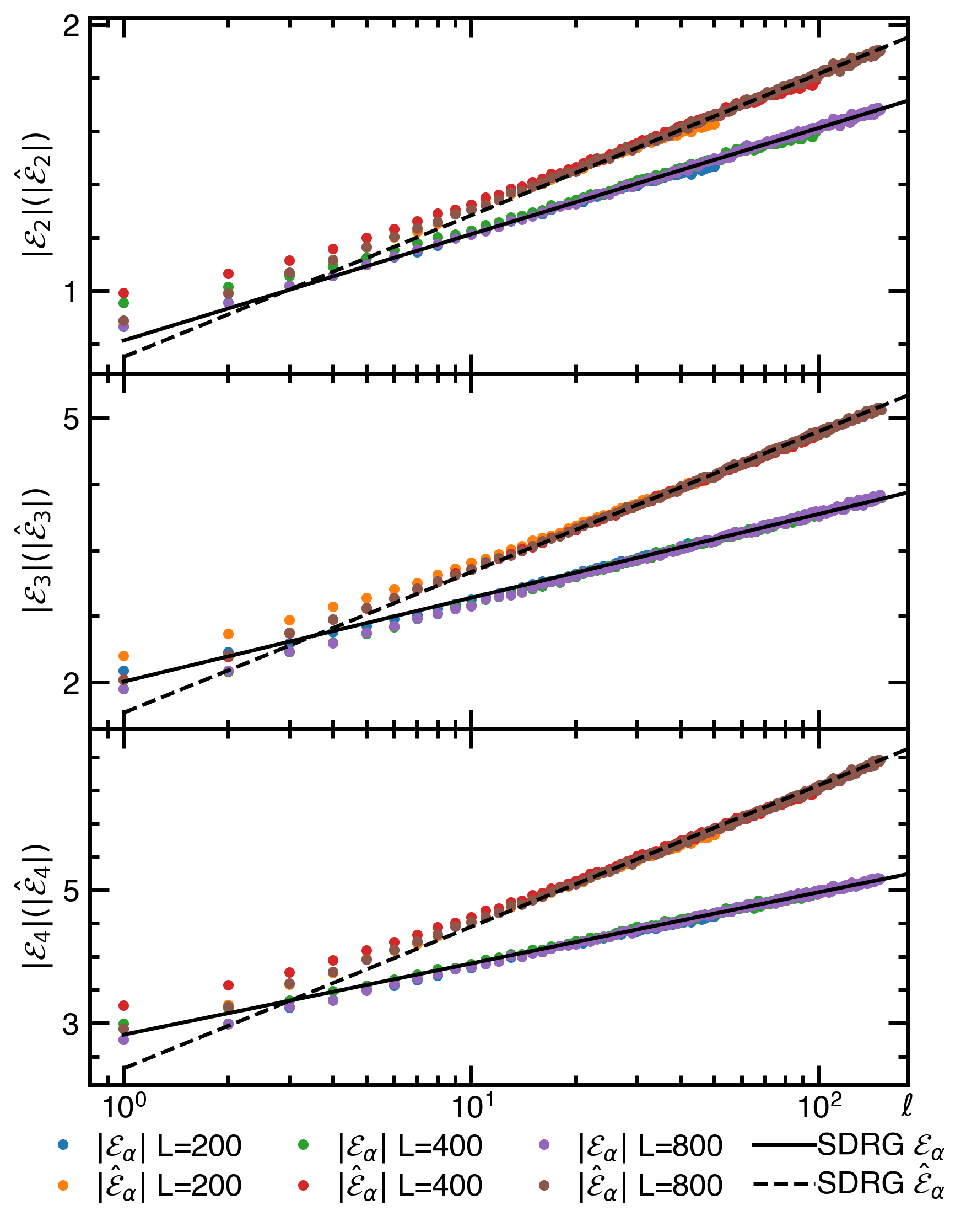
Figure 2: Negativity moments ${\cal E}_{\alpha}$ and $\hat{\cal E}_{\alpha}$ for the random XX chain: results of the ab initio computations for two adjacent intervals of equal length $\ell$. We report the absolute values, since for the considered values of $\alpha$, they are all negative quantities (i.e. the moments $M^{T_{2}}_{\alpha}$ are smaller than $1$). The symbols correspond to the numerical data while the continuous lines are the analytic SDRG predictions Eqs. (55-58), with a best fit for the unknown non-universal additive constants. The agreement between the simulation and SDRG predictions is excellent already for moderate values of $\ell$.

IV.2 Numerical results for adjacent intervals

We are finally ready to test numerically the predictions reported in Sec. III.4, as we do in the following. Throughout this section we consider a uniform coupling distribution ${P(J)=1}$ with ${J\in[0,1]}$, although, as stressed in Sec. II, the results are distribution independent because of the universality of the RSP. In order to perform the numerical calculations, we must consider a finite chain of length $L$ and, for simplicity, we choose to work with open boundary conditions. In order to reduce the finite size and boundary effects we take the two adjacent intervals placed at the center of the chain. We also limit our attention to the case of two intervals of equal length $\ell$, because all the universal factors may be extracted from this partition.

First we consider the ab-initio method for XX chain, reviewed in the previous subsection. We focus on $\alpha=2,3,4$. We consider different system sizes $L=200,400,800$ and we vary the intervals length $\ell$ between ${\ell\in\{1,\dots,L/4\}}$. We consider $10^{5}$ disorder realizations and we compute the disorder averages (31) and (32). The obtained numerical data are reported in Fig. 2. It is evident that all ${\cal E}_{\alpha}$ grow logarithmically with $\ell$ as predicted. The logarithmic growth is compared with the analytic predictions in Eqs. (55-58). The agreement between the numerical data and SDRG is perfect already for moderate values of $\ell$. In the plots the non-universal additive constants (not specified in Eqs. (55-58)) have been fitted.

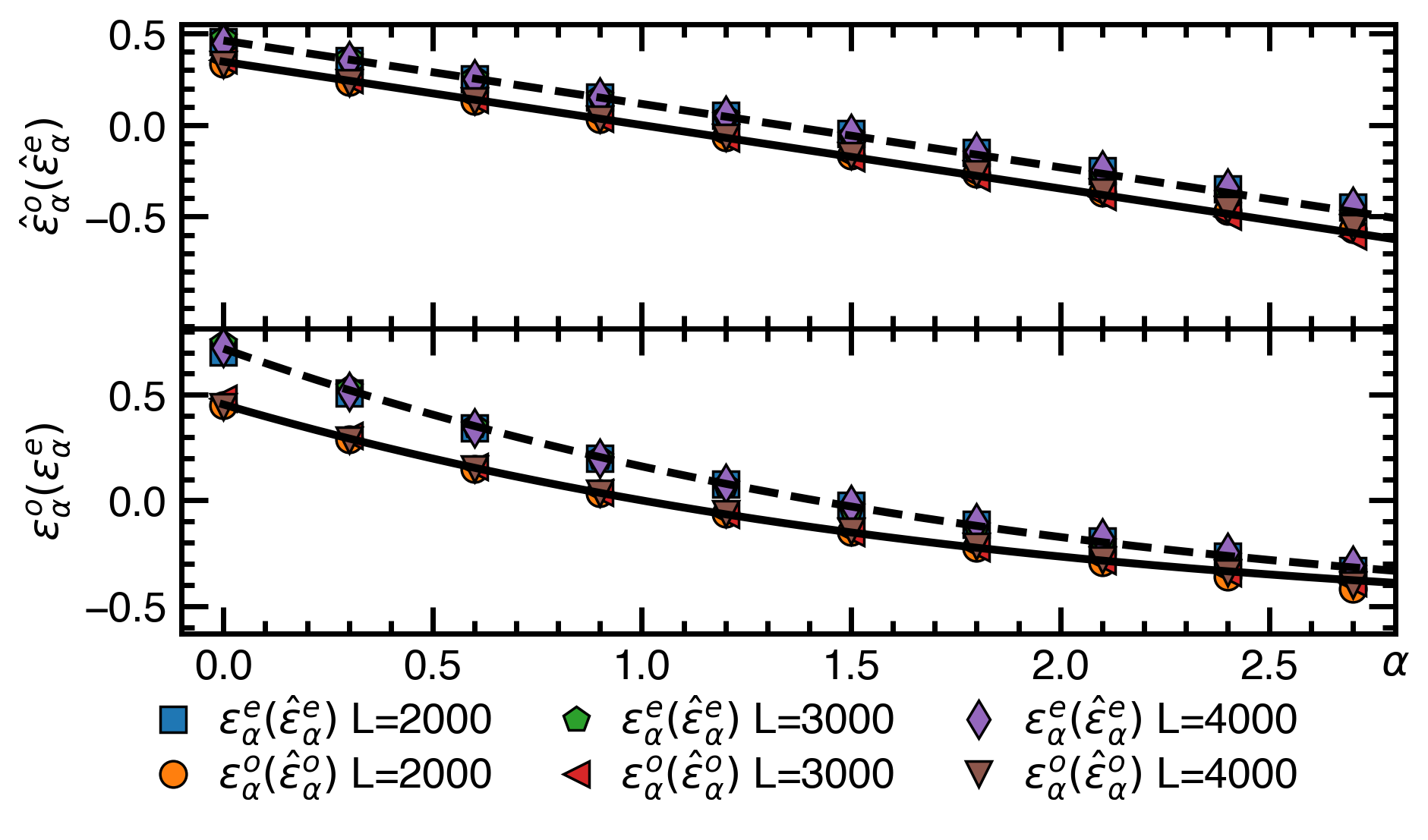
Figure 3: SDRG simulations for the negativity moments. Here we plot, as function of $\alpha$, the prefactor of the logarithm $\varepsilon^{e/o}_{\alpha}$ (cf. (81)), as obtained by a fit of the numerical data. The symbols are the corresponding numerical data while the continuous lines are the analytic predictions in Eqs. (55-58). The plots show an extremely good agreement between numerical data and analytic predictions.

A byproduct of these ab-initio numerical simulations is an indirect test of the SDRG scaling for the logarithmic negativity obtained in Ref. Ruggiero2016B, . In fact, the latter is not efficiently accessed through free fermion techniques, because, as already stressed many times, the partially transposed reduced density matrix is not a non-gaussian operator. Therefore, via replica trick, the computation of $\hat{\cal E}_{2\alpha}$ provides an indirect check for the scaling of the logarithmic negativity as well. This complement the numerical results obtained by SDRG and density matrix renormalization group in Ref. Ruggiero2016B, .

We now implement numerically the SDRG for finite spin chains, defined by the Ma-Dasgupta rule (11), which works as follows: (i) pick up a random disorder realization with a list random couplings ${J_{i}\sim P(J)}$; (ii) iterate the Ma-Dasgupta rule (i.e. choose the strongest bond, build a singlet between them, remove the two sites, renormalize the coupling according to (11)) until all spins are paired up in singlets; at each step keep track of the location of the singlet and of the removed spins; (iii) count the in-out singlets formed between the partitions of interest; (iv) evaluate the negativity moments for the single realization using their form in terms of the number of singlets in Eq. (30); (v) perform the average over all realizations. We vary the parameter $\alpha$, total length $L$, and the subsystem size $\ell$. Here the disorder average is taken over $10^{6}$ realizations. Since we are using Eq. (30) as operative definition of the negativity moments in the random singlet phase, we have direct access to the analytic continuations of all four families moments ${\cal E}^{e/o}_{\alpha}$ and $\hat{\cal E}^{e/o}_{\alpha}$ to even, odd and arbitrary non-integer values of $\alpha$. From these numerical averages, we extract the prefactor of the logarithm for all the negativity moments for several values of $\alpha$ fitting the averages with

$$\hat{\cal E}_{\alpha}^{e/o} = \hat{\varepsilon}_{\alpha}^{e/o}\log\ell+\hat{k}^{e/o}_{\alpha},$$ (81)

$${\cal E}_{\alpha}^{e/o} = \varepsilon_{\alpha}^{e/o}\log\ell+k^{e/o}_{\alpha}.$$

We restrict the fits to the windows of $\ell$ for which a logarithmic scaling is observed before finite size corrections kick in. The results for these four universal prefactors as function of $\alpha$ are reported in Fig. 3. The agreement between the analytic predictions in Eqs. (55-58) and the simulations is extremely good for the four moments and for all considered values of $\alpha$ (although some small finite size corrections are evident for the larger considered $\alpha$). These SDRG results provide a test not only for the integer negativity moments, but also for their analytical continuations (55-58).

V Conclusion

In this paper we exploited the Ma-Dasgupta decimation rule to write down a renewal equation for the probability distribution of in-out singlets in a tripartition of an infinite disordered spin chain in the random singlet phase. This procedure assumes that the most relevant renormalization effect is a single decimation occurring at a specific bond. The distribution resulting from the solution of the renewal equation provides analytic results for the negativity moments in the RSP and for their analytic continuations. We focused on the case of adjacent intervals and the results have been numerically tested by means of ab-initio simulations and numerical strong disorder renormalization group techniques, finding perfect agreement.

Our analysis naturally rises a few questions deserving further investigations. The first one is that the true negativity spectrum (i.e. the full distribution of eigenvalues of $\rho_{A}^{T_{2}}$) has not yet been derived. Indeed, this is still and open issue also for the entanglement spectrum Fagotti2011 for which the calculation should be much simpler. A second natural question is to wonder whether it is possible to calculate the negativity moments for other infinite randomness fixed points that have been described in the literature.

Finally, the dynamical evolution of the entanglement in random spin systems has been also subject to intensive investigation, especially in relation to many-body localized phases Serbyn13 ; Vosk2014 ; Altman15 ; Nandkishore15 ; Parameswaran2017 ; Abanin18 ; Pekker2014 ; Zhao2016 . A crucial aspect so far, even from the experimental side exp-lukin ; exp-mbl , has been to establish a quantitative understanding of the growth of the entanglement entropy. It would be interesting to generalize some of these results to the negativity and negativity spectrum.

Acknowledgement All authors acknowledge support from ERC: PC and PR under Consolidator grant number 771536 (NEMO) and XT under Starting grant number 758329 (AGEnTh).

Appendix A Fermionic negativity moments

The RSP describes also fermionic systems with random hoppings. However it has been shown was shown that the entanglement in the fermion variables is better captured by a fermionic negativity, introduced in Ref. ssr-17, and related to a partial time reversal operation. The associated spectrum has been studied for disorder-free fermions Hassan2019A . Therefore it is interesting to understand this spectrum in random systems and particularly in the RSP. In this appendix, we recall the definition of the two possible density matrices for fermionic negativity and determine them in the random singlet phase.

For interacting fermions, the hamiltonian is obtained from the XXZ hamiltonian (5), via a Jordan-Wigner trasformation

$$H=\sum_{j}J_{j}\left(c_{j}^{\dagger}c_{j+1}+c_{j+1}^{\dagger}c_{j}-\Delta n_{j}+\Delta n_{j}n_{j+1}\right),$$ (82)

where $c_{j},c_{j}^{\dagger}$ are spinless fermionic operators and ${n_{j}=c_{j}^{\dagger}c_{j}}$ the occupation number of the $j$-th site of the chain. The non-locality of such transformation points at a modification of the SDRG prescription to take into account the fermionic nature of the particles. It was shown sierra-fermions that this can be implemented through a simple modification of the RG prescription as

$$\tilde{J}=-\frac{J_{L}J_{R}}{\Omega}.$$ (83)

Eq. (83) implies that the hoppings can now be either positive or negative. When they are positive, a singlet-type bond is established between two sites, of the form ${|\psi_{-}\rangle\propto|01\rangle-|10\rangle}$, written in the occupation number basis of the fermions. If the hopping is negative, the corresponding triplet-type anti-bond is established ${|\psi_{+}\rangle\propto|01\rangle+|10\rangle}$. A crucial point is that the two types of bonds share many properties, such as entanglement. In particular, the spectrum of the associated density matrices is the same, ${\sigma(\rho_{+})=\sigma(\rho_{-})}$, where ${\rho_{\pm}=|\psi_{\pm}\rangle\langle\psi_{\pm}|}$. The same is true for the corresponding (standard) partial transpose, ${\sigma(\rho^{T_{2}}_{+})=\sigma(\rho^{T_{2}}_{-})}$. Therefore, for our purpose, the ground state in the RSP can be written as

$$|GS\rangle=\prod_{i}|\psi_{-}\rangle_{i}.$$ (84)

In the occupation number basis, the fermionic partial trasponse differs from the standard partial transpose just by a phase $e^{i\pi\phi}$, with

$$\phi(\{n_{j}\},\{\bar{n}_{j}\})=\frac{\tau_{1}(\tau_{1}+1)}{2}+\frac{\bar{\tau}_{1}(\bar{\tau}_{1}+1)}{2}+\tau_{2}\bar{\tau}_{2}\\ +\tau_{1}\tau_{2}+\bar{\tau}_{1}\bar{\tau}_{2}+(\tau_{1}+\tau_{2})(\bar{\tau}_{1}+\bar{\tau}_{2}).$$ (85)

Here ${\tau_{s}=\sum_{i\in A_{s}}n_{i}}$, ${\bar{\tau}=\sum_{i\in A_{s}}\bar{n}_{i}}$ and refer to the ket ${|\{n_{j}\}\rangle}$ and bra ${\langle\{\bar{n}_{j}\}|}$ state, respectively. See Ref. ssr-17, for details. In particular, applying the definition to our building block $\rho_{-}$, with the two subsystems consisting of a single site each, leads to

$$\rho_{-}^{R_{2}}= \frac{1}{2}\begin{pmatrix}0&0&0&-i\\ 0&1&0&0\\ 0&0&1&0\\ -i&0&0&0\end{pmatrix},$$ (86)

whose spectrum is given by ${\{i/2,-i/2,1/2,1/2\}}$.

We can now apply Eq. (86) to the reduced density matrix of the RSP, after tracing $B$, i.e.,

$$\rho_{A}=\bigotimes_{m=1}^{n_{A:A}}\rho_{\textup{2s}}\bigotimes_{n=1}^{n_{A:B}}\rho_{\textup{s}},$$

where here ${\rho_{\textup{2s}}=\rho_{-}}$ and ${\rho_{\textup{s}}=\textrm{tr}_{s}\rho_{-}}$ (with the trace being on one of the two sites). We obtain

$$\rho_{A}^{R_{2}}=\left\{\prod_{k=1,2}\bigotimes_{p=1}^{n_{A_{k}:A_{k}}}\rho_{\textup{2s}}\right\}\bigotimes_{q=1}^{n_{A_{1}:A_{2}}}\rho^{R_{2}}_{\textup{2s}}\left\{\prod_{k=1,2}\bigotimes_{r=1}^{n_{A_{k}:B}}\rho_{\textup{s}}\right\}.$$ (87)

Here we have used the fact that ${\rho_{\textup{s}}^{R_{2}}=\rho_{\textup{s}}}$ for a single site, and that ${\rho_{\textup{2s}}^{R_{2}}=\rho_{\textup{2s}}}$ when both the ends of a bond are in the same subsystem $A_{i}$ $(i=1,2)$.

There are 4 different non-zero eigenvalues

$$\lambda_{k}=2^{-n_{A:B}-n_{A_{1}:A_{2}}}e^{ik\pi/2},\;k=0,\pm 1,2.$$ (88)

These come with degeneracies $d_{k}$ given by

$$d_{\pm 1}=2^{n_{A:B}+n_{A_{1}:A_{2}}-2}\left(2^{n_{A_{1}:A_{2}}}\right),$$

$$d_{0}=2^{n_{A:B}+n_{A_{1}:A_{2}}-2}\left(2^{n_{A_{1}:A_{2}}}+2\right),$$ (89)

$$d_{2}=2^{n_{A:B}+n_{A_{1}:A_{2}}-2}\left(2^{n_{A_{1}:A_{2}}}-2\right).$$

From (88) and (A) we notice that the moments, ${M_{\alpha}^{R_{2}}\equiv\textrm{tr}\left(\rho_{A}^{R_{2}}\right)^{\alpha}}$ have three different analytic continuations when restricting to $\alpha$ integer

$$M_{\alpha}^{R_{2}}=2^{(n_{A:B}+n_{A_{1}:A_{2}})(1-\alpha)}\begin{cases}1\qquad\qquad&\alpha=2p+1,\\ 2^{n_{A_{1}:A_{2}}}\qquad&\alpha=4p,\\ 0\qquad\qquad&\alpha=4p+2,\\ \end{cases}$$ (90)

with $p$ integer. This more complicated periodicity has already been observed in the translational invariant setting Hassan2019A . As a check, from the odd sequence in (90) we recover the proper normalization ${\textrm{tr}\rho^{R_{2}}_{A}=\lim_{\alpha\to 1}M_{\alpha}^{R_{2}}=1}$.

This was dubbed untwisted negativity spectrum in Ref. Hassan2019A, , with the important difference with respect to the standard negativity spectrum of spin and bosonic models, of being complex. On the other hand, also for fermions one can introduce a hermitian partial transpose, more suitable to define another fermionic negativity due to its real spectrum. This is done by considering the composite operator ${\rho_{\times}\equiv(\rho^{R_{2}}_{A})^{\dagger}\rho^{R_{2}}_{A}}$ and by noting that ${\rho_{\times}=(\rho^{\tilde{R}_{2}}_{A})^{2}}$, where we introduced the twisted partial transpose ${\rho^{\tilde{R}_{2}}_{A}\equiv\rho_{A}^{R_{2}}(-1)^{F_{2}}}$ of Ref. Hassan2019A, . Here ${(-1)^{F_{2}}}$ is the fermion number parity in $A_{2}$, since ${F_{2}=\sum_{j\in A_{2}}n_{j}}$.

For the RSP, the twisted partial transposed reads

$$\rho_{A}^{\tilde{R}_{2}}=\left\{\prod_{k=1,2}\bigotimes_{p=1}^{n_{A_{k}:A_{k}}}\rho_{\textup{2s}}\right\}\bigotimes_{q=1}^{n_{A_{1}:A_{2}}}\rho^{\tilde{R}_{2}}_{\textup{2s}}\left\{\prod_{k=1,2}\bigotimes_{r=1}^{n_{A_{k}:B}}\rho_{\textup{s}}\right\}.$$ (91)

It has two non-zero eigenvalues

$$\tilde{\lambda}_{\pm}=\pm 2^{-n_{A:B}-n_{A_{1}:A_{2}}},$$ (92)

with equal degeneracy

$$\tilde{d}_{\pm}=2^{n_{A:B}+2n_{A_{1}:A_{2}}-1}.$$ (93)

Therefore, the associated moments, $M^{\tilde{R}_{2}}_{\alpha}\equiv\textrm{tr}\left(\rho^{\tilde{R}_{2}}_{A}\right)^{\alpha}$, are given by

$$M^{\tilde{R}_{2}}_{\alpha}=\begin{cases}0\hskip 119.50148pt\alpha\,\textrm{odd}\\ 2^{(n_{A:B}+n_{A_{1}:A_{2}})(1-\alpha)}2^{n_{A_{1}:A_{2}}}\quad\alpha\,\textrm{even}.\end{cases}$$ (94)

The negativity is obtained from Eq. (94) via replica limit as

$$\mathcal{E}=\lim_{\alpha\to 1/2}\overline{\log M_{2\alpha}^{\tilde{R}_{2}}}=\overline{n_{A_{1}:A_{2}}}\log 2.$$ (95)

Actually, in this case, Eq. (90) also implies that

$$\mathcal{E}=\lim_{\alpha\to 1/4}\overline{\log M_{4\alpha}^{{R}_{2}}}=\overline{n_{A_{1}:A_{2}}}\log 2.$$ (96)

Note that, as already shown numerically in Ref. ssr-17, , this means that in the case of fermions we recover the result obtained for the equivalent spin system in Ref. Ruggiero2016B, .

From Eqs. (90) and (94), it is clear that the fermionic negativity spectrum is different from the corresponding one in the spin variables. In fact, there are integer values of $\alpha$ for which they are trivial, i.e. are exactly vanishing. Nevertheless, the non-trivial moments have the same functional forms of the moments (30). As such, the same techniques employed in Section III may be used to obtain SDRG results for the disordered-average moments associated to twisted and untwisted density matrices. For example, within the same assumptions of Sec. III, the non-trivial untwisted moments reads

$$\log\overline{M_{\alpha}^{R_{2}}}=\begin{cases}\displaystyle\frac{\sqrt{5+2^{3-\alpha}}-3}{2}\mu+\dots\qquad\qquad&\alpha=2p+1,\\ \displaystyle\frac{\sqrt{5+(1+q)2^{3-\alpha}}-3}{2}\mu+\dots\qquad&\alpha=4p,\\ \end{cases}$$ (97)

while the non-trivial twisted ones are

$$\log\overline{M_{\alpha}^{\tilde{R}_{2}}}=\frac{\sqrt{5+(1+q)2^{3-\alpha}}-3}{2}\mu,\qquad\alpha\ \text{even}.$$ (98)

References

- (1) L. Amico, R. Fazio, A. Osterloh, and V. Vedral, Entanglement in many-body systems, Rev. Mod. Phys. 80, 517 (2008).
- (2) P. Calabrese, J. Cardy, and B. Doyon, Entanglement entropy in extended quantum systems, J. Phys. A 42, 500301 (2009).
- (3) N. Laflorencie, Quantum entanglement in condensed matter systems, Phys. Rep. 646, 1 (2016).
- (4) R. Islam, R. Ma, P. M. Preiss, M. E. Tai, A. Lukin, M. Rispoli, and M. Greiner, Measuring entanglement entropy in a quantum many-body system, Nature 528, 77 (2015).
- (5) H. Li and F. D. M. Haldane, Entanglement Spectrum as a Generalization of Entanglement Entropy: Identification of Topological Order in Non-Abelian Fractional Quantum Hall Effect States, Phys. Rev. Lett. 101, 010504 (2008).
- (6) N. Regnault, B. A. Bernevig and F. D. M. Haldane, Topological Entanglement and Clustering of Jain Hierarchy States, Phys. Rev. Lett. 103, 016801 (2009).
- (7) L. Fidkowski, Entanglement Spectrum of Topological Insulators and Superconductors, Phys. Rev. Lett. 104, 130502 (2010).
- (8) A. M. Läuchli, E. J. Bergholtz, J. Suorsa and M. Haque, Disentangling Entanglement Spectra of Fractional Quantum Hall States on Torus Geometries, Phys. Rev. Lett. 104, 156404 (2010).
- (9) H. Yao and X.-L. Qi, Entanglement Entropy and Entanglement Spectrum of the Kitaev Model, Phys. Rev. Lett. 105, 080501 (2010).
- (10) F. Pollmann, A. M. Turner, E. Berg and M. Oshikawa, Entanglement spectrum of a topological phase in one dimension, Phys. Rev. B 81, 064439 (2010).
- (11) J. Dubail and N. Read, Entanglement Spectra of Complex Paired Superfluids, Phys. Rev. Lett. 107, 157001 (2011).
- (12) X.-L. Qi, H. Katsura and A. W. W. Ludwig, General Relationship between the Entanglement Spectrum and the Edge State Spectrum of Topological Quantum States, Phys. Rev. Lett. 108, 196402 (2012).
- (13) D. Poilblanc, N. Schuch, D. Pérez-García and J. I. Cirac, Topological and entanglement properties of resonating valence bond wave functions, Phys. Rev. B 86, 014404 (2012).
- (14) L. Cincio and G. Vidal, Characterizing Topological Order by Studying the Ground States on an Infinite Cylinder, Phys. Rev. Lett. 110, 067208 (2013).
- (15) R. Lundgren, J. Blair, P. Laurell, N. Regnault, G.A. Fiete, M. Greiter and R. Thomale, Universal entanglement spectra in critical spin chains, Phys. Rev. B 94, 081112 (2016).
- (16) M. A. Metlitski and T. Grover, Entanglement Entropy of Systems with Spontaneously Broken Continuous Symmetry, arXiv:1112.5166 (2011).
- (17) V. Alba, M. Haque and A. M. Läuchli, Entanglement Spectrum of the Two-Dimensional Bose-Hubbard Model, Phys. Rev. Lett. 110, 260403 (2013).
- (18) F. Kolley, S. Depenbrock, I. P. McCulloch, U. Schollwöck and V. Alba, Entanglement spectroscopy of SU(2)-broken phases in two dimensions, Phys. Rev. B 88, 144426 (2013).
- (19) N. M. Tubman and D. C. Yang, Calculating the entanglement spectrum in quantum Monte Carlo with application to ab initio Hamiltonians, Phys. Rev. B 90, 081116 (2014).
- (20) I. Frérot and T. Roscilde, Entanglement Entropy across the Superfluid-Insulator Transition: A Signature of Bosonic Criticality, Phys. Rev. Lett. 116, 190401 (2016).
- (21) Z.-C. Yang, C. Chamon, A. Hamma and E. R. Mucciolo, Two-Component Structure in the Entanglement Spectrum of Highly Excited States, Phys. Rev. Lett. 115, 267206 (2015).
- (22) S. D. Geraedts, R. Nandkishore and N. Regnault, Many-body localization and thermalization: Insights from the entanglement spectrum, Phys. Rev. B 93, 174202 (2016).
- (23) M. Serbyn, A. A. Michailidis, D. A. Abanin and Z. Papic, Power-Law Entanglement Spectrum in Many-Body Localized Phases, Phys. Rev. Lett. 117, 160601 (2016).
- (24) P. Calabrese and A. Lefevre, Entanglement spectrum in one-dimensional systems, Phys. Rev. A 78, 032329 (2008).
- (25) F. Pollmann and J. E. Moore, Entanglement spectra of critical and near-critical systems in one dimension, New J. Phys. 12, 025006 (2010).
- (26) A. M. Läuchli, Operator content of real-space entanglement spectra at conformal critical points, arXiv:1303.0741 (2013).
- (27) Y.O. Nakagawa and S. Furukawa, Capacity of entanglement and distribution of density matrix eigenvalues in gapless systems, Phys. Rev. B 96, 205108 (2017).
- (28) M. Goldstein and E. Sela, Symmetry-Resolved Entanglement in Many-Body Systems, Phys. Rev. Lett. 120, 200602 (2018).
- (29) V. Alba, P. Calabrese and E. Tonni, Entanglement spectrum degeneracy and the Cardy formula in 1+1 dimensional conformal field theories, J. Phys. A 51, 024001 (2018).
- (30) L. Tagliacozzo, T. R. de Oliveira, S. Iblisdir and J. I. Latorre, Scaling of entanglement support for matrix product states, Phys. Rev. B 78, 024410 (2008).
- (31) F. Pollmann, S. Mukerjee, A. M. Turner and J. E. Moore, Theory of Finite-Entanglement Scaling at One-Dimensional Quantum Critical Points, Phys. Rev. Lett. 102, 255701 (2009).
- (32) B. Pirvu, G. Vidal, F. Verstraete and L. Tagliacozzo, Matrix product states for critical spin chains: Finite-size versus finite-entanglement scaling, Phys. Rev. B 86, 075117 (2012).
- (33) A. Peres, Separability Criterion for Density Matrices, Phys. Rev. Lett. 77, 1413 (1996).
- (34) M. Horodecki, P. Horodecki and R. Horodecki, Separability of mixed states: necessary and sufficient conditions, Phys. Lett. A 223, 1 (1996).
- (35) R. Simon, Peres-Horodecki Separability Criterion for Continuous Variable Systems, Phys. Rev. Lett. 84, 2726 (2000).
- (36) R. F. Werner and M. M. Wolf, Bound Entangled Gaussian States, Phys. Rev. Lett. 86, 3658 (2001).
- (37) G. Giedke, B. Kraus, M. Lewenstein and J. I. Cirac, Entanglement Criteria for All Bipartite Gaussian States, Phys. Rev. Lett. 87, 167904 (2001).
- (38) K Zyczkowski, P. Horodecki, A. Sanpera, and M. Lewenstein, Volume of the set of separable states, Phys. Rev. A 58, 883 (1998).
- (39) K Zyczkowski, Volume of the set of separable states. II, Phys. Rev. A 60, 3496 (1999).
- (40) J. Eisert and M. B. Plenio, A comparison of entanglement measures, J. Mod. Opt. 46, 145 (1999).
- (41) J. Lee, M. S. Kim, Y. J. Park, and S. Lee, Partial teleportation of entanglement in a noisy environment, J. Mod. Opt. 47, 2151 (2000).
- (42) G. Vidal and R. F. Werner, Computable measure of entanglement, Phys. Rev. A 65, 032314 (2002).
- (43) M. B. Plenio, Logarithmic Negativity: A Full Entanglement Monotone That is not Convex, Phys. Rev. Lett. 95, 090503 (2005).
- (44) K. Audenaert, J. Eisert, M. B. Plenio and R. F. Werner, Entanglement properties of the harmonic chain, Phys. Rev. A 66, 042327 (2002).
- (45) A. Ferraro, D. Cavalcanti, A. García-Saez and A. Acín, Thermal Bound Entanglement in Macroscopic Systems and Area Law, Phys. Rev. Lett. 100, 080502 (2008).
- (46) D. Cavalcanti, A. Ferraro, A. García-Saez and A. Acín, Distillable entanglement and area laws in spin and harmonic-oscillator systems, Phys. Rev. A 78, 012335 (2008).
- (47) J. Anders and W. Andreas, Entanglement and separability of quantum harmonic oscillator systems at finite temperature, Quantum Info. Comput. 8, 0245 (2008).
- (48) J. Anders, Thermal state entanglement in harmonic lattices, Phys. Rev. A 77, 062102 (2008).
- (49) S. Marcovitch, A. Retzker, M. B. Plenio and B. Reznik, Critical and noncritical long-range entanglement in Klein-Gordon fields, Phys. Rev. A 80, 012325 (2009).
- (50) N. E. Sherman, T. Devakul, M. B. Hastings and R. R. P. Singh, Nonzero-temperature entanglement negativity of quantum spin models: Area law, linked cluster expansions, and sudden death, Phys. Rev. E 93, 022128 (2016).
- (51) C. D. Nobili, A. Coser and E. Tonni, Entanglement negativity in a two dimensional harmonic lattice: area law and corner contributions, J. Stat. Mech. 083102 (2016).
- (52) V. Eisler and Z. Zimboras, Entanglement negativity in two-dimensional free lattice models, Phys. Rev. B 93, 115148 (2016).
- (53) M R. M. Mozaffar and A. Mollabashi, Logarithmic negativity in Lifshitz harmonic models, J. Stat. Mech. (2018) 053113.
- (54) H. Wichterich, J. Molina-Vilaplana and S. Bose, Scaling of entanglement between separated blocks in spin chains at criticality, Phys. Rev. A 80, 010304 (2009).
- (55) A. Bayat, S. Bose and P. Sodano, Entanglement Routers Using Macroscopic Singlets, Phys. Rev. Lett. 105, 187204 (2010).
- (56) A. Bayat, P. Sodano and S. Bose, Negativity as the entanglement measure to probe the Kondo regime in the spin-chain Kondo model, Phys. Rev. B 81, 064429 (2010).
- (57) A. Bayat, S. Bose, P. Sodano and H. Johannesson, Entanglement Probe of Two-Impurity Kondo Physics in a Spin Chain, Phys. Rev. Lett. 109, 066403 (2012).
- (58) H. Wichterich, J. Vidal and S. Bose, Universality of the negativity in the Lipkin-Meshkov-Glick model, Phys. Rev. A 81, 032311 (2010).
- (59) R. A. Santos, V. Korepin and S. Bose, Negativity for two blocks in the one-dimensional spin-1 Affleck-Kennedy-Lieb-Tasaki model, Phys. Rev. A 84, 062307 (2011).
- (60) N. E. Sherman, T. Devakul, M. B. Hastings, and R. R. P. Singh, Nonzero-temperature entanglement negativity of quantum spin models: Area law, linked cluster expansions, and sudden death, Phys. Rev. E 93, 022128 (2016).
- (61) T.-C. Lu and T. Grover, Singularity in Entanglement Negativity Across Finite Temperature Phase Transitions, arXiv:1808.04381 (2018).
- (62) Y. Javanmard, D. Trapin, S. Bera, J. H. Bardarson and M. Heyl, Sharp entanglement thresholds in the logarithmic negativity of disjoint blocks in the transverse-field Ising chain, New J. Phys. 20, 083032 (2018).
- (63) J. Gray, A. Bayat, A. Pal, and S. Bose, Scale Invariant Entanglement Negativity at the Many-Body Localization Transition, ArXiv:1908.02761.
- (64) J. Kudler-Flam, H. Shapourian, and S. Ryu, The negativity contour: a quasi-local measure of entanglement for mixed states, ArXiv:1908.07540.
- (65) E. Cornfeld, M. Goldstein, and E. Sela, Imbalance entanglement: Symmetry decomposition of negativity, Phys. Rev. A 98, 032302 (2018).
- (66) P. Calabrese, J. Cardy and E. Tonni, Entanglement Negativity in Quantum Field Theory, Phys. Rev. Lett. 109, 130502 (2012).
- (67) P. Calabrese, J. Cardy and E. Tonni, Entanglement negativity in extended systems: a field theoretical approach, J. Stat. Mech. P02008 (2013).
- (68) P. Calabrese, L. Tagliacozzo and E. Tonni, Entanglement negativity in the critical Ising chain, J. Stat. Mech. P05002 (2013).
- (69) V. Alba, Entanglement negativity and conformal field theory: a Monte Carlo study, J. Stat. Mech. P05013 (2013).
- (70) P. Calabrese, J. Cardy and E. Tonni, Finite temperature entanglement negativity in conformal field theory, J. Phys. A 48, 015006 (2015).
- (71) C. D. Nobili, A. Coser and E. Tonni, Entanglement entropy and negativity of disjoint intervals in CFT: some numerical extrapolations, J. Stat. Mech. P06021 (2015).
- (72) M. Kulaxizi, A. Parnachev and G. Policastro, Conformal blocks and negativity at large central charge, JHEP 09 (2014) 010.
- (73) O. Blondeau-Fournier, O. A. Castro-Alvaredo and B. Doyon, Universal scaling of the logarithmic negativity in massive quantum field theory, J. Phys. A 49, 125401 (2016).
- (74) D. Bianchini and O. A. Castro-Alvaredo, Branch point twist field correlators in the massive free Boson theory, Nuc. Phys. B 913, 879 (2016).
- (75) A. Coser, E. Tonni and P. Calabrese, Entanglement negativity after a global quantum quench, J. Stat. Mech. P12017 (2014).
- (76) V. Eisler and Z. Zimborás, Entanglement negativity in the harmonic chain out of equilibrium, New J. Phys. 16, 123020 (2014).
- (77) M. Hoogeveen and B. Doyon, Entanglement negativity and entropy in non-equilibrium conformal field theory, Nuc. Phys. B 898, 78 (2015).
- (78) X. Wen, P.-Y. Chang and S. Ryu, Entanglement negativity after a local quantum quench in conformal field theories, Phys. Rev. B 92, 075109 (2015).
- (79) V. Alba and P. Calabrese, Quantum information dynamics in multipartite integrable systems, EPL 126, 60001 (2019).
- (80) M. J. Gullans and D. A. Huse, Entanglement Structure of Current-Driven Diffusive Fermion Systems, Phys. Rev. X 9, 021007 (2019).
- (81) J. Kudler-Flam, M. Nozaki, S. Ryu, and M. T. Tan, Quantum vs. classical information: operator negativity as a probe of scrambling, arXiv:1906.07639.
- (82) X. Wen, S. Matsuura and S. Ryu, Edge theory approach to topological entanglement entropy, mutual information, and entanglement negativity in Chern-Simons theories, Phys. Rev. B 93, 245140 (2016).
- (83) X. Wen, P.-Y. Chang and S. Ryu, Topological entanglement negativity in Chern-Simons theories, JHEP 09, 012 (2016).
- (84) C. Castelnovo, Negativity and topological order in the toric code, Phys. Rev. A 88, 042319 (2013).
- (85) Y. A. Lee and G. Vidal, Entanglement negativity and topological order, Phys. Rev. A 88, 042318 (2013).
- (86) O. Hart and C. Castelnovo, Entanglement negativity and sudden death in the toric code at finite temperature, Phys. Rev. B 97, 144410 (2018).
- (87) F. Pollmann and A. M. Turner, Detection of symmetry-protected topological phases in one dimension, Phys. Rev. B 86, 125441 (2012).
- (88) K. Shiozaki and S. Ryu, Matrix product states and equivariant topological field theories for bosonic symmetry-protected topological phases in (1+1) dimensions, JHEP 04, 100 (2017).
- (89) H. Shapourian, K. Shiozaki and S. Ryu, Many-Body Topological Invariants for Fermionic Symmetry-Protected Topological Phases, Phys. Rev. Lett. 118, 216402 (2017).
- (90) K. Shiozaki, H. Shapourian, K. Gomi and S. Ryu, Many-body topological invariants for fermionic short-range entangled topological phases protected by antiunitary symmetries, Phys. Rev. B 98, 035151 (2018).
- (91) V. Eisler and Z. Zimboras, On the partial transpose of fermionic Gaussian states, New J. Phys. 17, 053048 (2015).
- (92) C. P. Herzog and Y. Wang, Estimation for entanglement negativity of free fermions, J. Stat. Mech. 073102 (2016).
- (93) J. Eisert, V. Eisler and Z. Zimborás, Entanglement negativity bounds for fermionic Gaussian states, Phys. Rev. B 97, 165123 (2018).
- (94) A. Coser, E. Tonni and P. Calabrese, Towards the entanglement negativity of two disjoint intervals for a one dimensional free fermion, J. Stat. Mech. 033116 (2016).
- (95) P.-Y. Chang and X. Wen, Entanglement negativity in free-fermion systems: An overlap matrix approach, Phys. Rev. B 93, 195140 (2016).
- (96) H. Shapourian, K. Shiozaki and S. Ryu, Partial time-reversal transformation and entanglement negativity in fermionic systems, Phys. Rev. B 95, 165101 (2017).
- (97) H. Shapourian and S. Ryu, Entanglement negativity of fermions: Monotonicity, Separability criterion, and classification of few-mode states, Phys. Rev. A 99, 022310 (2019).
- (98) H. Shapourian and S. Ryu, Finite-temperature entanglement negativity of free fermions, J. Stat. Mech. (2019) 043106.
- (99) J. Gray, L. Banchi, A. Bayat and S. Bose, Machine-Learning-Assisted Many-Body Entanglement Measurement, Phys. Rev. Lett. 121, 150503 (2018).
- (100) E. Cornfeld, E. Sela and M. Goldstein, Measuring Fermionic Entanglement: Entropy, Negativity, and Spin Structure, Phys. Rev. A 99, 062309 (2019).
- (101) P. Ruggiero, V. Alba and P. Calabrese, Negativity spectrum of one-dimensional conformal field theories, Phys. Rev. B 94, 195121 (2016).
- (102) G. B. Mbeng, V. Alba and P. Calabrese, Negativity spectrum in 1D gapped phases of matter, J. Phys. A 50, 194001 (2017).
- (103) H. Shapourian, P. Ruggiero, S. Ryu, and P. Calabrese, Twisted and untwisted negativity spectrum of free fermions, arxiv:1906.04211 (2019).
- (104) P.W. Anderson, Absence of Diffusion in Certain Random Lattices, Phys. Rev. 109, 1492 (1958).
- (105) E. Abrahams, 50 Years of Anderson Localization, World Scientific (2010).
- (106) R. Nandkishore and D. A. Huse, Many body localization and thermalization in quantum statistical mechanics, Ann. Review of Cond. Mat. Phys. 6, 15 (2015).
- (107) D.A. Abanin, E. Altman, I. Bloch, and M. Serbyn Colloquium: Many-body localization, thermalization, and entanglement, Rev. Mod. Phys. 91, 021001 (2019).
- (108) S.-K. Ma, C. Dasgupta, and C.-k. Hu, Random Antiferromagnetic Chain, Phys. Rev. Lett. 43, 1434 (1979).
- (109) C. Dasgupta and S.-K. Ma, Low-temperature properties of the random Heisenberg antiferromagnetic chain, Phys. Rev. B 22, 1305 (1980).
- (110) D. S. Fisher, Random transverse field Ising spin chains, Phys. Rev. Lett. 69, 534 (1992).
- (111) D. S. Fisher, Critical behavior of random transverse-field Ising spin chains, Phys. Rev. B 51, 6411 (1995).
- (112) F. Iglói and C. Monthus, Strong disorder RG approach of random systems, Phys. Rep. 412, 277 (2005).
- (113) F. Igloi and C. Monthus Strong Disorder RG approach - a short review of recent developments, Eur. Phys. J. B 91, 290 (2018).
- (114) G. Refael and J. E. Moore, Criticality and entanglement in random quantum systems, J. Phys. A 42, 504010 (2009).
- (115) G. Refael and J. E. Moore, Entanglement Entropy of Random Quantum Critical Points in One Dimension, Phys. Rev. Lett. 93, 260602 (2004).
- (116) N. Laflorencie, Scaling of entanglement entropy in the random singlet phase, Phys. Rev. B 72, 140408(R) (2005).
- (117) G. De Chiara, S. Montangero, P. Calabrese, and R. Fazio, Entanglement entropy dynamics of Heisenberg chains, J. Stat. Mech. P03001 (2006).
- (118) L. Fidkowski, G. Refael, N. E. Bonesteel, and J. E. Moore, c-theorem violation for effective central charge of infinite-randomness fixed points Phys. Rev. B 78, 224204 (2008).
- (119) R. Santachiara, Increasing of entanglement entropy from pure to random quantum critical chains, J. Stat. Mech. L06002 (2006).
- (120) G. Refael and J. E. Moore, Entanglement entropy of the random s=1 Heisenberg chain Phys. Rev. B 76, 024419 (2007).
- (121) J. A. Hoyos, A. P. Vieira, N. Laflorencie, and E. Miranda, Correlation amplitude and entanglement entropy in random spin chains, Phys. Rev. B 76, 174425 (2007).
- (122) Y.-C. Lin, F. Igloi, and H. Rieger, Entanglement Entropy at Infinite-Randomness Fixed Points in Higher Dimensions, Phys. Rev. Lett. 99, 147202 (2007).
- (123) N. E. Bonesteel and K. Yang, Infinite-Randomness Fixed Points for Chains of Non-Abelian Quasiparticles, Phys. Rev. Lett. 99, 140405 (2007).
- (124) D. Binosi, G. De Chiara, S. Montangero, and A. Recati, Increasing entanglement through engineered disorder in the random Ising chain, Phys. Rev. B 76, 140405 (2007).
- (125) F. Igloi and Y.-C. Lin, Finite-size scaling of the entanglement entropy of the quantum Ising chain with homogeneous, periodically modulated and random couplings, J. Stat. Mech. P06004 (2008).
- (126) R. Yu, H. Saleur, and S. Haas, Entanglement entropy in the two-dimensional random transverse field Ising model, Phys. Rev. B 77, 140402 (2008).
- (127) J. A. Hoyos, N. Laflorencie, A. P. Vieira, and T. Vojta, Protecting clean critical points by local disorder correlations, Europhys. Lett. 93, 30004 (2011).
- (128) I. A. Kovacs, and F. Igloi, Critical behavior and entanglement of the random transverse-field Ising model between one and two dimensions, Phys. Rev. B 80, 214416 (2009).
- (129) I. A. Kovacs, and F. Igloi, Universal logarithmic terms in the entanglement entropy of 2d, 3d and 4d random transverse-field Ising models, Europhys. Lett 97, 67009 (2012).
- (130) J. C. Getelina, F. C. Alcaraz, and J. A. Hoyos, Entanglement properties of correlated random spin chains and similarities with conformally invariant systems, Phys. Rev. B 93, 045136 (2016).
- (131) J. Rodriguez-Laguna, S. N. Santalla, G. Ramirez, and G. Sierra, Entanglement in correlated random spin chains, RNA folding and kinetic roughening, New J. Phys. 18, 073025 (2016).
- (132) C. K. Burrell and T. J. Osborne, Bounds on the Speed of Information Propagation in Disordered Quantum Spin Chains, Phys. Rev. Lett. 99, 167201 (2007).
- (133) F. Igloi, Z. Szatmari, and Y.-C. Lin, Entanglement entropy dynamics of disordered quantum spin chains, Phys. Rev. B 85, 094417 (2012).
- (134) J. H. Bardarson, F. Pollmann, and J. E. Moore, Unbounded Growth of Entanglement in Models of Many-Body Localization, Phys. Rev. Lett. 109, 017202 (2012).
- (135) V. Alba, S. N. Santalla, P. Ruggiero, J. Rodriguez-Laguna, P. Calabrese, and G. Sierra, Unusual area-law violation in random inhomogeneous systems, J. Stat. Mech. (2019) 023105.
- (136) S. Pappalardi, P. Calabrese, and G. Parisi, Entanglement entropy of the long-range Dyson hierarchical model, J. Stat. Mech. (2019) 073102.
- (137) P. Ruggiero, V. Alba and P. Calabrese, Entanglement negativity in random spin chains, Phys. Rev. B 94, 035152 (2016).
- (138) M. Pouranvari and K. Yang, Entanglement spectrum and entangled modes of random XX spin chains, Phys. Rev. B 88, 075123 (2013).
- (139) G. Torlai, K. D. McAlpine, and G. De Chiara, Schmidt gap in random spin chains, Phys. Rev. B 98, 085153 (2018).
- (140) M. Fagotti, P. Calabrese and J. E. Moore, Entanglement spectrum of random-singlet quantum critical points, Phys. Rev. B 83, 045110 (2011).
- (141) G. Ramirez, J. Rodriguez-Laguna, and G. Sierra, Entanglement in low-energy states of the random-hopping model, J. Stat. Mech. P07003 (2014).
- (142) J. Cardy, Scaling and Renormalization in Statistical Physics, CUP, Cambridge, UK (2015),
- (143) D. Fisher, Random antiferromagnetic quantum spin chains, Phys. Rev. B 50, 3799 (1994).
- (144) R. Vasseur and J.E. Moore, Multifractal orthogonality catastrophe in one-dimensional random quantum critical points, Phys. Rev. B 92, 054203 (2015).
- (145) M. Fagotti and P. Calabrese, Entanglement entropy of two disjoint blocks in XY chains, J. Stat. Mech. P04016 (2010).
- (146) A. Coser, E. Tonni and P. Calabrese, Partial transpose of two disjoint blocks in XY spin chains, J. Stat. Mech. P08005 (2015).
- (147) R. Balian and E. Brezin, Nonunitary Bogoliubov transformations and extension of Wick’s theorem, Il Nuovo Cimento B 64, 37 (1969).
- (148) I. Peschel and V. Eisler, Reduced density matrices and entanglement entropy in free lattice models, J. Phys. A 42, 504003 (2009).
- (149) V. Alba, L. Tagliacozzo, and P. Calabrese, Entanglement entropy of two disjoint blocks in critical Ising models, Phys. Rev. B 81, 060411 (2010).
- (150) F. Igloi and I. Peschel, On reduced density matrices for disjoint subsystems, EPL 89, 40001 (2010).
- (151) J. Zhang, P. Ruggiero, and P. Calabrese, Subsystem trace distance in low-lying states of (1+1)-dimensional conformal field theories, arXiv:1907.04332 (2019).
- (152) M. Serbyn, Z. Papic, and D. A. Abanin, Universal Slow Growth of Entanglement in Interacting Strongly Disordered Systems, Phys. Rev. Lett. 110, 260601 (2013).
- (153) R. Vosk and E. Altman, Dynamical Quantum Phase Transitions in Random Spin Chains, Phys. Rev. Lett. 112, 217204 (2014).
- (154) E. Altman and R. Vosk, Universal dynamics and renormalization in many body localized systems, Ann. Review of Cond. Mat. Phys. 6, 383 (2015).
- (155) S. A. Parameswaran, A. C. Potter and R. Vasseur, Eigenstate phase transitions and the emergence of universal dynamics in highly excited states, Annalen der Physik 529, 1600302 (2017).
- (156) D. A. Abanin, E. Altman, I. Bloch and M. Serbyn, Ergodicity, Entanglement and Many-Body Localization, Rev. Mod. Phys. 91, 021001 (2019)
- (157) D. Pekker, G. Refael, E. Altman, E. Demler, and V. Oganesyan, Hilbert-Glass Transition: New Universality of Temperature-Tuned Many-Body Dynamical Quantum Criticality, Phys. Rev. X 4, 011052 (2014).
- (158) Y. Zhao, F. Andraschko, and J. Sirker, Entanglement entropy of disordered quantum chains following a global quench, Phys. Rev. B 93, 205146 (2016).
- (159) A. Lukin, M. Rispoli, R. Schittko, M. E. Tai, A. M. Kaufman, S. Choi, V. Khemani, J. Leonard, and M. Greiner, Probing entanglement in a many-body localized system, Science 364, 6437 (2019).
- (160) B. Chiaro et. al., Growth and preservation of entanglement in a many-body localized system, arXiv:1910.06024.
- (161) G. Ramirez, J. Rodriguez-Laguna and G. Sierra, Entanglement over the rainbow, J. Stat. Mech. (2015) P06002