The large-separation expansion of peak clustering in Gaussian random fields

Abstract

In the peaks approach, the formation sites of observable structures in the Universe are identified as peaks in the matter density field. The statistical properties of the clustering of peaks are particularly important in this respect. In this paper, we investigate the large-separation expansion of the correlation function of peaks in Gaussian random fields. The analytic formula up to third order is derived, and the resultant expression can be evaluated by a combination of one-dimensional fast Fourier transforms, which are evaluated very fast. The analytic formula obtained perturbatively in the large-separation limit is compared with a method of Monte-Carlo integrations, and a complementarity between the two methods is demonstrated.

I Introduction

All the cosmological structures in the Universe emerge from initial density fluctuations in the early Universe bkp . The formation of astronomical objects is a complicated process, including nonlinear dynamics, baryonic physics, radiative transfer, etc., and the relation between the formation sites of astronomical objects and the spatial distribution of matter is also complicated in general, the astronomical objects being biased tracers of the total matter distribution in the Universe (for a review, see Ref. DJS18 ). Modelling this bias relation is one of the key problems in the context of large-scale structure of the Universe, especially with the advent of high precision cosmological surveys such as Euclid, LSST, WFIRST to name a few, which require a detailed modelling of galaxy bias, flexible and accurate enough not to bias the resulting cosmological constraints krause16 – notably on dark energy, the ultimate goal of these experiments.

In the peak approach, the formation of dark matter halos is assumed to take place at the density peaks of the initial density field in Lagrangian space Dor70 ; Kai84 ; PH85 ; BBKS . Although this assumption is oversimplified, there are empirical evidences that massive halos corresponds to the high-density peaks in Lagrangian space FWDE88 ; WMS94 ; Lud11 .

The peak approach can explain the clustering amplitude of rich clusters, which is much higher than that of galaxies. Indeed, it was shown that the high-density rare peaks in the Gaussian random field are more strongly clustered than the underlying (mass) density field Kai84 , an effect known as peak bias. Since then, the clustering properties of peaks in Gaussian random fields have attracted much attention BBKS ; PW84 ; Ott86 ; Cli87 ; Cat88 ; LHP89 ; Col89 ; RS95 ; Mat95 . The biasing by peaks has interesting properties which are not present in a simple model of local bias. The higher-derivatives of the underlying density field in the peak formalism affect the scale of baryon acoustic oscillations Des08 ; DCSS10 , and predict interplay between bias and gravitational evolution Bal15 . A combination of the peak approach and the excursion-set approach was also proposed AP90 ; PS12 ; PSD13 ; BCDP14 to improve the modelling of the mass function of dark matter halos.

The evaluation of the correlation function of peaks in the Gaussian random fields is one of the essential problems in the peak approach. One can write down an analytic expression for the peak correlation function in the Gaussian random field, which is represented by 14-dimensional integrals RS95 . It is possible to adopt Monte-Carlo integrations to numerically evaluate such integrals at the price of a large computational cost, as was done in BCDP16 for peaks in 1D and in CPP18 in 3D to predict the connectivity of the cosmic web. Instead, the correlation function of peaks on large scales can be evaluated by applying an orthogonal expansion of peaks Sza88 ; Col93 ; Mat95 ; LMD16 ; Diz16 . The orthogonal expansion method of the Lagrangian bias in Refs. Mat95 ; LMD16 is closely related to the formalism of integrated Perturbation Theory (iPT) Mat11 ; Mat12 ; Mat14 ; MD16 . In fact, the functional coefficients of the orthogonal expansion are the same as the renormalized bias functions in terms of iPT for Gaussian initial conditions. These expansion methods correspond to the large-separation expansion, because the expansion series are accurate when the correlation function of the underlying density field is small enough.

In this paper, we explicitly derive analytic formulas for the large-separation expansion up to third order. While primary expressions are given with multi-dimensional integrals in Fourier space, they reduce to combination of one-dimensional Fast Fourier Transforms (FFTs) in configuration space, applying a technique developed by Refs. SVM16 ; SV16 ; MFHB16 ; FBMH17 . The results are compared with a Monte-Carlo integration of the full expression of the peak correlation function.

The paper is organized as follows. We briefly review the peak approach in Sec. II. In Sec. III, a detailed method to derive the formula for the large-separation expansion is described, and the formula up to third order is explicitly given. In the course of the derivation, useful equations to evaluate the bias coefficients of peaks are presented. In Sec. IV, a simple calculation with a cosmological density field is given, and the result is compared with a Monte-Carlo integration method. Finally, conclusions are given in Sec. V.

II Basics of peak theory

II.1 Field variables and Gaussian statistics

In this section, we review some basic results of peak theory. For a given density contrast $\delta(\bm{x})$, a smoothed density contrast is given by

$$\delta_{\mathrm{s}}(\bm{x})=\int d^{3}x^{\prime}W_{R}(|\bm{x}-\bm{x}^{\prime}|)\,\delta(\bm{x}^{\prime}),$$ (1)

where $W_{R}(x)$ is a smoothing kernel, and $R$ is a smoothing radius. The Fourier transform of the above equation is given by

$$\tilde{\delta}_{\mathrm{s}}(\bm{k})=W(kR)\,\tilde{\delta}(\bm{k}),$$ (2)

where $\tilde{\delta}_{\mathrm{s}}(\bm{k})$ and $W(kR)$ are (3-dimensional) Fourier transforms of $\delta_{\mathrm{s}}(\bm{x})$ and $W_{R}(\bm{x})$ respectively. A common choice for the smoothing kernel is a Gaussian window, $W(kR)=e^{-k^{2}R^{2}/2}$. However, we do not assume any specific form for the kernel function in this paper, as long as it filters high-frequency modes.

The power spectrum $P(k)$ of the underlying density field is given by

$$\left\langle\tilde{\delta}(\bm{k})\,\tilde{\delta}(\bm{k}^{\prime})\right\rangle=(2\pi)^{3}\delta_{\mathrm{D}}^{3}(\bm{k}+\bm{k}^{\prime})\,P(k),$$ (3)

and the power spectrum of the smoothed density field is given by $P_{\mathrm{s}}(k)=W^{2}(kR)\,P(k)$. The spectral moments $\sigma_{n}(R)$ of the smoothed density field are defined by

$${\sigma_{n}}^{2}=\int\frac{k^{2}dk}{2\pi^{2}}k^{2n}W^{2}(kR)P(k).$$ (4)

With the above notations, the normalized field variables,

$$\nu(\bm{x})\equiv\frac{\delta_{\mathrm{s}}(\bm{x})}{\sigma_{0}},\quad\eta_{i}(\bm{x})\equiv\frac{\partial_{i}\delta_{\mathrm{s}}(\bm{x})}{\sigma_{1}},\quad\zeta_{ij}(\bm{x})\equiv\frac{\partial_{i}\partial_{j}\delta_{\mathrm{s}}(\bm{x})}{\sigma_{2}},$$ (5)

are commonly introduced to characterize density peaks. In this paper, we assume Gaussian statistics for the underlying density field $\delta$. Because the field variables defined by Eq. (5) linearly depend on $\delta$, these variables also obey Gaussian statistics, i.e., their joint distribution is a multivariate Gaussian. For a set of variables at a single position, the covariances among the field variables are given by BBKS

$$\langle\nu^{2}\rangle=1,\quad\langle\nu\eta_{i}\rangle=0,\quad\langle\nu\zeta_{ij}\rangle=-\frac{\gamma}{3}\delta_{ij},\quad\langle\eta_{i}\eta_{j}\rangle=\frac{1}{3}\delta_{ij},$$

$$\langle\eta_{i}\zeta_{jk}\rangle=0,\quad\langle\zeta_{ij}\zeta_{kl}\rangle=\frac{1}{15}(\delta_{ij}\delta_{kl}+\delta_{ik}\delta_{jl}+\delta_{il}\delta_{jk}),$$ (6)

where

$$\gamma\equiv\frac{{\sigma_{1}}^{2}}{\sigma_{0}\sigma_{2}}$$ (7)

characterizes the broadband shape of the smoothed power spectrum of the underlying density field.

Because the matrix of (rescaled) second derivatives, $\zeta_{ij}$, is a symmetric tensor, only six components with $i\geq j$ are independent. Therefore, we have ten independent variables defined in Eq. (5) at each position $\bm{x}$. We denote this 10-dimensional set of variables as $\bm{y}$ at each position, i.e.,

$$\bm{y}\equiv\left(\nu,\eta_{1},\eta_{2},\eta_{3},\zeta_{11},\zeta_{22},\zeta_{33},\zeta_{12},\zeta_{23},\zeta_{13}\right).$$ (8)

The probability distribution function at a single point is thus given by

$$\mathcal{P}(\bm{y}) =\frac{1}{\sqrt{(2\pi)^{10}\det M}}\exp\left(-\frac{1}{2}\bm{y}^{\mathrm{T}}M^{-1}\bm{y}\right)$$

$$\propto\exp\left[-\frac{\nu^{2}+{J_{1}}^{2}-2\gamma\nu J_{1}}{2(1-\gamma^{2})}-\frac{3}{2}\eta^{2}-\frac{5}{2}J_{2}\right],$$ (9)

where $M$ is the covariance matrix of $\bm{y}$, whose components are given by $M_{\alpha\beta}=\langle y_{\alpha}y_{\beta}\rangle$. In the last expression, we have also used rotationally invariant quantities Dor70 ; PGP09 ; GPP12

$$\eta^{2}\equiv\bm{\eta}\cdot\bm{\eta},\quad J_{1}\equiv-\zeta_{ii},\quad J_{2}\equiv\frac{3}{2}\tilde{\zeta}_{ij}\tilde{\zeta}_{ji},\quad J_{3}\equiv\frac{9}{2}\tilde{\zeta}_{ij}\tilde{\zeta}_{jk}\tilde{\zeta}_{ki},$$ (10)

where repeated indices are summed over, and

$$\tilde{\zeta}_{ij}\equiv\zeta_{ij}+\frac{1}{3}\delta_{ij}J_{1},$$ (11)

is the traceless part of $\zeta_{ij}$. It is a consequence of the rotational symmetry of the statistics that the distribution function should only depend on rotationally invariant quantities. One should note that the probability distribution function of Eq. (II.1) is for the linear variable $\bm{y}$ even in the last expression, and that $\eta^{2}$, $J_{2}$, $J_{3}$ are nonlinear functions of the field derivatives $\eta_{i}$ and $\zeta_{ij}$.

II.2 The number density of peaks

The number density of peaks with height between $\nu_{\mathrm{c}}$ and $\nu_{\mathrm{c}}+d\nu_{\mathrm{c}}$ is denoted by $n_{\mathrm{pk}}d\nu_{\mathrm{c}}$, where $n_{\mathrm{pk}}(\nu_{\mathrm{c}},\bm{x})$ is the differential number density of peaks at a given position $\bm{x}$. This quantity is itself a random variable and can be expressed in terms of the density field and its derivatives. The expression is derived by Taylor expanding the density field close to a local extremum where $\eta_{i}=0$ Kac43 ; Ric44 . As a result, the differential number density $n_{\mathrm{pk}}$ at position $\bm{x}$ is given by BBKS

$$n_{\mathrm{pk}}(\nu_{\mathrm{c}},\bm{x})=\frac{3^{3/2}}{{R_{*}}^{3}}\delta_{\mathrm{D}}(\nu-\nu_{\mathrm{c}})\delta_{\mathrm{D}}^{3}(\bm{\eta})\Theta(\lambda_{3})|\det\bm{\zeta}|,$$ (12)

where $R_{*}\equiv\sqrt{3}\sigma_{1}/\sigma_{2}$ is the characteristic radius of a peak, and $\lambda_{3}$ is the smallest eigenvalue of the $3\times 3$ matrix $(-\zeta_{ij})$. Eq. (12) imposes the height of the peak, a zero gradient and all eigenvalues to be positive with a Jacobian $|\det\bm{\zeta}|$ that corresponds to the typical volume associated with a peak.

Relying on ergodicity, the (spatial) average of the differential number density is calculated by taking the ensemble average of Eq. (12) with the probability distribution function of Eq. (II.1), which yields BBKS

$$\bar{n}_{\mathrm{pk}}(\nu_{\mathrm{c}})=\frac{1}{(2\pi)^{3/2}{R_{*}}^{3}}\int_{0}^{\infty}dx\,f(x)\,\mathcal{N}(\nu,x),$$ (13)

where

$$\mathcal{N}(\nu,J_{1})=\frac{1}{2\pi\sqrt{1-\gamma^{2}}}\exp\left[-\frac{\nu^{2}+{J_{1}}^{2}-2\gamma\nu J_{1}}{2(1-\gamma^{2})}\right]$$ (14)

is the joint distribution function of $\nu$ and $J_{1}$, and

$$f(x)=\frac{x}{2}\left(x^{2}-3\right)\left[\mathrm{erf}\left(\frac{1}{2}\sqrt{\frac{5}{2}}\,x\right)+\mathrm{erf}\left(\sqrt{\frac{5}{2}}\,x\right)\right]\\ +\sqrt{\frac{2}{5\pi}}\left[\left(\frac{x^{2}}{2}-\frac{8}{5}\right)e^{-5x^{2}/2}+\left(\frac{31}{4}x^{2}+\frac{8}{5}\right)e^{-5x^{2}/8}\right].$$ (15)

The number density $N_{\mathrm{pk}}$ of peaks above a height $\nu_{\mathrm{c}}$ can be derived by replacing the delta function $\delta_{\mathrm{D}}(\nu-\nu_{\mathrm{c}})$ by the step function $\Theta(\nu-\nu_{\mathrm{c}})$ in Eq. (12). Equivalently, we have

$$N_{\mathrm{pk}}(\nu_{\mathrm{c}},\bm{x})=\int_{\nu_{\mathrm{c}}}^{\infty}d\nu_{\mathrm{c}}^{\prime}\,n_{\mathrm{pk}}(\nu_{\mathrm{c}}^{\prime},\bm{x}).$$ (16)

Taking the average of the above equation, and using Eq. (13), we get

$$\bar{N}_{\mathrm{pk}}(\nu_{\mathrm{c}})=\frac{1}{2(2\pi)^{2}{R_{*}}^{3}}\int_{0}^{\infty}dx\,f(x)\,e^{-x^{2}/2}\,\mathrm{erfc}\left[\frac{\nu_{\mathrm{c}}-\gamma x}{\sqrt{2(1-\gamma^{2})}}\right].$$ (17)

However, a physical selection criterion for peaks which would form a given class of objects is unlikely to be so sharp BBKS . Instead of the step function, one may generally consider an increasing function $\Xi(\nu,\nu_{\mathrm{c}})$ which satisfies $\Xi(-\infty,\nu_{\mathrm{c}})=0$, $\Xi(+\infty,\nu_{\mathrm{c}})=1$, and the transition from zero to one occurs around the threshold value $\nu_{\mathrm{c}}$. The function $\Xi(\nu,\nu_{c})$ corresponds to the function $t(\nu/\nu_{\mathrm{c}})$ in Ref. BBKS . In this case, Eqs. (16) and (17) are replaced by

$$N_{\mathrm{pk}}(\nu_{\mathrm{c}},\bm{x}) =\int_{-\infty}^{\infty}d\nu_{\mathrm{c}}^{\prime}\,\Xi(\nu_{\mathrm{c}}^{\prime},\nu_{\mathrm{c}})\,n_{\mathrm{pk}}(\nu_{\mathrm{c}}^{\prime},\bm{x})$$

$$=\frac{3^{3/2}}{{R_{*}}^{3}}\Xi(\nu,\nu_{\mathrm{c}}){\delta_{\mathrm{D}}}^{3}(\bm{\eta})\Theta(\lambda_{3})|\det\bm{\zeta}|,$$ (18)

and

$$\bar{N}_{\mathrm{pk}}(\nu_{\mathrm{c}})=\frac{1}{(2\pi)^{2}{R_{*}}^{3}\sqrt{2\pi(1-\gamma^{2})}}\int_{0}^{\infty}dx\,f(x)\,e^{-x^{2}/2}\\ \times\int_{-\infty}^{\infty}d\nu_{\mathrm{c}}^{\prime}\,\Xi(\nu_{\mathrm{c}}^{\prime},\nu_{\mathrm{c}})\,\exp\left[-\frac{(\nu_{\mathrm{c}}^{\prime}-\gamma x)^{2}}{2(1-\gamma^{2})}\right].$$ (19)

III Clustering of peaks

III.1 Clustering of peaks and the renormalized bias functions

The clustering of peaks can be characterized by their correlation functions. In particular, the two-point correlation function $\xi_{\mathrm{pk}}(r)$ of density peaks above a threshold $\nu_{\mathrm{c}}$ is defined by

$$1+\xi_{\mathrm{pk}}\left(|\bm{x}_{1}-\bm{x}_{2}|\right)=\frac{\left\langle N_{\mathrm{pk}}(\nu_{\mathrm{c}},\bm{x}_{1})N_{\mathrm{pk}}(\nu_{\mathrm{c}},\bm{x}_{2})\right\rangle}{{\bar{N}_{\mathrm{pk}}}^{2}(\nu_{\mathrm{c}})}.$$ (20)

Similarly, one can consider $N$-point correlation functions in general. For simplicity, we calculate only the two-point correlation function in this paper, while higher-order functions can be evaluated using a similar technique as developed below.

The three-dimensional Fourier transform of the correlation function is the power spectrum, $P_{\mathrm{pk}}(k)$. For statistically homogeneous and isotropic field, they are related by

$$P_{\mathrm{pk}}(k) =4\pi\int r^{2}drj_{0}(kr)\xi_{\mathrm{pk}}(r),$$ (21)

$$\xi_{\mathrm{pk}}(r) =\int\frac{k^{2}dk}{2\pi^{2}}j_{0}(kr)P_{\mathrm{pk}}(k).$$ (22)

The clustering of peaks are fully determined by the statistics of the underlying density field and its derivatives up to second order. The statistics of a Gaussian density field is uniquely determined by its power spectrum. In our case, the power spectrum of the underlying density field is given by $P_{\mathrm{s}}(k)=W^{2}(kR)P(k)$. Thus, the power spectrum of peaks, $P_{\mathrm{pk}}(k)$, is considered as a functional of $P_{\mathrm{s}}(k)$. The number density of peaks is a specific example of a biased field. There is a systematic way of expanding the biased power spectrum in terms of the underlying power spectrum Mat95 ; Mat11 ; MD16 . In the absence of dynamical evolution, the power spectrum of peaks has a form,

$$P_{\mathrm{pk}}(k)=\sum_{n=1}^{\infty}\frac{1}{n!}\int_{\bm{k}_{1\cdots n}=\bm{k}}\left[c_{n}\left(\bm{k}_{1},\ldots,\bm{k}_{n}\right)\right]^{2}P_{\mathrm{s}}(k_{1})\cdots P_{\mathrm{s}}(k_{n}),$$ (23)

where we adopt the notation

$$\int_{\bm{k}_{1\cdots n}=\bm{k}}\cdots\equiv\int\frac{d^{3}k_{1}}{(2\pi)^{3}}\cdots\frac{d^{3}k_{n}}{(2\pi)^{3}}(2\pi)^{3}\delta_{\mathrm{D}}^{3}(\bm{k}_{1\cdots n}-\bm{k})\cdots$$ (24)

and $\bm{k}_{1\cdots n}\equiv\bm{k}_{1}+\cdots+\bm{k}_{n}$. The appearance of the delta function in the integral is a consequence of the translational invariance of space.

The functions $c_{n}(\bm{k}_{1},\ldots,\bm{k}_{n})$ are called “the renormalized bias functions” in the formalism of iPT Mat11 , and are defined as

$$\left\langle\frac{\delta^{n}\tilde{N}_{\mathrm{pk}}(\nu_{\mathrm{c}},\bm{k})}{\delta\delta_{\mathrm{s}}(\bm{k}_{1})\cdots\delta\delta_{\mathrm{s}}(\bm{k}_{n})}\right\rangle\\ =\frac{\bar{N}_{\mathrm{pk}}(\nu_{\mathrm{c}})}{(2\pi)^{3n}}(2\pi)^{3}\delta_{\mathrm{D}}^{3}(\bm{k}_{1\cdots n}-\bm{k})c_{n}(\bm{k}_{1},\ldots,\bm{k}_{n}),$$ (25)

in the case of peaks, where $\tilde{N}_{\mathrm{pk}}(\nu_{\mathrm{c}},\bm{k})$ is the Fourier transform of $N_{\mathrm{pk}}(\nu_{\mathrm{c}},\bm{x})$, and $\delta/\delta\delta_{\mathrm{s}}(\bm{k})$ denotes the functional derivative with respect to $\delta_{\mathrm{s}}(\bm{k})$. The renormalized bias functions can also be considered as the coefficients of a generalized Wiener-Hermite expansion Mat95 , and are akin to the multipoint propagators BCS08 in the context of cosmological perturbation theory. Note that Eq. (23) holds only for Gaussian density field.

III.2 Renormalized bias functions and bias coefficients for peaks

The renormalized bias functions of peaks up to third order are first inferred by an analogy with the so-called local bias approach Des13 ; LMD16 . The same results are shown to be directly derived from the original definition of the renormalized bias function, Eq. (25), up to second order MD16 . In Appendix A, we show the third-order renormalized bias functions can also be directly derived from the definition. The results are given by

$$c_{1}(\bm{k})=b_{10}+b_{01}k^{2}$$ (26)

$$c_{2}(\bm{k}_{1},\bm{k}_{2})=b_{20}+b_{11}\left({k_{1}}^{2}+{k_{2}}^{2}\right)+b_{02}{k_{1}}^{2}{k_{2}}^{2}$$

$$\hskip 48.0pt-2\chi_{1}(\bm{k}_{1}\cdot\bm{k}_{2})+\omega_{10}\left[3(\bm{k}_{1}\cdot\bm{k}_{2})^{2}-{k_{1}}^{2}{k_{2}}^{2}\right]$$ (27)

$$c_{3}(\bm{k}_{1},\bm{k}_{2},\bm{k}_{3})=b_{30}+b_{21}\left({k_{1}}^{2}+{k_{2}}^{2}+{k_{3}}^{2}\right)$$

$$\hskip 24.0pt+b_{12}\left({k_{1}}^{2}{k_{2}}^{2}+\mathrm{cyc.}\right)+b_{03}{k_{1}}^{2}{k_{2}}^{2}{k_{3}}^{2}$$

$$\hskip 24.0pt-2b_{10}\chi_{1}(\bm{k}_{1}\cdot\bm{k}_{2}+\mathrm{cyc.})-2b_{01}\chi_{1}\left[(\bm{k}_{1}\cdot\bm{k}_{2}){k_{3}}^{2}+\mathrm{cyc.}\right]$$

$$\hskip 24.0pt+c_{10010}\left\{\left[3(\bm{k}_{1}\cdot\bm{k}_{2})^{2}-{k_{1}}^{2}{k_{2}}^{2}\right]+\mathrm{cyc.}\right\}$$

$$\hskip 24.0pt+3c_{01010}\left[(\bm{k}_{1}\cdot\bm{k}_{2})^{2}{k_{3}}^{2}+\mathrm{cyc.}-{k_{1}}^{2}{k_{2}}^{2}{k_{3}}^{2}\right]$$

$$\hskip 24.0pt-3\varpi_{01}\Biggl{[}(\bm{k}_{1}\cdot\bm{k}_{2})(\bm{k}_{2}\cdot\bm{k}_{3})(\bm{k}_{3}\cdot\bm{k}_{1})$$

$$\hskip 60.0pt-\frac{1}{3}(\bm{k}_{1}\cdot\bm{k}_{2})^{2}{k_{3}}^{2}+\mathrm{cyc.}+\frac{2}{9}{k_{1}}^{2}{k_{2}}^{2}{k_{3}}^{2}\Biggr{]},$$ (28)

where “$+\,\mathrm{cyc.}$” indicates additions of cyclic permutations of the previous term. The coefficients are defined by

$$b_{ij}=c_{ij000},\quad\chi_{q}=c_{00q00},\quad\omega_{lm}=c_{000lm},\quad\varpi_{01}=\frac{45}{\sqrt{7}}\omega_{01},$$ (29)

and $c_{ijqlm}$ are generic bias coefficients which were introduced by Ref. LMD16 in the context of an orthonormal expansion of the biased field based on rotationally invariant polynomials. They are defined by

$$c_{ijqlm}(\nu_{\mathrm{c}})=(-1)^{q}\\ \times\frac{\left\langle N_{\mathrm{pk}}(\nu_{\mathrm{c}})\,H_{ij}(\nu,J_{1})\,L^{(1/2)}_{q}\left(3\eta^{2}/2\right)\,F_{lm}\left(5J_{2},J_{3}\right)\right\rangle}{{\sigma_{0}}^{i}\,{\sigma_{1}}^{2q}\,{\sigma_{2}}^{j+2l+3m}\,\bar{N}_{\mathrm{pk}}(\nu_{\mathrm{c}})},$$ (30)

where $\langle\cdots\rangle=\int d^{10}y\cdots\mathcal{P}(\bm{y})$ is the ensemble average of the field variables. The functions $H_{ij}$ and $L^{(1/2)}_{q}$ are multivariate Hermite polynomials and generalized Laguerre polynomials, respectively, and $F_{lm}$ are orthogonal polynomials. The definitions and orthogonality relations of these polynomials are given in Appendix B.

Since we have $N_{\mathrm{pk}}\propto\delta_{\mathrm{D}}^{3}(\bm{\eta})$, the generalized Laguerre polynomials $L^{(1/2)}_{q}(3\eta^{2}/2)$ in Eq. (30) can be replaced by $L^{(1/2)}_{q}(0)$ and the factor $\chi_{q}$ is always factored out as

$$c_{ijqlm}=c_{ij0lm}\chi_{q}.$$ (31)

However, in general, $c_{ijqlm}\neq b_{ij}\chi_{q}\omega_{lm}$. Because $L^{(\alpha)}_{q}(0)=\Gamma(q+\alpha+1)/[\Gamma(q+1)\Gamma(\alpha+1)]$, the coefficient $\chi_{q}$ is explicitly given by

$$\chi_{q}=\frac{(-1)^{q}\,\Gamma(q+3/2)}{q!\,\Gamma(3/2)\,{\sigma_{1}}^{2q}}=\frac{(-1)^{q}\,(2q+1)!!}{2^{q}\,q!\,{\sigma_{1}}^{2q}}.$$ (32)

Although the expression in the right-hand side of Eq. (30) is an explicit ten-dimensional integral, it can be evaluated by simple combinations of one-dimensional integrals. The derivation is given in Appendix C, and the results are

$$c_{ijqlm}(\nu_{\mathrm{c}})=\frac{\chi_{q}}{{\sigma_{0}}^{i}{\sigma_{2}}^{j+2l+3m}}\frac{\int_{0}^{\infty}dx\,\mathcal{M}_{ij}(\nu_{\mathrm{c}},x)\,f_{lm}(x)}{\int_{0}^{\infty}dx\,\mathcal{M}_{00}(\nu_{\mathrm{c}},x)\,f_{00}(x)},$$ (33)

where

$$\mathcal{M}_{ij}(\nu_{\mathrm{c}},x)\equiv\int d\nu\,\Xi(\nu,\nu_{\mathrm{c}})\mathcal{N}(\nu,x)\,H_{ij}(\nu,x),$$ (34)

$$f_{lm}(x)\equiv\frac{3^{2}5^{5/2}}{\sqrt{2\pi}}\left(\int_{0}^{x/4}dy\int_{-y}^{y}dz+\int_{x/4}^{x/2}dy\int_{3y-x}^{y}dz\right)$$

$$\quad\times e^{-5(3y^{2}+z^{2})/2}G(x,y,z)\,F_{lm}\left(15y^{2}+5z^{2},z^{3}-9y^{2}z\right),$$ (35)

and

$$G(x,y,z)\equiv(x-2z)\left[(x+z)^{2}-(3y)^{2}\right]y(y^{2}-z^{2}).$$ (36)

When the function $\Xi$ is a simple function, such as a step function, the integration of $\mathcal{M}_{ij}$ may be analytically performed. Otherwise, for a fixed value of the threshold $\nu_{\mathrm{c}}$, the functions $\mathcal{M}_{ij}$ can be evaluated by one-dimensional integrations, and tabulated for further integrations of Eq. (33).

The last function $G(x,y,z)$ is denoted as $F(x,y,z)$ in Ref. BBKS . The integral of $f_{lm}$ can be analytically performed for each integers $l$ and $m$. The function $f_{00}(x)$ is the same as $f(x)$ of Eq. (15) and of Ref. BBKS . We also need $f_{10}$ and $f_{01}$ in the following calculations. They are given by

$$f_{10}(x) =-\frac{3x}{2}\left[\mathrm{erf}\left(\frac{1}{2}\sqrt{\frac{5}{2}}\,x\right)+\mathrm{erf}\left(\sqrt{\frac{5}{2}}\,x\right)\right]$$

$$\quad-\frac{12\sqrt{2}}{5\sqrt{5\pi}}\Biggl{[}e^{-5x^{2}/2}\!-\!\left(\!1\!+\!\frac{15x^{2}}{8}\!\right)\left(\!1\!+\!\frac{15x^{2}}{16}\!\right)e^{-5x^{2}/8}\Biggr{]},$$ (37)

$$f_{01}(x) =-\frac{\sqrt{7}}{5}\left[\mathrm{erf}\left(\frac{1}{2}\sqrt{\frac{5}{2}}\,x\right)+\mathrm{erf}\left(\sqrt{\frac{5}{2}}\,x\right)\right]$$

$$\quad+\!\frac{\!9x\!}{\sqrt{70\pi}}\!\left[\!\frac{2}{15}e^{-5x^{2}/2}\!+\!\left(\frac{11}{5}\!+\!\frac{x^{2}}{4}\!+\!\frac{5x^{4}}{16}\right)e^{-5x^{2}/8}\!\right].$$ (38)

Hence, the integrals of Eq. (33) can be reduced to combinations of one-dimensional integrals.

III.3 Evaluation of peak clustering with 1D FFTs

We have concrete expressions for the renormalized bias functions $c_{n}$ of peaks up to third order. Substituting Eqs. (26)–(III.2) into Eq. (23), we obtained an analytic expression for the power spectrum of peaks. However, the expression contains high-dimensional integrations which is computationally expensive. For the third-order term, naively we need to evaluate a nine-dimensional integrations, while statistical isotropy reduces the integral down to seven dimensions, which is still computationally expensive.

Recently, this type of integrations was found to be expressible in terms of combinations of one-dimensional integrals in configuration space SVM16 ; SV16 ; MFHB16 ; FBMH17 . The key technique is to expand the Dirac delta function in Eq. (24) into plane waves and then expand them as a sum of spherical waves using spherical Harmonics. The scalar products of the integrands, $[c_{n}]^{2}$ are also expanded in spherical Harmonics, and finally, we can perform all the angular integrals of Eq. (23).

For $n=2$, we have a formula SVM16

$$\int_{\bm{k}_{12}=\bm{k}}{k_{1}}^{n_{1}}{k_{2}}^{n_{2}}\left(\hat{\bm{k}}_{1}\cdot\hat{\bm{k}}_{2}\right)^{l}P_{\mathrm{s}}(k_{1})P_{\mathrm{s}}(k_{2})=4\pi\int_{0}^{\infty}r^{2}dr\,j_{0}(kr)\\ \times\sum_{L=0}^{l}(-1)^{L}(2L+1)\,\alpha_{lL}\,\xi^{(n_{1})}_{L}(r)\,\xi^{(n_{2})}_{L}(r),$$ (39)

where

$$\xi_{L}^{(n)}(r)\equiv\int\frac{k^{2}dk}{2\pi^{2}}k^{n}j_{L}(kr)P(k)W^{2}(kR)$$ (40)

are generalized correlation functions of the smoothed density field, and

$$\alpha_{lL} \equiv\frac{1}{2}\int_{-1}^{1}d\mu\,\mu^{l}\mathsf{P}_{L}(\mu)$$

$$=\begin{cases}\displaystyle\frac{l!}{2^{(l-L)/2}[(l-L)/2]!\,(l+L+1)!!}&\left(\begin{matrix}l\geq L,\\ l+L=\mathrm{even}\end{matrix}\right),\\ 0&(\mathrm{otherwise}),\end{cases}$$ (41)

with Legendre polynomials $\mathsf{P}_{L}(\mu)=(2^{n}n!)^{-1}(d/dx)^{n}[(x^{2}-1)]$. For $n=3$, we have a formula SV16

$$\!\!\!\!\!\int_{\bm{k}_{123}=\bm{k}}\!\!\!\!\!\!\!\!\!\!{k_{1}}^{n_{1}}{k_{2}}^{n_{2}}{k_{3}}^{n_{3}}\left(\hat{\bm{k}}_{2}\!\cdot\!\hat{\bm{k}}_{3}\!\right)^{l_{1}}\left(\hat{\bm{k}}_{3}\!\cdot\!\hat{\bm{k}}_{1}\!\right)^{l_{2}}\left(\hat{\bm{k}}_{1}\!\cdot\!\hat{\bm{k}}_{2}\!\right)^{l_{3}}\!P_{\mathrm{s}}(k_{1})P_{\mathrm{s}}(k_{2})P_{\mathrm{s}}(k_{3})\\ =4\pi\!\!\int_{0}^{\infty}\!\!\!\!\!\!r^{2}dr\,j_{0}(kr)\!\!\sum_{L_{1}=0}^{l_{2}+l_{3}}\sum_{L_{2}=0}^{l_{3}+l_{1}}\sum_{L_{3}=0}^{l_{1}+l_{2}}\!\mathcal{M}^{L_{1}L_{2}L_{3}}_{l_{1}l_{2}l_{3}}\xi^{(n_{1})}_{L_{1}}(r)\,\xi^{(n_{2})}_{L_{2}}(r)\,\xi^{(n_{3})}_{L_{3}}(r),$$ (42)

where

$$\mathcal{M}^{L_{1}L_{2}L_{3}}_{l_{1}l_{2}l_{3}}\equiv\sum_{l_{1}^{\prime}=0}^{l_{1}}\sum_{l_{2}^{\prime}=0}^{l_{2}}\sum_{l_{3}^{\prime}=0}^{l_{3}}\alpha_{l_{1}l_{1}^{\prime}}\alpha_{l_{2}l_{2}^{\prime}}\alpha_{l_{3}l_{3}^{\prime}}\left[\begin{array}[]{ccc}L_{1}&L_{2}&L_{3}\\ l_{1}^{\prime}&l_{2}^{\prime}&l_{3}^{\prime}\\ \end{array}\right],$$ (43)

and

$$\left[\begin{array}[]{ccc}L_{1}&L_{2}&L_{3}\\ l_{1}&l_{2}&l_{3}\\ \end{array}\right]\equiv i^{L_{1}+L_{2}+L_{3}}(-1)^{l_{1}+l_{2}+l_{3}}(2L_{1}\!+\!1)(2L_{2}\!+\!1)\\ \times(2L_{3}\!+\!1)(2l_{1}\!+\!1)(2l_{2}\!+\!1)(2l_{3}\!+\!1)\left(\begin{array}[]{ccc}L_{1}&L_{2}&L_{3}\\ 0&0&0\\ \end{array}\right)\\ \times\left(\begin{array}[]{ccc}L_{1}&l_{2}&l_{3}\\ 0&0&0\\ \end{array}\right)\left(\begin{array}[]{ccc}L_{2}&l_{1}&l_{3}\\ 0&0&0\\ \end{array}\right)\left(\begin{array}[]{ccc}L_{3}&l_{1}&l_{2}\\ 0&0&0\\ \end{array}\right)\left\{\begin{array}[]{ccc}L_{1}&L_{2}&L_{3}\\ l_{1}&l_{2}&l_{3}\\ \end{array}\right\}$$ (44)

is a rescaled 6$j$-symbol.

Applying the above formulas to Eq. (23) up to third order yields a large number of terms, which is conveniently manipulated by a software package such as Mathematica. The sign convention of 6$j$-symbols in this paper agrees with that of Mathematica. The results are given in a form

$$P_{\mathrm{pk}}(k)=4\pi\int_{0}^{\infty}r^{2}dr\,j_{0}(kr)\xi_{\mathrm{pk}}(r),$$ (45)

where

$$\xi_{\mathrm{pk}}(r)=\sum_{N=1}^{\infty}\frac{\xi_{\mathrm{pk}}^{(N)}(r)}{N!}$$ (46)

is the correlation function of peaks, and $\xi_{\mathrm{pk}}^{(N)}(r)$ is given by a sum of $N$ products of generalized correlation functions, $\xi^{(n)}_{L}(r)$. Explicit expressions of $\xi_{\mathrm{pk}}^{(N)}(r)$ for $N=1,2,3$ are given in Appendix D.

The integrals of generalized correlation functions are one-dimensional Hankel transforms, which can be efficiently evaluated with a fast Fourier transform (FFT) using FFTLog Ham00 . Once the correlation function of peaks is evaluated, the power spectrum can be obtained by a Hankel transform again. This procedure is very efficient and robust.

III.4 Effects of non-Gaussianity

In this subsection, we briefly consider the effect of non-Gaussianities in the underlying field. The effect of non-Gaussianities can be evaluated within the iPT formalism Mat11 ; Mat14 . Since we are interested in the initial conditions, we ignore the components of gravitational evolution in the iPT formalism. The non-Gaussian contributions to the power spectrum is given by (see, e.g., Eq. [13] of Ref. Mat12 with substitutions $\Gamma_{X}^{(n)}=c_{n}$)

$$P^{\mathrm{NG}}_{\mathrm{pk}}(k)=c_{1}(k)\int_{\bm{k}_{12}=\bm{k}}c_{2}(\bm{k}_{1},\bm{k}_{2})B_{\mathrm{s}}(k,k_{1},k_{2}),$$ (47)

where $B_{\mathrm{s}}(k_{1},k_{2},k_{3})\equiv B(k_{1},k_{2},k_{3})W(k_{1}R)W(k_{2}R)W(k_{3}R)$ is the bispectrum of the smoothed density field, and the bispectrum of the underlying field is defined by

$$\left\langle\tilde{\delta}(\bm{k}_{1})\tilde{\delta}(\bm{k}_{2})\tilde{\delta}(\bm{k}_{3})\right\rangle=(2\pi)^{3}\delta_{\mathrm{D}}^{3}(\bm{k}_{1}+\bm{k}_{2}+\bm{k}_{3})B(k_{1},k_{2},k_{3}).$$ (48)

The angular integrations in Eq. (47) can be analytically performed along the same line of calculations as in Sec. III.3. Specifically, one can derive the formula

$$\int_{\bm{k}_{12}=\bm{k}}{k_{1}}^{n_{1}}{k_{2}}^{n_{2}}\left(\hat{\bm{k}}_{1}\cdot\hat{\bm{k}}_{2}\right)^{l}B_{\mathrm{s}}(k,k_{1},k_{2})\\ =4\pi\int_{0}^{\infty}r^{2}dr\,j_{0}(kr)\sum_{L=0}^{l}(-1)^{L}(2L+1)\,\alpha_{lL}\\ \times\int\frac{{k_{1}}^{2}dk_{1}}{2\pi^{2}}\frac{{k_{2}}^{2}dk_{2}}{2\pi^{2}}{k_{1}}^{n_{1}}{k_{2}}^{n_{2}}j_{L}(k_{1}r)j_{L}(k_{2}r)B_{\mathrm{s}}(k,k_{1},k_{2}).$$ (49)

The last two integrals over $k_{1}$ and $k_{2}$ are separated when the bispectrum is given by a sum of factorized products of functions with arguments $k_{1}$ and $k_{2}$.

For example, the initial bispectrum of curvature perturbations $\zeta$ in the presence of local-type non-Gaussianities is given by

$$B_{\zeta}(k_{1},k_{2},k_{3})=\frac{6}{5}f_{\mathrm{NL}}\left[P_{\zeta}(k_{1})P_{\zeta}(k_{2})+\mathrm{cyc.}\right],$$ (50)

where $P_{\zeta}(k)$ is the power spectrum of the initial curvature perturbations, and $f_{\mathrm{NL}}$ is a non-Gaussianity parameter. In this case, the bispectrum $B_{\mathrm{s}}(k_{1},k_{2},k_{3})$ is also given by a sum of products of the power spectrum $P_{\mathrm{s}}(k)$ with $k$-dependent coefficients. Here, the last two-dimensional integral in Eq. (49) is separated as a product of one-dimensional integrals which can be evaluated using FFTLog. In Appendix E, Eq. (47) for the local-type non-Gaussianity is explicitly derived.

III.5 Summary of the obtained predictions for peak clustering

We have derived all the necessary formulas to calculate the correlation function and the power spectrum of peaks up to third order in the generalized correlation functions $\xi^{(n)}_{l}(r)$ or the power spectrum $P_{\mathrm{s}}(k)$ of the underlying (Gaussian) density field. The correlation function of peaks is given by Eq. (46), where $\xi^{(N)}_{\mathrm{pk}}(r)$ is given by Eqs. (93)–(95) for $N=1,2,3$. The bias coefficients in the last equations are calculated using Eq. (33) and (29) with Eqs. (34), (76), (14), (15), (III.2) and (III.2). In practice, all the necessary integrations can be reduced to combinations of one-dimensional integrals as described above. The formula for $N=3$ is too tedious to be manually handled. Practically, we use the software package Mathematica to derive, manipulate and numerically evaluate those tedious terms. The Mathematica code of the FFTLog package by Hamilton makes it easy to calculate everything in a Mathematica notebook. The power spectrum of peaks, $P_{\mathrm{pk}}(k)$, is eventually given by Eq. (45).

IV A Sample calculation

The main purpose of this paper is to provide analytic expressions for the correlation function and power spectrum of peaks. Below, some numerical calculations are presented as an example of applications. We consider the underlying power spectrum after the decoupling epoch with cold dark matter plus baryons. The motivation for this example is the application to the biasing problem in the context of structure formation, as the derived correlation function and power spectrum provides us with the clustering of peaks in Lagrangian space.

IV.1 A MCMC estimate of the full peak correlation function

In order to assess the validity of our bias expansion approach, we compare to a full numerical integration of the peak correlation function obtained by an MCMC method implemented in Mathematica. This strategy was already used to compute the correlation function of peaks in 1D in BCDP16 and in 3D in CPP18 . In practice, random numbers of dimension 14 are drawn from the conditional probability that $(\nu,\zeta_{ij})$ at position $\bm{x}_{1}$ and $(\nu,\zeta_{ij})$ at position $\bm{x}_{2}$ satisfy the Gaussian distribution given that $\eta_{i}=0$. For each draw ^(k), we keep the sample only if heights are above the threshold $\nu_{\mathrm{c}}$ and curvatures (eigenvalues of $\bm{\zeta}$) are negative and we evaluate $\mathrm{det}[\zeta^{(k)}_{ij}(\bm{x}_{1})]\mathrm{det}[\zeta^{(k)}_{ij}(\bm{x}_{2})]$.

$$\left\langle N_{\mathrm{pk}}(\nu_{\mathrm{c}},\bm{x}_{1})N_{\mathrm{pk}}(\nu_{\mathrm{c}},\bm{x}_{2})\right\rangle\\ \approx\frac{\!\mathcal{P}[\bm{\eta}(\bm{x}_{1})\!=\!\bm{\eta}(\bm{x}_{2})\!=\!\bm{0}]}{N}\!\sum_{k\in{\cal S}}\!\mathrm{det}\left[\zeta^{\!(k)}_{ij}(\bm{x}_{1})\right]\mathrm{det}\left[\zeta^{\!(k)}_{ij}(\bm{x}_{2})\right],$$ (51)

where $N$ is the total number of draws, and $\cal S$ is the subset of the indices of draws satisfying the constraints on the eigenvalues and heights. The same procedure can be applied to evaluate the denominator appearing in the expression of the peak correlation function. In practice, the constraint on the peak height and the dimensionality of the problem makes this calculation very expensive. However, because the algorithm is embarrassingly parallel, we use a local cluster to perform the calculation in a reasonable amount of human time.

In this paper, for each separation, we performed 7 estimates of the correlation function (in order to get an estimate of the error bars by measuring the error on the mean from those 7 estimates). For each of them, we drew 5 billions times 12 random numbers to perform the MCMC, an evaluation that we parallelised on 64 cores. On our cluster, each of the 7 estimates took on average 30 hours (with some variability).

IV.2 Comparison between MCMC integrations and bias expansion

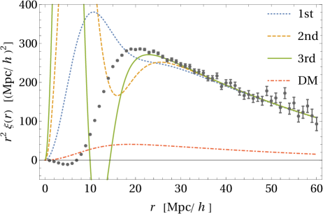
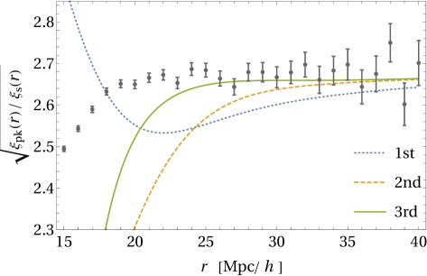
Figure 1: Correlation functions for matter and peaks of height $\nu_{\mathrm{c}}=2.5$ with a flat $\Lambda$CDM model. Left panel: Correlation functions of matter (blue) and of peaks with 1st-order (orange), 2nd-order (green), and 3rd-order (red) approximations. The points with error bars represent the results of numerical integrations of peak correlation function. Right panel: The scale-dependent bias of peaks with corresponding approximations.

In the following calculations, the power spectrum of the underlying density field is calculated by a Boltzmann code CLASS class11 ; CLASS with a flat $\Lambda$CDM model and cosmological parameters $h=0.6732$, $\Omega_{\mathrm{b}0}h^{2}=0.02238$, $\Omega_{\mathrm{cdm}}h^{2}=0.1201$, $n_{\mathrm{s}}=0.9660$, $\sigma_{8}=0.8120$ (Planck 2018 Planck2018 ). We apply a smoothing radius of $R=5\,h^{-1}\mathrm{Mpc}$ for the underlying mass density field, and apply a peak threshold of $\nu_{\mathrm{c}}=2.5$. Fig. 1 shows the correlation function of peaks given by Eq. (46), with approximations up to 1st, 2nd and 3rd orders. The correlation function of the underlying mass density field is also plotted. The points with error bars are the results of a 14-dimensional Monte-Carlo integration of the full expression of the peak correlation function as described in Sec. IV.1 .

In the left figure, the correlation functions are multiplied by $r^{2}$. The three approximations are almost identical on large scales $r\gtrsim 40\,h^{-1}\mathrm{Mpc}$, which means that the 1st-order approximation is already accurate enough to describe the correlation function on these scales. The three approximations then deviate from each other on smaller scales, $r\lesssim 40\,h^{-1}\mathrm{Mpc}$. A remarkable structure of the higher-order approximations is the decrease of the correlation function on small scales which is seen around $r\sim 20\,h^{-1}\mathrm{Mpc}$. This structure is explained by the exclusion effect of peaks BCDP16 ; CPP18 : the peaks cannot be too close to each other in the smoothed density field in particular because of the constraint on the sign of the curvatures. Hence, the correlation function of peaks should be negative around the scales of the smoothing radius. In the Monte-Carlo integration, this exclusion effect is accurately seen as expected. In the perturbative approximations, the exclusion effect is not sufficiently seen in the first-order approximation. In the third-order approximation, the correlation function actually becomes negative on small scales. However, higher-order contributions becomes more important on sufficiently small scales, and behaviors on small scales in our approximations do not correspond to the true correlation function of peaks, highlighting the rather poor convergence of the perturbative bias expansion on small scales which can not capture the non-perturbative exclusion zone.

However, the perturbative method and the Monte-Carlo approach are complementary. The small-scale behaviors, including the exclusion effect, are accurately captured by a Monte-Carlo method, while the large-scale behaviors are more accurately and efficiently evaluated by perturbative methods. The computational time of the perturbative method is of the order of a few seconds for this figure, while that of the Monte-Carlo method is of the order of a couple of days on 7 nodes with 64 cores each. The perturbative method is suited for evaluating large-scale correlations, while the Monte-Carlo method is better suited for evaluating small-scale correlations and exclusion effects.

To precisely see differences among approximations of various orders, the scale-dependent bias, $[\xi_{\mathrm{pk}}(r)/\xi_{\mathrm{s}}(r)]^{1/2}$, is plotted in the right-hand panel of Fig. 1, where $\xi_{\mathrm{s}}(r)=\xi^{(0)}_{0}(r)$ is the correlation function of the underlying mass density field. This figure shows percent-level differences among the different approximations. The differences between first-order and higher-order approximations are within a percent for $r\gtrsim 40\,h^{-1}\mathrm{Mpc}$. The difference between second-order and third-order approximations are within a percent for $r\gtrsim 30\,h^{-1}\mathrm{Mpc}$. Therefore, we can reliably apply second-order approximation in the last range of scales. Comparing with the results of Monte-Carlo integration, the third-order approximation looks accurate at the percent-level for $r\gtrsim 25\,h^{-1}\mathrm{Mpc}$.

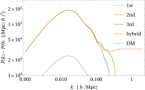
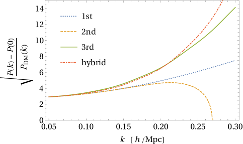
Figure 2: Power spectra in the linear density field with a flat $\Lambda$CDM model. The zero-lag value $P(k\rightarrow 0)$ is subtracted from each power spectrum. Left panel: Power spectra of matter (violet) and of peaks with 1st-order (blue), 2nd-order (orange), 3rd-order (green) approximations, and the “hybrid” data (red) are plotted. Right panel: The scale-dependent bias of the power spectra (with zero-lag values subtracted off) with corresponding approximations.

Next we consider the power spectrum of peaks by Fourier transforming the correlation function obtained above. The behavior of the correlation function below the scales of the exclusion zone ($\lesssim 20\,h^{-1}\mathrm{Mpc}$) non-trivially affects the power spectrum even on large scales ($k\rightarrow 0$), engendering a sub-Poissonian behavior of peaks that was already discussed in Refs. Bal13 ; BCDP16 in 1D. This effect of exclusion zone has highly non-perturbative nature and cannot be captured by the large-separation expansions. In this paper, we just remove the effect of exclusion zone by subtracting off the zero-lag value $P(k\rightarrow 0)$ from the power spectra, and the results are given in Fig. 2.

In this figure, we also plot the power spectrum from the “hybrid” correlation function, which is a composition of the interpolated MCMC results for $r<30\,h^{-1}\mathrm{Mpc}$ and 3rd-order approximation for $r>30\,h^{-1}\mathrm{Mpc}$. Neglecting the constant components from the effect of exclusion zone, the power spectrum of the large-separation expansion gives a good prediction for $k\lesssim 0.1$–$0.2\,h\mathrm{Mpc}^{-1}$. However, the large-separation expansions gives positive value of $P(k\rightarrow 0)$ while the hybrid data including the exclusion effects gives a negative value of the same quantity (which is why removing this negative constant to get the red dot-dashed line gives a positive plateau on small scales). A more detailed investigation of the effect of the exclusion zone in 3D is beyond the scope of this paper which focuses on large-separation expansions, and will be investigated thoroughly in a dedicated paper.

V Conclusions

In this paper, we revisit the problem of estimating peak clustering within a large-separation expansion. We derive a set of formulas to evaluate the correlation function of peaks in Gaussian random fields in general. The renormalized bias functions of peaks are derived from the definition up to third order, and the resultant correlation function of peaks are represented by an analytic form which can be evaluated with 1D FFT only. Thus the numerical evaluations of the formula is very fast.

The result of the derived formula are compared with a Monte-Carlo 14D integrations of the exact expression of the peak correlation function. The results are consistent with each other on large scales, where the large-separation expansion is sufficiently accurate ($r\gtrsim 25\,h^{-1}\mathrm{Mpc}$). On small scales, the Monte-Carlo method is able to provide an accurate estimate including the exclusion effect which is essentially non-perturbative and cannot be captured by our bias expansion. Therefore, both methods are quite complementary to each other.

In connection to the structure formation, the correlation of peaks in this paper are evaluated in Lagrangian space. Dynamical evolutions of the peak positions should be taken into account for the predictions in Eulerian space. The iPT Mat11 ; Mat12 ; Mat14 ; MD16 offers a systematic method to perturbatively evaluate the clustering in Eulerian space. Including the dynamical evolutions by iPT, the results of higher-order perturbation theory should also be reduced to expressions with 1D FFT, using the technique of Ref. SVM16 ; SV16 ; MFHB16 ; FBMH17 . Deriving the concrete expressions in Eulerian space using the iPT up to third order will be addressed in future work.

Appendix A A direct derivation of the renormalized bias functions of peaks

In this Appendix, the explicit form of renormalized bias functions of peaks up to third order, Eqs. (26)–(III.2), are derived from the original definition of the functions. The first and second order results are already given in Ref. MD16 . This Appendix is a straightforward generalization of the last work to the third order. In this paper, the window function $W(kR)$ is included in the power spectrum $P_{\mathrm{s}}(k)$ in Eq. (23), while it is included in the renormalized bias functions $c_{n}$ in Ref. MD16 .

The distribution function $P(\bm{y})$ is given by Eq. (II.1). The Fourier transform of the variables $y_{\alpha}(\bm{x})$ has a form,

$$\tilde{y}_{\alpha}(\bm{k})=U_{\alpha}(\bm{k})\tilde{\delta}_{\mathrm{s}}(\bm{k})$$ (52)

where the functions $U_{\alpha}(\bm{k})$ are given by

$$\left[U_{\alpha}(\bm{k})\right]=\left(\frac{1}{\sigma_{0}},\frac{ik_{1}}{\sigma_{1}},\frac{ik_{2}}{\sigma_{1}},\frac{ik_{3}}{\sigma_{1}},\frac{-{k_{1}}^{2}}{\sigma_{2}},\frac{-{k_{2}}^{2}}{\sigma_{2}},\frac{-{k_{3}}^{2}}{\sigma_{2}},\frac{-k_{1}k_{2}}{\sigma_{2}},\frac{-k_{2}k_{3}}{\sigma_{2}},\frac{-k_{1}k_{3}}{\sigma_{2}}\right).$$ (53)

We define a differential operator

$$\mathcal{D}(\bm{k})\equiv\sum_{\alpha}U_{\alpha}(\bm{k})\frac{\partial}{\partial y_{\alpha}}=\frac{1}{\sigma_{0}}\frac{\partial}{\partial\nu}+\frac{i}{\sigma_{1}}\bm{k}\cdot\frac{\partial}{\partial\bm{\eta}}-\frac{1}{\sigma_{2}}\sum_{i\leq j}k_{i}k_{j}\frac{\partial}{\partial\zeta_{ij}}.$$ (54)

With this operator, the renormalized bias functions of Eq. (25) are given by

$$c_{n}(\bm{k}_{1},\ldots,\bm{k}_{n})=\frac{1}{\bar{N}_{\mathrm{pk}}}\left\langle\mathcal{D}(\bm{k}_{1})\cdots\mathcal{D}(\bm{k}_{n})N_{\mathrm{pk}}\right\rangle=\frac{(-1)^{n}}{\bar{N}_{\mathrm{pk}}}\int d^{10}y\,N_{\mathrm{pk}}(\bm{y})\mathcal{D}(\bm{k}_{1})\cdots\mathcal{D}(\bm{k}_{n})\mathcal{P}(\bm{y}).$$ (55)

The first equality in the above equation can be derived by Fourier transforming Eq. (25) with respect to $\bm{k}$, and partial integrations are applied in the second equality.

Although independent set of variables $\zeta_{ij}$ are given for $i\leq j$, it is useful to introduce a set of symmetric tensor

$$\xi_{ij}\equiv\begin{cases}\zeta_{ij}&(i\leq j),\\ \zeta_{ji}&(i>j).\end{cases}$$ (56)

Any function of $\zeta_{ij}$ $(i\leq j)$ can be considered as a function of $\xi_{ij}$. The differentiation with respect to variables $\zeta_{ij}$ is given by

$$\frac{\partial}{\partial\zeta_{ij}}=\begin{cases}\frac{\partial}{\partial\xi_{ij}}&(i=j),\\ \frac{\partial}{\partial\xi_{ij}}+\frac{\partial}{\partial\xi_{ji}}&(i<j).\end{cases}$$ (57)

With these new variables, the differential operator $\mathcal{D}(\bm{k})$ of Eq. (54) reduces to

$$\mathcal{D}(\bm{k})\equiv\sum_{\alpha}U_{\alpha}(\bm{k})\frac{\partial}{\partial y_{\alpha}}=\frac{1}{\sigma_{0}}\frac{\partial}{\partial\nu}+\frac{i}{\sigma_{1}}k_{i}\frac{\partial}{\partial\eta_{i}}-\frac{1}{\sigma_{2}}k_{i}k_{j}\frac{\partial}{\partial\xi_{ij}},$$ (58)

where repeated indices $i,j$ are summed over. Rotationally invariant quantities $\eta^{2}$, $J_{1}$, $J_{2}$, $J_{3}$ are just given by Eqs. (10) and (11) with replacements $\zeta_{ij}\rightarrow\xi_{ij}$:

$$\eta^{2}\equiv\bm{\eta}\cdot\bm{\eta},\quad J_{1}\equiv-\xi_{ii},\quad J_{2}\equiv\frac{3}{2}\tilde{\xi}_{ij}\tilde{\xi}_{ji},\quad J_{3}\equiv\frac{9}{2}\tilde{\xi}_{ij}\tilde{\xi}_{jk}\tilde{\xi}_{ki},$$ (59)

with

$$\tilde{\xi}_{ij}\equiv\xi_{ij}+\frac{1}{3}\delta_{ij}J_{1}.$$ (60)

To calculate the differentiations of the last expression of Eq. (55), the relations

$$\frac{\partial(\eta^{2})}{\partial\eta_{i}}=2\eta_{i},\quad\frac{\partial J_{1}}{\partial\xi_{ij}}=-\delta_{ij},\quad\frac{\partial J_{2}}{\partial\xi_{ij}}=3\tilde{\xi}_{ji},\quad\frac{\partial\tilde{\xi}_{kl}}{\partial\xi_{ij}}=\delta_{ik}\delta_{jl}-\frac{1}{3}\delta_{ij}\delta_{kl}$$ (61)

are useful. The distribution function $P(\bm{y})$ depends only on four rotationally invariant variables $\nu$, $\eta^{2}$, $J_{1}$ and $J_{2}$ as given in Eq. (II.1). Using the above relations, the first-order derivatives are given by

$$\frac{\partial}{\partial\eta_{i}}\mathcal{P}=2\eta_{i}\frac{\partial}{\partial(\eta^{2})}\mathcal{P},\quad\frac{\partial}{\partial\xi_{ij}}\mathcal{P}=\left[-\delta_{ij}\frac{\partial}{\partial J_{1}}+3\tilde{\xi}_{ji}\frac{\partial}{\partial J_{2}}\right]\mathcal{P},$$ (62)

the second-order derivatives are given by

$$\frac{\partial^{2}}{\partial\eta_{i}\partial\eta_{j}}\mathcal{P} =2\left[\delta_{ij}\frac{\partial}{\partial(\eta^{2})}+2\eta_{i}\eta_{j}\frac{\partial^{2}}{\partial(\eta^{2})^{2}}\right]\mathcal{P},$$ (63)

$$\frac{\partial^{2}}{\partial\xi_{ij}\partial\xi_{kl}}\mathcal{P} =\left[\delta_{ij}\delta_{kl}\frac{\partial^{2}}{\partial{J_{1}}^{2}}-3\left(\delta_{ij}\tilde{\xi}_{lk}+\delta_{kl}\tilde{\xi}_{ji}\right)\frac{\partial^{2}}{\partial J_{1}\partial J_{2}}+9\tilde{\xi}_{ji}\tilde{\xi}_{lk}\frac{\partial^{2}}{\partial{J_{2}}^{2}}+\left(3\delta_{il}\delta_{jk}-\delta_{ij}\delta_{kl}\right)\frac{\partial}{\partial J_{2}}\right]\mathcal{P},$$ (64)

and the third-order derivatives are given by

$$\frac{\partial^{3}}{\partial\eta_{i}\partial\eta_{j}\partial\eta_{k}}\mathcal{P} =4\left[\left(\delta_{ij}\eta_{k}+\delta_{jk}\eta_{i}+\delta_{ki}\eta_{j}\right)\frac{\partial^{2}}{\partial(\eta^{2})^{2}}+2\eta_{i}\eta_{j}\eta_{k}\frac{\partial^{3}}{\partial(\eta^{2})^{3}}\right]\mathcal{P},$$ (65)

$$\frac{\partial^{3}}{\partial\xi_{ij}\partial\xi_{kl}\partial\xi_{mn}}\mathcal{P} =\left[-\delta_{ij}\delta_{kl}\delta_{mn}\frac{\partial^{3}}{\partial{J_{1}}^{3}}+3\left(\delta_{ij}\delta_{kl}\tilde{\xi}_{nm}+\delta_{ij}\delta_{mn}\tilde{\xi}_{lk}+\delta_{kl}\delta_{mn}\tilde{\xi}_{ji}\right)\frac{\partial^{3}}{\partial{J_{1}}^{2}\partial J_{2}}-9\left(\delta_{ij}\tilde{\xi}_{lk}\tilde{\xi}_{nm}+\delta_{kl}\tilde{\xi}_{ji}\tilde{\xi}_{nm}+\delta_{mn}\tilde{\xi}_{ji}\tilde{\xi}_{lk}\right)\frac{\partial^{3}}{\partial J_{1}\partial{J_{2}}^{2}}\right.$$

$$\quad+27\tilde{\xi}_{ji}\tilde{\xi}_{lk}\tilde{\xi}_{nm}\frac{\partial^{3}}{\partial{J_{2}}^{3}}+3\left(\delta_{ij}\delta_{kl}\delta_{mn}-\delta_{ij}\delta_{kn}\delta_{lm}-\delta_{kl}\delta_{in}\delta_{jm}-\delta_{il}\delta_{jk}\delta_{mn}\right)\frac{\partial^{2}}{\partial J_{1}\partial J_{2}}$$

$$\quad\left.+\,3\left(3\delta_{in}\delta_{jm}\tilde{\xi}_{lk}+3\delta_{kn}\delta_{lm}\tilde{\xi}_{ji}+3\delta_{il}\delta_{jk}\tilde{\xi}_{nm}-\delta_{ij}\delta_{kl}\tilde{\xi}_{nm}-\delta_{ij}\delta_{mn}\tilde{\xi}_{lk}-\delta_{kl}\delta_{mn}\tilde{\xi}_{ji}\right)\frac{\partial^{2}}{\partial{J_{2}}^{2}}\right]\mathcal{P}.$$ (66)

In calculating Eq. (55), one notices that the number density $N_{\mathrm{pk}}$ and the distribution function $\mathcal{P}(\bm{y})$ only depend on rotationally invariant variables. Thus we can first average over the angular dependence in the product of operators $\mathcal{D}(\bm{k})$, which appears only in the coefficients of Eqs. (62)–(A). Denoting the angular average by $\langle\cdots\rangle_{\Omega}$, we have

$$\left\langle\eta_{i}\right\rangle_{\Omega}=0,\quad\left\langle\eta_{i}\eta_{j}\right\rangle_{\Omega}=\frac{1}{3}\delta_{ij}\eta^{2},\quad\left\langle\tilde{\xi}_{ij}\right\rangle_{\Omega}=0,\quad\left\langle\tilde{\xi}_{ij}\tilde{\xi}_{kl}\right\rangle_{\Omega}=\frac{1}{15}\left(\delta_{ik}\delta_{jl}+\delta_{il}\delta_{jk}-\frac{2}{3}\delta_{ij}\delta_{kl}\right)J_{2},$$ (67)

$$\left\langle\tilde{\xi}_{ij}\tilde{\xi}_{kl}\tilde{\xi}_{mn}\right\rangle_{\Omega}=\frac{1}{315}\left[\frac{16}{3}\delta_{ij}\delta_{kl}\delta_{mn}-4\left(\delta_{ij}\delta_{km}\delta_{ln}+\delta_{ij}\delta_{kn}\delta_{lm}+\delta_{kl}\delta_{im}\delta_{jn}+\delta_{kl}\delta_{in}\delta_{jm}+\delta_{mn}\delta_{ik}\delta_{jl}+\delta_{mn}\delta_{il}\delta_{jk}\right)\right.$$

$$\hskip 84.0pt\left.+\,3\left(\delta_{ik}\delta_{lm}\delta_{jn}+\delta_{jk}\delta_{lm}\delta_{in}+\delta_{il}\delta_{km}\delta_{jn}+\delta_{ik}\delta_{ln}\delta_{jm}+\delta_{jl}\delta_{km}\delta_{in}+\delta_{il}\delta_{kn}\delta_{jm}+\delta_{jk}\delta_{ln}\delta_{im}+\delta_{jl}\delta_{kn}\delta_{im}\right)\right]J_{3}.$$ (68)

The angular averages can be taken for the operators in the integrand of Eq. (55):

$$c_{n}(\bm{k}_{1},\ldots,\bm{k}_{n})=\frac{(-1)^{n}}{\bar{N}_{\mathrm{pk}}}\int d^{10}y\,N_{\mathrm{pk}}(\bm{y})\langle\mathcal{D}(\bm{k}_{1})\cdots\mathcal{D}(\bm{k}_{n})\rangle_{\Omega}\mathcal{P}(\bm{y}).$$ (69)

Using the above equations, the results up to third order are given by

$$\left\langle\mathcal{D}(\bm{k})\right\rangle_{\Omega}\mathcal{P} =\left(\frac{1}{\sigma_{0}}\frac{\partial}{\partial\nu}+\frac{k^{2}}{\sigma_{2}}\frac{\partial}{\partial J_{1}}\right)\mathcal{P},$$ (70)

$$\left\langle\mathcal{D}(\bm{k}_{1})\mathcal{D}(\bm{k}_{2})\right\rangle_{\Omega}\mathcal{P} =\left\{\left(\frac{1}{\sigma_{0}}\frac{\partial}{\partial\nu}+\frac{{k_{1}}^{2}}{\sigma_{2}}\frac{\partial}{\partial J_{1}}\right)\left(\frac{1}{\sigma_{0}}\frac{\partial}{\partial\nu}+\frac{{k_{2}}^{2}}{\sigma_{2}}\frac{\partial}{\partial J_{1}}\right)\right.$$

$$\qquad\left.-\frac{2(\bm{k}_{1}\cdot\bm{k}_{2})}{{\sigma_{1}}^{2}}\left[1+\frac{2}{3}\eta^{2}\frac{\partial}{\partial(\eta^{2})}\right]\frac{\partial}{\partial(\eta^{2})}+\frac{3(\bm{k}_{1}\cdot\bm{k}_{2})^{2}-{k_{1}}^{2}{k_{2}}^{2}}{{\sigma_{2}}^{2}}\left[1+\frac{2}{5}{J_{2}}^{2}\frac{\partial}{\partial J_{2}}\right]\frac{\partial}{\partial J_{2}}\right\}\mathcal{P},$$ (71)

$$\left\langle\mathcal{D}(\bm{k}_{1})\mathcal{D}(\bm{k}_{2})\mathcal{D}(\bm{k}_{3})\right\rangle_{\Omega}\mathcal{P} =\left\{\left(\frac{1}{\sigma_{0}}\frac{\partial}{\partial\nu}+\frac{{k_{1}}^{2}}{\sigma_{2}}\frac{\partial}{\partial J_{1}}\right)\left(\frac{1}{\sigma_{0}}\frac{\partial}{\partial\nu}+\frac{{k_{2}}^{2}}{\sigma_{2}}\frac{\partial}{\partial J_{1}}\right)\left(\frac{1}{\sigma_{0}}\frac{\partial}{\partial\nu}+\frac{{k_{3}}^{2}}{\sigma_{2}}\frac{\partial}{\partial J_{1}}\right)\right.$$

$$\qquad-\frac{2(\bm{k}_{1}\cdot\bm{k}_{2})}{{\sigma_{1}}^{2}}\left(\frac{1}{\sigma_{0}}\frac{\partial}{\partial\nu}+\frac{{k_{3}}^{2}}{\sigma_{2}}\frac{\partial}{\partial J_{1}}\right)\left[1+\frac{2}{3}\eta^{2}\frac{\partial}{\partial(\eta^{2})}\right]\frac{\partial}{\partial(\eta^{2})}+\mathrm{cyc.}$$

$$\qquad+\frac{3(\bm{k}_{1}\cdot\bm{k}_{2})^{2}-{k_{1}}^{2}{k_{2}}^{2}}{{\sigma_{2}}^{2}}\left(\frac{1}{\sigma_{0}}\frac{\partial}{\partial\nu}+\frac{{k_{3}}^{2}}{\sigma_{2}}\frac{\partial}{\partial J_{1}}\right)\left[1+\frac{2}{5}{J_{2}}^{2}\frac{\partial}{\partial J_{2}}\right]\frac{\partial}{\partial J_{2}}+\mathrm{cyc.}$$

$$\qquad\left.+\frac{72}{35}\left[(\bm{k}_{1}\cdot\bm{k}_{2})(\bm{k}_{2}\cdot\bm{k}_{3})(\bm{k}_{3}\cdot\bm{k}_{1})-\frac{1}{3}{k_{1}}^{2}(\bm{k}_{2}\cdot\bm{k}_{3})+\mathrm{cyc.}+\frac{2}{9}{k_{1}}^{2}{k_{2}}^{2}{k_{3}}^{2}\right]J_{3}\frac{\partial^{3}}{{\partial J_{2}}^{3}}\right\}\mathcal{P}.$$ (72)

Substituting identities

$$\left[1+\frac{2}{3}\eta^{2}\frac{\partial}{\partial(\eta^{2})}\right]\frac{\partial}{\partial(\eta^{2})}e^{-3\eta^{2}/2} =-L^{(1/2)}_{1}\left(\frac{3}{2}\eta^{2}\right)e^{-3\eta^{2}/2},$$ (73)

$$\left[1+\frac{2}{5}J_{2}\frac{\partial}{\partial J_{2}}\right]\frac{\partial}{\partial J_{2}}e^{-5J_{2}/2} =-L^{(3/2)}_{1}\left(\frac{5}{2}J_{2}\right)e^{-5J_{2}/2},$$ (74)

$$J_{3}\frac{\partial^{3}}{{\partial J_{2}}^{3}}e^{-5J_{2}/2} =\frac{75\sqrt{7}}{8}F_{01}(5J_{2},J_{3})e^{-5J_{2}/2}$$ (75)

into Eqs. (70)–(A) and (69), the final results for the renormalized bias functions, Eqs. (26)–(III.2) are obtained.

Appendix B Orthogonal polynomials

In this Appendix, we give the definitions of the orthogonal polynomials of field variables to define the bias coefficients $c_{ijqlm}$ in Eq. (30). We closely follow the notation of Refs. GPP12 ; LMD16 ; Diz16 in this paper.

The first polynomials are the multivariate Hermite polynomials,

$$H_{ij}(\nu,J_{1})=\frac{1}{\mathcal{N}(\nu,J_{1})}\left(-\frac{\partial}{\partial\nu}\right)^{i}\left(-\frac{\partial}{\partial J_{1}}\right)^{j}\mathcal{N}(\nu,J_{1}),$$ (76)

where $\mathcal{N}(\nu,J_{1})$ is the joint distribution function of $\nu$ and $J_{1}$ which is given by Eq. (14). The multivariate Hermite polynomials satisfy the orthonormality condition,

$$\int_{-\infty}^{\infty}d\nu\,dJ_{1}\,\mathcal{N}(\nu,J_{1})\,H_{ij}(\nu,J_{1})\,H_{kl}(\nu,J_{1})=i!\,j!\,\delta_{ik}\delta_{jl}.$$ (77)

The second polynomials are the generalized Laguerre polynomials,

$$L^{(\alpha)}_{q}(x)=\frac{x^{-\alpha}e^{x}}{q!}\frac{d^{q}}{dx^{q}}\left(x^{q+\alpha}e^{-x}\right).$$ (78)

The Laguerre polynomials also satisfy an orthonormality condition,

$$\int_{0}^{\infty}dx\,e^{-x}x^{\alpha}L^{(\alpha)}_{n}(x)L^{(\alpha)}_{m}(x)=\frac{\Gamma(n+\alpha+1)}{n!}\delta_{nm}.$$ (79)

From this equation, we have

$$\int_{0}^{\infty}d(3\eta^{2})\,\chi_{3}^{2}(3\eta^{2})L^{(\alpha)}_{q}\left(\frac{3}{2}\eta^{2}\right)L^{(\alpha)}_{r}\left(\frac{3}{2}\eta^{2}\right)=\frac{\Gamma(q+3/2)}{q!\,\Gamma(3/2)}\delta_{qr},$$ (80)

where

$$\chi_{k}^{2}(x)\equiv\frac{x^{k/2-1}e^{-x/2}}{2^{k/2}\Gamma(k/2)}$$ (81)

is a chi-square distribution with $k$ degrees of freedom, and $\chi_{3}^{2}(3\eta^{2})$ corresponds to the distribution function of the variable $3\eta^{2}$.

The third polynomials are defined by,

$$F_{lm}(5J_{2},J_{3})=(-1)^{l}\sqrt{\frac{\Gamma(l+5/2)}{\Gamma\left(l+3m+5/2\right)}}\,\left(\frac{5}{2}J_{2}\right)^{3m/2}L^{(3m+3/2)}_{l}\left(\frac{5}{2}J_{2}\right)\,\mathsf{P}_{m}\left(\frac{J_{3}}{{J_{2}}^{3/2}}\right),$$ (82)

where

$$\mathsf{P}_{m}(x)=\frac{1}{2^{m}m!}\frac{d^{m}}{dx^{m}}(x^{2}-1)^{m}$$ (83)

are the Legendre polynomials, and satisfy the orthonormality condition,

$$\int_{-1}^{1}dx\,e^{-x}\mathsf{P}_{n}(x)\,\mathsf{P}_{m}(x)=\frac{2}{2n+1}\delta_{nm}.$$ (84)

The polynomials $F_{lm}$ satisfy orthonormality relations

$$\int_{0}^{\infty}d(5J_{2})\int_{-{J_{2}}^{3/2}}^{{J_{2}}^{3/2}}dJ_{3}\,p(5J_{2},J_{3})\,F_{lm}(5J_{2},J_{3})\,F_{l^{\prime}m^{\prime}}(5J_{2},J_{3})=\frac{\Gamma(l+5/2)}{\Gamma(5/2)\,l!\,(2m+1)}\delta_{ll^{\prime}}\delta_{mm^{\prime}},$$ (85)

where

$$p(5J_{2},J_{3})=\frac{\chi^{2}_{5}(5J_{2})}{2{J_{2}}^{3/2}}\Theta\left(1-{J_{3}}^{2}/{J_{2}}^{3}\right)=\frac{5^{3/2}}{6\sqrt{2\pi}}e^{-5J_{2}/2}\Theta\left(1-{J_{3}}^{2}/{J_{2}}^{3}\right)$$ (86)

is the joint probability distribution function of the variables $5J_{2}$ and $J_{3}$. The above orthonormality relations and Eq. (30) show that the bias coefficients $c_{ijqlm}$ is the expansion coefficients of $N_{\mathrm{pk}}$ by orthogonal polynomials,

$$N_{\mathrm{pk}}(\nu_{\mathrm{c}},\bm{x})=\bar{N}_{\mathrm{pk}}(\nu_{\mathrm{c}})\sum_{i,j,q,l,m}\frac{(-1)^{q}\,q!\,l!\,\Gamma(3/2)\,\Gamma(5/2)\,(2m+1)}{i!\,j!\,\Gamma(q+3/2)\,\Gamma(l+5/2)}{\sigma_{0}}^{i}\,{\sigma_{1}}^{2q}\,{\sigma_{2}}^{j+2l+3m}\,c_{ijqlm}(\nu_{\mathrm{c}})\,H_{ij}(\nu,J_{1})\,L^{(1/2)}_{q}\left(3\eta^{2}/2\right)\,F_{lm}\left(5J_{2},J_{3}\right).$$ (87)

See Refs. GPP12 ; LMD16 for the original motivation behind the introduction of these polynomials.

Appendix C Proof of Eq. (33)

In this Appendix, we derive the formula of Eq. (33) from the original definition of Eq. (30). The calculation is quite similar to those of Ref. BBKS .

Taking into account the property of Eq. (31), the definition of the bias coefficients, Eq. (30), reduces to

$$c_{ijqlm}(\nu_{\mathrm{c}})=\frac{\chi_{q}}{{\sigma_{0}}^{i}\,{\sigma_{2}}^{j+2l+3m}}\frac{\int d^{10}y\,\mathcal{P}(\bm{y})\,N_{\mathrm{pk}}(\nu_{\mathrm{c}})\,H_{ij}(\nu,J_{1})\,F_{lm}\left(5J_{2},J_{3}\right)}{\int d^{10}y\,\mathcal{P}(\bm{y})\,N_{\mathrm{pk}}(\nu_{\mathrm{c}})}.$$ (88)

Because the integrands in the rhs are rotationally invariant, the angular degrees of freedom do not contribute to the integrals. We define invariant variables,

$$x\equiv\lambda_{1}+\lambda_{2}+\lambda_{3},\quad y\equiv\frac{1}{2}(\lambda_{1}-\lambda_{3}),\quad z\equiv\frac{1}{2}(\lambda_{1}-2\lambda_{2}+\lambda_{3}),$$ (89)

where $\lambda_{1},\lambda_{2},\lambda_{3}$ are eigenvalues of $-\,\zeta_{ij}$ with a descending order ($\lambda_{1}\geq\lambda_{2}\geq\lambda_{3}$). With these variables, we have

$$J_{1}=x,\quad J_{2}=3y^{2}+z^{2},\quad J_{3}=z^{3}-9y^{2}z.$$ (90)

The peak number density of Eq. (II.2) reduces to

$$N_{\mathrm{pk}}(\nu_{\mathrm{c}})=\frac{2}{\sqrt{3}{R_{*}}^{3}}\Xi(\nu,\nu_{\mathrm{c}})\,\delta_{\mathrm{D}}^{3}(\bm{\eta})\,(x-2z)\left[(x+z)^{2}-(3y)^{2}\right]\Theta(y-z)\Theta(y+z)\Theta(x-3y+z).$$ (91)

The probability distribution function of the variables $\nu,x,y,z$ are given by BBKS

$$\mathcal{P}(\bm{y})d^{10}y\propto\mathcal{N}(\nu,x)\left|y\left(y^{2}-z^{2}\right)\right|e^{-5(3y^{2}+z^{2})/2}\,d\nu\,dx\,dy\,dz,$$ (92)

besides distributions of $\bm{\eta}$ and angular degrees of freedom. Multiplying Eqs. (91) and (92), and substituting the resulting expression into Eq. (88), the Eq. (33) is proven.

Appendix D Analytic expression of perturbed correlation function of peaks

In this Appendix, the functions $\xi_{\mathrm{pk}}^{(N)}(r)$ in Eq. (46) for $N=1,2,3$ are explicitly given in terms of the generalized correlation function, $\xi^{(n)}_{l}(r)$. The derivation is straightforward: Eqs. (26)–(III.2) are squared and substituted into Eq. (23), and formulas of Eqs. (39) and (42) are applied. The result of $N=3$ is derived by a use of the software package, Mathematica.

For $N=1$, we have

$$\xi_{\mathrm{pk}}^{(1)}(r)={b_{10}}^{2}\xi^{(0)}_{0}(r)+2b_{10}b_{01}\xi^{(2)}_{0}(r)+{b_{01}}^{2}\xi^{(4)}_{0}(r).$$ (93)

For $N=2$, we have

$$\xi_{\mathrm{pk}}^{(2)} ={b_{20}}^{2}\left(\xi^{(0)}_{0}\right)^{2}+4b_{20}b_{11}\xi^{(0)}_{0}\xi^{(2)}_{0}+2{b_{11}}^{2}\xi^{(0)}_{0}\xi^{(4)}_{0}+2\left(b_{20}b_{02}+{b_{11}}^{2}+\frac{2}{3}{\chi_{1}}^{2}\right)\left(\xi^{(2)}_{0}\right)^{2}+4b_{11}b_{02}\xi^{(2)}_{0}\xi^{(4)}_{0}+4b_{20}\chi_{1}\left(\xi^{(1)}_{1}\right)^{2}$$

$$\quad+8b_{11}\chi_{1}\xi^{(1)}_{1}\xi^{(3)}_{1}+\left({b_{02}}^{2}+\frac{4}{5}{\omega_{10}}^{2}\right)\left(\xi^{(4)}_{0}\right)^{2}+4\left(b_{02}+\frac{4}{5}\omega_{10}\right)\chi_{1}\left(\xi^{(3)}_{1}\right)^{2}+4\left(b_{20}\omega_{10}+\frac{2}{3}{\chi_{1}}^{2}\right)\left(\xi^{(2)}_{2}\right)^{2}+8b_{11}\omega_{10}\xi^{(2)}_{2}\xi^{(4)}_{2}$$

$$\quad+4\left(b_{02}+\frac{2}{7}\omega_{10}\right)\omega_{10}\left(\xi^{(4)}_{2}\right)^{2}+\frac{24}{5}\chi_{1}\omega_{10}\left(\xi^{(3)}_{3}\right)^{2}+\frac{72}{35}{\omega_{10}}^{2}\left(\xi^{(4)}_{4}\right)^{2}.$$ (94)

Finally, for $N=3$, we have

$$\xi_{\mathrm{pk}}^{(3)} ={b_{30}}^{2}\left(\xi^{(0)}_{0}\right)^{3}+6{b_{21}}{b_{30}}\xi^{(2)}_{0}\left(\xi^{(0)}_{0}\right)^{2}+3{b_{21}}^{2}\xi^{(4)}_{0}\left(\xi^{(0)}_{0}\right)^{2}+12{b_{10}}{b_{30}}{\chi_{1}}\left(\xi^{(1)}_{1}\right)^{2}\xi^{(0)}_{0}+2\left(3{b_{21}}^{2}+2{b_{10}}^{2}{\chi_{1}}^{2}+3{b_{12}}{b_{30}}\right)\left(\xi^{(2)}_{0}\right)^{2}\xi^{(0)}_{0}$$

$$\quad+4\left(2{b_{10}}^{2}{\chi_{1}}^{2}+3{b_{30}}{c_{10010}}\right)\left(\xi^{(2)}_{2}\right)^{2}\xi^{(0)}_{0}+12{\chi_{1}}\left({b_{10}}{b_{12}}+\frac{4}{5}{b_{10}}{c_{10010}}\right)\left(\xi^{(3)}_{1}\right)^{2}\xi^{(0)}_{0}+\frac{72}{5}{b_{10}}{\chi_{1}}{c_{10010}}\left(\xi^{(3)}_{3}\right)^{2}\xi^{(0)}_{0}$$

$$\quad+3\left({b_{12}}^{2}+\frac{4}{5}{c_{10010}}^{2}\right)\left(\xi^{(4)}_{0}\right)^{2}\xi^{(0)}_{0}+12\left(\frac{2}{7}{c_{10010}}+{b_{12}}\right){c_{10010}}\left(\xi^{(4)}_{2}\right)^{2}\xi^{(0)}_{0}+\frac{216}{35}{c_{10010}}^{2}\left(\xi^{(4)}_{4}\right)^{2}\xi^{(0)}_{0}+24{b_{10}}{b_{21}}{\chi_{1}}\xi^{(1)}_{1}\xi^{(3)}_{1}\xi^{(0)}_{0}$$

$$\quad+12{b_{12}}{b_{21}}\xi^{(2)}_{0}\xi^{(4)}_{0}\xi^{(0)}_{0}+24{b_{21}}{c_{10010}}\xi^{(2)}_{2}\xi^{(4)}_{2}\xi^{(0)}_{0}+2\left(4{b_{01}}{b_{10}}{\chi_{1}}^{2}+3{b_{12}}{b_{21}}+{b_{03}}{b_{30}}\right)\left(\xi^{(2)}_{0}\right)^{3}+\frac{4}{3}{b_{30}}{\varpi_{01}}\left(\xi^{(2)}_{2}\right)^{3}$$

$$\quad+\left({b_{03}}^{2}+\frac{12}{5}{c_{01010}}^{2}+\frac{14}{225}{\varpi_{01}}^{2}\right)\left(\xi^{(4)}_{0}\right)^{3}-4\left(\frac{12}{7}{c_{01010}}^{2}+\frac{41}{3087}{\varpi_{01}}^{2}-\frac{1}{3}{b_{03}}{\varpi_{01}}+\frac{6}{49}{c_{01010}}{\varpi_{01}}\right)\left(\xi^{(4)}_{2}\right)^{3}$$

$$\quad+\frac{1296}{8575}{\varpi_{01}}^{2}\left(\xi^{(4)}_{4}\right)^{3}+4\left(4{b_{01}}{b_{10}}{\chi_{1}}^{2}+3{b_{30}}{c_{01010}}+3{b_{21}}{c_{10010}}\right)\xi^{(2)}_{0}\left(\xi^{(2)}_{2}\right)^{2}+4{\chi_{1}}\left(3{b_{03}}{b_{10}}+3{b_{01}}{b_{12}}-2{b_{01}}^{2}{\chi_{1}}\right)\xi^{(2)}_{0}\left(\xi^{(3)}_{1}\right)^{2}$$

$$\quad+\frac{48}{5}{\chi_{1}}\left({b_{10}}{c_{01010}}+{b_{01}}{c_{10010}}\right)\xi^{(2)}_{0}\left(\xi^{(3)}_{1}\right)^{2}+8{\chi_{1}}\left(2{b_{01}}^{2}{\chi_{1}}-\frac{12}{5}{b_{10}}{c_{01010}}+\frac{7}{25}{b_{10}}{\varpi_{01}}\right)\xi^{(2)}_{2}\left(\xi^{(3)}_{1}\right)^{2}$$

$$\quad+\frac{72}{5}{\chi_{1}}\left({b_{10}}{c_{01010}}+{b_{01}}{c_{10010}}\right)\xi^{(2)}_{0}\left(\xi^{(3)}_{3}\right)^{2}+\frac{96}{25}{b_{10}}{\chi_{1}}{\varpi_{01}}\xi^{(2)}_{2}\left(\xi^{(3)}_{3}\right)^{2}+6\left({b_{03}}{b_{12}}+\frac{4}{5}{c_{01010}}{c_{10010}}\right)\xi^{(2)}_{0}\left(\xi^{(4)}_{0}\right)^{2}$$

$$\quad+12\left({b_{12}}{c_{01010}}+{b_{03}}{c_{10010}}+\frac{4}{7}{c_{01010}}{c_{10010}}\right)\xi^{(2)}_{0}\left(\xi^{(4)}_{2}\right)^{2}+4\left({b_{12}}{\varpi_{01}}-\frac{24}{7}{c_{01010}}{c_{10010}}-\frac{6}{49}{c_{10010}}{\varpi_{01}}\right)\xi^{(2)}_{2}\left(\xi^{(4)}_{2}\right)^{2}$$

$$\quad+2\left(6{b_{03}}{c_{01010}}+\frac{144}{35}{c_{01010}}^{2}-\frac{1}{35}{\varpi_{01}}^{2}-\frac{8}{5}{c_{01010}}{\varpi_{01}}\right)\xi^{(4)}_{0}\left(\xi^{(4)}_{2}\right)^{2}+\frac{432}{35}{c_{01010}}{c_{10010}}\xi^{(2)}_{0}\left(\xi^{(4)}_{4}\right)^{2}+\frac{144}{49}{c_{10010}}{\varpi_{01}}\xi^{(2)}_{2}\left(\xi^{(4)}_{4}\right)^{2}$$

$$\quad+\frac{8}{35}\left({27}{c_{01010}}^{2}+\frac{3}{5}{\varpi_{01}}^{2}\right)\xi^{(4)}_{0}\left(\xi^{(4)}_{4}\right)^{2}+\frac{48}{49}{\varpi_{01}}\left(\frac{1}{7}{\varpi_{01}}+3{c_{01010}}\right)\xi^{(4)}_{2}\left(\xi^{(4)}_{4}\right)^{2}$$

$$\quad+4{\chi_{1}}\left(3{b_{10}}{b_{21}}+4{b_{01}}{b_{30}}-2{b_{10}}^{2}{\chi_{1}}\right)\left(\xi^{(1)}_{1}\right)^{2}\xi^{(2)}_{0}+16{b_{10}}^{2}{\chi_{1}}^{2}\left(\xi^{(1)}_{1}\right)^{2}\xi^{(2)}_{2}+8\chi_{1}\left(3{b_{10}}{b_{12}}+3{b_{01}}{b_{21}}-2{b_{01}}{b_{10}}{\chi_{1}}\right)\xi^{(1)}_{1}\xi^{(2)}_{0}\xi^{(3)}_{1}$$

$$\quad+32\chi_{1}\left({b_{01}}{b_{10}}{\chi_{1}}-\frac{3}{5}{b_{10}}{c_{10010}}\right)\xi^{(1)}_{1}\xi^{(2)}_{2}\xi^{(3)}_{1}+\frac{144}{5}{b_{10}}{\chi_{1}}{c_{10010}}\xi^{(1)}_{1}\xi^{(2)}_{2}\xi^{(3)}_{3}+\frac{144}{5}{b_{10}}{\chi_{1}}{c_{01010}}\xi^{(2)}_{2}\xi^{(3)}_{1}\xi^{(3)}_{3}$$

$$\quad-\frac{48}{25}{b_{10}}{\chi_{1}}{\varpi_{01}}\xi^{(2)}_{2}\xi^{(3)}_{1}\xi^{(3)}_{3}+12{b_{01}}{\chi_{1}}{b_{21}}\left(\xi^{(1)}_{1}\right)^{2}\xi^{(4)}_{0}+2\left(3{b_{12}}^{2}+2{b_{01}}^{2}{\chi_{1}}^{2}+3{b_{03}}{b_{21}}\right)\left(\xi^{(2)}_{0}\right)^{2}\xi^{(4)}_{0}$$

$$\quad+4\left(\frac{6}{5}{c_{10010}}^{2}+2{b_{01}}^{2}{\chi_{1}}^{2}+3{b_{21}}{c_{01010}}\right)\left(\xi^{(2)}_{2}\right)^{2}\xi^{(4)}_{0}+12b_{01}\chi_{1}\left({b_{03}}+\frac{4}{5}{c_{01010}}\right)\left(\xi^{(3)}_{1}\right)^{2}\xi^{(4)}_{0}+\frac{72}{5}{b_{01}}{\chi_{1}}{c_{01010}}\left(\xi^{(3)}_{3}\right)^{2}\xi^{(4)}_{0}$$

$$\quad+24{b_{01}}{b_{12}}{\chi_{1}}\xi^{(1)}_{1}\xi^{(3)}_{1}\xi^{(4)}_{0}+4\left({b_{21}}{\varpi_{01}}-\frac{12}{7}{c_{10010}}^{2}\right)\left(\xi^{(2)}_{2}\right)^{2}\xi^{(4)}_{2}+\frac{8}{5}b_{01}\chi_{1}\left(\frac{7}{5}{\varpi_{01}}-12{c_{01010}}\right)\left(\xi^{(3)}_{1}\right)^{2}\xi^{(4)}_{2}$$

$$\quad+\frac{96}{25}{b_{01}}{\chi_{1}}{\varpi_{01}}\left(\xi^{(3)}_{3}\right)^{2}\xi^{(4)}_{2}+24\left({b_{21}}{c_{01010}}+{b_{12}}{c_{10010}}\right)\xi^{(2)}_{0}\xi^{(2)}_{2}\xi^{(4)}_{2}-\frac{96}{5}{b_{01}}{\chi_{1}}{c_{10010}}\xi^{(1)}_{1}\xi^{(3)}_{1}\xi^{(4)}_{2}+\frac{144}{5}{b_{01}}{\chi_{1}}{c_{10010}}\xi^{(1)}_{1}\xi^{(3)}_{3}\xi^{(4)}_{2}$$

$$\quad+\frac{48}{5}b_{01}\chi_{1}\left(3{c_{01010}}-\frac{1}{5}{\varpi_{01}}\right)\xi^{(3)}_{1}\xi^{(3)}_{3}\xi^{(4)}_{2}+8\left(3{b_{12}}{c_{01010}}+\frac{6}{5}{c_{01010}}{c_{10010}}-\frac{2}{5}{c_{10010}}{\varpi_{01}}\right)\xi^{(2)}_{2}\xi^{(4)}_{0}\xi^{(4)}_{2}+\frac{432}{35}{c_{10010}}^{2}\left(\xi^{(2)}_{2}\right)^{2}\xi^{(4)}_{4}$$

$$\quad+\frac{24}{35}\left(18{c_{01010}}^{2}+\frac{17}{49}{\varpi_{01}}^{2}-\frac{24}{7}{c_{01010}}{\varpi_{01}}\right)\left(\xi^{(4)}_{2}\right)^{2}\xi^{(4)}_{4}+\frac{288}{35}{c_{10010}}\left(3{c_{01010}}-\frac{2}{7}{\varpi_{01}}\right)\xi^{(2)}_{2}\xi^{(4)}_{2}\xi^{(4)}_{4}.$$ (95)

Appendix E Contributions of local-type non-Gaussianity to the peak clustering

In this Appendix, we outline an example of evaluating the non-Gaussian contribution of Eq. (47) to the peak clustering. The local-type non-Gaussianity is considered to illustrate the calculation of this term. In the local-type non-Gaussianity, the bispectrum $B_{\zeta}(k_{1},k_{2},k_{3})$ of initial curvature perturbations $\zeta$ is given by

$$B_{\zeta}(k_{1},k_{2},k_{3})=\frac{6}{5}f_{\mathrm{NL}}\left[P_{\zeta}(k_{1})P_{\zeta}(k_{2})+\mathrm{cyc.}\right],$$ (96)

where $P_{\zeta}(k)$ is the power spectrum of $\zeta$. In Fourier space, $\tilde{\delta}(\bm{k})$ and $\tilde{\zeta}(\bm{k})$ are related by

$$\tilde{\delta}(\bm{k},t)=\mathcal{M}(k,t)\tilde{\zeta}(\bm{k},t),$$ (97)

where

$$\mathcal{M}(k,t)=\frac{2(1+w)}{5+3w}\frac{k^{2}T(k,t)}{a^{2}H^{2}\Omega}g(t).$$ (98)

In the above equation, $w=1/3$ in the radiation dominated (RD) era and $w=0$ in the matter dominated (MD) and the post MD eras. $T(k,t)$ is the transfer function which is non-unity on sub-horizon scales. The function $g(t)$ is the suppression factor of the potential in the post-MD epoch, i.e., $g(t)=D_{+}(t)/a(t)$ with a normalization of growth factor $D_{+}(t)\rightarrow a(t)$ in MD epoch. In the RD, MD, and after the MD epochs, we have

$$\mathcal{M}(k,t)=\begin{cases}\displaystyle\frac{4}{9}\left(\frac{k}{aH}\right)^{2}T_{\mathrm{r}}(k,t),&\mathrm{(RD)},\\ \displaystyle\frac{2}{5}\left(\frac{k}{aH}\right)^{2}T_{\mathrm{m}}(k,t),&\mathrm{(MD)},\\ \displaystyle\frac{2}{5}D_{+}(t)\frac{k^{2}T_{\mathrm{m}}(k,t)}{{H_{0}}^{2}\Omega_{\mathrm{m0}}},&\mathrm{(post\ MD)},\end{cases}$$ (99)

where $T_{\mathrm{r}}(k,t)=3^{3/2}(aH/k)j_{1}(k/(\sqrt{3}aH))$ is the transfer function in RD epoch, and $T_{\mathrm{m}}(k,t)$ is the transfer function in MD and post-MD epochs. We omit the time-dependence from the argument of functions and denote $\mathcal{M}(k)$, $T(k)$, etc. in the following, although all these functions depends on time, as well as the power spectrum $P(k)$ and the bispectrum $B(k_{1},k_{2},k_{3})$ etc.

From Eqs. (96), (97), the bispectrum of the smoothed density field $B_{\mathrm{s}}(k_{1},k_{2},k_{3})$ is given by

$$B_{\mathrm{s}}(k_{1},k_{2},k_{3})=\frac{6}{5}f_{\mathrm{NL}}\left[\frac{\mathcal{M}_{\mathrm{s}}(k_{3})P_{\mathrm{s}}(k_{1})P_{\mathrm{s}}(k_{2})}{\mathcal{M}_{\mathrm{s}}(k_{1})\mathcal{M}_{\mathrm{s}}(k_{2})}+\mathrm{cyc.}\right],$$ (100)

where $\mathcal{M}_{\mathrm{s}}(k)\equiv\mathcal{M}(k)W(kR)$. Substituting Eqs. (26), (III.2) and (100) into Eq. (47), we have an analytic expression of the $P^{\mathrm{NG}}_{\mathrm{pk}}(k)$. The same technique of subsection III.3 can also be applied, and the resulting expression reduces to the form which can be calculated very fast by using FFTLog. The result is given by

$$P^{\mathrm{NG}}_{\mathrm{pk}}(k) =c_{1}(k)\int_{\bm{k}_{12}=\bm{k}}c_{2}(\bm{k}_{1},\bm{k}_{2})B_{\mathrm{s}}(k,k_{1},k_{2})$$

$$=\frac{6}{5}f_{\mathrm{NL}}c_{1}(k)\Biggl{\{}\mathcal{M}_{\mathrm{s}}(k)\int_{0}^{\infty}4\pi r^{2}dr\,j_{0}(kr)\left[b_{20}\left(A^{(0)}_{0}\right)^{2}+2b_{11}A^{(0)}_{0}A^{(2)}_{0}+b_{02}\left(A^{(2)}_{0}\right)^{2}+2\chi_{1}\left(A^{(1)}_{1}\right)^{2}+2\omega_{10}\left(A^{(2)}_{2}\right)^{2}\right]$$

$$\hskip 60.0pt+\frac{2P_{\mathrm{s}}(k)}{\mathcal{M}_{\mathrm{s}}(k)}\int_{0}^{\infty}4\pi r^{2}dr\,j_{0}(kr)\left[b_{20}A^{(0)}_{0}B^{(0)}_{0}+b_{11}\left(A^{(0)}_{0}B^{(2)}_{0}+A^{(2)}_{0}B^{(0)}_{0}\right)\right.$$

$$\hskip 264.0pt\left.+b_{02}A^{(2)}_{0}B^{(2)}_{0}+2\chi_{1}A^{(1)}_{1}B^{(1)}_{1}+2\omega_{10}A^{(2)}_{2}B^{(2)}_{2}\right]\Biggr{\}},$$ (101)

where

$$A^{(n)}_{l}(r) \equiv\int\frac{k^{2}dk}{2\pi^{2}}k^{n}j_{l}(kr)\frac{P_{\mathrm{s}}(k)}{\mathcal{M}_{\mathrm{s}}(k)},$$ (102)

$$B^{(n)}_{l}(r) \equiv\int\frac{k^{2}dk}{2\pi^{2}}k^{n}j_{l}(kr)\mathcal{M}_{\mathrm{s}}(k).$$ (103)

References

• (1) J. R.  Bond, L. Kofman and D. Pogosyan, Nature (London), 380, 603 (1996).
• (2) V. Desjacques, D. Jeong and F. Schmidt, Phys. Rep. 733, 1 (2018).
• (3) E. Krause, T. Eifler and J. Blazek, Mon. Not. R. Astron. Soc. , 456, 207 (2016).
• (4) A. G. Doroshkevich, Astrofiz. 6, 581 (1970).
• (5) N. Kaiser, Astrophys. J. Lett. 284, L9 (1984).
• (6) J. A. Peacock A. F. Heavens, Mon. Not. R. Astron. Soc. 217, 805 (1985).
• (7) J. M. Bardeen, J. R. Bond, N. Kaiser & A. S. Szalay, Astrophys. J. 304, 15 (1986).
• (8) C. S. Frenk, S. D. M. White, M. Davis and G. Efstathiou, Astrophys. J. 327, 507 (1988).
• (9) T. Watanabe, T. Matsubara and Y. Suto, Astrophys. J. 432, 17 (1994).
• (10) A. D. Ludlow and C. Porciani, Mon. Not. R. Astron. Soc. 413, 1961 (2011).
• (11) H. E. Politzer and M. B. Wise, Astrophys. J. Lett. 285, L1 (1984).
• (12) S. Otto, H. D. Politzer and M. B. Wise, Phys. Rev. Lett. 56, 1878 (1986).
• (13) J. M. Cline, H. D. Politzer, S.-J. Rey and M. B. Wise, Comm. Math. Phys. 112, 217 (1987).
• (14) P. Catelan, F. Lucchin, S. Matarrese, Phys. Rev. Lett. 61, 267 (1988).
• (15) S. L. Lumsden, A. F. Heavens and J. A. Peacock, Mon. Not. R. Astron. Soc. 238, 293 (1989); Erratum: Mon. Not. R. Astron. Soc. 245, 192 (1990).
• (16) P. Coles, Mon. Not. R. Astron. Soc. 238, 319 (1989).
• (17) E. Regős and A. S. Szalay, Mon. Not. R. Astron. Soc. 272, 15 (1995).
• (18) T. Matsubara, Astrophys. J. Suppl. Ser. 101, 1 (1995).
• (19) V. Desjacques, Phys. Rev. D, 78, 103503 (2008).
• (20) V. Desjacques, M. Crocce, R. Scoccimarro and R. K. Sheth, Phys. Rev. D, 82, 103529 (2010).
• (21) T. Baldauf, V. Desjacques and U. Seljak, Phys. Rev. D, 92, 123507 (2015).
• (22) L. Appel and B. J. T. Jones, Mon. Not. R. Astron. Soc. 245, 522 (1990).
• (23) A. Paranjape and R. K. Sheth, Mon. Not. R. Astron. Soc. 426, 2789 (2012).
• (24) A. Paranjape, R. K. Sheth and V. Desjacques, Mon. Not. R. Astron. Soc. 431, 1503 (2013).
• (25) M. Biagetti, K. C. Chan, V. Desjacques and A. Paranjape, Mon. Not. R. Astron. Soc. 441, 1457 (2014).
• (26) T. Baldauf, S. Codis, V. Desjacques and C. Pichon, Mon. Not. R. Astron. Soc. 456, 3985 (2016).
• (27) S. Codis, D. Pogosyan and C. Pichon, Mon. Not. R. Astron. Soc. 479, 973 (2018).
• (28) A. S. Szalay, Astrophys. J. 333, 21 (1988).
• (29) P. Coles, Mon. Not. R. Astron. Soc. 262, 1065 (1993).
• (30) T. Lazeyras, M. Musso & V. Desjacques, Phys. Rev. D93, 063007 (2016).
• (31) A. Moradinezhad Dizgah, K. C. Chan, J. Noreña, M.B iagetti and V. Desjacques, J. Cosmol. Astropart. Phys. 1609, 030 (2016).
• (32) T. Matsubara, Phys. Rev. D, 83, 083518 (2011).
• (33) T. Matsubara, Phys. Rev. D86, 063518 (2012).
• (34) T. Matsubara, Phys. Rev. D, 90, 043537 (2014).
• (35) T. Matsubara and V. Desjacques, Phys. Rev. D, 93, 123522 (2016).
• (36) M. Schmittfull, Z. Vlah, P. McDonald, Phys. Rev. D93, 103528 (2016)
• (37) M. Schmittfull, Z. Vlah, 2016, Phys. Rev. D94, 103530 (2016)
• (38) J. E. McEwen, X. Fang, C. M. Hirata and J. A. Blazek, J. Cosmol. Astropart. Phys. , 9, 015 (2016)
• (39) X. Fang, J. A. Blazek, J. E. McEwen and C. M. Hirata, J. Cosmol. Astropart. Phys. , 2, 030 (2017)
• (40) D. Pogosyan, C. Gay, and C. Pichon, Phys. Rev. D80, 081301 (2009); Phys. Rev. D81, 129901(E) (2010).
• (41) C. Gay, C. Pichon, and D. Pogosyan, Phys. Rev. D85, 023011 (2012).
• (42) M. Kac, Bull. Amer. Math. Soc., 49, 314 (1943); Bull. Am. Math. Soc., 49, 938 (1943).
• (43) S. O. Rice, Bell System Tech. J., 24, 46 (1945).
• (44) F. Bernardeau, M. Crocce and R. Scoccimarro, Phys. Rev. D, 78, 103521 (2008).
• (45) V. Desjacques, Phys. Rev. D87, 043505 (2013).
• (46) A. J. S. Hamilton, Mon. Not. R. Astron. Soc. 312, 257 (2000)
• (47) J.  Lesgourgues, arXiv:1104.2932.
• (48) D. Blas, J. Lesgourgues, T. Tram, J. Cosmol. Astropart. Phys. 7 034 (2011).
• (49) Planck Collaboration, arXiv:1807.06209 (2018).
• (50) T. Baldauf, U. Seljak, R. E. Smith, N. Hamaus and V. Desjacques, Phys. Rev. D88, 083507 (2013).