Quantum critical behavior and thermodynamics of the repulsive one-dimensional Hubbard model in a magnetic field

Abstract

Even though the Hubbard model is one of the most fundamental models of highly correlated electrons, analytical and numerical data describing its thermodynamics at nonzero magnetization are relatively scarce. We present a detailed investigation of the thermodynamic properties for the one dimensional repulsive Hubbard model in the presence of an arbitrary magnetic field for all values of the filling fraction and temperatures as low as $T\sim 0.005\,t.$ Our analysis is based on the system of integral equations derived in the quantum transfer matrix framework. We determine the critical exponents of the quantum phase transitions and also provide analytical derivations for some of the universal functions characterizing the thermodynamics in the vicinities of the quantum critical points. Extensive numerical data for the specific heat, susceptibility, compressibility, and entropy are reported. The experimentally relevant double occupancy presents an interesting doubly nonmonotonic temperature dependence at intermediate values of the interaction strength and also at large repulsion and magnetic fields close to the critical value. The susceptibility in zero magnetic field has a logarithmic singularity at low temperatures for all filling factors similar to the behavior of the same quantity in the spin-1/2 isotropic Heisenberg model. We determine the density profiles for a harmonically trapped system and show that while the total density profile seems to depend mainly on the value of chemical potential at the center of the trap the distribution of phases in the inhomogeneous system changes dramatically as we increase the magnetic field.

I Introduction

Originally introduced to describe interacting electrons in narrow energy bands the Hubbard model Hubbard1 ; Hubbard2 ; Gutzw ; Kana ; EFGKK is a paradigmatic model of condensed matter physics which has been used to describe the Mott metal-insulator transition, band magnetism and is believed to capture essential physics of high-$T_{c}$ superconductivity.

Ultracold fermions in optical lattices provide realizations of the Hubbard model in a very clean environment with a high degree of control over temperature, chemical potential, on-site repulsion, tunneling amplitude and even dimensionality. Very recently, experimental realizations of the repulsive one-dimensional (1D) Hubbard model were reported together with observations of antiferromagnetic spin correlations Gross1 ; Gross2 , incommensurate magnetism Gross3 and measurement of non-equilibrium transport properties SKHSB . The many-body physics of 1D systems presents features which distinguish them from their higher-dimensional counterparts. In one dimension Fermi liquid theory breaks down and for many systems the appropriate low energy description is given by the Tomonaga-Luttinger liquid (TLL) theory Hald which predicts counterintuitive phenomena like spin-charge separation in multi-component systems Giamar . In addition, many relevant models are integrable and the exact solutions of such models play an important role in the study of non-perturbative effects in strongly correlated systems. Fortunately, the 1D Hubbard model belongs to this class of systems and can be solved using the nested Bethe ansatz LW . At zero temperature a relatively large body of knowledge has been accumulating steadily including: elementary excitations Ovch ; UF ; Coll ; Woyn1 ; Woyn2 ; Woyn3 ; KSZ ; EK ; DEGKEK , complete set of eigenstates EKS , magnetic properties Tak2 ; Tak3 ; Shiba3 ; CHO , symmetries Yang2 ; UK ; MG ; MG1 and correlation functions OS ; OSS ; Schulz2 ; Schulz1 ; FK1 ; FK2 ; PS ; PS1 ; SMil ; WSTS ; Weng ; PMS ; PHMS1 ; PHMS2 ; GM ; GBSTK ; IPA1 ; AIP ; CZ ; BTC ; CBP ; CBP1 ; CPSSC ; BCPS ; CC1 ; CC2 ; Essl1 ; SEPSV ; CNP .

In this paper we study the properties of the Hubbard model at finite temperature. The first thermodynamic description of the model was derived shortly after the Lieb and Wu solution by Takahashi Tak6 assuming the string hypothesis and using the thermodynamic Bethe ansatz (TBA) Tak1 . Unfortunately, in this case TBA produces an infinite number of non linear integral equations, which are extremely important in the study of low temperature properties, but very hard to implement numerically. It took almost twenty years until a numerical implementation, with reasonable accuracy, of this system of equations was reported in the literature KUO1 ; UKO2 ; UKO1 ; TS . Certain simplifications appear in the strong coupling limit and in the spin-disordered regime Klein ; Ha ; EEG ; VMC . A different system of equations describing the thermodynamics of the Hubbard model for all filling fractions was derived in JKS making use of the quantum transfer matrix (QTM) Suz ; SI ; Koma ; SAW ; K1 ; K2 (at half filling similar equations were derived in Tsuneg ; KBar ). This description involves only six auxiliary functions and while the numerical implementation is also nontrivial accurate numerical data can be obtained for almost all values of the relevant physical parameters. Another advantage of the QTM is that it also allows for the investigation of some correlation functions at finite temperature Tsuneg ; KBar ; USK . The complexity of both thermodynamic descriptions resulted in relatively few results in the literature for the temperature dependence of various thermodynamic quantities, especially in the presence of a magnetic field. Recent experimental realizations of the repulsive 1D Hubbard model Gross1 ; Gross2 ; Gross3 ; SKHSB involve both spin balanced and imbalanced systems and temperatures in the range of $T\in[0.2\,t,1.5\,t]$ for which thermal effects are extremely significant. For these reasons in this paper we perform a detailed study of the thermodynamic properties and quantum critical behavior of the model in a magnetic field and for a wide interval of temperatures: $T\in[0.005\,t,3\,t]$.

At zero temperature the phase diagram of the Hubbard model is very rich with a multitude of quantum phase transitions (QPTs) induced by either the variation of the chemical potential or magnetic field. In the vicinity of the quantum critical points the thermodynamics is expected to be universal and completely characterized by the universality class of the transition Sachdev . Our analysis of 6 QPTs showed that in all cases the critical exponents are $z=2$ and $\nu=1/2$ but the universal thermodynamics is not necessarily the one of free fermions. For example, the transitions from the vacuum to the non half filled system with zero magnetization (at zero magnetic field) or fully polarized system (at non zero magnetic field) belong to the universality class of the spin-degenerate impenetrable particle gas PKF for which the universal thermodynamics is described by Takahashi’s formula (35). The dependence of the specific heat, magnetic susceptibility, compressibility, entropy, and double occupancy on the magnetic field is extremely complex at low temperatures. Particularly interesting is the presence of two minima in the dependence on temperature of the double occupancy as a result of the competition between charge and spin modes and related to the Pomeranchuk effect STUBG . The magnetic susceptibility at zero magnetic field presents a logarithmic dependence on the temperature for all filling fractions similar to the case of the spin-1/2 isotropic Heisenberg model (XXX spin chain) EAT ; K3 . We show that the interval of temperatures for which the TLL description is valid (linear dependence of the specific heat) decreases at lower filling fractions and also as the coupling strength increases. Experimental realizations in optical lattices require the presence of a confining parabolic potential which breaks the integrability of the model. In this case the solution of the homogeneous model coupled with the local density approximation can provide accurate results in the case of slowly varying potentials and large number of particles. The density profiles computed in this way show that while the total density profile is almost unchanged as we increase the magnetic field the distribution of phases present in the inhomogeneous system is extremely sensitive.

The plan of the paper is as follows. In Sect. II we introduce the Hubbard model and review the properties of the ground state in Sect. III. The thermodynamic description obtained in the QTM framework is presented in Sect. IV. In Sect. V we investigate the quantum critical behavior and the universal thermodynamics in the vicinity of the quantum critical points. Detailed results for the specific heat, magnetic susceptibility and compressibility at below half filling are reported in Sect. VI and in the half filled case in Sect. VII. Sections VIII and IX contain the dependence of the double occupancy and entropy on filling fraction and magnetic field. An analysis of the density profiles of the model in the presence of a trapping potential using the local density approximation is presented in Sect. X. We conclude in Sect. XI. Some technical details regarding the numerical implementation of the two types of convolutions appearing in the QTM equations can be found in Appendices A and B.

II The Hubbard model

The one-dimensional Hubbard model describes interacting fermions on a lattice. Assuming an arbitrary magnetic field the Hamiltonian is

$$\mathcal{H}=\mathcal{H}_{kin}+\mathcal{H}_{int}+\mathcal{H}_{ext}\,,$$ (1)

where

$$\mathcal{H}_{kin} =-t\sum_{j=1}^{L}\sum_{a=\{\uparrow,\downarrow\}}\left(c_{j+1,a}^{\dagger}c_{j,a}+c_{j,a}^{\dagger}c_{j+1,a}\right)\,,$$ (2a)

$$\mathcal{H}_{int} =U\sum_{j=1}^{L}\left(n_{j,\uparrow}-\scalebox{0.8}{$\frac{1}{2}$}\right)\left(n_{j,\downarrow}-\scalebox{0.8}{$\frac{1}{2}$}\right)\,,$$ (2b)

$$\mathcal{H}_{ext} =-\sum_{j=1}^{L}\left[\mu(n_{j,\uparrow}+n_{j,\downarrow})+H(n_{j,\uparrow}-n_{j,\downarrow})\right]\,.$$ (2c)

In the defining relations (2) $L$ is the number of lattice sites of the system, $c_{j,a}^{\dagger}$ and $c_{j,a}$ are creation and annihilation operators of an electron of spin $a$ ($a\in\{\uparrow,\downarrow\}$) at site $j$ of the lattice and $n_{j,a}=c_{j,a}^{\dagger}c_{j,a}$. The operators $c_{j,a}^{\dagger}$ and $c_{j,a}$ are Fermi operators and satisfy canonical anticommutation relations $\{c_{j,a},c_{k,b}\}=\{c_{j,a}^{\dagger},c_{k,b}^{\dagger}\}=0\,,$ $\{c_{j,a},c_{k,b}^{\dagger}\}=\delta_{j,k}\delta_{a,b}\,$ with $j,k\in\{1,\cdots,L\}\,$ and $a,b\in\{\uparrow,\downarrow\}.$ The two real numbers $t$ and $U$ quantify the strength of the tight-binding and the Coulomb interaction terms. Due to the various symmetries of the Hubbard model we may map systems with $U<0$ to $U>0$ and $\mu\geq 0$ to $\mu\leq 0$, see (41,45). Hence, without loss of generality we focus on the case of repulsive interaction between the electrons ($U>0$) and electron densities between 0 and 1 (“half filling”). Also, we measure energies in units of $t$ which is equivalent to setting $t=1$. We will also set $k_{B}=\mu_{B}=1$ in the rest of the paper. We restore the units in the figures and their captions. Finally, $\mu$ and $H$ are the chemical potential and magnetic field.

III Thermodynamics at zero temperature

The main goal of this paper is the investigation of the quantum critical behavior and thermodynamic properties of the repulsive Hubbard model in a magnetic field. First, it is useful to remind of the description of the ground state and the phase diagram at zero temperature which allows for the identification of the quantum phase transitions. We will also review the charge and spin velocities and the known analytical formulae for the ground state susceptibilities.

The ground state of the model is described by a system of integral equations for root densities first obtained in LW :

$$\rho(k) =\frac{1}{2\pi}+\cos k\int_{-A}^{A}d\lambda\,a_{1}(\sin k-\lambda)\sigma(\lambda)\,,$$ (3a)

$$\sigma(\lambda) =\int_{-Q}^{Q}dk\,a_{1}(\lambda-\sin k)\rho(k)$$

$$\ \ \ \ \ \ \ \ \ \ \ \ \ \ \ \ \ \ \ -\int_{-A}^{A}d\lambda^{\prime}\,a_{2}(\lambda-\lambda^{\prime})\sigma(\lambda^{\prime})\,,$$ (3b)

with the kernels defined by

$$a_{l}(x)=\frac{1}{2\pi}\frac{2lu}{(lu)^{2}+x^{2}}\,,\ \ \ u=\frac{U}{4t}\,.$$ (4)

For a system of $N$ electrons of which $M$ have spin down the parameters $Q$ and $A$ fix the particle density $n$ and magnetization per site $m$ via

$$n= \frac{N}{L}=\int_{-Q}^{Q}dk\,\rho(k)\,,$$ (5)

$$m= \frac{N-2M}{2L}=\frac{1}{2}\left[\int_{-Q}^{Q}dk\,\rho(k)-2\int_{-A}^{A}d\lambda\,\sigma(\lambda)\right]\,,$$ (6)

and the ground state free energy per site is ($e$ is the energy per site)

$$f =e-\mu n-2Hm\,,$$

$$=\int_{-Q}^{Q}dk\,(-2\cos k-\mu-2u-H)\rho(k)$$

$$\ \ \ \ \ \ \ \ \ \ \ \ \ \ \ \ +2H\int_{-A}^{A}d\lambda\,\sigma(\lambda)+u\,.$$ (7)

The dressed energies satisfy the following system of integral equations

$$\bar{\kappa}(k) =-2\cos k-\mu-2u-H$$

$$\ \ \ \ \ \ \ \ \ \ \ \ \ \ \ \ \ \ +\int_{-A}^{A}d\lambda\,a_{1}(\sin k-\lambda)\varepsilon(\lambda)\,,$$ (8a)

$$\varepsilon(\lambda) =2H+\int_{-Q}^{Q}dk\,\cos k\,a_{1}(\sin k-\lambda)\bar{\kappa}(k)$$

$$\ \ \ \ \ \ \ \ \ \ \ \ \ \ \ \ \ \ -\int_{-A}^{A}d\lambda^{\prime}a_{2}(\lambda-\lambda^{\prime})\varepsilon(\lambda^{\prime})\,,$$ (8b)

and they play an important role in the investigation of the phase diagram at zero temperature. In addition to fixing the particle density and magnetization the integration boundaries are also the points at which the dressed energies switch sign. As functions of the chemical potential and magnetic field they are determined from the conditions

$$\bar{\kappa}(\pm Q)=0\,,\ \ \ \ \ \varepsilon(\pm A)=0\,.$$ (9)

III.1 Ground state phase diagram

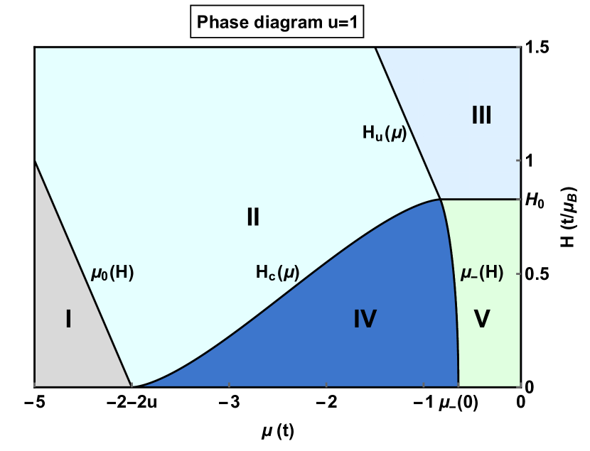
Figure 1: Ground state phase diagram in $\mu-H$ coordinates for $u=1$. The value of $\mu_{-}(0)$ is given by Eq. (13) and $H_{0}(u)=2\left(1+u^{2}\right)^{1/2}-2u$. In terms of the densities and magnetization the five phases are characterized by I: $n=m=0$ , II: $n_{\uparrow}>0\,,n_{\downarrow}=0$, III: $n_{\uparrow}=1\,,n_{\downarrow}=0$, IV: $0<n<1\,,m\geq 0$ and V: $n=1\,,m\geq 0$.

At zero temperature and $\mu\leq 0\,,H\geq 0$ the Hubbard model presents five phases Tak7 ; EFGKK and we should point out that due to the particular form of the Hamiltonian (1) the system is at half filling ($n=1$) for $\mu=0$. For a fixed value of the magnetic field by varying the chemical potential the Hubbard model presents quantum phase transitions at the quantum critical points (QCPs). The universality classes of these QPTs and the associated universal thermodynamics in the vicinity of the QCPs will be studied in Sect. V. The phases can be distinguished by the densities of spin-up and spin-down electrons $n_{\uparrow},n_{\downarrow}$ which serve as order parameters. The five phases and boundaries (which are critical lines of QCPs) are:

• Phase I $(n=m=0)$: Vacuum. This phase is characterized by zero density of electrons and $Q=A=0.$ The boundary is defined by the condition

  $$\mu\leq\mu_{0}(H)=-2-2u-H\,.$$ (10)

  Clearly, all correlation functions are trivial.

• Phase II $(n_{\uparrow}>0\,,n_{\downarrow}=0)$: Partially filled, spin polarized band. The total density is $0<n<1$ and the magnetization $m=n/2$. In this phase the parameter $Q$ can take values between $0$ and $\pi$ and $A=0$. The chemical potential is related to $Q$ and $H$ via

  $$\cos Q=-\frac{1}{2}\left(\mu+H+2u\right)\,,$$

  and the magnetic field satisfies $H_{c}\leq H\leq H_{u}$ with

  $$H_{c} =\frac{2u}{\pi}\int_{0}^{Q}dk\,\cos k\frac{\cos k-\cos Q}{u^{2}+(\sin k)^{2}}\,,$$ (11a)

  $$H_{u} =2-\mu-2u\,.$$ (11b)

  The density is given by $n=\arccos\left(1-\frac{\mu-\mu_{0}(H)}{2}\right)/\pi$.

  Here, the density-density correlation function and the one-particle Green’s function decay algebraically with free fermion exponents, the spin-spin correlation functions are trivial.

• Phase III $(n_{\uparrow}=1\,,n_{\downarrow}=0)$: Half filled, spin polarized band. The total density is $n=1$ and the magnetization is $m=1/2$. The boundaries are given by $(Q=\pi\,,A=0)$

  $$H\geq \,H_{0}(u)=2\left(1+u^{2}\right)^{1/2}-2u\,,$$ (12a)

  $$\mu\geq \,2-2u-H\,.$$ (12b)

  The correlation functions are frozen. Note that the boundaries of phase III in the $\mu-H$ plane are straight lines, the one described by (12a) is strictly horizontal.

• Phase IV $(0<n<1\,,m\geq 0)$: Partially filled and magnetized band. In this phase $0<Q<\pi\,,0<A\leq\infty.$

  The density-density and spin-spin correlation functions as well as the Green’s functions decay algebraically.

• Phase V $(n=1\,,m\geq 0)$: Half filled and magnetized band. In this region $Q=\pi$ and $0<A\leq\infty$. At $H=0$ the value of the chemical potential $\mu_{-}$ which separates phase IV and phase V is given by

  $$\mu_{-}(H=0)=2-2u-2\int_{0}^{\infty}\frac{d\omega}{\omega}\frac{J_{1}(\omega)e^{-\omega u}}{\cosh(\omega u)}\,.$$ (13)

  For $H>0$ the boundary between phase IV and phase V is determined by the condition $\bar{\kappa}(\pm\pi)=0$ (in Eqs. (8) we set $Q=\pi$). As only charge neutral excitations are gapless, the density-density and spin-spin correlation functions decay algebraically, the one-particle Green’s function decays exponentially.

The exponents of the algebraic decay of correlation functions in phases IV and V are given by conformal weights resp. Luttinger liquid parameters that are obtained EFGKK from the dressed charge discussed below in subsection III.3.

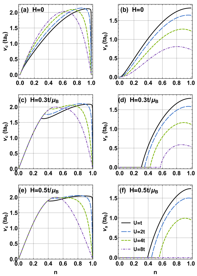
Figure 2: Density dependence of the charge and spin velocities ($a_{0}$ is the lattice spacing) for $H=0$ (upper panels), $H=0.3\,t/\mu_{B}$ (middle panels) and $H=0.5\,t/\mu_{B}$ (bottom panels).

III.2 Spin and charge velocities

The charge and spin velocities can be calculated from

$$v_{c}=\left.\frac{\bar{\kappa}^{\prime}(k)}{2\pi\rho(k)}\right|_{k=Q}\,,\ \ \ v_{s}=\left.\frac{\varepsilon^{\prime}(k)}{2\pi\sigma(\lambda)}\right|_{\lambda=A}\,,$$ (14)

where the derivatives of the dressed energies satisfy the following system of integral equations

$$\bar{\kappa}^{\prime}(k) =2\sin k+\cos k\int_{-A}^{A}d\lambda\,a_{1}(\lambda-\sin k)\varepsilon^{\prime}(\lambda)\,,$$

$$\varepsilon^{\prime}(\lambda) =\int_{-Q}^{Q}dk\,\,a_{1}(\lambda-\sin k)\bar{\kappa}^{\prime}(k)$$

$$\ \ \ \ \ \ \ \ \ \ \ \ \ \ \ \ \ \ \ \ \ \ \ -\int_{-A}^{A}d\lambda^{\prime}a_{2}(\lambda-\lambda^{\prime})\varepsilon^{\prime}(\lambda^{\prime})\,.$$

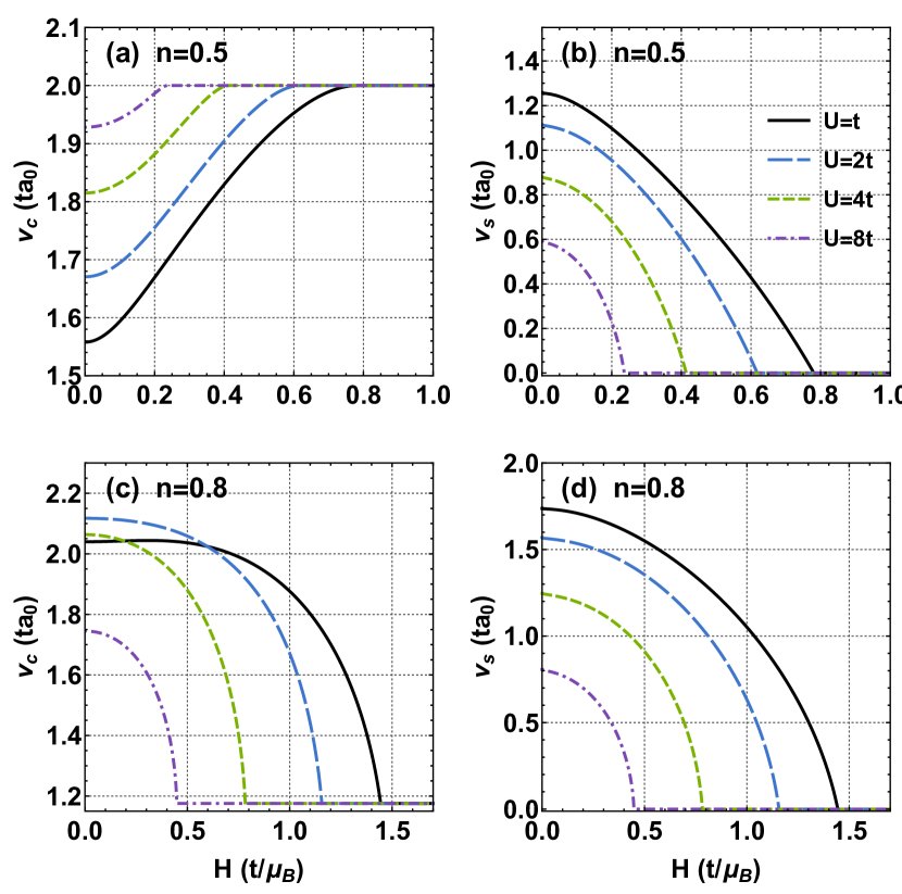
Figure 3: Magnetic field dependence of the charge and spin velocities for two fixed values of the density $n=0.5$ (upper panels) and $n=0.8$ (lower panels). For large values of the magnetic field the charge velocities are $v_{c}(n)=2\sin(\pi n).$

The charge and spin velocities play an important role in the low temperature description of the Hubbard model. In this regime certain phases are described by the TLL theory and the free energy takes the form Hald ; Giamar ; Affleck

$$f_{II} =e_{II}-\frac{\pi T^{2}}{6}\frac{1}{v_{c}}\,,\ \ \mbox{phase II}\,,$$ (15a)

$$f_{IV} =e_{IV}-\frac{\pi T^{2}}{6}\left(\frac{1}{v_{c}}+\frac{1}{v_{s}}\right)\,,\ \ \mbox{phase IV}\,,$$ (15b)

$$f_{V} =e_{V}-\frac{\pi T^{2}}{6}\frac{1}{v_{s}}\,,\ \ \mbox{phase V}\,.$$ (15c)

Therefore, the entropy and the specific heat in phases II, IV and V have a linear dependence on temperature for temperatures close to zero and the slope (also known as the specific heat coefficient) can be determined from the knowledge of the velocities.

The dependence of the velocities on the filling factor at zero and nonzero magnetic field is presented in Fig. 2. To our knowledge the only result reported in the literature (see Schulz1 and Chap. VI of EFGKK ) is the case of zero magnetic field which is presented in the panels (a) and (b) of Fig. 2. The charge velocity is zero at both $n=0$ and $n=1$ signalling the quantum phase transitions between phases I and IV and IV and V (for $H=0$ and $0<n<1$ the system is in phase IV). For weak interactions $v_{c}$ presents a rapid variation close to half filling. The spin velocity is zero only at $n=0$ and reaches a finite value at $n=1$.

The presence of a magnetic field introduces additional complications. For small values of $n$ and $H>0$ the system is fully polarized (phase II, $A=0$) and from Eqs. (3) and (8) we have $\rho(k)=1/2\pi$ and $\bar{\kappa}(k)=-2\cos k-\mu-2u-H$. Together with Eq. (5) and the definitions (14) they imply that in phase II $v_{c}=2\sin(\pi n)$ and $v_{s}=0$. For every value of $U$ and $H<H_{0}(U)$ there is a critical value of $n$ at which the system crosses in phase IV and $v_{s}$ becomes nonzero. The charge velocity is continuous at this critical value of density but the derivative is discontinuous. Numerical results for the velocities in the presence of a magnetic field are presented in panels (c)–(f) of Fig. 2. For $H=0.3$ and $U=\{1,2,4,8\}$ the transition from phase II to IV can be seen clearly in the discontinuity of the derivative of $v_{c}$ which coincides with the value of $n$ for which $v_{s}$ becomes nonzero (see panels (c) and (d) of Fig. 2). For $H=0.5$ and $U=8$ we have $H>H_{0}(8)=0.4721\ldots$ and for these values of the magnetic field and interaction strength the system is found in phase II for all densities which means that $v_{c}=2\sin(\pi n)$ and $v_{s}=0$ for $n\in[0,1]$. This can be seen in panels (e) and (f) of Fig. 2.

Fig. 3 presents the dependence of the spin and charge velocities on magnetic field at fixed density. Here at low values of $H$ the system is found in phase IV and as the magnetic field is increased we cross into phase II for which $v_{c}=2\sin(\pi n)$ and $v_{s}=0$.

At half filling only the spin degrees of freedom are gapless and $v_{c}=0$. The dependence of the spin velocity at half filling as a function of the magnetic field is presented in Fig. 4. $v_{s}$ is monotonically decreasing as $H$ is increased and vanishes like $(H_{0}(U)-H)^{1/2}$ in the vicinity of $H_{0}(u)=2\left(1+u^{2}\right)^{1/2}-2u$. Another interesting feature is the logarithmic behaviour $v_{s}(H)\sim v_{s}(0)+a/\log(H/H_{0})$ for small values of $H$ as it can be seen in the right panels of Fig. 4.

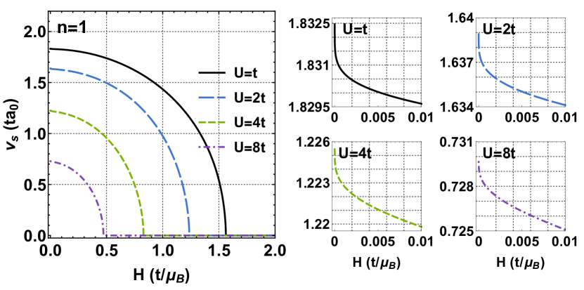
Figure 4: (Left panel) The spin velocity at half filling as a function of the magnetic field for different values of $U$. In the vicinity of $H_{0}(U)$ the velocity behaves like $v_{s}\sim(H_{0}(U)-H)^{1/2}$. (Right panels) The logarithmic behavior of the spin velocity at small values of $H$.

III.3 Susceptibilities at zero temperature

The spin and charge susceptibilities in the grand-canonical ensemble are defined as

$$\chi(\mu,H)=2\,\frac{\partial m}{\partial H}\,,\ \ \ \kappa(\mu,H)=\frac{\partial n}{\partial\mu}\,.$$ (16)

Below we list known analytical formulae for the susceptibilities in each of the five phases at zero temperature. Our presentation follows Chap. VI of EFGKK (we should point out that our spin susceptibility contains an additional factor of 2 compared with the definition employed in EFGKK ).

• Phases I and III. In these phases the spin and charge susceptibilities are both zero.

• Phase II. The system is fully polarized with density $n=\arccos\left(1-\frac{\mu-\mu_{0}(H)}{2}\right)/\pi$ and

  $$\kappa(\mu,H)=\frac{1}{\pi v_{c}}=\frac{1}{\pi\left(4-(\mu+2u+H)^{2}\right)^{1/2}}\,.$$ (17)

  Note that $\kappa(\mu,H)$ and the grand-canonical spin susceptibility $\chi(\mu,H)$ are identical, implying that the canonical spin susceptibility is zero.

• Phase IV. We introduce an important quantity called the dressed charge matrix and defined by (Woyn0 ; IKR ; FY ; FK1 ; FK2 and Chap. VIII of EFGKK )

  $$Z=\left(\begin{array}[]{lr}Z_{cc}&Z_{cs}\\ Z_{sc}&Z_{ss}\end{array}\right)=\left(\begin{array}[]{lr}\xi_{cc}(Q)&\xi_{cs}(A)\\ \xi_{sc}(Q)&\xi_{ss}(A)\end{array}\right)\,,$$ (18)

  where $\xi_{ab}(k)\,,\ a,b\in\{c,s\}$ satisfy the system of integral equations

  $$\xi_{cc}(k) =1+\int_{-A}^{A}d\lambda^{\prime}\,\xi_{cs}(\lambda^{\prime})a_{1}(\lambda^{\prime}-\sin k)\,,$$ (19a)

  $$\xi_{cs}(\lambda) =\int_{-Q}^{Q}dk\,\cos k^{\prime}\xi_{cc}(k^{\prime})a_{1}(\sin k^{\prime}-\lambda)$$

  $$\ \ \ \ \ \ \ \ \ \ \ \ \ \ \ \ -\int_{-A}^{A}d\lambda^{\prime}\xi_{cs}(\lambda^{\prime})a_{2}(\lambda^{\prime}-\lambda)\,,$$ (19b)

  $$\xi_{sc}(k) =\int_{-A}^{A}d\lambda^{\prime}\xi_{ss}(\lambda^{\prime})a_{1}(\lambda^{\prime}-\sin k)\,,$$ (19c)

  $$\xi_{ss}(\lambda) =1+\int_{-Q}^{Q}dk^{\prime}\cos k^{\prime}\xi_{sc}(k^{\prime})a_{1}(\sin k^{\prime}-\lambda)$$

  $$\ \ \ \ \ \ \ \ \ \ \ \ \ \ \ \ -\int_{-A}^{A}d\lambda^{\prime}\xi_{ss}(\lambda^{\prime})a_{2}(\lambda^{\prime}-\lambda)\,.$$ (19d)

  The susceptibilities are expressed in terms of the elements of dressed charge matrix and velocities as

  $$\chi(\mu,H) =\frac{(Z_{cs}-2Z_{ss})^{2}}{2\pi v_{s}}+\frac{(Z_{cc}-2Z_{sc})^{2}}{2\pi v_{c}}\,,$$ (20)

  $$\kappa(\mu,H) =\frac{Z_{cc}^{2}}{\pi v_{c}}+\frac{Z_{cs}^{2}}{\pi v_{s}}\,.$$ (21)

• Phase V. At half filling and magnetization $m<1/2$ we have

  $$\chi(H,n=1)=\frac{4\xi_{s}^{2}(A)}{\pi v_{s}}\,,\ \ \ \kappa(H,n=1)=0\,,$$ (22)

  where $\xi_{s}(A)$ is the dressed charge for the half filled band and satisfies the integral equation

  $$\xi_{s}(\lambda)=1-\int_{-A}^{A}d\lambda^{\prime}\,a_{2}(\lambda-\lambda^{\prime})\xi_{s}(\lambda^{\prime})\,.$$ (23)

IV Thermodynamics at finite temperature

The first thermodynamic description of the Hubbard model was derived by Takahashi in the framework of TBA and assuming the string hypothesis Tak6 . While extremely important the infinite system of non-linear integral equations derived using this method is very hard to implement numerically. For this reason in this paper we are going to investigate the thermodynamic properties of the Hubbard model using the quantum transfer matrix formalism Suz ; SI ; Koma ; SAW ; K1 ; K2 which has the advantage of providing a thermodynamic description involving a finite number of auxiliary functions JKS . More precisely we employ only 6 auxiliary functions denoted by $\mathfrak{b}^{\pm}\,,\mathfrak{c}^{\pm}$ and $\overline{\mathfrak{c}^{\pm}}\,,$ and we define

$$\mathfrak{B}^{\pm}:=1+\mathfrak{b}^{\pm}\,, \ \ \ \overline{\mathfrak{B}^{\pm}}:=1+1/\mathfrak{b}^{\pm}\,,$$

$$\mathfrak{C}^{\pm}:=1+\mathfrak{C}^{\pm}\,, \ \ \ \overline{\mathfrak{C}^{\pm}}:=1+\overline{\mathfrak{c}^{\pm}}\,,$$

$$\Delta\ln\mathfrak{C}:=\ln(\mathfrak{C}^{+}/\mathfrak{C}^{-})\,,\ \ \ \ \Delta\ln\overline{\mathfrak{C}}:=\ln(\overline{\mathfrak{C}^{+}}/\overline{\mathfrak{C}^{-}})\,.$$

These functions satisfy the following system of nonlinear integral equations derived in JKS

$$\ln\mathfrak{b}^{\pm} =-\beta H-K_{2,\pm\alpha-\alpha}*\ln\mathfrak{B}^{+}+K_{2,\pm\alpha+\alpha}*\ln\mathfrak{B}^{-}$$

$$\ \ \ \ \ \ \ \ \ \ \ \ \ \ \ \ \ \ \ \ \ -\overline{K}_{1,\pm\alpha}\bullet\Delta\ln(\overline{\mathfrak{c}}/\overline{\mathfrak{C}})\,,$$ (24a)

$$\ln\mathfrak{c}^{\pm} =\Psi_{c}^{\pm}+\overline{K}_{1,-\alpha}*\ln\overline{\mathfrak{B}^{+}}-\overline{K}_{1,\alpha}*\ln\overline{\mathfrak{B}^{-}}$$

$$\ \ \ \ \ \ \ \ \ \ \ \ \ \ \ \ \ \ \ \ \ +\overline{K}_{1,0}\bullet\Delta\ln\overline{\mathfrak{C}}\pm\frac{1}{2}\Delta\ln\overline{\mathfrak{C}}\,,$$ (24b)

$$\ln\overline{\mathfrak{c}^{\pm}} =\overline{\Psi}_{c}^{\pm}-K_{1,-\alpha}*\ln\mathfrak{B}^{+}+K_{1,\alpha}*\ln\mathfrak{B}^{-}$$

$$\ \ \ \ \ \ \ \ \ \ \ \ \ \ \ \ \ \ \ \ \ -K_{1,0}\bullet\Delta\ln\mathfrak{C}\pm\frac{1}{2}\Delta\ln\mathfrak{C}\,,$$ (24c)

where $u=U/4\,,\ 0<\alpha<u\,,f_{\alpha}(x)=f(x+i\alpha)$ and

$$K_{1}(x) =\frac{u/\pi}{x(x+2iu)}\,,$$ (25a)

$$\overline{K}_{1}(x) =\frac{u/\pi}{x(x-2iu)}\,,$$ (25b)

$$K_{2}(x) =\frac{2u/\pi}{x^{2}+4u^{2}}\,.$$ (25c)

The driving terms are

$$\Psi_{c}^{\pm}(x) =-\beta U/2+\beta(\mu+H)+\ln\phi_{\pm 0}(x)\,,$$ (26)

$$\overline{\Psi}_{c}^{\pm}(x) =-\beta U/2-\beta(\mu+H)-\ln\phi_{\pm 0}(x)\,,$$ (27)

$$\ln\phi_{\pm 0}(x) =\pm 2\beta(1-x^{2})^{1/2}\,,$$ (28)

and the two types of convolutions appearing in Eqs. (24) are defined by

$$K*f =\int_{-\infty}^{+\infty}K(x-y)f(y)\,dy\,,$$ (29)

$$K\bullet f =\mbox{p.v.}\int_{-1}^{+1}K(x-y)f(y)\,dy\,,$$ (30)

where p.v. denotes the principal value integral. The grandcanonical potential of the system can be obtained from

$$- \beta\phi(\mu,H,T,U)=\beta(\mu+H/2+U/4)$$

$$-\int_{-1}^{+1}\mathcal{K}\ln[(1+\mathfrak{c}^{+}+\overline{\mathfrak{c}^{+}})(1+\mathfrak{c}^{-}+\overline{\mathfrak{c}^{-}})]\,dx$$

$$+\int_{-\infty}^{+\infty}[(\mathcal{K}_{\alpha-2u}-\mathcal{K}_{\alpha})\ln\mathfrak{B}^{+}$$

$$\ \ \ \ \ \ \ \ \ \ \ \ \ \ \ \ \ \ \ -(\mathcal{K}_{-\alpha-2u}-\mathcal{K}_{-\alpha})\ln\mathfrak{B}^{-}]\,dx$$

with $\mathcal{K}(x)=-[2\pi(1-x^{2})^{1/2}]^{-1}$. In the noninteracting case, $U=0$, the grandcanonical potential is known analytically

$$\phi_{FF}(\mu,H,T)=-\frac{T}{2\pi}\int_{-\pi}^{\pi}dk\,\ln\left[1+e^{\frac{2\cos k-\mu-H}{T}}\right]$$

$$\ \ \ \ \ \ \ \ \ \ \ \ \ \ \ \ \ \ \ -\frac{T}{2\pi}\int_{-\pi}^{\pi}dk\,\ln\left[1+e^{\frac{2\cos k-\mu+H}{T}}\right]\,,$$ (31)

and in the limit of infinite repulsion we have Tak1

$$\phi_{\infty}(\mu,H,T)=$$

$$\ \ \ \ -\frac{T}{2\pi}\int_{-\pi}^{\pi}dk\,\ln\left[1+2\cosh\left(\frac{H}{T}\right)e^{\frac{2\cos k-\mu}{T}}\right]\,.$$ (32)

The integral equations (24) can be solved by a simple iterative procedure. First, we make an initial guess of the six functions, which are then plugged into the right hand side of (24) obtaining an approximate solution. This process is iterated until the difference between the functions obtained in two successive steps is smaller than a given error. This algorithm requires an efficient numerical treatment of the two types of convolutions appearing in the integral equations which is detailed in Appendices A and B. Another difficulty lies in the fact that while for the first type of convolution we use the Fast Fourier Transform for the second type we use a Chebyshev quadrature which means that the six functions are discretized on different grids requiring the use of interpolation at each iterative step.

V Quantum critical behaviour

At low temperatures the Hubbard model shows thermodynamically activated behaviour in the gapped phases I and III, and algebraic dependence on temperature in the gapless phases II, IV and V, see (15). The various types of behaviour hold inside the phases. At the boundaries – here referred to as quantum critical lines – rather complex crossover behaviour is observed which is one of the main objectives of this paper.

The Hubbard model presents a multitude of quantum phase transitions and quantum critical lines. The effects of the QPTs can be measured at low but finite temperatures in the quantum critical (QC) region which is characterized by strong coupling of quantum and thermal fluctuations Sachdev . In the vicinity of the quantum critical points the thermodynamics is expected to be universal and determined by the universality class of the transition. For example, in the case of a QPT induced by the variation of the chemical potential at fixed magnetic field the pressure is assumed to satisfy ZH

$$p(\mu,H,T)\sim p_{r}(\mu,H,T)+T^{\frac{d}{z}+1}\mathcal{P}_{H}\left(\frac{\mu-\mu_{c}(H)}{T^{\frac{1}{\nu z}}}\right)\,,$$ (33)

with $p_{r}$ the regular part of the pressure, $d$ the dimension, $\mathcal{P}_{H}$ a universal function and $\mu_{c}(H)$ the quantum critical point. The correlation length exponent $\nu$ and the dynamical critical exponent $z$ determine the universality class of the transition. Other relevant thermodynamic quantities can be derived from (33) using thermodynamic identities.

The universality class of a QPT can be determined by plotting the “scaled” quantity $(p(\mu,H,T)-p_{r}(\mu,H,T))T^{-\frac{d}{z}-1}$ (or other suitable thermodynamic function) as a function of the chemical potential and for several values of temperature ZH . If the $z$ and $\nu$ exponents are chosen correctly then all the curves intersect at $\mu_{c}(H).$ It is efficient to choose a thermodynamic parameter for which the regular part is known from previous theoretical considerations. Plotting the “scaled” quantities as functions of $(\mu-\mu_{c}(H))/T^{\frac{1}{\nu z}}$ all curves collapse to the universal function $\mathcal{P}_{H}$.

V.1 QPTs induced by the variation of the chemical potential at zero magnetic field

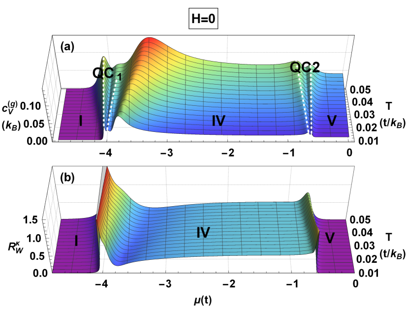
Figure 5: (a) Chemical potential and temperature dependence of the grandcanonical specific heat for $U=4\,t$ and zero magnetic field. The boundaries of the critical regions identified with the maxima of $c_{V}^{(g)}$ are highlighted by dashed white lines. The two QCPs are $\mu_{c}^{(I\rightarrow IV)}=-4\,t$ and $\mu_{c}^{(IV\rightarrow V)}\equiv\mu_{-}(0)=-0.6433\,t\,.$ (c) Chemical potential and temperature dependence of the Wilson ratio $R_{W}^{\kappa}$. Note the anomalous enhancement in the quantum critical regions.

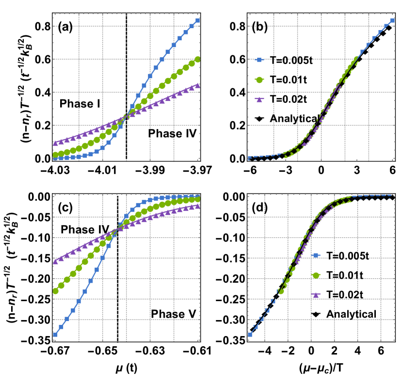
Figure 6: Plots of the scaled densities $(n-n_{r})T^{-1/2}$ as functions of the chemical potential at different temperatures in the vicinities of the QCPs: $\mu_{c}^{(I\rightarrow IV)}=-4\,t$ (a) and $\mu_{c}^{(IV\rightarrow V)}=-0.6433\,t$ (c). For the first transition $n_{r}=0$ and for the second $n_{r}=1$. The dashed vertical lines pass through the QCPs. Plotting the scaled densities as functions of $(\mu-\mu_{c})/T$ all curves collapse to the universal function $\mathcal{P}_{H}^{\prime}(x)$ (b) for the first transition and (d) for the second transition. In panels (b) and (d) the black diamonds represent the analytical predictions for the universal function $\mathcal{P}_{H}^{\prime}(x)$ obtained from the derivative of Eq. (36) (b) and Eq. (37) (d) with $a=0.462$ and $b=-1$.

We will first investigate the QPTs induced by the variation of the chemical potential at zero magnetic field. In the attractive case a similar analysis can be found in CYBG0 ; CYBG . In addition to the determination of the QCPs and the universality class of the transitions a problem of considerable importance is represented by the identification of the boundaries of the QC regions. It was argued recently HJYLG ; YCZSG ; BGKRT ; PKF ; PK that the grandcanonical specific heat $c_{V}^{(g)}=-T\left(\partial^{2}\phi/\partial T^{2}\right)_{\mu,H}$ can be used for this task. The specific heat presents two lines of local maxima fanning out from the QCP and the location of these maxima can be identified with the boundaries of the QC region. Another useful quantity which can be used to distinguish the various phases at low temperatures YCLRG is the compressibility Wilson ratio defined by

$$R_{W}^{\kappa}=\frac{\pi^{2}}{3}T\frac{\kappa}{c_{V}^{(g)}}\,.$$ (34)

where $\kappa$ is the compressibility of the system. In Fig. 5 we present the dependence of the grandcanonical specific heat and compressibility Wilson ratio on chemical potential and temperature for $U=4$ and $H=0$. The system presents two QPTs between phases I and IV with critical point $\mu_{c}^{(I\rightarrow IV)}=-2u-2=-4$ and between phases IV and V with $\mu_{c}^{(IV\rightarrow V)}\equiv\mu_{-}(0)=-0.6433\,$ ($\mu_{-}(0)$ is given by Eq. (13)). The boundaries of both critical regions can be identified with the lines of maxima of the specific heat fanning out from the critical points. The Wilson ratio presents anomalous enhancements in the QC regions and is almost constant in the other regimes.

The identification of the universality classes of the QPTs is done by employing the scaling relation for the density which at zero temperature is zero in phase I and one in phase V. Taking the derivative with respect to $\mu$ of Eq. (33) we obtain

$$n(\mu,H,T)\sim\frac{\partial p_{r}}{\partial\mu}(\mu,H,T)+T^{\frac{d}{z}+1-\frac{1}{\nu z}}\mathcal{P}_{H}^{\prime}\left(\frac{\mu-\mu_{c}(H)}{T^{\frac{1}{\nu z}}}\right)\,.$$

The curves $(n-n_{r})T^{-\frac{d}{z}-1+\frac{1}{\nu z}}$ with $n_{r}=\partial p_{r}/\partial\mu=0$ for the first transition and $n_{r}=1$ for the second transition intersect at the critical points $\mu_{c}$ when the critical exponents are $z=2$ and $\nu=1/2$ as it can be seen in Fig. 6.

Even though both QPTs are characterized by the same critical exponents the universal thermodynamics in the vicinity of the QCPs is not given by the same universal function $\mathcal{P}_{H}(x).$ For the transition between phases I to IV we can analytically derive the universal function as follows. Close to the first critical point the system is characterized by very low densities and it is equivalent to the repulsive Gaudin-Yang model (two component fermions with repulsive delta-interaction). For this continuum model the QPT between the vacuum and the TLL phase belongs to the universality class of spin-degenerate impenetrable particle gas PKF with the universal thermodynamics described by Takahashi’s formula Tak1 ($x=[\mu-\mu_{c}(H)]/T\,,y=H/T$)

$$p=\frac{T^{3/2}}{2\pi}\int_{-\infty}^{+\infty}\ln\left[1+(1+e^{-2|y|})e^{-k^{2}+x}\right]\,dk\,.$$ (35)

For $H=0$ we have $e^{-2|y|}=1$ and

$$\mathcal{P}_{H}(x)=\frac{1}{2\pi}\int_{-\infty}^{+\infty}\ln\left[1+2e^{-k^{2}+x}\right]\,dk\,.$$ (36)

A comparison of the numerical data with the analytical predictions of Eq. (36) can be seen in Fig. 6 (b) which confirms the validity of our analytical derivation. Eq. (36) is valid for all $U>0$. In the case of free fermions on the lattice the system still presents a QPT between the vacuum and the partially filled and magnetized band phase with the QCP $\mu_{c}(H)=-2-H$ (see Chap. 6.1 of EFGKK ) with the thermodynamics described by the free fermionic formula.

We should point out that the QC regions have physical properties which are different from the ones of the surrounding phases, particularly in the case of the correlation functions. For example, at low temperatures, phase I can be well described by a dilute classical gas in which thermal effects play an important role while in phase IV the quantum effects dominate and the system is described by a two-component TLL. In the QC region between phases I and IV both quantum and thermal effects are important producing distinct correlation functions.

As we will show below all the other QPTs investigated in this paper have critical exponents $z=2$ and $\nu=1/2$ and therefore it is sensible to assume that the scaling of the pressure for these transitions is given by $p=T^{3/2}\mathcal{P}(x)$ with the universal function

$$\mathcal{P}(x)=\frac{a}{2\pi}\int_{-\infty}^{+\infty}\ln\left[1+e^{-k^{2}+b\,x}\right]\,dk\,,$$ (37)

where $a$ and $b$ are free parameters and $x=(\mu-\mu_{c}(H))/T$ for the chemical potential induced QPTs and $x=(H-H_{c}(\mu))/T$ for the magnetic field ones. The parameter $a$ takes some positive real number and is related to the square root of the mass of the particle with parabolic energy-momentum dispersion. The parameter $b$ describes the strength of the coupling of the external field, chemical potential or magnetic field, to some particle number and typically takes values $\pm 1$ for particle and hole type excitations and $\pm 2$ for magnetic excitations: a change of the particle number carries energy $\pm\mu$ and a spin-flip results in $\pm 2H$, see (2c). An exception is realized by the phase transition from II to IV where particles with parabolic dispersion enter the system on a background of majority particles with finite density. There the Hubbard interaction leads to an effective parameter $b$ different from -1.

For the transition between phases IV and V the best fit is obtained for $a=0.462$ and $b=-1$ and is shown in panel (d) of Fig. 6.

V.2 QPTs induced by the variation of the chemical potential at nonzero magnetic field

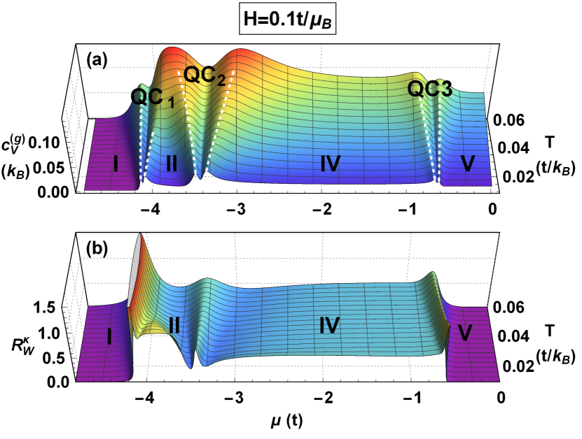
Figure 7: (a) Chemical potential and temperature dependence of the grandcanonical specific heat for $U=4t$ and $H=0.1\,t/\mu_{B}$. The boundaries of the critical regions identified with the maxima of $c_{V}^{(g)}$ are highlighted by dashed white lines. The three QCPs are $\mu_{c}^{(I\rightarrow II)}=-2u-2-H=-4.1\,t\,,$ $\mu_{c}^{(II\rightarrow IV)}=-3.429\,t\,$ and $\mu_{c}^{(IV\rightarrow V)}=-0.6453\,t$. (b) Chemical potential and temperature dependence of the Wilson ratio $R_{W}^{\kappa}$.

In the presence of a magnetic field the repulsive Hubbard model presents three QPTs induced by the variation of the chemical potential. It can be seen in Fig. 7 for $U=4$ and $H=0.1$ that the specific heat presents two lines of maxima to the left and right of each QCP and that the Wilson ratio also presents maxima in each quantum critical region while being almost constant outside of them. The values of the three QCPs are: $\mu_{c}^{(I\rightarrow II)}=-2u-2-H=-4.1\,,$ $\mu_{c}^{(II\rightarrow IV)}=-3.429\,$ and $\mu_{c}^{(IV\rightarrow V)}=-0.6453$.

For the determination of the critical exponents we use the scaling of the densities for the I $\rightarrow$ II and IV $\rightarrow$ V transitions ($n_{r}$(phase I)=0 and $n_{r}$(phase V)=1) and the density of down spins for the II $\rightarrow$ IV transition ($n_{\downarrow,r}$(phase II)=0). Using $n_{\downarrow}=-(\partial\phi/\partial\mu+\partial\phi/\partial H)/2$ we find

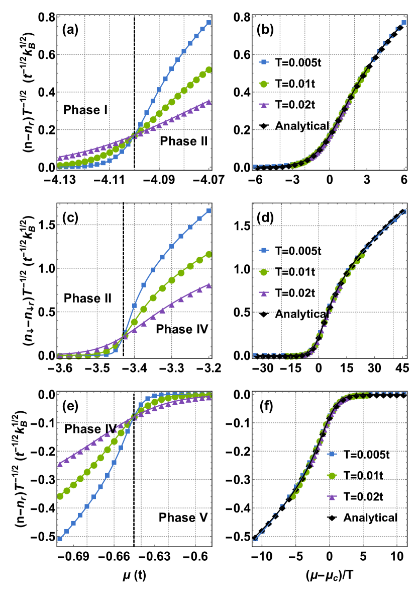
Figure 8: Plots of the scaled total densities $(n-n_{r})T^{-1/2}$ and density of down spins $(n_{\downarrow}-n_{\downarrow r})T^{-1/2}$ as functions of the chemical potential at different temperatures in the vicinities of the QCPs $\mu_{c}^{(I\rightarrow II)}=-4.1\,t$ (a), $\mu_{c}^{(II\rightarrow IV)}=-3.429\,t\,$ (c) and $\mu_{c}^{(IV\rightarrow V)}=-0.6453\,t$ (e). The regular parts are $n_{r}$(phase I)=0, $n_{\downarrow,r}$(phase II)=0 and $n_{r}$(phase V)=1. The dashed vertical lines pass through the QCPs. Plotting the scaled quantities as functions of $(\mu-\mu_{c})/T$ all curves collapse to the universal functions $\mathcal{P}_{H}^{\prime}(x)$ (b), (d) and (f). In panel (b) the black diamonds represent the analytical predictions for the universal function $\mathcal{P}_{H}^{\prime}(x)$ obtained from the derivative of Eq. (38). In panels (d) and (f) the analytical predictions for the universal functions are obtained from Eq. (37) with $a=3.1\,,b=0.4$ (d) and $a=0.476\,,b=-1$ (f).

$$n_{\downarrow}(\mu,H,T)\sim n_{\downarrow,r}(\mu,H,T)$$

$$\ \ \ \ \ \ \ \ \ \ +\frac{(1-\mu_{c}^{\prime}(H))}{2}T^{\frac{d}{z}+1-\frac{1}{\nu z}}\mathcal{P}_{H}^{\prime}\left(\frac{\mu-\mu_{c}(H)}{T^{\frac{1}{\nu z}}}\right)\,.$$

For all QPTs the critical exponents are $z=2$ and $\nu=1/2$ as it can be seen from Fig. 8. Similar to the previous case, even though the critical exponents are the same the universal function $\mathcal{P}_{H}(x)$ seems to be different for each QPT. For the I $\rightarrow$ II transition from Eq. (35) ($e^{-2|y|}\sim 0$ at low temperatures) the universal function at finite magnetic field is

$$\mathcal{P}_{H}(x)=\frac{1}{2\pi}\int_{-\infty}^{+\infty}\ln\left[1+e^{-k^{2}+x}\right]\,dk\,.$$ (38)

In panel (b) of Fig. 8 it is shown that this analytical formula agrees perfectly with the numerical data. Together with the previous result this proves that the transition I $\rightarrow$ IV belongs to the universality class of the spin-degenerate impenetrable particle gas which is characterized by Takahashi’s formula Eq. (35). The transition I $\rightarrow$ II belongs to the strong field limit of the spin-degenerate impenetrable particle gas and is better known as simply the impenetrable particle gas.

For the II to IV and IV to V transitions the best fits for the universal function are obtained using Eq. (37) with $a=3.1\,,b=0.4$ (II $\rightarrow$ IV) and $a=0.476\,,b=-1$ (IV $\rightarrow$ V) as it can be seen in panels (d) and (f) of Fig. 8.

V.3 QPTs induced by the variation of the magnetic field at half filling

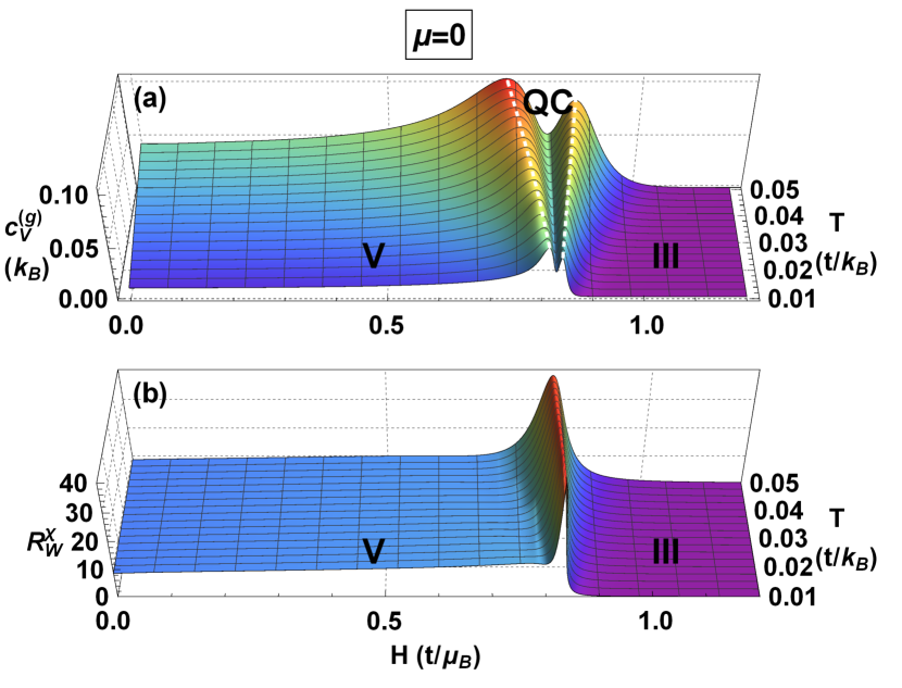
Figure 9: (a) Magnetic field and temperature dependence of the grandcanonical specific heat for $U=4t$ at half filling ($\mu=0$). The boundaries of the critical region identified with the maxima of $c_{V}^{(g)}$ are highlighted by dashed white lines. The QCP is $H_{c}^{(V\rightarrow III)}\equiv H_{0}(U)=0.8284\,t/\mu_{B}\,.$ (b) Magnetic field and temperature dependence of the Wilson ratio $R_{W}^{\chi}$.

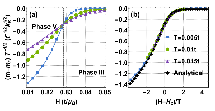
Figure 10: (a) Plot of the scaled magnetization $(m-m_{r})T^{-1/2}$ versus magnetic field at different temperatures in the vicinity of the QCP $H_{c}^{(V\rightarrow III)}\equiv H_{0}(U)=0.8284\,t/\mu_{B}\,.$ The regular part of the magnetization is $m_{r}$(phase III)=$1/2.$ (b) Universal function $\mathcal{P}_{\mu}^{\prime}(x)$ obtained from the collapse of all the curves plotted as functions of $(H-H_{c})/T$. The black diamonds represent the analytical predictions for the universal function $\mathcal{P}_{\mu}^{\prime}(x)$ obtained from the derivative of Eq. (37) for $a=0.8$ and $b=-2$.

The Hubbard model also presents QPTs induced by the variation of the magnetic field when the chemical potential is fixed. The most interesting is the transition between phases V and III at half filling. For magnetically induced phase transitions the scaling relation (33) becomes

$$p(\mu,H,T)\sim p_{r}(\mu,H,T)+T^{\frac{d}{z}+1}\mathcal{P}_{\mu}\left(\frac{H-H_{c}(\mu)}{T^{\frac{1}{\nu z}}}\right)\,.$$ (39)

Also in this case the relevant dimensionless ratio is the susceptibility Wilson ratio GYFBL defined by

$$R_{W}^{\chi}=\frac{4}{3}\pi^{2}T\frac{\chi}{c_{V}^{(g)}}\,,$$ (40)

where $\chi$ is the magnetic susceptibility. The dependence on the magnetic field and temperature of the grand canonical specific heat and Wilson ratio $R_{W}^{\chi}$ for $U=4$ and $\mu=0$ is presented in Fig. 9. The specific heat presents lines of maxima which define the boundaries of the CR and the Wilson ratio presents anomalous enhancement in the vicinity of the QCP defined by $H_{c}\equiv H_{0}(U)=0.8284$ ($H_{0}(U)$ is defined in Eq. (12a). The scaling of the magnetization which satisfies

$$2m(\mu,H,T)\sim m_{r}(\mu,H,T)+T^{\frac{d}{z}+1-\frac{1}{\nu z}}\mathcal{P}_{\mu}^{\prime}\left(\frac{H-H_{c}(\mu)}{T^{\frac{1}{\nu z}}}\right)\,,$$

is presented in Fig. 10 ($m_{r}$(phase III)=1/2). The critical exponents of this transition are also $z=2$ and $\nu=1/2$.

The universal function is given by Eq. (37) with $a=0.8$ and $b=-2$. The value for $b$ agrees with the one obtained in CYBG for the attractive Hubbard model. It should be noted that the connection between the thermodynamics of the repulsive and attractive model is given by (see Chap. II of EFGKK )

$$\phi(\mu,H,T,u)=\phi(H,\mu,T,-u)-\mu+H\,,$$ (41)

and the equivalent transition in the attractive case is a chemical potential induced one (I to V in the terminology of CYBG and their $x$ is $-x$ in Eq. (37)).

VI Thermodynamic properties below half filling

Figure 11: Temperature dependence of the specific heat in zero magnetic field for various filling fractions and interaction strengths.

In this Section we will investigate the effect of the magnetic field on the thermodynamic properties of the repulsive Hubbard model below half filling, $n\in[0,1)$. We will mainly focus on the canonical specific heat, the grand canonical magnetic susceptibility and compressibility defined by

$$c_{V}^{(c)} =-T\left[\left(\frac{\partial^{2}\phi}{\partial T^{2}}\right)_{\mu,H}+\left(\frac{\partial n}{\partial T}\right)_{\mu,H}^{2}\left(\frac{\partial n}{\partial\mu}\right)_{T,H}^{-1}\right]\,,$$ (42)

$$\chi =-\left(\frac{\partial^{2}\phi}{\partial H^{2}}\right)_{\mu,T}\,,$$ (43)

$$\kappa =-\left(\frac{\partial^{2}\phi}{\partial\mu^{2}}\right)_{H,T}\,.$$ (44)

The thermodynamic properties of the system with $n\in(1,2]$ are related to similar quantities below half filling using the following symmetry of the grand canonical potential (Chap. II of EFGKK )

$$\phi(\mu,H,T,u)+\mu=\phi(-\mu,H,T,u)-\mu\,.$$ (45)

(Note that this elegant symmetry relation is literally satisfied if we extend in (2c) the term $\mu(n_{j,\uparrow}+n_{j,\downarrow})$ to $\mu(n_{j,\uparrow}+n_{j,\downarrow}-1)$.) For the densities and magnetization we find $(\mu\geq 0\,,H\geq 0)$

$$n(\mu) =2-n(-\mu)\,,\ \ m(\mu)=m(-\mu)\,,$$ (46a)

$$n_{\uparrow}(\mu) =1-n_{\downarrow}(-\mu)\,,\ \ n_{\downarrow}(\mu)=1-n_{\uparrow}(-\mu)\,,$$ (46b)

which shows that for our Hamiltonian (1) the system is at half filling for $\mu=0$. From Eq. (45) the connection between the thermodynamic quantities below and above half filling is given by $(n\in[0,1))$

$$c_{V}^{(c)}(n)=c_{V}^{(c)}(2-n)\,,\ \chi(n)=\chi(2-n)\,,\ \kappa(n)=\kappa(2-n)\,.$$ (47)

VI.1 Specific heat

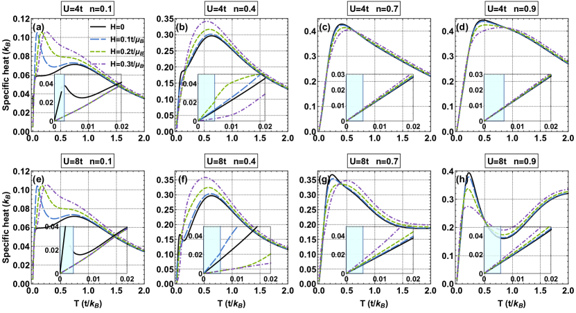
Figure 12: Temperature dependence of the specific heat in the presence of a magnetic field. The insets present a zoom of the data at low temperatures. The shaded regions contain the theoretical predictions $c_{V}^{(c)}=\gamma T$ with specific heat coefficients given in Tables 1 and 2.

The first numerical investigations of the specific heat were performed by Shiba and Pincus Shiba1 ; Shiba2 who considered finite chains for up to 6 lattice sites at half filling. The low-temperature properties for the entire phase diagram were studied by Takahashi Tak7 using the TBA equations Tak6 . For small temperatures the specific heat in phases II, IV and V is linear in $T$ and in phases I and III it behaves like $T^{3/2}e^{-\alpha/T}$. On the critical lines $c_{V}^{(c)}$ is proportional to $T^{1/2}.$ The specific heat coefficient which characterizes the linear dependence on the temperature ($c_{V}^{(c)}\sim\gamma\,T$) is given by

$$\gamma_{II} =\frac{\pi}{3}\frac{1}{v_{c}}\,,\ \ \mbox{phase II}\,,$$ (48a)

$$\gamma_{IV} =\frac{\pi}{3}\left(\frac{1}{v_{c}}+\frac{1}{v_{s}}\right)\,,\ \ \mbox{phase IV}\,,$$ (48b)

$$\gamma_{V} =\frac{\pi}{3}\frac{1}{v_{s}}\,,\ \ \mbox{phase V}\,.$$ (48c)

with $v_{c,s}$ the charge and spin velocities. Numerical investigations of the specific heat using the TBA equations can be found in UKO2 ; KUO1 ; Ha . At zero magnetic field extensive results derived using the QTM thermodynamics (24) can be found in JKS and Chap. XIII of EFGKK . At low temperatures the grand canonical specific heat $c_{V}^{(g)}=-T\left(\frac{\partial^{2}\phi}{\partial T^{2}}\right)_{\mu,H}$ and the canonical specific heat $c_{V}^{(c)}$ are very similar but at high temperatures differences appear.

Specific heat coefficients $U=4$
$\gamma$	H=0	H=0.1	H=0.2	H=0.3
n=0.1	14.60 [IV]	1.694 [II]	1.694 [II]	1.694 [II]
n=0.4	2.183 [IV]	2.453 [IV]	4.117 [IV]	0.550 [II]
n=0.7	1.396 [IV]	1.422 [IV]	1.469 [IV]	1.556 [IV]
n=0.9	1.421 [IV]	1.440 [IV]	1.471 [IV]	1.525 [IV]

Table 1: Specific heat coefficients for $U=4$. The square parentheses identify the phase of the system at $T=0$.

Specific heat coefficients $U=8$
$\gamma$	H=0	H=0.1	H=0.2	H=0.3
n=0.1	24.70 [IV]	1.694 [II]	1.694 [II]	1.694 [II]
n=0.4	2.915 [IV]	4.363 [IV]	0.550 [II]	0.550 [II]
n=0.7	1.869 [IV]	1.954 [IV]	2.171 [IV]	2.818 [IV]
n=0.9	2.248 [IV]	2.316 [IV]	2.469 [IV]	2.817 [IV]

Table 2: Specific heat coefficients for $U=8$. The square parentheses identify the phase of the system at $T=0$.

In Fig. 11 we present the temperature dependence of the specific heat in zero magnetic field for $n=\{0.1,0.4,0.7,0.9,1\}$ and $U=\{0,4,8,\infty\}$. For fillings $n\geq 0.7$ and small to moderate values of the interaction strength, $U\leq 4$, the specific heat presents a single maximum which moves to lower temperatures as $U$ increases. For larger values of the repulsion this single maximum splits into two maxima. The origin of the lower temperature maximum is due to the spin excitations while the higher one is due to the charge excitations (which are gapped at $n=1$). For densities smaller than $0.5$ the specific heat starts to develop a shoulder which becomes a low temperature maximum even for $U=0$ and $n\sim[0,0.2].$ The positions and the relative magnitudes of the two maxima depend in a complex way on the filling factor and the interaction strength. The case of infinite repulsion is somewhat special. Here we have only one maximum for $n$ close to 0.5 and the curves for $n=0.1$ and $n=0.9$, which present two maxima, coincide. This is due to the fact that for $U=\infty$ and $H=0$ the system is equivalent to a system of free spins and the symmetry (45) with finite values for $\mu$ stays in the Mott phase with fixed particle density 1. For density $n\in[0,1)$ we have $c_{V}^{(c)}(n)=c_{V}^{(c)}(1-n)$. A similar relation holds for the compressibility but not for the magnetic susceptibility. At half filling $c_{V}^{(c)}\sim 0$ for $T>0$.

The temperature dependence of the specific heat in a magnetic field below half filling is presented in Fig. 12 for $H=\{0,0.1,0.2,0.3\}$ and $U=\{4,8\}.$ We have chosen values of the magnetic field which are smaller than $H_{0}(U)$ which fully polarizes the system even at $n=1$ ($H_{0}(4)=0.8284$ and $H_{0}(8)=0.4271$). The results for $n=0.1$ are almost similar for both values of $U$ which is easily explainable by the reduced role of the interaction at low fillings. At $H=0$ the specific heat presents two maxima the first one being situated at very low temperatures $T<0.005\,t$ and very large slopes for the linear behavior. Switching the magnetic field fully polarizes the system and the specific heat coefficient is the same for all values of $H$. For small values of the magnetic field the two maxima structure is still present but it disappears for $H=0.3$ becoming a shoulder. Also compared with a similar structure without the magnetic field the first maximum is dominant and moves to higher temperature with $H$. For $n=0.4$ only the $H=0,U=8$ curve presents two maxima and for $T\leq 0.025\,t$ $c_{V}^{(c)}$ is monotonically increasing with $H$. At larger fillings $n=\{0.7,0.9\}$ the largest maximum is obtained for zero magnetic field but at higher temperatures the specific heat again increases with $H$. The insets of Fig. 12 present the TLL predictions $c_{V}^{(c)}=\gamma T$ in the shaded regions and our numerical data outside of these regions. For each case the right boundary of the shaded regions represent the lowest temperature accessible with our numerical scheme. For a given value of the Coulomb repulsion and magnetic field the area of applicability of the TLL theory is given by the interval of temperature in which the specific heat is almost linear. From the insets we see that this interval is largest close to half filling where we have linearity of the specific heat up to almost $T=0.05\,t$. This interval shrinks dramatically for low filling fractions. At $n=0.1\,,U=4$ and zero magnetic field the TLL theory is valid for $T<0.005\,t$ and the interval shrinks even further as we increase the Coulomb repulsion.

VI.2 Susceptibility

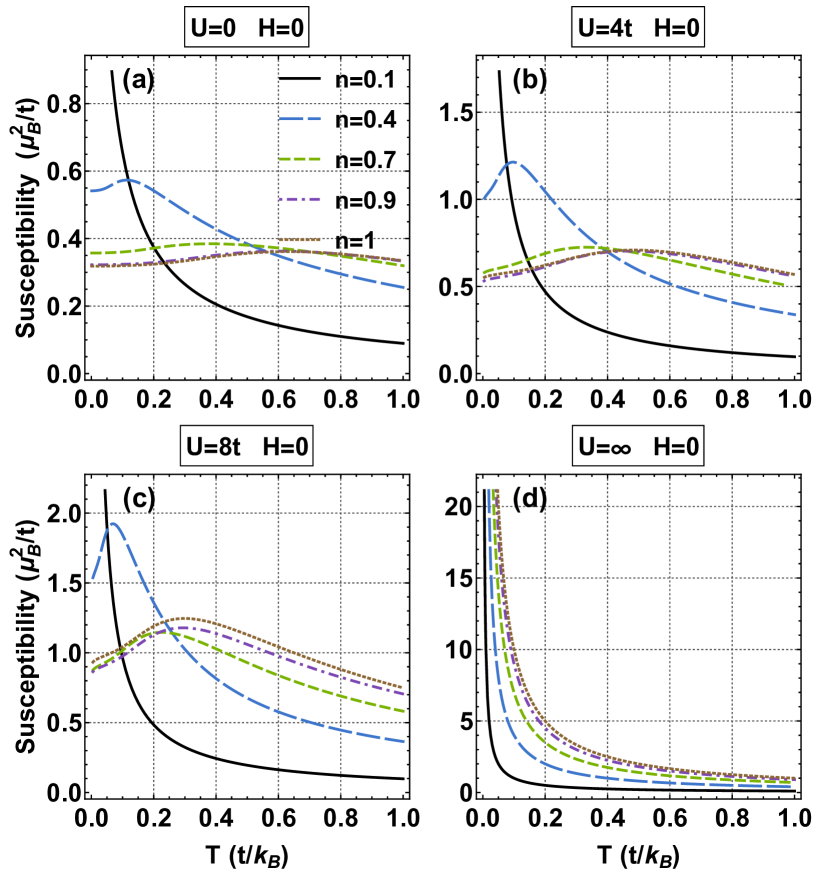
Figure 13: Temperature dependence of the susceptibility in zero magnetic field for various filling fractions and interaction strengths.

Figure 14: Temperature dependence of the susceptibility in the presence of a magnetic field. The values at $T=0$ denoted by squares $(H=0)$, disks $(H=0.1\,t/\mu_{B})$, triangles $(H=0.2\,t/\mu_{B})$ and diamonds $(H=0.3\,t/\mu_{B})$ are computed using Eqs. (17), (20) and given in Tables 3 and 4. The insets show the behavior at high temperatures.

At zero temperature and zero magnetic field the magnetic susceptibility was investigated in Tak3 ; Tak4 ; Shiba3 ; UF . The influence of a magnetic field was investigated in the very thorough article of Carmelo, Horsch and Ovchinnikov CHO and in KT1 . An interesting feature of the ground state susceptibility is that for all values of the filling fraction and on-site repulsion it presents a logarithmic dependence at low magnetic fields $(H\ll 1$) KT1 i.e.,

$$\chi(T=0)=\chi_{0}\left(1+\frac{1}{2\ln(a/H)}-\frac{\ln\ln(a/H)}{4(\ln(a/H))^{2}}\right)$$ (49)

where $a$ is a constant. At finite temperature numerical data for the magnetic susceptibility can be found in UKO2 ; KUO1 ; JKS ; Liu ; Ha . In KT1 (see also NBTVT ) the authors speculated that the susceptibility should also have a logarithmic dependence on temperature at any filling fraction and value of $U$, a conjecture which is confirmed by our numerical data.

In Fig. 13 we present the temperature dependence of the susceptibility in zero magnetic field for various filling fractions. For finite values of the interaction strength the behaviour is similar for all density values: the susceptibility is finite at $T=0$, presents a maximum which is inverse proportional with the filling fraction and whose position moves to higher temperatures as $n$ increases. At higher temperatures the susceptibility is an increasing function of the filling fraction. An interesting feature on which we will elaborate later is the presence of a logarithmic singularity at very low temperatures for $0<U<\infty$. The case of infinite repulsion is different. Here the magnetization is $m=n\tanh(H/T)/2$ and the susceptibility is infinite at $T=0$ for any value of $n$.

Figure 15: Logarithmic dependence of the susceptibility in zero magnetic field. The disks are numerical data and the lines represent best fits using Eq. (50).

Susceptibilities at $T=0$ and $U=4$
$\chi$	H=0	H=0.1	H=0.2	H=0.3
n=0.1	7.713 [IV]	0.515 [II]	0.515 [II]	0.515 [II]
n=0.4	0.926 [IV]	1.332 [IV]	2.561 [IV]	0.167 [II]
n=0.7	0.543 [IV]	0.639 [IV]	0.690 [IV]	0.764 [IV]
n=0.9	0.500 [IV]	0.577 [IV]	0.611 [IV]	0.656 [IV]

Table 3: Susceptibilities at zero temperature and $U=4$. The square parentheses identify the phase of the system. Note that we are dealing with the grand-canonical spin susceptibility which may be non-zero in the spin-polarized phase and independent of the field. In fact, this spin susceptibility $\chi$ is identical to the compressibility $\kappa$ see e.g. table 5.

Susceptibilities at $T=0$ and $U=8$
$\chi$	H=0	H=0.1	H=0.2	H=0.3
n=0.1	13.92 [IV]	0.515 [II]	0.515 [II]	0.515 [II]
n=0.4	1.403 [IV]	3.123 [IV]	0.167 [II]	0.167 [II]
n=0.7	0.816 [IV]	1.041 [IV]	1.280 [IV]	1.897 [IV]
n=0.9	0.807 [IV]	0.999 [IV]	1.168 [IV]	1.502 [IV]

Table 4: Susceptibilities at zero temperature and $U=8$. The square parentheses identify the phase of the system.

The influence of a magnetic field on the temperature dependence of the susceptibility is presented in Fig. 14. The general structure is the same as in the case of zero magnetic field: a finite value at $T=0$ followed by a maximum at low temperatures. As long as the magnetic field is not strong enough to fully polarize the system in the ground state the susceptibility increases with $H$ at low temperatures and the position of the maximum moves to higher temperatures as the magnetic field decreases (see panels (c), (d), (g) and (h) of Fig. 14). When the magnetic field polarizes the system the susceptibility is strongly suppressed and becomes a monotonically decreasing function of $H$ at low temperatures (see panels (a), (b), (e) and (f) of Fig. 14).

In both cases at higher temperatures the susceptibility is largest at $H=0$. The most interesting feature is the logarithmic singularity at low temperatures in zero magnetic field as it can be seen in Fig. 15 where we present our numerical results together with the fits using

$$\chi(T)=\chi(T=0)+\frac{a}{\ln(T_{0}/T)}\,.$$ (50)

where $a$ and $T_{0}$ are free parameters. At quarter filling an infinite slope of the susceptibility was obtained from renormalization group calculations NBTVT . The same logarithmic dependence was discovered in the case of the susceptibility of the XXX spin chain in EAT ; K3 . While one can say that this phenomenon can be intuitively inferred at half filling and large values of $U$ due to the equivalence of the spin sector with the XXX spin chain the logarithmic dependence at below half filling which can be seen in the numerical data even at $n=0.1$ and $U=4$ is intriguing.

VI.3 Compressibility

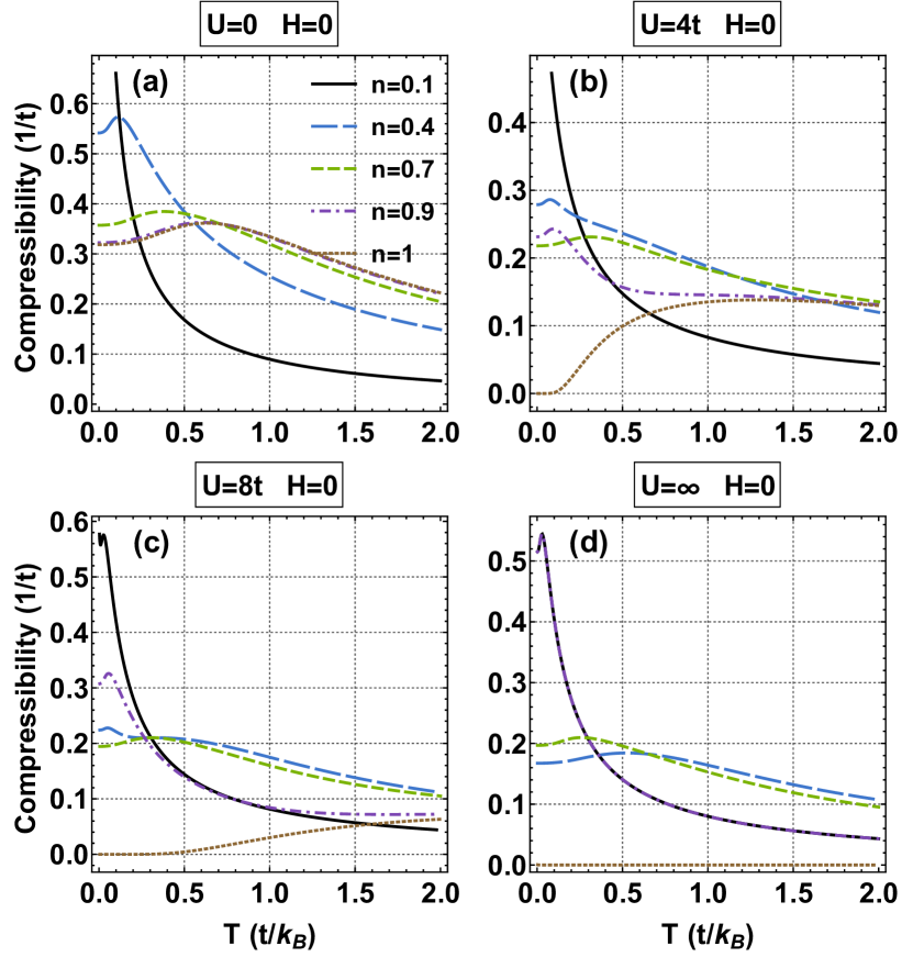
Figure 16: Temperature dependence of the compressibility in zero magnetic field for various filling fractions and interaction strengths.

Figure 17: Temperature dependence of the compressibility in the presence of a magnetic field. The values at $T=0$ denoted by squares $(H=0)$, disks $(H=0.1\,t/\mu_{B})$, triangles $(H=0.2\,t/\mu_{B})$ and diamonds $(H=0.3\,t/\mu_{B})$ are computed using Eqs. (17), (21) and given in Tables 5 and 6. The insets show the behavior at high temperatures.

The compressibility was investigated analytically and numerically at zero temperature in CHO and at finite temperature in UKO2 ; KUO1 ; JKS ; Ha . The temperature dependence of the compressibility in zero magnetic field and various densities and interaction strengths can be found in Fig. 16. For $0<U<\infty$ and $n=1$ (half filling) the charge sector has a gap resulting in zero compressibility at $T=0$ and exponentially activated behavior at low temperatures. At arbitrary filling fractions $\kappa$ is nonzero and in general presents only one maximum. However at very low fillings the compressibility is strongly enhanced and it can present two maxima at very low temperatures. Similar to the case of the specific heat at $U=\infty$ the compressibility satisfies $\kappa(n)=\kappa(1-n)$ for $n\in[0,1)$ (the curves for $n=0.1$ and $n=0.9$ coincide as in Fig. 11).

The influence of the magnetic field on compressibility is shown in Fig. 17. The presence of a magnetic field which polarizes the system at $n=0.1$ depresses the compressibility below the zero field value. In addition $\kappa$ presents only one maximum. Magnetic fields below the critical value in general enhance the compressibility and move the maximum to lower temperatures. For densities close to $n\sim 0.5$ large values of $H$ seem to develop a second maximum at low temperatures similar to the case of low fillings but a similar phenomenon was reported also for zero magnetic field in JKS .

Compressibilities at $T=0$ and $U=4$
$\kappa$	H=0	H=0.1	H=0.2	H=0.3
n=0.1	0.662 [IV]	0.515 [II]	0.515 [II]	0.515 [II]
n=0.4	0.278 [IV]	0.291 [IV]	0.403 [IV]	0.167 [II]
n=0.7	0.217 [IV]	0.218 [IV]	0.221 [IV]	0.227 [IV]
n=0.9	0.231 [IV]	0.232 [IV]	0.234 [IV]	0.240 [IV]

Table 5: Compressibilities at zero temperature and $U=4$. The square parentheses identify the phase of the system.

Compressibilities at $T=0$ and $U=8$
$\kappa$	H=0	H=0.1	H=0.2	H=0.3
n=0.1	0.587 [IV]	0.515 [II]	0.515 [II]	0.515 [II]
n=0.4	0.223 [IV]	0.250 [IV]	0.167 [II]	0.167 [II]
n=0.7	0.194 [IV]	0.195 [IV]	0.201 [IV]	0.217 [IV]
n=0.9	0.307 [IV]	0.309 [IV]	0.319 [IV]	0.339 [IV]

Table 6: Compressibilities at zero temperature and $U=8$. The square parentheses identify the phase of the system.

VII Thermodynamic properties at half filling

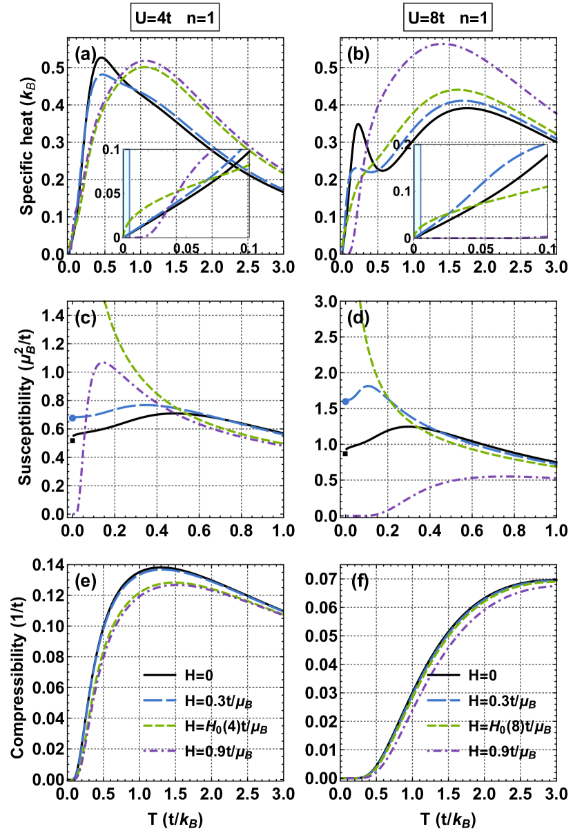
Figure 18: Temperature dependence of the specific heat, susceptibility and compressibility at half filling in the presence of a magnetic field. The insets present a zoom of the specific heat data at low temperatures. The shaded regions are inaccessible numerically and contain the theoretical predictions $c_{V}^{(c)}\sim\gamma T$ for $H<H_{0}(U),$ $c_{V}^{(c)}\sim aT^{1/2}$ for $H=H_{0}(U)\,t/\mu_{B}$ and $c_{V}^{(c)}\sim T^{3/2}e^{-\alpha/T}$ for $H=0.9\,t/\mu_{B}.$ The susceptibilities at $T=0$ denoted by squares $(H=0)$ and disks $(H=0.3\,t/\mu_{B})$ are computed using Eq. (22).

Historically the half filling case constitutes one of the most investigated regimes of the Hubbard model starting with the initial paper of Lieb and Wu LW . At half filling the charge sector has a gap and therefore the low temperature thermodynamics is influenced only by the spin excitations. At zero magnetic field and temperature the dressed charge for the half filled band is $\xi(A=\infty)=1/\sqrt{2}$ WE1 resulting in a specific heat coefficient and susceptibility (the compressibility is zero as a consequence of the charge gap)

$$\gamma_{\mbox{\tiny{HF}}}(H=0)=\frac{\pi}{3}\frac{1}{v_{s}}\,,\ \ \ \chi_{\mbox{\tiny{HF}}}(H=0)=\frac{4}{2\pi v_{s}}\,,$$ (51)

with the spin velocity

$$v_{s}=2I_{1}\left(\frac{\pi}{2u}\right)/I_{0}\left(\frac{\pi}{2u}\right)\,,$$ (52)

where $I_{n}(z)$ is the modified Bessel function of the first kind which for integer $n$ has the integral representation $I_{n}(z)=\frac{1}{\pi}\int_{0}^{\pi}e^{z\cos\theta}\cos(n\theta)\,d\theta\,.$ For magnetic fields $H<H_{0}(U)$ the system is partially polarized (phase V) and for $H>H_{0}(U)$ is fully polarized (phase III).

In Fig. 18 (a) and (b) we present the temperature dependence of the specific heat for $U=4$ and $U=8$ and several values of the magnetic $H=\{0,0.3\}<H_{0}(U),$ $H=H_{0}(U)$ and $H=0.9>H_{0}(U)$. At low and moderate interaction strengths and magnetic field below $H<H_{0}(U)$ the specific heat is linear in temperature $(\gamma(U=4,H=0)=0.853\,,\gamma(U=4,H=0.3)=0.933)$ and presents a single maximum which decreases with the increase of $H$. The results for $U=8$ show the double peak structure with the second maximum being proportional to the magnetic field ($(\gamma(U=8,H=0)=1.433\,,\gamma(U=8,H=0.3)=1.928)$. The specific heat coefficients monotonically increase as $H$ approaches $H_{0}(U)$ (the spin velocity decreases) the value for which they become infinite signalling the QPT from phase V to phase III. At the critical field the specific heat behaves like $c_{V}^{(c)}\sim a(U)\,T^{1/2}$ with $a(U=4)=0.261$ and $a(U=8)=0.332$ and presents only one maximum. For $H=0.9>H_{0}(U)$ the system presents thermally activated specific heat $c_{V}^{(c)}\sim T^{3/2}e^{-\alpha/T}$.

Results for the susceptibility are shown in Fig. 18 (c) and (d). For $H=0$ and $H=0.3$ the curves present only one maximum which moves to lower temperatures with increasing magnetic field and the zero field susceptibility presents logarithmic behaviour for low temperatures (see Fig. 15). For $T=0$ and magnetic fields lower than but close to $H_{0}(U)$ the susceptibility diverges like $1/(H_{0}-H)^{1/2}$ and for $H>H_{0}(U)$ vanishes. As a function of the temperature $\chi$ is divergent at low-$T$ and $H=H_{0}(U)$ and behaves like $e^{-\beta/T}$ for $H>H_{0}(U)$.

At half filling and zero temperature the compressibility is zero for all values of the magnetic field. At low temperatures it behaves like $e^{-\beta/T}$ and presents a single maximum which moves to higher temperatures as $U$ is increased (Fig. 18 (e) and (f)). At half filling the compressibility is a decreasing function of the magnetic field for all temperatures.

VIII Double occupancy

Figure 19: Double occupancy as a function of the density for different values of temperature, magnetic fields and $U=\{4t,8t\}.$ The insets contain the results for the density in the $(1,2]$ interval.

The computation of the correlation functions in the Hubbard model is an extremely difficult task even though in principle the wave functions and energy levels are known. However, one particular correlation function, which is also experimentally accessible, the double occupancy, can be determined from the thermodynamics of the system in a manner similar with the derivation of the contact in the case of continuous short range interaction models Tan1 ; Tan2 ; Tan3 ; OD ; BP1 ; ZL ; WC1 ; WC2 ; VZM1 ; VZM2 ; BZ ; PK2 . The double occupancy at site $j$ defined by $\langle n_{j,\uparrow}n_{j,\downarrow}\rangle$ quantifies the probability that a lattice site has two electrons. Due to translation invariance we have $\langle n_{j,\uparrow}n_{j,\downarrow}\rangle=\langle n_{k,\uparrow}n_{k,\downarrow}\rangle$ for any $j,k\in\{1,\cdots,L\}$ and we define $\langle n_{\uparrow}n_{\downarrow}\rangle=\sum_{j=1}^{L}\langle n_{j,\uparrow}n_{j,\downarrow}\rangle/L$. Using the definition of the grand canonical potential $\phi=-\ln Z/(\beta L)$ with $Z=\mbox{Tr}\left[e^{-\beta\mathcal{H}-\mu N-2Hm}\right]$ and the Helmann-Feynman theorem we find $\left(\frac{\partial\phi}{\partial U}\right)_{\mu,H,T}=\mbox{Tr}\left[\sum_{j=1}^{L}\left(n_{j,\uparrow}-\scalebox{0.8}{$\frac{1}{2}$}\right)\left(n_{j,\downarrow}-\scalebox{0.8}{$\frac{1}{2}$}\right)e^{-\beta\mathcal{H}-\mu N-2Hm}\right]/(LZ)$ and therefore

$$\langle n_{\uparrow}n_{\downarrow}\rangle=\left(\frac{\partial\phi}{\partial U}\right)_{\mu,H,T}+\frac{n}{2}-\frac{1}{4}\,.$$ (53)

At half filling the double occupancy was investigated in Shiba1 ; Shiba2 ; GKS ; GRPSK ; CCHQS ; STUBG and for the spin-disordered regime in EEG . The dependence on the temperature at any filling and zero magnetic field was studied by Campo Campo using the QTM equations.

Figure 20: Double occupancy at half filling as a function of the temperature for different values of $U$ and magnetic fields $H=\{0,0.15\,t/\mu_{B},0.3\,t/\mu_{B}\}.$ The double occupancy presents two minima for intermediate values of $U$ (a) and for large values of $U$ and magnetic field close to the critical value (d) ($H_{0}(12)\sim 0.3245\,t/\mu_{B}$).

The double occupancy $d(n)$ takes values between 0 and 1 and unlike many other thermodynamic functions it is not symmetric with respect to $n=1$. From (45) we find by differentiation with respect to $u$ the relation $d(n)=d(2-n)+n-1$. At zero temperature it is a continuous function of $n\in[0,2]$ but the derivative is discontinuous at half filling. Numerical results for different temperatures and magnetic fields are presented in Fig. 19. For free particles on the lattice one would expect that $\langle n_{\uparrow}n_{\downarrow}\rangle$ would monotonically increase with temperature. In the Hubbard model due to the repulsive interaction term this simple picture does not hold. At zero magnetic field and $U=4$ (panel (a) of Fig. 19) the free particle picture holds for small filling fractions where the interaction is not that important. For $n\sim 0.3$ a crossover appears and the double occupancy for $T=0.1$ is larger than the equivalent quantity at $T=0.5$ for $n\in(0.3,1)$. Switching a magnetic field (panel (b) of Fig. 19) moves the crossover density closer to half filling. At fixed temperature the magnetic field suppresses the double occupancy as it can be seen in Fig. 19 (c) and (d). This is due to the fact that the magnetic field polarizes the system and therefore the probability to have two electrons is doubly penalized by the Pauli principle and the repulsive interaction. Also at fixed temperature $\langle n_{\uparrow}n_{\downarrow}\rangle$ is a monotonically decreasing function of interaction strength and magnetic field as the system becomes more easily polarizable as $U$ increases.

At half filling and zero temperature and magnetic field the double occupancy can be obtained in analytic form from the ground state energy of Lieb and Wu

$$\langle n_{\uparrow}n_{\downarrow}\rangle_{0}(U)=\frac{1}{2}\int_{0}^{\infty}d\omega J_{0}(\omega)J_{1}(\omega)\mbox{sech}^{2}(\omega U/4)\,,$$ (54)

with $J_{n}(\omega)=\frac{1}{\pi}\int_{0}^{\pi}\cos(\omega\sin\theta-n\theta)\,d\theta$ the $n$th Bessel function of the first kind. At low temperatures $(T\ll t)$ we have CCHQS ; KBar

$$\langle n_{\uparrow}n_{\downarrow}\rangle(T)\underset{T\ll t}{\simeq}\langle n_{\uparrow}n_{\downarrow}\rangle_{0}(U)-\frac{1}{2}\mathcal{C}(2\pi/U)T^{2}+O(T^{3})$$ (55)

with

$$\mathcal{C}(x)=\frac{x^{2}}{12}\left(1-\frac{I_{0}(x)[I_{0}(x)+I_{2}(x)]}{I_{1}(x)^{2}}\right)$$ (56)

and at high temperatures $(T>t^{2}/U)$ the following expansion is valid CCHQS ; TS

$$\langle n_{\uparrow}n_{\downarrow}\rangle(T) \underset{T>t^{2}/U}{\simeq}-\frac{1}{2}\left(-TU+TU\cosh(U/2T)\right)^{-1}$$

$$+\tanh(U/4T)\mbox{sech}^{2}(U/4T)/(8T^{2})$$

$$+\frac{1}{2}\frac{1-4U^{-2}}{e^{U/2T}+1}+1/U^{2}+O(T^{-4})\,.$$ (57)

At half filling the dependence of the double occupancy on the temperature in the presence of a magnetic field for $U=\{3,4,8,12\}$ is shown in Fig. 20. At low temperatures and for all values of the coupling strength the double occupancy decreases with increasing temperature. This is relatively counterintuitive but it facilitates spin excitations which are entropically preferred (also notice that at zero magnetic field the function $\mathcal{C}(x)$ is positive for all $U$ CCHQS ). It is easy to see from (53) and the definition of the entropy that at half filling these quantities satisfy the Maxwell relation $\partial s/\partial U=-\partial\langle n_{\uparrow}n_{\downarrow}\rangle/\partial T$ which shows that the decrease of the double occupancy is accompanied by an increase of the entropy which is an analog of the Pomeranchuk effect Pomer ; Rich . For large values of the on-site repulsion ($U\geq 4$) and moderate magnetic fields the double occupancy presents only one minimum which moves to lower temperatures with increasing $H$. At intermediate values of $U$ it can be seen in Fig. (20)(a) that $\langle n_{\uparrow}n_{\downarrow}\rangle$ presents a two minima phenomenon which was first reported in STUBG in the case of zero magnetic field. Here we show that a similar doubly nonmonotonic (two local minima) behavior is present at large interaction strengths and magnetic fields close to the critical value $H_{0}(U)$ (see Fig. 20 (d)). Also in this case the specific heat presents three maxima instead of two as in the case of zero or moderate magnetic field. For all values of the interaction strength and half filling the double occupancy is a monotonically decreasing function of the magnetic field.

Figure 21: (a), (b), (e), (f): Dependence of the entropy on the density for different temperatures and magnetic fields. (c), (d), (g), (h): Dependence of the ratio of the entropy of the Hubbard model to the entropy of lattice free fermions on the filling factor.

IX Entropy

In the left panels of Fig. 21 we present the dependence of the entropy $s=-\left(\frac{\partial\phi}{\partial T}\right)_{\mu,H}$ on the density for different temperatures and magnetic fields. Similar results at zero magnetic field were reported in Campo . The right panels contain the ratios between the entropy of the Hubbard model and that of a system of free fermions at the same density. The dependence of the entropy on the filling factor is highly nonmonotonic at low temperatures. For $U=4$ and zero magnetic field the $T=0.1$ curve presents two local maxima in the $[0,1]$ interval and minima at endpoints (the entropy is symmetric in $n$ with respect to $n=1$). Increasing the temperature the dependence becomes smoother with the well known high temperature enveloping curve

$$s(T\gg 1)=2\ln\left(\frac{2}{2-n}\right)-n\ln\left(\frac{n}{2-n}\right)\,.$$ (58)

The origin of the two maxima is due to the quantum phase transitions, phase I to phase IV, for the first maximum and phase IV to phase V for the second one. In the presence of a magnetic field the entropy presents three maxima at low temperatures as a consequence of the three QPTs (phase I to phase II, phase II to phase IV and phase IV to phase V) present in the phase diagram for $H<H_{0}(U)$. For a fixed temperature the magnetic field decreases the entropy at low fillings compared with the $H=0$ case and close to half filling the effect is inverse (see Fig. 21 panels (e) and (f)). It should be noted that for $U=8$, $H=0.5$ is larger than $H_{0}(8)$ and therefore the entropy presents only two maxima as the system has only two QPTs (phase I to phase II and phase II to phase III).

The ratio $s/s_{FF}$ with $s_{FF}$ the entropy of a system of lattice free fermions at the same density measures the deviations from the free system. We see in Fig. 21 (c), (d), (g) and (h) that this ratio presents large deviations from 1 as we increase the interaction strength (as expected) but also as we increase the magnetic field as long as $H<H_{0}(U)$.

X Density profiles

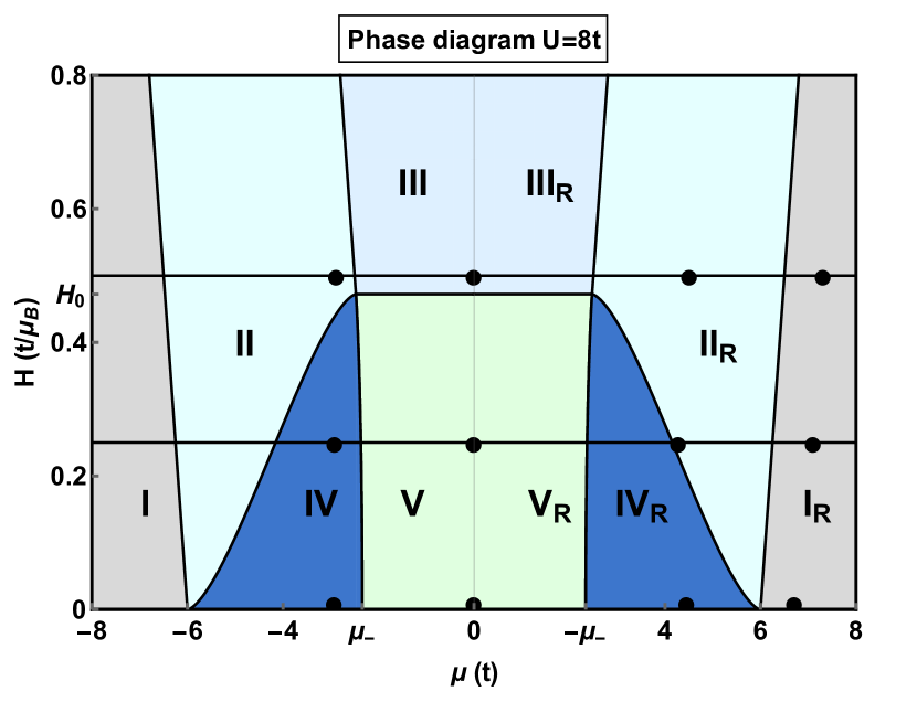
Figure 22: Phase diagram at zero temperature for $U=8$ and both positive and negative values of the chemical potential. The three horizontal lines pass through $H=\{0,0.25\,t/\mu_{B},0.5\,t/\mu_{B}\}$ and the disks on each one correspond to values of the chemical potential for which the density is (from left to right) $n=\{0.8,1,1.5,2\}$.

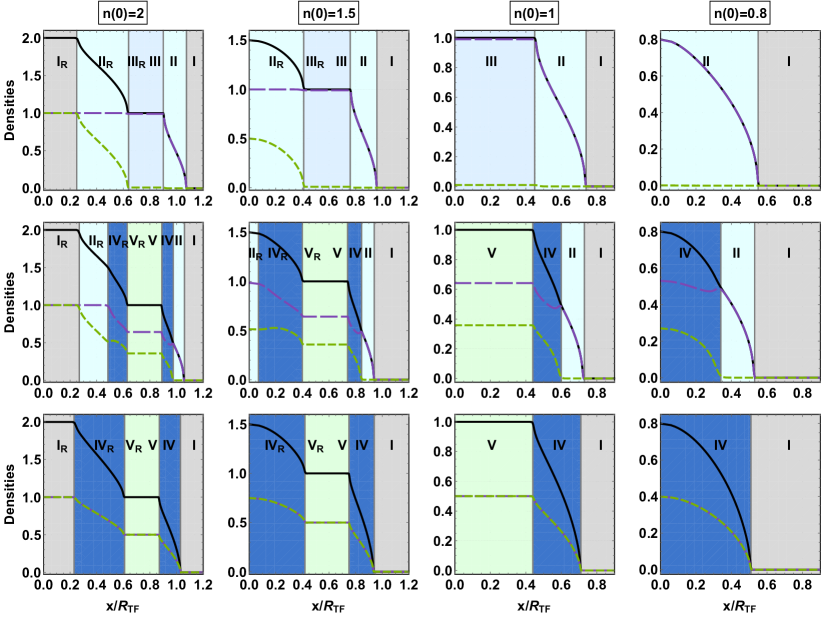
Figure 23: Density profiles for the Hubbard model in the presence of a trapping potential at $T=0.025t$, $U=8t$ and $H=0.5\,t/\mu_{B}$ (top row), $H=0.25\,t/\mu_{B}$ (middle row) and $H=0$ (bottom row). The profiles are symmetric with respect to $x$. Here we present only the $x>0$ region. At this temperature the density profiles are effectively indistinguishable from the ones at $T=0$. The black, violet and green lines represent the total density $n(x)=n_{\uparrow}(x)+n_{\downarrow}(x)$, the density of spin up electrons $n_{\uparrow}(x)$ and the density of spin down electrons $n_{\downarrow}(x)$. Each phase of the system is highlighted in the same color as in the phase diagram presented in Fig. 22.

The experimental realization of various physical models of interest using ultracold atoms in optical lattices require a trapping potential. In the case of the Hubbard model the presence of a harmonic trap is equivalent with the addition to the Hamiltonian (1) of a site dependent potential of the type

$$\mathcal{H}_{trap}=\sum_{j,\sigma}\frac{m\omega_{e}^{2}}{2}j^{2}n_{j\sigma}\,,$$ (59)

with $\omega_{e}$ the effective trap frequency. The addition of such a term breaks the integrability of the Hubbard model but considering a large system and a slowly varying trapping potential the thermodynamic properties of the inhomogeneous system can be computed using the homogeneous solution and the Local Density Approximation (LDA) LDH . Replacing the site index $j$ with a dimensionless variable $x$ the LDA assumes that each region at distance $x$ from the center of the trap can be well approximated by a homogeneous system with

$$\mu(x)=\mu(0)-\frac{m\omega_{e}^{2}}{2}x^{2}\,,\ \ \ H(x)=H(0)\,,$$ (60)

where $\mu(0)$ and $H(0)$ are the values of the chemical potential and magnetic field at the center of the trap. For given values of $\mu(0),H(0)$ (or equivalently $n(0)$ and $H$ with $n(0)$ the density at the center of the trap) the density profiles can be computed using the QTM equations (24) and (60). Density profiles for the balanced system were previously investigated using quantum Monte Carlo simulations RMBS , density functional theory XPTCC ; Campo and DMRG FHM ; HOF .

We are going to investigate density profiles with $0<n(0)\leq 2$ in the presence of a magnetic field. The phase diagram at zero temperature for both negative and positive values of the chemical potential (corresponding to $n\in[0,2]$) is shown in Fig. 22. The properties of the phases at $\mu>0$ which are in one-to-one correspondence with the five regimes analyzed in Sect. III.1 can be determined using the symmetry relation (45) and Eqs. (46). For given values of $U$, $m$ and $\omega_{e}$ we introduce a radius denoted by $R_{TF}$ and defined by

$$2\mu_{0}-\frac{m\omega_{e}^{2}}{2}R_{TF}^{2}=0\,,$$ (61)

with $\mu_{0}=2(U/4)+2$ the value of the chemical potential for which the density in the center of the trap is $n(0)=2$ at zero temperature and magnetic field. $R_{TF}$ is the distance from the center of the trap at which the density profile is zero for a system in the ground state with $n(0)=2$ and $H=0$.

In Fig. 23 we present the density profiles for a system with interaction strength $U=8$, $T=0.025$ and three values of the magnetic field $H=\{0,0.25,0.5\}$ where $H=0.5>H_{0}(8)$. The temperature chosen is so low that our results are almost indistinguishable from the $T=0$ case. The structure of the density profiles is intricate, especially for $n(0)>1$, but it can be easily understood by looking at the phase diagram from Fig. 22. Consider the case of $n(0)=2$ and $H=0.5$. Moving further from the center of the trap (increasing $x$) is equivalent with the chemical potential moving in the phase diagram from right to left along a horizontal line (in this case the starting value of $\mu$ is the rightmost point on the $H=0.5$ line of Fig. 22). As $x$ increases from zero the system crosses the following phases in order: $\mbox{I}_{R}$, $\mbox{II}_{R}$, $\mbox{III}_{R}$, III, II and finally I. The total density profile can be described as a band insulator at the trap center surrounded by metallic regions in turn surrounded by Mott insulators LDH . For $n(0)=2$ and $H=0.25$ (the starting value of the chemical potential is the rightmost point on the $H=0.25$ line) the system crosses the phases: $\mbox{I}_{R}$, $\mbox{II}_{R}$, $\mbox{IV}_{R}$, $\mbox{V}_{R}$, V, IV, II and I. While the total density profile is similar with the previous case (the metallic regions present angular points at the $\mbox{II}_{R}\rightarrow\mbox{IV}_{R}$ and IV $\rightarrow$ II transitions) the spin up and spin down density profiles are very different as $H=0.5$ is larger than the critical field while $H=0.25$ is below $H_{0}(8)$. Zero magnetic field is characterized by $n_{\uparrow}(x)=n_{\downarrow}(x)=n(x)/2$ and it comprises the following phases $\mbox{I}_{R}$, $\mbox{IV}_{R}$, $\mbox{V}_{R}$, V, IV, and I. The profiles with $n(0)<2$ can be understood in the same way and noticing that in this case the starting point of the chemical potential moves to the left which means that the system can skip some of the phases enumerated in the $n(0)=2$ case. At $n(0)=1.5$ the total density profiles can be characterized by a metallic center surrounded by Mott insulator plateaus while for $n(0)=1$ we encounter the situation of a Mott insulator at the center surrounded by metallic wings. Finally, for $n(0)=0.8$ the system is completely metallic. In all cases the structure of the total density profile is similar for the same value of the density at the center of the trap but the density profiles of the components are heavily influenced by the presence of the magnetic field.

XI Conclusions

In this paper we have studied the influence of the magnetic field on the quantum critical behavior and thermodynamic properties of the 1D repulsive Hubbard model. Even though all the QPTs investigated were characterized by critical exponents $z=2$ and $\nu=1/2$ the universal thermodynamics in the vicinity of the QCPs is not described by free fermions in all cases. The transitions from the vacuum belong to the universality class of spin-degenerate impenetrable particle gas and the universal thermodynamics is given by Takahashi’s formula. The influence of the magnetic field on the thermodynamic properties is very important at low temperature and small filling fractions. The magnetic susceptibility at zero magnetic field presents an infinite slope at low temperatures for all values of the filling fractions. The double occupancy exhibits two minima as a function of temperature in two situations: a) at intermediate values of $U$ and b) for large values of the repulsion and magnetic fields close to the critical value. In all the other cases the double occupancy presents only one minimum. In the experimentally relevant case of a trapped system the magnetic field does not influence strongly the overall density profiles but changes dramatically the distribution of phases in the inhomogeneous system. An interesting extension of our work is the case of the Hubbard model with impurities. This will be addressed in a future publication.

Appendix A Numerical implementation of the first type of convolutions

From the numerical point of view the main difficulty in the implementation of the QTM integral equations (24) is the treatment of the convolutions. The first type of convolutions is defined by

$$K*f=\int_{-\infty}^{+\infty}K(x-y)f(y)\,dy\,,$$ (62)

where the kernels (defined in (25)) can be $K_{2,\pm\alpha-\alpha}(x)\,,K_{1,\pm\alpha}(x)$ or $\overline{K}_{1,\pm\alpha}(x)$ with $0<|\alpha|<u\,$ and $f_{\alpha}(x)=f(x+i\alpha).$ The integrands are $\ln(1+\mathfrak{b}^{\pm}(x))$ or $\ln(1+1/\mathfrak{b}^{\pm}(x)).$ In general the most efficient way of treating convolutions is using the Fast Fourier Transform (FFT). However, in order to obtain accurate results FFT requires that the functions are either periodic or they decrease rather fast at infinity. In our case the kernels are relatively slowly decaying while the $\mathfrak{b}^{\pm}(x)$ functions have constant asymptotics at infinity, $\lim_{x\rightarrow\pm\infty}\ln\mathfrak{b}^{\pm}(x)=-\beta H$. Denoting by $f(\infty)=\lim_{x\rightarrow\pm\infty}f(x)$ the efficient way of treating this type of convolutions is by subtracting the asymptotic value

$$\int_{-\infty}^{+\infty}K(x-y) f(y)\,dy=\int_{-\infty}^{+\infty}K(x-y)[f(y)-f(\infty)]\,dy$$

$$+f(\infty)\int_{-\infty}^{+\infty}K(x-y)\,dy\,.$$ (63)

In the first term on the right hand side now both the kernel and the integrand vanish at infinity and can be calculated using FFT and an appropriate cutoff while the second term can be analytically computed. We find

$$\int_{-\infty}^{+\infty}K_{2,0}(x-y)\,dy =1\,,$$ (64a)

$$\int_{-\infty}^{+\infty}K_{2,2\alpha}(x-y)\,dy =1\,,$$ (64b)

$$\int_{-\infty}^{+\infty}K_{1,\alpha}(x-y)\,dy =0\,,$$ (64c)

$$\int_{-\infty}^{+\infty}K_{1,-\alpha}(x-y)\,dy =1\,,$$ (64d)

$$\int_{-\infty}^{+\infty}\overline{K}_{1,\alpha}(x-y)\,dy =1\,,$$ (64e)

$$\int_{-\infty}^{+\infty}\overline{K}_{1,-\alpha}(x-y)\,dy =0\,.$$ (64f)

Let us show how to compute these integrals. It is sufficient to consider the case of

$$I_{1}=\int_{-\infty}^{+\infty}K_{1,\alpha}(x-y)\,dy$$

all the other cases being amenable to a similar derivation. Making the change of variables $x-y=z$ we obtain

$$I_{1}=\int_{-\infty}^{+\infty}\frac{u/\pi}{(z+i\alpha)(z+i\alpha+2iu)}\,dz\,.$$

First, we will consider the case of $\alpha>0$. The integrand has two poles in the complex plane situated at $z_{1}=-i\alpha$ and $z_{2}=-i\alpha-2iu$. Closing the contour in the upper half plane by adding an infinite semicircle (which does not give a contribution) the integral is analytic inside the closed contour and we obtain $I_{1}=0$ proving (64c). In the case of $\alpha<0$ again closing the contour in the upper half plane we obtain $I_{1}=2\pi i\,\mbox{Res}(z=i|\alpha|)$ which gives $I_{1}=1$ proving (64d). All the other integrals can be computed in a similar fashion.

Appendix B Numerical implementation of the second type of convolutions

The numerical implementation of the second type of convolutions defined by

$$K\bullet f=\mbox{p.v.}\int_{-1}^{+1}K(x-y)f(y)\,dy\,,$$

is more complicated due to the presence of the principal value integral and also because the integrands $\ln(1+\mathfrak{c}^{\pm}(x))$ and $\ln(1+\overline{\mathfrak{c}}^{\pm}(x))$ behave like $(1-x^{2})^{1/2}$ in the vicinity of $\pm 1$. This weakly singular behavior suggest that the best way to tackle these convolutions numerically is to employ Chebyshev quadratures. First we will present some minimal information on Chebyshev polynomials necessary to derive relevant quadrature formulae.

B.1 Chebyshev polynomials

We are going to use only Chebyshev polynomials of the first and second type defined by MH

$$T_{n}(x) =\cos n\theta\,,\ x=\cos\theta\,,\ \ \theta\in[0,\pi]\,,$$ (65)

$$U_{n}(x) =\frac{\sin[(n+1)\theta]}{\sin\theta}\,,\ x=\cos\theta\,,\ \ \theta\in[0,\pi]\,.$$ (66)

The zeroes of $T_{n}(x)$ and $U_{n}(x)$ are given by

$$T_{n}(x): \ x_{k}=\cos\left[\frac{(k-1/2)\pi}{n}\right]\,, \ \ k =1,\ldots,n\,,$$

$$U_{n}(x): \ y_{k}=\cos\left[\frac{k\pi}{n+1}\right]\,, \ \ k =1,\ldots,n\,\,.$$

In the $z=\cos\theta$ variable the Chebyshev polynomials take the form

$$T_{n}(x) =\frac{1}{2}\left[(z+\sqrt{z^{2}-1})^{n}+(z-\sqrt{z^{2}-1})^{n}\right]\,,$$ (67)

$$U_{n}(x) =\frac{1}{2}\frac{(z+\sqrt{z^{2}-1})^{n}+(z-\sqrt{z^{2}-1})^{n}}{\sqrt{z^{2}-1}}\,.$$ (68)

B.2 Chebyshev-Gauss quadrature

In this section we remind the reader of the derivation of the Chebyshev-Gauss quadrature of the second kind which will constitute the basis for a similar result for principal value integrals. We want to obtain a quadrature for the integral

$$I(f)=\int_{-1}^{1}f(x)\,dx\,,$$ (69)

where $f(x)\sim(1-x^{2})^{1/2}$ at the endpoints of the interval but this requirement can be dropped. We approximate $f(x)$ by a function of the form

$$J_{n-1}[f(x)]=(1-x^{2})^{1/2}\sum_{j=0}^{n-1}b_{j}U_{j}(x)\,,$$ (70)

and we introduce

$$I_{n-1}(f)=\int_{-1}^{1}J_{n-1}[f(x)]\,dx\,,$$ (71)

which constitutes an approximation of the integral (69) using an interpolating polynomial of order $n-1$. Using the second kind discrete orthogonality formula (8.33 of MH )

$$d_{ij}=\sum_{k=1}^{n}(1-y_{k}^{2})U_{i}(y_{k})U_{j}(y_{k})=\left\{\begin{array}[]{l}\frac{1}{2}(n+1)\,,\ i=j\leq n-1\,,\\ 0\,,i\neq j\end{array}\right.$$

with $y_{k}=\cos(k\pi/n+1)\,,k=1,\ldots,n$ the zeroes of the Chebyshev polynomials of the second type we obtain

$$b_{j}=\frac{2}{n+1}\sum_{k=1}^{n}(1-y_{k})^{1/2}f(y_{k})U_{j}(y_{k})\,.$$ (72)

Integrating (70) we find $I_{n-1}(f)=\sum_{j=0}^{n-1}b_{j}a_{j}$ with $a_{j}=\int_{-1}^{1}(1-x^{2})^{1/2}U_{j}(x)\,dx.$ The coefficients $a_{j}$ can be calculated analytically with the result

$$a_{j}=\int_{0}^{\pi}\sin[(j+1)\theta]\sin\theta\,d\theta=\left\{\begin{array}[]{l}\frac{\pi}{2}\,,j=0\,,\\ 0\,,j>0\,.\end{array}\right.$$

Collecting everything we find

$$\int_{-1}^{1}f(x)\,dx\sim I_{n-1}(f)=\sum_{k=1}^{n}\omega_{k}f(y_{k})\,,$$ (73)

with

$$\omega_{k} =\frac{\pi}{n+1}\sin\left[\frac{k\pi}{n+1}\right]\,, \ \ k =1,\ldots,n\,,$$ (74a)

$$y_{k} =\cos\left[\frac{k\pi}{n+1}\right]\,, \ \ k =1,\ldots,n\,.$$ (74b)

Formulae (73) and (74) represent the Chebyshev-Gauss quadrature of the second kind which are very efficient in the numerical integration of functions which behave like $(1-x^{2})^{1/2}$ at the endpoints of $[-1,1]$.

B.3 Chebyshev-Gauss quadrature for principal value integrals

The same method can be used to derive a quadrature formula for principal value integrals of the type

$$I_{\mathcal{C}}(f)=\mbox{p.v.}\int_{-1}^{1}\frac{f(x)}{y-x}\,dx\,,\ \ |y|<1\,.$$ (75)

Using the same approximation (70) for the $f(x)$ function and repeating verbatim the steps from the previous section we obtain $I_{\mathcal{C},n-1}(f)=\sum_{j=0}^{n-1}b_{j}a_{j}[y]$ with

$$a_{j}[y]=\mbox{p.v.}\int_{-1}^{1}(1-x^{2})^{1/2}\frac{U_{j}(x)}{y-x}\,dx=\pi T_{j+1}(y)\,,$$ (76)

where the final result was derived using Theorem 9.1 of MH . Together with (72) we find that $I_{\mathcal{C},n-1}(f)=\sum_{k=1}^{n}\omega_{k}(y)f(y_{k})$ with

$$\omega_{k}(y)=\sum_{j=0}^{n-1}\frac{2\pi T_{j+1}(y)}{n+1}\sin\left[\frac{k\pi}{n+1}\right]U_{j}\left[\cos\left(\frac{k\pi}{n+1}\right)\right]\,.$$

Using $\sin\left[\frac{k\pi}{n+1}\right]U_{j}\left[\cos\left(\frac{k\pi}{n+1}\right)\right]=\sin\left[\frac{(j+1)k\pi}{n+1}\right]$ we obtain the main result of this Appendix

$$\mbox{p.v.}\int_{-1}^{1}\frac{f(x)}{y-x}\,dx\,\sim I_{\mathcal{C},n-1}(f)=\sum_{k=1}^{n}\omega_{k}(y)f(y_{k})\,,$$ (77)

with

$$\omega_{k}(y) =\sum_{j=1}^{n}\frac{2\pi}{n+1}T_{j}(y)\sin\left[\frac{(j+1)k\pi}{n+1}\right]\,,$$ (78a)

$$y_{k} =\cos\left[\frac{k\pi}{n+1}\right]\,,\ \ \ \ k=1,\ldots,n\,.$$ (78b)

References

- (1) J. Hubbard, Electron correlations in narrow energy bands, Proc. R. Soc. (London) A 276, 238 (1963).
- (2) J. Hubbard, Electron correlations in narrow energy bands. 2. Degenerate band case, Proc. R. Soc. (London) A 277, 237 (1964).
- (3) M.C. Gutzwiller, Effect of correlation on ferromagnetism of transition metals, Phys. Rev. Lett. 10, 159 (1963).
- (4) J. Kanamori, Electron correlation and ferromagnetism of transition metals, Prog. Theor. Phys. 30, 275 (1963).
- (5) F.H.L. Essler, H. Frahm, F. Göhmann, A. Klümper, and V.E. Korepin, The One-Dimensional Hubbard Model (Cambridge University Press, Cambridge, England, 2005).
- (6) M.Boll, T.A. Hilker, G. Salomon, A. Omran, J. Nespolo, L. Pollet, I. Bloch, C. Gross, Spin- and density-resolved microscopy of antiferromagnetic correlations in Fermi-Hubbard chains, Science 353, 1257 (2016).
- (7) T.A. Hilker, G. Salomon, F. Grusdt, A. Omran, M. Boll, E. Demler, I.Bloch, C. Gross, Revealing Hidden Antiferromagnetic Correlations in Doped Hubbard Chains via String Correlators, Science 357, 484 (2017).
- (8) G. Salomon, J. Koepsell, J. Vijayan, T.A. Hilker, J. Nespolo, L. Pollet, I. Bloch, C. Gross, Direct observation of incommensurate magnetism in Hubbard chains, Nature 565, 56 (2019).
- (9) S. Scherg, T. Kohlert, J. Herbrych, J. Stolpp, P. Bordia, U. Schneider, F. Heidrich-Meisner, I. Bloch, and M. Aidelsburger, Nonequilibrium Mass Transport in the 1D Fermi-Hubbard Model, Phys. Rev. Lett. 121, 130402 (2018).
- (10) F.D.M. Haldane, ’Luttinger liquid theory’ of one-dimensional quantum fluids. I. Properties of the Luttinger model and their extension to the general 1D interacting spinless Fermi gas, J. Phys. C 14, 2585 (1981).
- (11) T. Giamarchi, Quantum Physics in One Dimension, (Oxford University Press, Oxford, England, 2003).
- (12) E.H. Lieb and F. Y. Wu, Absence of Mott Transition in an Exact Solution of the Short-Range, One-Band Model in One Dimension, Phys. Rev. Lett. 20, (1968); Erratum: Phys. Rev. Lett. 21, 192 (1968).
- (13) A.A. Ovchinnikov, Excitation spectrum of the one-dimensional Hubbard model, Sov. Phys. JETP 30, 1160 (1970).
- (14) G.V. Uimin and G.V. Fomichev, Excitations in the one-dimensional Hubbard model, Sov. Phys. JETP 36, 1001 (1973).
- (15) C.F. Coll, Excitation spectrum of the one-dimensional Hubbard model, Phys. Rev. B 9, 2150 (1974).
- (16) F. Woynarovich, Excitations with complex wavenumbers in a Hubbard chain: I. States with one pair of complex wavenumbers, J. Phys. C 15, 85 (1982).
- (17) F. Woynarovich, Excitations with complex wavenumbers in a Hubbard chain: II. States with several pairs of complex wavenumbers, J. Phys. C 15, 97 (1982).
- (18) F. Woynarovich, Spin excitations in a Hubbard chain, J. Phys. C 16, 5293 (1983).
- (19) A. Klümper, A. Schadschneider, and J. Zittartz, A new method for the excitations of the one-dimensional Hubbard model,Z. Phys. Con. Mat. 78, 99 (1990).
- (20) F.H.L. Essler and V.E. Korepin, Scattering matrix and excitation spectrum of the Hubbard model, Phys. Rev. Lett. 72, 908 (1994).
- (21) T. Deguchi, F.H.L. Essler, F. Göhmann, A. Klümper, V.E. Korepin, and K. Kusakabe, Thermodynamics and excitations of the one-dimensional Hubbard model, Phys. Rep. 331, 197 (2000).
- (22) F.H.L. Essler, V.E. Korepin, and K. Schoutens Complete solution of the one-dimensional Hubbard model, Phys. Rev. Lett. 67, 3848 (1991).
- (23) M. Takahashi, Magnetization Curve for the Half-Filled Hubbard Model, Prog. Theor. Phys. 42, 1098 (1969); Erratum: Prog. Theor. Phys. 43, 860 (1970).
- (24) M. Takahashi, Magnetic Susceptibility for the Half-Filled Hubbard Model, Prog. Theor. Phys. 43, 1619 (1970).
- (25) H. Shiba, Magnetic Susceptibility at Zero Temperature for the One-Dimensional Hubbard Model, Phys. Rev. B 6, 930 (1972).
- (26) J.M.P. Carmelo, P. Horsch, and A.A. Ovchinnikov, Static properties of one-dimensional generalized Landau liquids, Phys. Rev. B 45, 7899 (1992).
- (27) C.N. Yang, pairing and off-diagonal long-range order in a Hubbard model, Phys. Rev. Lett. 63, 2144 (1989).
- (28) D.B. Uglov and V.E. Korepin, The Yangian symmetry of the Hubbard model, Phys. Lett. A 190, 238 (1994).
- (29) S. Murakami and F. Göhmann, Yangian Symmetry and Quantum Inverse Scattering Method for the One-Dimensional Hubbard Model, Phys. Lett. A 227, 216 (1997).
- (30) S. Murakami, F. Göhmann, Algebraic Solution of the Hubbard Model on the Infinite Interval, Nucl. Phys. B 512, 637 (1998).
- (31) M. Ogata and H. Shiba, Bethe-ansatz wave function, momentum distribution, and spin correlation in the one-dimensional strongly correlated Hubbard model, Phys. Rev. B 41, 2326 (1990).
- (32) M. Ogata, T. Sugiyama, and H. Shiba, Magnetic-field effects on the correlation functions in the one-dimensional strongly correlated Hubbard model, Phys. Rev. B 43, 8401 (1991).
- (33) H.J. Schulz, Correlation exponents and the metal-insulator transition in the one-dimensional Hubbard model, Phys. Rev. Lett. 64, 2831 (1990).
- (34) H.J. Schulz, Correlated fermions in 1 dimension, Int. J. Mod. Phys. B 5, 57-74 (1991).
- (35) H. Frahm and V. E. Korepin, Critical exponents for the one-dimensional Hubbard model, Phys. Rev. B 42, 10553 (1990).
- (36) H. Frahm and V. E. Korepin, Correlation functions of the one-dimensional Hubbard model in a magnetic field, Phys. Rev. B 43, 5653 (1991).
- (37) A. Parola and S. Sorella, Asymptotic spin-spin correlations of the one-dimensional Hubbard model, Phys. Rev. Lett. 64, 1831 (1990).
- (38) A. Parola and S. Sorella, Spin-charge decoupling and the Green’s function of one-dimensional Mott insulators, Phys. Rev. B 45, 13156(R) (1992).
- (39) C.A. Stafford and A.J. Millis, Scaling theory of the Mott-Hubbard metal-insulator transition in one dimension, Phys. Rev. B 48, 1409 (1993).
- (40) Z. Y. Weng, D. N. Sheng, C. S. Ting, and Z. B. Su, Path-integral approach to the one-dimensional large-U Hubbard model, Phys. Rev. B 45, 7850 (1992).
- (41) Z. Y. Weng, Phase shift, the Marshall sign, and the Luttinger-liquid behavior in one dimension, Phys. Rev. B 50, 13837 (1994).
- (42) K. Penc, F. Mila, and H. Shiba, Spectral Function of the 1D Hubbard Model in the Limit, Phys. Rev. Lett. 75, 894 (1995).
- (43) K. Penc, K. Hallberg, F. Mila, and H. Shiba, Shadow Band in the One-Dimensional Infinite- Hubbard Model, Phys. Rev. Lett. 77, 1390 (1996).
- (44) K. Penc, K. Hallberg, F. Mila, and H. Shiba, Spectral functions of the one-dimensional Hubbard model in the limit: How to use the factorized wave function, Phys. Rev. B 55, 15475 (1997).
- (45) F. B. Gallagher and S. Mazumdar, Excitons and optical absorption in one-dimensional extended Hubbard models with short- and long-range interactions, Phys. Rev. B 56, 15025 (1997).
- (46) F. Gebhard, K. Bott, M. Scheidler, P. Thomas, S.W. Koch, Optical absorption of strongly correlated half-filled Mott-Hubbard chains, Phil. Mag. B 75, 47 (1997).
- (47) A.G. Izergin, A.G. Pronko, and N.I. Abarenkova, Temperature correlators in the one-dimensional Hubbard model in the strong coupling limit, Phys. Lett. A 245, 537 (1998).
- (48) N.I. Abarenkova, A.G. Izergin, and A.G. Pronko, Correlators of the densities in the one-dimensional Hubbard model, Zap. Nauchn. Sem. POMI 249, 7 (1997).
- (49) V.V. Cheianov and M.B. Zvonarev, One-particle equal time correlation function for the spin-incoherent infinite U Hubbard chain, J. Phys. A 41, 045002 (2008).
- (50) B. Bertini, E. Tartaglia, and P. Calabrese, Quantum Quench in the Infinitely Repulsive Hubbard Model: the Stationary State, J. Stat. Mech. 103107 (2017).
- (51) J.M.P. Carmelo, D. Bozi, and K. Penc, Dynamical functions of a 1D correlated quantum liquid, J. Phys. C 20, 415103 (2008).
- (52) J.M.P. Carmelo, D. Bozi, and K. Penc, Finite-Energy Spectral-Weight Distributions of a 1D Correlated Metal, Nucl. Phys. B 725, 421 (2005); Erratum: Nucl. Phys. B 737, 351 (2006).
- (53) J.M.P Carmelo, K. Penc, P.D. Sacramento, M. Sing, and R. Claessen, The Hubbard model description of the TCNQ related singular features in photoemission of TTF-TCNQ, J. Phys. C 18 5191 (2006).
- (54) D. Bozi, J.M.P. Carmelo, K. Penc and P.D. Sacramento, The TTF finite-energy spectral features in photoemission of TTF–TCNQ: the Hubbard-chain description, J. Phys. C 20, 022205 (2008).
- (55) J.M.P. Carmelo and T. Čadež, Pseudofermion dynamical theory for the spin dynamical correlation functions of the half-filled 1D Hubbard model, Nucl. Phys. B 904, 39 (2016).
- (56) J.M.P. Carmelo and T. Čadež, One-electron singular spectral features of the 1D Hubbard model at finite magnetic field, Nuclear Physics B 914, 461 (2017).
- (57) F.H.L. Essler, Threshold singularities in the one-dimensional Hubbard model, Phys. Rev. B 81, 205120 (2010).
- (58) L. Seabra, F.H.L. Essler, F. Pollmann, I. Schneider, and T. Veness, Real-time dynamics in the one-dimensional Hubbard model, Phys. Rev. B 90, 245127 (2014).
- (59) J.M.P. Carmelo, S. Nemati, T. Prosen, Absence of ballistic charge transport in the half-filled 1D Hubbard model, Nucl. Phys. B 930, 418 (2018).
- (60) M. Takahashi, One-Dimensional Hubbard Model at Finite Temperature, Prog. Theor. Phys. 47, 69 (1972).
- (61) M. Takahashi, Thermodynamics of One-Dimensional Solvable Models (Cambridge University Press, Cambridge, England, 1999).
- (62) N. Kawakami, T. Usuki, and A. Okiji, Thermodynamic properties of the one-dimensional Hubbard-model, Phys. Lett. A 137, 287 (1989).
- (63) T. Usuki, N. Kawakami, and A. Okiji, Thermodynamic quantities of the one-dimensional Hubbard-model at finite temperatures, J. Phys. Soc. Jpn. 59, 1357 (1990).
- (64) T. Usuki, N. Kawakami, and A. Okiji, Charge susceptibility of the one-dimensional Hubbard model, Phys. Lett. A 135, 476 (1989).
- (65) M. Takahashi and M. Shiroishi, Thermodynamic Bethe ansatz equations of one-dimensional Hubbard model and high-temperature expansion, Phys. Rev. B 65, 165104 (2002).
- (66) D.J. Klein, Atomic Limit and Projected Hubbard Models for a Linear Chain,, Phys. Rev. B 8, 3452 (1973).
- (67) Z.N.C. Ha, Strong-coupling expansion of the thermodynamic Bethe-ansatz equations for the one-dimensional Hubbard model, Phys. Rev. B 46, 12205 (1992).
- (68) S. Ejima, F.H.L. Essler, and F. Gebhard, Thermodynamics of the one-dimensional half-filled Hubbard model in the spin-disordered regime, J. Phys A 39, 4845 (2016).
- (69) C. Vitoriano, R.R. Montenegro-Filho, M.D. Coutinho-Filho, Fractional exclusion statistics and thermodynamics of the Hubbard chain in the spin-incoherent Luttinger liquid regime, Phys. Rev. B 98, 085130 (2018).
- (70) G. Jüttner, A. Klümper, and J. Suzuki, The Hubbard chain at finite temperatures: ab initio calculations of Tomonaga-Luttinger liquid properties, Nuclear Physics B 522, 471-502 (1998).
- (71) M. Suzuki, Transfer-matrix method and Monte Carlo simulation in quantum spin systems, Phys. Rev. B 31, 2957 (1985).
- (72) M. Suzuki and M. Inoue, The ST-Transformation Approach to Analytic Solutions of Quantum Systems. I: General Formulations and Basic Limit Theorems, Prog. Theor. Phys. 78, 787 (1987).
- (73) T. Koma, Thermal Bethe-Ansatz Method for the One-Dimensional Heisenberg Model, Prog. Theor. Phys. 78, 1213 (1987).
- (74) J. Suzuki, Y. Akutsu, and M. Wadati, A New Approach to Quantum Spin Chains at Finite Temperature, J. Phys. Soc. Jpn. 59, 2667 (1990).
- (75) A. Klümper, Free energy and correlation lengths of quantum chains related to restricted solid-on-solid lattice models, Ann. Phys. 504, 540 (1992).
- (76) A. Klümper, Thermodynamics of the anisotropic spin-1/2 Heisenberg chain and related quantum chains, Z. Phys. B: Condens. Matter 91, 507 (1993).
- (77) H. Tsunegutsu,Temperature Dependence of Spin Correlation Length of Half-Filled One-Dimensional Hubbard Model, J. Phys. Soc. Jpn. 60, 1460 (1991).
- (78) A. Klümper and R.Z. Bariev, Exact thermodynamics of the Hubbard chain: free energy and correlation lengths, Nucl. Phys. B 458, 623 (1996).
- (79) Y. Umeno, M. Shiroishi, A. Klümper, Correlation length of the 1D Hubbard Model at half-filling : equal-time one-particle Green’s function, Europhys. Lett. 62, 384 (2003).
- (80) S. Sachdev, Quantum Phase Transitions (Cambridge University Press, Cambridge, England, 2011).
- (81) O.I. Pâţu, A. Klümper, and A. Foerster, Universality and quantum criticality of the one-dimensional spinor Bose gas, Phys. Rev. Lett. 120, 243402 (2018).
- (82) B. Sciolla, A. Tokuno, S. Uchino, P. Barmettler, T. Giamarchi, and C. Kollath, Competition of spin and charge excitations in the one-dimensional Hubbard model, Phys. Rev. A 88, 063629 (2013).
- (83) S. Eggert, I. Affleck, and M. Takahashi, Susceptibility of the spin Heisenberg antiferromagnetic chain, Phys. Rev. Lett. 73, 332 (1994).
- (84) A. Klümper, The spin- Heisenberg chain: thermodynamics, quantum criticality and spin-Peierls exponents, Eur. Phys. J. B 5, 677 (1998).
- (85) M. Takahashi, Low-Temperature Specific-Heat of One-Dimensional Hubbard Model, Prog. Theor. Phys. 52, 103 (1974).
- (86) I. Affleck, Universal term in the free energy at a critical point and the conformal anomaly, Phys. Rev. Lett. 56, 746 (1986).
- (87) F. Woynarovich, Finite-size effects in a non-half-filled Hubbard chain, J. Phys. A 22, 4243 (1989).
- (88) A. G. Izergin, V.E. Korepin, and N. Yu. Reshetikhin, Conformal dimensions in Bethe ansatz solvable models, J. Phys. A 22, 2615 (1989).
- (89) H. Frahm and N.-C. Yu, Finite size effects in the integrable XXZ Heisenberg model with arbitrary spin, J. Phys. A 23, 2115 (1990).
- (90) Q. Zhou and T.-L. Ho, Signature of Quantum Criticality in the Density Profiles of Cold Atom Systems, Phys. Rev. Lett. 105, 245702 (2010).
- (91) S. Cheng, Y.-C. Yu, M.T. Batchelor, and Xi-Wen Guan, Fulde-Ferrell-Larkin-Ovchinnikov correlation and free fluids in the one-dimensional attractive Hubbard model, Phys. Rev. B 97, 121111(R) (2018).
- (92) S. Cheng, Y.-C. Yu, M.T. Batchelor, and X.-W. Guan, Universal thermodynamics of the one-dimensional attractive Hubbard model, Phys. Rev. B 97, 125145 (2018).
- (93) F. He, Y. Jiang, Y.-C. Yu, H.-Q. Lin, and X.-W. Guan, Quantum criticality of spinons, Phys. Rev. B 96, 220401(R) (2017).
- (94) B. Yang, Y.-Y. Chen, Y.-G. Zheng, H. Sun, H.-N. Dai, X.-W. Guan, Z.-S. Yuan, and J.-W. Pan, Quantum criticality and the Tomonaga-Luttinger liquid in one-dimensional Bose gases, Phys. Rev. Lett. 119, 165701 (2017).
- (95) O. Breunig, M. Garst, A. Klümper, J. Rohrkamp, M.M. Turnbull, T. Lorenz, Quantum criticality in the spin-1/2 Heisenberg chain system copper pyrazine dinitrate, Science Advances 3, eaao3773 (2017).
- (96) O.I. Pâţu and A. Klümper, Momentum reconstruction and contact of the one-dimensional Bose-Fermi mixture, Phys. Rev. A 99, 013628 (2019).
- (97) Y.-C. Yu, Y.-Y. Chen, H.-Q. Lin, R.A. Römer, and X.-W. Guan, Dimensionless ratios: Characteristics of quantum liquids and their phase transitions, Phys. Rev. B 94, 195129 (2016).
- (98) X.-W. Guan, X.-G. Yin, A. Foerster, M.T. Batchelor, C.-H. Lee, and H.-Q. Lin, Wilson Ratio of Fermi Gases in One Dimension, Phys. Rev. Lett. 111, 130401 (2013).
- (99) H. Shiba and P. A. Pincus, Thermodynamic Properties of the One-Dimensional Half-Filled-Band Hubbard Model, Phys. Rev. B 5, 1966 (1972).
- (100) H. Shiba, Thermodynamic Properties of the One-Dimensional Half-Filled-Band Hubbard Model. II: Application of the Grand Canonical Method, Prog. Theor. Phys. 48, 2171 (1972).
- (101) M. Takahashi, Ground State Energy of the One-Dimensional Electron System with Short-Range Interaction. I, Prog. Theor. Phys. 44, 348 (1970).
- (102) K. Kawano and M. Takahashi, Logarithmic Correction Terms of the Magnetic Susceptibility in Highly Correlated Electron Systems, J. Phys. Soc. Jpn. 64, 4331 (1995).
- (103) K.L. Liu, The spin susceptibility of an amorphous Hubbard model,, Can. J. Phys. 62, 361 (1984).
- (104) H. Nélisse, C. Bourbonnais, H. Touchette, Y.M. Vilk, and A.-M.S. Tremblay, Spin susceptibility of interacting electrons in one dimension: Luttinger liquid and lattice effects, Eur. Phys. J. B 12, 351 (1999).
- (105) F. Woynarovich and H. P. Eckle, Finite-size corrections for the low-lying states of a half-filled Hubbard chain, J.Phys. A 20, L443 (1987).
- (106) S. Tan, Energetics of a strongly correlated Fermi gas, Ann. Phys. 323, 2952 (2008).
- (107) S. Tan, Large momentum part of a strongly correlated Fermi gas, Ann. Phys. 323, 2971 (2008).
- (108) S. Tan, Generalized virial theorem and pressure relation for a strongly correlated Fermi gas, Ann. Phys. 323, 2987 (2008).
- (109) M. Olshanii and V. Dunjko, Short-Distance Correlation Properties of the Lieb-Liniger System and Momentum Distributions of Trapped One-Dimensional Atomic Gases, Phys. Rev. Lett. 91, 090401 (2003).
- (110) E. Braaten and L. Platter, Exact Relations for a Strongly-interacting Fermi Gas from the Operator Product Expansion, Phys. Rev. Lett. 100, 205301 (2008).
- (111) S. Zhang and A.J. Leggett, Universal properties of the ultracold Fermi gas, Phys. Rev. A 79, 023601 (2009).
- (112) F. Werner and Y. Castin, General relations for quantum gases in two and three dimensions: Two-component fermions, Phys. Rev. A 86, 013626 (2012).
- (113) F. Werner and Y. Castin, General relations for quantum gases in two and three dimensions. II. Bosons and mixtures, Phys. Rev. A 86 053633 (2012).
- (114) M. Valiente, N.T. Zinner, and K. Mølmer, Universal relations for the two-dimensional spin-1/2 Fermi gas with contact interactions, Phys. Rev. A 84, 063626 (2011).
- (115) M. Valiente, N.T. Zinner, and K. Mølmer, Universal properties of Fermi gases in arbitrary dimensions, Phys. Rev. A 86, 043616 (2012).
- (116) M. Barth and W. Zwerger, Tan relations in one dimension, Ann. Phys. 326, 2544 (2011).
- (117) O.I. Pâţu and A. Klümper, Universal Tan relations for quantum gases in one dimension, Phys. Rev. A 96, 063612 (2017).
- (118) S. Glocke, A. Klümper, and J. Sirker, Half-filled one-dimensional extended Hubbard model: Phase diagram and thermodynamics, Phys. Rev. B 76, 155121 (2007).
- (119) E.V. Gorelik, D. Rost, T. Paiva, R. Scalettar, A. Klümper, and N. Blümer, Universal probes for antiferromagnetic correlations and entropy in cold fermions on optical lattices, Phys. Rev. A 85, 061602(R) (2012).
- (120) V. L. Campo, K. Capelle, C. Hooley, J. Quintanilla, and V. W. Scarola, Thermal versus quantum fluctuations of optical-lattice fermions, Phys. Rev. A 85, 033644 (2012).
- (121) V.L. Campo, Density-functional-theory approach to the thermodynamics of the harmonically confined one-dimensional Hubbard model, Phys. Rev. A 92, 013614 (2015).
- (122) I. Pomeranchuk, On the theory of liquid , Zh. Eksp. Teor. Fiz. 20, 919 (1950).
- (123) R.C. Richardson, The Pomeranchuk effect, Rev. Mod. Phys. 69, 683 (1997).
- (124) X.-J. Liu, P.D. Drummond, and H. Hu, Signature of Mott-Insulator Transition with Ultracold Fermions in a One-Dimensional Optical Lattice, Phys. Rev. Lett. 94, 136406 (2005).
- (125) M. Rigol, A. Muramatsu, G.G. Batrouni, and R.T. Scalettar, Local Quantum Criticality in Confined Fermions on Optical Lattices, Phys. Rev. Lett. 91, 130403 (2003).
- (126) G. Xianlong, M. Polini, M.P. Tosi, V.L. Campo, Jr., K. Capelle, and M. Rigol Bethe ansatz density-functional theory of ultracold repulsive fermions in one-dimensional optical lattices, Phys. Rev. B 73, 165120 (2006).
- (127) A.E. Feiguin and F. Heidrich-Meisner, Pairing states of a polarized Fermi gas trapped in a one-dimensional optical lattice, Phys. Rev. B 76, 220508(R) (2007).
- (128) F. Heidrich-Meisner, G. Orso, and A. E. Feiguin, Phase separation of trapped spin-imbalanced Fermi gases in one-dimensional optical lattices, Phys. Rev. A 81, 053602 (2010).
- (129) J.C. Mason and D.C. Handscomb, Chebyshev polynomials (CRC Press, Boca Raton, USA 2003).