Extracting key information from spectroscopic galaxy surveys

Abstract

We develop a novel method to extract key cosmological information, which is primarily carried by the baryon acoustic oscillations and redshift space distortions, from spectroscopic galaxy surveys based on a joint principal component analysis (PCA) and massive optimized parameter estimation and data compression (MOPED) algorithm. We apply this method to galaxy samples from BOSS DR12, and find that a PCA manipulation is effective at extracting the informative modes in the 2D correlation function, giving a tighter constraint on BAO and RSD parameters compared to that using the lowest three multipole moments by the traditional method; i.e.  the Figure of Merit of BAO and RSD parameters is improved by $\sim 20\%$. We then perform a compression of the informative PC modes for BAO and RSD parameters using the MOPED scheme, reducing the dimension of the data vector to the number of interesting parameters, manifesting the joint PCA and MOPED as a powerful tool for clustering analysis with almost no loss of constraining power.

I Introduction

The effects of baryon acoustic oscillations (BAO) Cole:2005sx ; Eisenstein:2005su and redshift space distortions (RSD) Kaiser(1987) ; Peacock:2001gs , which shape specific three-dimensional clustering patterns of galaxies, can be used for probing the background expansion and the structure growth of the universe respectively; these are crucial for cosmological studies, including tests of dark energy or gravity theories Weinberg et al.(2013) ; Koyama:2015vza . This makes measurements of BAO and RSD one of the key science drivers of massive spectroscopic galaxy surveys Blake2011 ; Alam:2016hwk ; Ata:2017dya ; Zarrouk:2018vwy ; Gil-Marin:2018cgo ; Zhao:2018jxv ; Aghamousa:2016zmz ; Laureijs:2011gra ; Ellis:2012rn ; Percival:2019csx .

The two-point clustering of galaxies, which contains primary information of BAO and RSD, is generically quantified by either the anisotropic correlation function (CF) $\xi(s,\mu)$, or power spectrum (PS) $P(k,\mu)$, where $s$ and $k$ denote the separation of pairs in the configuration space or Fourier space, respectively, and $\mu$ is the cosine of the angle between the line of sight (LOS) and either the separation vector of two tracers or the wave vector. CF or PS can be represented by a combination of multipoles of various orders, and it was found that using the monopole and quadrupole is almost sufficient for a measurement of the anisotropic BAO Ross:2015mga . For a joint BAO and RSD measurement, it is a common practice to include the hexadecapole in the analysis, which is the highest non-vanishing multipole on linear scales Kaiser(1987) . Higher-order moments are generally informative and complementary to the lower-order moments. An ideal analysis will maximally extract the cosmological information from all the moments with controlled systematics and computational costs. For this purpose, it is crucial to separate the signal-dominated modes from the noise-dominated ones.

One approach is to perform a principal component analysis (PCA) pca1 ; pca2 on the measured two-point statistics. As we shall discuss, a PCA manipulation can extract the informative modes from the measured $\xi(s,\mu)$ efficiently, and yield a tighter constraint on BAO and RSD parameters compared to that using the low-order multipole moments.

As we shall demonstrate in this work, in configuration space the squashing effect along the line of sight caused by RSD in the 2D correlation function, $\xi(s,\mu)$, manifests a non-local feature, which can be easily recovered by the first few principal modes. In contrast, the BAO signal manifests itself as a local bump on scale of $\sim 150\,\rm Mpc$ in 2D correlation function: thus more principal modes are required in order to reconstruct this local feature. Fortunately, the massive optimized parameter estimation and data compression (MOPED) algorithm MOPED can be used to perform a compression to reduce the number of principal modes with almost no loss of constraining power.

Based on a joint PCA and MOPED scheme, we develop an efficient method to extract key cosmological information for BAO and RSD from galaxy surveys, and demonstrate our methodology using the mock and galaxy samples of the Baryon Oscillation Spectroscopic Survey (BOSS) data release (DR) 12 DR12 ; patchy .

II Methodology

Let ${\bf C}$ be the data covariance of the two-point CF of the galaxies, with entries $C_{ij}\equiv\langle[\xi({{\bf s}}_{i})-\bar{\xi}({{\bf s}}_{i})][\xi({{\bf s}}_{j})-\bar{\xi}({{\bf s}}_{j})]\rangle$, we then diagonalize ${\bf C}$, namely,

$${\bf C}={\bf W}^{T}{\bf\Lambda}{\bf W},$$ (1)

where the diagonal matrix ${\bf\Lambda}$ and the decomposition matrix ${\bf W}$ store the eigenvalues $\lambda_{i}$ and the orthonormal eigenvectors ${e}({\bf s})$, respectively. The observed data vector $\xi^{\rm obs}({\bf s})$ can then be expanded in ${e}({\bf s})$, with the $i$th expansion coefficient and its uncertainty being $\smash{\gamma_{i}=\xi^{\rm obs}({\bf s})\cdot e_{i}({\bf s})}$ and $\smash{\sigma(\gamma_{i})=\sqrt{\lambda_{i}}}$, respectively. Then we demonstrate that almost all the information in $\xi({\bf s})$ can be extracted using a small fraction of the $\gamma$’s with the largest variances, which are uncorrelated variables by construction, as observables.

Generally, the eigenvectors can be used to reconstruct various kinds of observables, including the original anisotropic CF, namely,

$$\xi(s,\mu)=\sum_{i=1}^{M}\gamma_{i}\ e_{i}(s,\mu),$$ (2)

and the widely-used CF multipoles and wedges,

$$\xi_{\rm I}(s) = \frac{1}{N_{\rm I}}\sum_{i=1}^{M}\gamma_{i}\ e_{i,{\rm I}}(s),$$ (3)

where

$$e_{i,{\rm I}}(s) = \int_{\mu_{\rm min}}^{\mu_{\rm max}}{\rm d}\mu\ e_{i}(s,\mu)S_{\rm I}(\mu).$$ (4)

Note that for the CF multipoles, $S_{\rm I}(\mu)$ are the Legendre polynomials, $P_{\ell}(\mu)$, $\smash{N_{\rm I}=2/(2\ell+1)}$ and $\smash{\mu_{\rm min}=-1,\,\mu_{\rm max}=1}$. For the wedges, $\smash{S_{\rm I}(\mu)=1}$, $\smash{N_{\rm I}=\mu_{\rm max}-\mu_{\rm min}}$. The covariance between the discretized $s$ bins can then be evaluated as,

$${\rm cov}\left[\xi_{\rm I}(s_{p}),\xi_{\rm I^{\prime}}(s_{q})\right]=\frac{1}{N_{\rm I}N_{\rm I^{\prime}}}\sum_{i=1}^{M}\lambda_{i}\ e_{i,{\rm I}}(s_{p})e_{i,{\rm I^{\prime}}}(s_{q}).$$ (5)

From Eqs. (2)-(5), we can see that the PC modes form a natural reservoir to store the information for $\xi(s,\mu)$, which enables a rapid comparison of results derived from various kinds of observables. Specifically, the Fisher information matrix for the parameters $\theta_{a}$ and $\theta_{b}$ using $\xi(s,\mu)$ (reconstructed using the first $M^{\prime}$ PC modes) as observables reads,

$$F_{ab}\approx\sum_{i=1}^{M^{\prime}<M}\frac{\gamma_{i}^{a}\gamma_{i}^{b}}{\lambda_{i}},~{}~{}~{}\gamma_{i}^{a}=\frac{\partial\gamma^{\rm th}_{i}}{\partial\theta_{a}},$$ (6)

where $\gamma_{i}^{\rm th}$ denotes the $i$th expansion coefficient of the theoretical CF, i.e., $\smash{\gamma_{i}^{\rm th}=\xi^{\rm th}(s,\mu)\cdot e_{i}(s,\mu)}$. The Fisher matrices using multipoles or wedges can be obtained similarly, and are simply algebraic expressions including $\gamma_{i}^{a},\gamma_{i}^{b},\lambda_{i}$, and $e_{i,{\rm I}}$. This makes it straightforward to derive parameter constraints from the multipoles or wedges without starting from scratch.

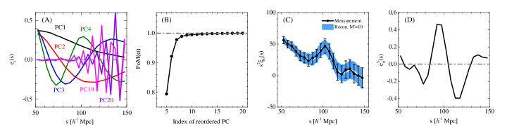
Figure 1: Panel (A): The first four (with largest variances) and the last two (with least variances) eigenvectors of the data covariance matrix for the monopole of the galaxy correlation function; (B): The forecasted FoM of the isotropic BAO parameter $\alpha$, as a function of the number of total reordered PC modes used. The FoM is normalized so that it is exactly $1$ if all the PC modes are used; (C): A comparison between the measured $\xi_{0}$ (black curves with the 68% CL error bars) and the reconstructed $\xi_{0}$ from the first ten PC modes (white curve with a blue band showing the 68% CL uncertainty); (D): The projection vector for the $\alpha$ parameter ${\bf e}_{\alpha}^{V}$, as defined in Eq (10).

As we shall demonstrate later, using a small fraction of the PC modes is sufficient to extract almost all the information we seek for a cosmological analysis. Moreover, the selected PC modes can further be compressed using the MOPED scheme, with almost no loss of information for the parameters we are interested in, and it can also highlight the key informative modes for the specific parameters we aim to constrain.

We seek a transformation matrix ${\bf V}$ that compresses the $\gamma$’s without loss of information, which means that the compressed data vector $\bf\Gamma^{V}$ contains the same information as $\bf\Gamma$; i.e.,

$${\bf\Gamma^{V}}\equiv{\bf V}^{T}{\bf\Gamma},\ {\bf\Gamma}\equiv\left[\gamma_{1},\gamma_{2},...,\gamma_{M^{\prime}}\right]^{T}\,.$$ (7)

Mathematically, this compression is lossless if the weighting vectors for multiple parameters $\{\theta_{1},\theta_{p>1}\}$ satisfy MOPED ,

$${\bf V}_{1} = \frac{\mathbf{\Lambda}^{-1}{\bf D}_{,1}}{\sqrt{{\bf D}_{,1}^{t}\mathbf{\Lambda}^{-1}{\bf D}_{,1}}}\,,~{}~{}{\bf D}_{,1}\equiv\frac{\partial\bf\Gamma}{\partial\theta_{1}}\,,$$ (8)

$${\bf V}_{p>1} = \frac{\mathbf{\Lambda}^{-1}{\bf D}_{,p}-\sum_{q=1}^{p-1}\left({\bf D}_{,p}^{t}\mathbf{V}_{q}\right)\mathbf{V}_{q}}{\sqrt{{\bf D}_{,p}\mathbf{\Lambda}^{-1}{\bf D}_{,p}-\sum_{q=1}^{m-1}\left({\bf D}_{,p}^{t}\mathbf{V}_{q}\right)^{2}}}\,,~{}~{}{\bf D}_{,p}\equiv\frac{\partial\bf\Gamma}{\partial\theta_{p}}\,,$$

Note that the weighting vectors are orthonormalized MOPED such that the compressed $\gamma$’s are uncorrelated and have unit variances Note that the compressed $\gamma$’s can also be obtained by a direct projection of the measured anisotropic correlation function $\xi({\bf s})$, e.g. , for a given parameter $p$,

$$\gamma_{p}^{V}={\bf e}_{p}^{V}\cdot\xi({\bf s}),\ \ {\bf e}_{p}^{V}\equiv\mathbf{V}_{p}{\bf e}.$$ (10)

The role of the vector ${\bf e}_{p}^{V}$ is to extract all the relevant information content for parameter $p$ from $\xi({\bf s})$ into one single number, thus the shape of $\gamma_{p}^{V}$ can be used for the optimization of galaxy surveys for the interesting parameters. It is straightforward to generalize to cases with multiple parameters, in which ${\bf e}^{V}$ has multiple columns (one for each parameter).

III Demonstration

Here we present a demonstration of the method we developed, using the mock and actual galaxy catalogs in the BOSS DR12 DR12 ; patchy . We start from a measurement of the isotropic BAO distance scale in a redshift range of $z\in[0.40,0.55]$, using $\xi_{0}$, the monopole of the CF. A BAO analysis in this redshift slice has been performed using the same galaxy sample Wang:2016wjr , which can be used for direct comparison.

We measure $\xi_{0}$ from $2048$ realizations of the MutliDark-Patchy mock catalogs patchy , from which we evaluate the data covariance matrix ${\bf C}$. We then perform a PCA of ${\bf C}$ using Eq. (1), and show the first four and the last two eigenvectors (ordered by the variances) in panel (A) of Fig. 1. As shown, the first few modes with the largest variances, which are expected to carry most of the signal in data, are rather smooth, while the last few noisy modes have the least variances.

We use the same template as in the DR12 analysis, i.e., $\smash{\xi_{0}^{\rm th}(s)=B^{2}\xi_{0}(\alpha s)+{a_{1}}/{s^{2}}+{a_{2}}/{s}+a_{3}}$, where $\smash{\alpha=\left[D_{V}(z)r_{d}^{\rm fid}\right]/\left[D^{\rm fid}_{V}(z)r_{d}\right]}$ is a dilation factor, describing a shift in the isotropic volume distance, $D_{V}(z)$. $B$ denotes the bias factor, and $a_{1},...,a_{3}$ are co-varied to marginalize over the broad-band shape. Instead of using $\xi_{0}$ as observables as in Wang:2016wjr , we use the $\gamma$’s, the coefficients of the PC modes. To determine how many PC modes are sufficient to extract most of the information for $\alpha$, we first perform a forecast using the Fisher matrix, with free parameters including $\smash{\mathbf{\Theta}\equiv\{\alpha,B^{2},a_{1-3}\}}$.

Observable	$N_{\rm data}$	Mocks	DR12 Galaxies
$\xi_{0}(s)$	$20$	$1.0033\pm 0.0229$	$1.0234\pm 0.0198$ Wang:2016wjr
$\gamma$’s	$10$	$1.0034\pm 0.0226$	$1.0224\pm 0.0201~{}~{}~{}~{}~{}\,$

Table 1: The constraints on $\alpha$ using $\xi_{0}$ and the PC modes as observables, respectively.

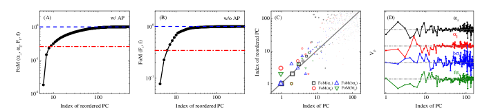
Figure 2: Panel (A): The FoM of $\{\alpha_{\bot},\alpha_{||},F_{1},f\}$ derived from various numbers of the total PC modes. The PC modes are re-ordered by the contribution of each mode to the FoM, and the FoM has been normalized so that it is unity using all the modes. The upper horizontal line shows the FoM using all the PC modes, and the lower line shows the FoM using the monopole and quadrupole only; (B): same as (A) but with $\alpha_{\bot}=\alpha_{||}=1$; (C): A scatter plot showing the correspondence between the re-ordered PC modes and the original PC modes. Different shapes represent the FoM for each parameter. For each parameter, the size of the symbols is proportional to the values of the FoM. The diagonal line shows the situation in which the modes ordered by the variance contribute to the FoM in the same order; (D): The optimal weights for various parameters, as shown in Eq. (8). The weights are arbitrarily offset for illustration, and the horizontal lines show ${\bf V}_{p}=0$.

We find that the original PC modes ordered by the variance of each mode, contribute to the Figure of Merit (FoM) defined as $1/\sqrt{\rm det\,Cov(\theta_{1},\theta_{2},...)}$ Albrecht:2009ct , following almost the same order. In Panel (B) of Fig. 1, we show the forecasted FoM of $\alpha$, which is simply $1/\sigma(\alpha)$, with other parameters marginalized over, as a function of the re-ordered PC modes. It is evident that the FoM starts to saturate with $\smash{M^{\prime}=10}$ modes, which is half of the total number of data points in the traditional analysis . A direct comparison of the constraint on $\alpha$ using these two approaches is presented in Table 1. As shown, the PCA approach returns almost an identical result to the traditional method, with the number of data points halved. This means that the last ten PC modes carry almost no information on $\alpha$, and they are also likely to be subject to observational systematics. A reconstruction of $\xi_{0}(s)$ using the first ten informative modes is shown in panel (C) of Fig. 1, which is a slightly smoothed version of the original measurement, with all the key features retained and uncertainty almost unchanged.

To illustrate where the key information for $\alpha$ stems from, we plot the projection vector ${\bf e}_{\alpha}^{V}$, which is introduced in Eq. (10), in panel (D) of Fig. 1. This vector effectively picks up information in $\xi_{0}$ in the range of $[80,130]\ h^{-1}\rm Mpc$ in a specific way, i.e., by contrasting $\xi_{0}$ around $105\ h^{-1}\rm Mpc$, where the BAO peaks.

In what follows, we consider the most general case, in which the anisotropic CF $\xi(s,\mu)$ is used as the raw observable, measured on a $\smash{N_{s}\times N_{\mu}}$ grid from the same BOSS DR12 catalogues, but in a wider redshift range ($\smash{0.5<z<0.75}$) to enhance the signal. Given the number of data points and mocks available, we chose to use a semi-analytic approach to estimate the data covariance matrix in the presence of a non-uniform survey window function, with the tool of RascalC Philcox et al.(2019) ; Philcox:2019ued . In this approach, the covariance matrix $\smash{C_{ij,k\ell}\equiv\langle\xi(s_{i},\mu_{j})\xi(s_{k},\mu_{\ell})\rangle-\langle\xi(s_{i},\mu_{j})\rangle\langle\xi(s_{k},\mu_{\ell})\rangle}$ is calculated using the galaxy and random catalogues as an input, with the non-Gaussian contribution approximated via a jackknife-rescaled inflation of shot-noise, which is shown to work well on cosmological analyses including the determination of the BAO scale. OConnell:2015src ; OConnell:2018oqr ; Philcox:2019ued .

As we did for $\xi_{0}$, we perform a PCA on $C_{ij,k\ell}$ using Eq. (1), and use the coefficients of the PC modes as observables to constrain BAO and RSD parameters in the set $\smash{\mathbf{\Theta}\equiv\{\alpha_{\perp},\alpha_{||},F_{1},f,F_{2},\sigma_{\rm FoG}\}}$, where the scaling parameters $\smash{\alpha_{\perp}\equiv\left(D_{A}r_{d}^{\rm fid}\right)/\left(D^{\rm fid}_{A}r_{d}\right)}$ and $\smash{\alpha_{||}\equiv\left(H^{\rm fid}r_{d}^{\rm fid}\right)/\left(Hr_{d}\right)}$ are introduced to account for the Alcock-Paczynski (AP) effect APtest , $D^{\rm fid}_{A}$ and $H^{\rm fid}$ are the angular diameter distance and Hubble expansion rate in the fiducial cosmology, respectively, and $r_{d}$ is the sound horizon scale at the drag epoch. The quantities $F_{1}$ and $F_{2}$ are the local Lagrangian bias parameters (the Eulerian linear bias $b$ is related by $\smash{b=1+F_{1}}$), $f$ is the linear growth rate, and $\sigma_{\rm FoG}$ is used to marginalize over the Fingers-of-God (FoG) effect on nonlinear scales. The Gaussian Streaming model is used to link theory to observables Reid:2011ar ; Reid et al.(2012) ,

$$1+\xi^{\rm th}(s_{\perp},s_{\parallel}) = \int\frac{{\rm d}y}{\sqrt{2\pi\left[\sigma^{2}_{12}(r,\mu)+\sigma^{2}_{\rm FoG}\right]}}\left[1+\xi(r)\right]$$ (11)

$$\times \exp\left\{-\frac{\left[s_{\parallel}-y-\mu v_{12}(r)\right]^{2}}{2\left[\sigma^{2}_{12}(r,\mu)+\sigma^{2}_{\rm FoG}\right]}\right\}\,,$$

where $\smash{s_{||}\equiv s\mu}$ and $\smash{s_{\perp}\equiv\sqrt{s(1-\mu^{2})}}$ denotes the separation of pairs along and across the LOS, respectively, $\xi(r)$ is the real-space CF as a function of the real-space separation $r$, $v_{12}(r)$ is the mean infall velocity of galaxies separated by $r$, and $\sigma_{12}(r,\mu)$ is the pairwise velocity dispersion of galaxies. The quantities $\xi(r)$, $v_{12}(r)$ and $\sigma_{12}(r,\mu)$ are computed using the Convolution Lagrangian Perturbation Theory (CLPT) Carlson:2012bu ; Wang:2013hwa .

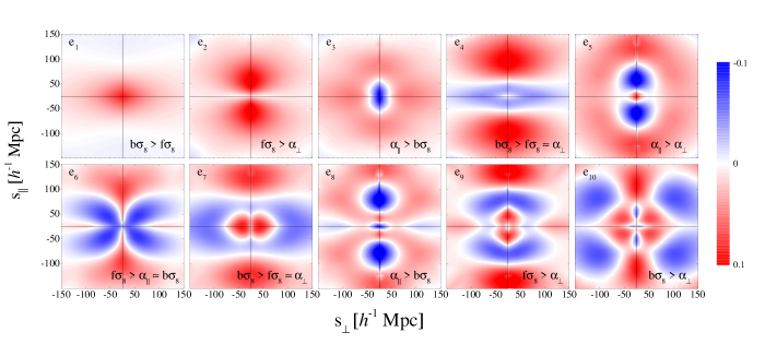
Figure 3: The first ten eigenvectors of the data covariance matrix for the anisotropic CF $\xi(s,\mu)$. To quantify the information content in each mode for the cosmological parameters, we use each PC mode to constrain the four parameters (one at a time), and compute the efficiency of each mode to constrain each of the parameters. For each mode, we show the most relevant parameter, followed by the one(s) that are less relevant. See text for more details.

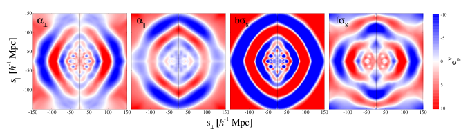
Figure 4: The optimal combinations of the PC modes, ${\bf e}_{p}^{V}$ defined in Eq. (10), that carry all the information for the BAO and RSD parameters, as illustrated in the legend.

	$\xi_{\rm MQH}$	$\xi(s,\mu)$
		PCA	PCA+MOPED
Mocks
$\Delta(\alpha_{\perp})$	$-0.008\pm 0.021$	$-0.002\pm 0.020$	$-0.004\pm 0.021$
$\Delta(\alpha_{\parallel})$	$\,\,\,\,0.014\pm 0.033$	$\,\,\,\,0.002\pm 0.031$	$\,\,\,\,0.005\pm 0.033$
$\Delta(f\sigma_{8})$	$-0.025\pm 0.041$	$-0.006\pm 0.042$	$-0.025\pm 0.042$
$\rm FoM$	$\,\,\,\,1.0$	$\,\,\,\,1.0$	$\,\,\,\,0.9$
$\rm Bias$	$\,\,\,\,1.0$	$\,\,\,\,0.22$	$\,\,\,\,0.87$
Samples
$\alpha_{\perp}$	$\,\,\,\,0.961\pm 0.024$	$\,\,\,\,0.976\pm 0.023$	$\,\,\,\,0.971\pm 0.025$
$\alpha_{\parallel}$	$\,\,\,\,1.034\pm 0.033$	$\,\,\,\,1.015\pm 0.030$	$\,\,\,\,1.020\pm 0.033$
$f\sigma_{8}$	$\,\,\,\,0.393\pm 0.046$	$\,\,\,\,0.408\pm 0.045$	$\,\,\,\,0.389\pm 0.043$
$\rm FoM$	$\,\,\,\,1.0$	$\,\,\,\,1.2$	$\,\,\,\,1.0$

Table 2: Mean and 68% CL uncertainty of the BAO and RSD parameters derived from the averaged mocks (upper part) and from the BOSS DR12 galaxy sample (lower). For the mock test, we show the deviation from the expected values. For each sample, results are shown using three kinds of observables: the monopole, quadrupole and hexadecapole ($\xi_{\rm MQH}$), the original PC modes derived from $\xi(s,\mu)$ (PCA), and the optimally combined PC modes (PCA+MOPED). The FoM and Bias are normalized using those derived from $\xi_{\rm MQH}$ so that ${\rm FoM}\ (\xi_{\rm MQH})={\rm Bias}\ (\xi_{\rm MQH})=1$.

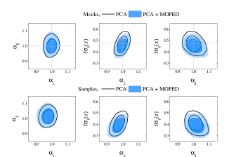
Figure 5: The 68 and 95% CL contours for the BAO and RSD parameters derived from the averaged mocks (upper panels) and from the BOSS DR12 galaxy sample (lower). Results using the original PC modes or the optimally combined modes as observables are shown with black unfilled contours and blue filled contours. Horizontal and vertical dashed lines in the upper panels illustrate the fiducial model of the mocks, which is expected to be consistent with the contours.

A Fisher forecast is performed to determine the number of modes required, before the actual data analysis. Panel (A) of Fig. 2 shows the FoM for parameters $\{\alpha_{\perp},\alpha_{||},F_{1},f\}$ as a function of numbers of the total PC modes used, and the modes are re-ordered by the contribution of each mode to the FoM. In panel (C) of Fig. 2, we plot the indices of the PC modes before and after the re-ordering, and find that the modes ordered by the variance, i.e., the original PC modes, contribute to the FoM following a similar order, which confirms that the noisy PC modes with the smallest eigen-values are least informative for a BAO and/or RSD analysis. As illustrated, the FoM grows quickly with the number of modes (e.g. , only $9$ modes are required to extract all the information in $\xi_{0}$ and $\xi_{2}$, which are measured in $50$ data points in the traditional method), and gets saturated with $\sim 150$ modes (only $\sim 25$ modes are needed if the AP effect is not considered, as shown in panel (B) of Fig. 2).

The first ten eigenvectors ($e_{1}$ to $e_{10}$) are shown in Fig. 3, and interesting patterns show up in these modes: (a) all the modes are anisotropic, reflecting the fact that they all contain information for the AP and RSD effect; (b) there is some level of isotropy on large scale ($s\gtrsim 100\ h^{-1}\ {\rm Mpc}$) in some modes, e.g. , $e_{3}$ and $e_{5}$, showing the impact of BAO; (c) the complexity of features increases with the index of modes, but a pattern exists, e.g. , $e_{1}$ has no node (it does not cross zero), $e_{2}$ has one node in the $s_{||}$ direction, $e_{3}$ has one node in both $s_{||}$ and $s_{\bot}$ directions, etc.

To associate these modes with the BAO/RSD parameters we are interested in, we compute the constraint of each mode on each individual parameters using the Fisher matrix technique, and identify the most relevant parameter(s) for each mode, i.e., the parameter(s) that are extracted with the highest efficiency from each PC mode. In practice, we first compute the FoM of each parameter using all the modes to define ${\rm FoM}_{\rm tot}$, the total information content for each parameter, then compute the efficacy of using the $i$th mode by evaluating ${\rm FoM}_{i}/{\rm FoM}_{\rm tot}$. In Fig. 3, the most relevant parameters are shown for each mode, e.g. , the apparently anisotropic modes $e_{1},e_{2},e_{4},e_{6},e_{7},e_{9}$ and $e_{10}$ are crucial to determine the RSD parameters $f\sigma_{8}$ and $b\sigma_{8}$, while the quasi-isotropic modes $e_{3},e_{5}$ and $e_{8}$ are more useful for $\alpha_{\bot}$ and $\alpha_{||}$.

As discussed previously, the PC modes can be optimally combined in a way such that all the information content for each parameter is stored in one single mode. We therefore compute the optimal weights using Eqs (8)-(10), and show the resultant modes for BAO and RSD parameters in Fig. 4, with coefficients for the PC modes, $V_{p}$, in panel (D) of Fig. 2. We can tell that for all the parameters, the first ten modes contribute the most to $|V_{p}|$, and $|V_{p}|$ quickly decays roughly after the $20$th mode. The parameter-specific modes in Fig. 4 are rather intuitive: the BAO/AP modes, denoted as $\alpha_{\bot}$ and $\alpha_{||}$, have clear ring-like structures, which are quasi-isotropic around the BAO scale, with an anisotropy therein to reflect the role of each parameter, i.e., the $\alpha_{\bot}$ and $\alpha_{||}$ mode shows a pattern of upweights across and along the LOS, respectively, which is as expected. The modes for $f\sigma_{8}$ and $b\sigma_{8}$, however, carry a high level of anisotropy, i.e., an obvious squashing pattern along the LOS, highlighting the RSD effect. These modes, upon which the observed $\xi(s,\mu)$ is projected for our analysis, along with the associated covariance matrix ${\bf C_{V}}$ defined in Eq. (7), contain all the information for the parameters of interest. We also present the weighted eigenvectors with respect to another parametrization for BAO, i.e.  the isotropic shift $\alpha$ and the anisotropic warping factor $\epsilon$ in Fig. 6 of the Appendix.

To demonstrate our method, we apply our pipeline on the BOSS DR12 mock and galaxy samples described earlier, and present the main results in Table 2 and Fig. 5. We constrain the BAO and RSD parameters using the original PC modes (up to $150$ PC modes, denoted as ‘PCA’), the optimally combined PC modes (denoted as ‘PCA+MOPED’), and the multipoles up to the hexadecapole (denoted as ‘$\xi_{\rm MQH}$’) for a comparison, respectively, and find that the results are largely consistent with each other. As demonstrated by the averaged mocks, with the PCA approach, we are able to extract all the information in $\xi_{0},\xi_{2}$ and $\xi_{4}$ quantified by the FoM using $150/500=30\%$ modes. Moreover, the Bias, which is the square root of the bias of all the parameters added in quadrature, can be significantly reduced by a factor 4.5 by the PCA method, largely due to the fact that the noisy modes are removed without loss of cosmological information. The PCA+MOPED approach, on the other hand, retains 90% the FoM, probably due to the fact that the probability distribution of some parameters such as $\sigma_{\rm FoG}$ are non-Gaussian, making the compression defined in Eq. (7) sub-optimal and thus subject to information loss to some extent. But even in this situation, the Bias is reduced by 17%. When applied to the BOSS DR12 sample, we find that the FoM extracted by the PC modes is 20% larger than that by the multipoles, and the PCA+MOPED approach is also subject to information loss compared to the PCA method, but it extracts all the information in the multipoles.

IV Conclusion and Discussions

In this era of precision cosmology, it is challenging to perform data analysis and cosmological implications for massive spectroscopic surveys, not only due to the large amount of observational data we are collecting, but also to the precision of measuring the cosmological parameters we require. This means that we need efficient and robust methods to extract cosmological information from galaxy surveys.

In this work, we develop a new method based on a principal component analysis for analyzing the anisotropic galaxy correlation functions $\xi(s,\mu)$. As we demonstrate using galaxy samples from BOSS DR12, our method is an ideal tool to meet our needs. A PCA of $\xi(s,\mu)$ can efficiently separate the cosmological signal we seek from the noise, which is non-informative. We confirm that most of the information for the BAO and RSD parameters, which are key for cosmological studies, is contained in the first few PC modes (the modes with the largest variances), making it natural to remove the PC modes with relatively small variances. Quantitatively, we find that using $150$ out of $500$ PC modes, one is able to recover all the information for a joint BAO and RSD study, and only $25$ out of $500$ modes are required for a RSD-only analysis. Being orthogonal to each other, the PC modes kept form a natural reservoir to store key information for general cosmological analysis, without redundancy.

To associate the PC modes with the parameters of interest, we optimally combine the PC modes using the MOPED compression scheme, so that all the information for each individual parameter is contained in one single mode. Thus the number of PC modes retained (i.e. 150 modes) can be reduced so that it is equal to the number of parameters of interest, i.e.  six parameters, with almost no loss of information. Our method and pipeline have been well validated using mock catalogs, and an application on the BOSS DR12 catalog shows that the FoM of BAO and RSD parameters is improved by $20\%$ compared to that using the traditional method.

Our method uses a mixture of simulations (for covariance matrix estimation) and analytic theory for the parameter dependence of the BAO and RSD effects. It therefore still depends to some extent on having a correct modeling for nonlinear effects. But the virtue of this framework is that it can be readily updated to incorporate revisions to theory. Our method provides an efficient way to extract the informative modes in the 2D correlation function and allows for a rapid estimation of BAO and RSD parameters from ongoing and forthcoming galaxy surveys including Dark Energy Spectroscopic Instrument (DESI) Aghamousa:2016zmz , the Euclid mission Laureijs:2011gra and the Subaru Prime Focus Spectrograph (PFS) Ellis:2012rn .

Appendix

Another parametrization for BAO is the isotropic shift $\alpha$ and the anisotropic warping factor $\epsilon$, which are defined in terms of $\alpha_{\perp}$ and $\alpha_{||}$, i.e.  $\alpha=\alpha_{\perp}^{2/3}\alpha_{||}^{1/3}$ and $\epsilon=(\alpha_{||}/\alpha_{\perp})^{1/3}-1$. The optimal combinations of PC modes for $\{\alpha,\epsilon,b\sigma_{8},f\sigma_{8}\}$ are shown in Fig. 6. It is seen that the $\alpha$ mode manifests a clear isotropic pattern. In contrast, the $\epsilon$ mode has an obvious anisotropy.

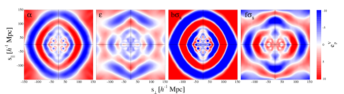
Figure 6: Same as Fig. 4, but for another BAO parametrization $\{\alpha,\epsilon$}.

References

- (1) S. Cole et al. [2dFGRS Collaboration], Mon. Not. Roy. Astron. Soc. 362 (2005) 505.
- (2) D. J. Eisenstein et al. [SDSS Collaboration], Astrophys. J. 633 (2005) 560.
- (3) Kaiser, N. 1987, Mon. Not. Roy. Astron. Soc. 227, 1
- (4) J. A. Peacock et al., Nature 410 (2001) 169.
- (5) Weinberg, D. H., Mortonson, M. J., Eisenstein, D. J., et al. 2013, Physics Reports, 530, 87.
- (6) K. Koyama, Rept. Prog. Phys. 79 (2016) no.4, 046902.
- (7) Blake, C., Glazebrook, K., Davis, T. M., et al. 2011, Mon. Not. Roy. Astron. Soc. , 418, 1725
- (8) S. Alam et al. [BOSS Collaboration], Mon. Not. Roy. Astron. Soc. 470 (2017) no.3, 2617.
- (9) M. Ata et al., Mon. Not. Roy. Astron. Soc. 473 (2018) no.4, 4773.
- (10) P. Zarrouk et al., Mon. Not. Roy. Astron. Soc. 477 (2018) no.2, 1639.
- (11) H. Gil-Marín et al., Mon. Not. Roy. Astron. Soc. 477 (2018) no.2, 1604.
- (12) G. B. Zhao et al., Mon. Not. Roy. Astron. Soc. 482 (2019) no.3, 3497.
- (13) A. Aghamousa et al. [DESI Collaboration], arXiv:1611.00036 [astro-ph.IM].
- (14) R. Laureijs et al. [EUCLID Collaboration], arXiv:1110.3193 [astro-ph.CO].
- (15) R. Ellis et al. [PFS Team], Publ. Astron. Soc. Jap. 66, no. 1, R1 (2014) doi:10.1093/pasj/pst019 [arXiv:1206.0737 [astro-ph.CO]].
- (16) W. J. Percival et al., arXiv:1903.03158 [astro-ph.CO].
- (17) A. J. Ross, W. J. Percival and M. Manera, Mon. Not. Roy. Astron. Soc. 451, no. 2, 1331 (2015).
- (18) D. Huterer and G. Starkman, Phys. Rev. Lett. 90, 031301 (2003).
- (19) R. G. Crittenden, L. Pogosian and G. B. Zhao, JCAP 0912, 025 (2009).
- (20) A. Heavens, R. Jimenez and O. Lahav, Mon. Not. Roy. Astron. Soc. 317 (2000), 965 doi:10.1046/j.1365-8711.2000.03692.x [arXiv:astro-ph/9911102 [astro-ph]].
- (21) S. Alam et al. [SDSS-III Collaboration], Astrophys. J. Suppl. 219, no. 1, 12 (2015).
- (22) F. S. Kitaura et al., Mon. Not. Roy. Astron. Soc. 456, no. 4, 4156 (2016).
- (23) M. Tegmark, A. Taylor and A. Heavens, Astrophys. J. 480, 22 (1997).
- (24) Y. Wang et al. [BOSS Collaboration], Mon. Not. Roy. Astron. Soc. 469 (2017) no.3, 3762.
- (25) A. Albrecht et al., arXiv:0901.0721 [astro-ph.IM].
- (26) Philcox, O. H. E., Eisenstein, D. J., O’Connell, R., et al. 2019, RascalC: Fast code for galaxy covariance matrix estimation, ascl:1909.008
- (27) O. H. E. Philcox, D. J. Eisenstein, R. O’Connell and A. Wiegand, arXiv:1904.11070 [astro-ph.CO].
- (28) R. O’Connell, D. Eisenstein, M. Vargas, S. Ho and N. Padmanabhan, Mon. Not. Roy. Astron. Soc. 462 (2016) no.3, 2681 doi:10.1093/mnras/stw1821 [arXiv:1510.01740 [astro-ph.CO]].
- (29) R. O’Connell and D. J. Eisenstein, Mon. Not. Roy. Astron. Soc. 487 (2019) no.2, 2701 doi:10.1093/mnras/stz1359 [arXiv:1808.05978 [astro-ph.CO]].
- (30) Alcock, C., & Paczynski, B. 1979, Nature, 281, 358
- (31) B. A. Reid and M. White, Mon. Not. Roy. Astron. Soc. 417 (2011) 1913.
- (32) Reid, B. A., Samushia, L., White, M., et al. 2012, Mon. Not. Roy. Astron. Soc. 426, 2719.
- (33) J. Carlson, B. Reid and M. White, Mon. Not. Roy. Astron. Soc. 429 (2013) 1674.
- (34) L. Wang, B. Reid and M. White, Mon. Not. Roy. Astron. Soc. 437 (2014) no.1, 588.