Adaptive Gradient Descent without Descent
 

Abstract

We present a strikingly simple proof that two rules are sufficient to automate gradient descent: 1) don’t increase the stepsize too fast and 2) don’t overstep the local curvature. No need for functional values, no line search, no information about the function except for the gradients. By following these rules, you get a method adaptive to the local geometry, with convergence guarantees depending only on the smoothness in a neighborhood of a solution. Given that the problem is convex, our method converges even if the global smoothness constant is infinity. As an illustration, it can minimize arbitrary continuously twice-differentiable convex function. We examine its performance on a range of convex and nonconvex problems, including logistic regression and matrix factorization.

1 Introduction

Since the early days of optimization it was evident that there is a need for algorithms that are as independent from the user as possible. First-order methods have proven to be versatile and efficient in a wide range of applications, but one drawback has been present all that time: the stepsize. Despite certain success stories, line search procedures and adaptive online methods have not removed the need to manually tune the optimization parameters. Even in smooth convex optimization, which is often believed to be much simpler than the nonconvex counterpart, robust rules for stepsize selection have been elusive. The purpose of this work is to remedy this deficiency.

The problem formulation that we consider is the basic unconstrained optimization problem

$$\min_{x\in\mathbb{R}^{d}}\ f(x),$$ (1)

where $f\colon\mathbb{R}^{d}\to\mathbb{R}$ is a differentiable function. Throughout the paper we assume that (1) has a solution and we denote its optimal value by $f_{*}$.

The simplest and most known approach to this problem is the gradient descent method (GD), whose origin can be traced back to Cauchy [9, 21]. Although it is probably the oldest optimization method, it continues to play a central role in modern algorithmic theory and applications. Its definition can be written in a mere one line,

$$x^{k+1}=x^{k}-\lambda\nabla f(x^{k}),\qquad k\geq 0,$$ (2)

where $x^{0}\in\mathbb{R}^{d}$ is arbitrary and $\lambda>0$. Under assumptions that $f$ is convex and $L$–smooth (equivalently, $\nabla f$ is $L$-Lipschitz) that is

$$\|\nabla f(x)-\nabla f(y)\|\leq L\|x-y\|,\quad\forall x,y,$$ (3)

one can show that GD with $\lambda\in(0,\frac{2}{L})$ converges to an optimal solution [31]. Moreover, with $\lambda=\frac{1}{L}$ the convergence rate [11] is

$$f(x^{k})-f_{*}\leq\frac{L\|x^{0}-x^{*}\|^{2}}{2(2k+1)},$$ (4)

where $x^{*}$ is any solution of (1). Note that this bound is not improvable [11].

We identify four important challenges that limit the applications of gradient descent even in the convex case:

1. GD is not general: many functions do not satisfy (3) globally.

2. GD is not a free lunch: one needs to guess $\lambda$, potentially trying many values before a success.

3. GD is not robust: failing to provide $\lambda<\frac{2}{L}$ may lead to divergence.

4. GD is slow: even if $L$ is finite, it might be arbitrarily larger than local smoothness.

1.1 Related work

Certain ways to address some of the issues above already exist in the literature. They include line search, adaptive Polyak’s stepsize, mirror descent, dual preconditioning, and stepsize estimation for subgradient methods. We discuss them one by one below, in a process reminiscent of cutting off Hydra’s limbs: if one issue is fixed, two others take its place.

The most practical and generic solution to the aforementioned issues is known as line search (or backtracking). This direction of research started from the seminal works [14] and [1] and continues to attract attention, see [5, 35] and references therein. In general, at each iteration the line search executes another subroutine with additional evaluations of $\nabla f$ and/or $f$ until some condition is met. Obviously, this makes each iteration more expensive.

At the same time, the famous Polyak’s stepsize [32] stands out as a very fast alternative to gradient descent. Furthermore, it does not depend on the global smoothness constant and uses the current gradient to estimate the geometry. The formula might look deceitfully simple, $\lambda_{k}=\frac{f(x^{k})-f_{*}}{\|\nabla f(x^{k})\|^{2}}$, but there is a catch: it is rarely possible to know $f_{*}$. This method, again, requires the user to guess $f_{*}$. What is more, with $\lambda$ it was fine to underestimate it by a factor of 10, but the guess for $f_{*}$ must be tight, otherwise it has to be reestimated later [16].

Seemingly no issue is present in the Barzilai-Borwein stepsize. Motivated by the quasi-Newton schemes, [3] suggested using steps

$$\lambda_{k}=\frac{\langle x^{k}-x^{k-1},\nabla f(x^{k})-\nabla f(x^{k-1})\rangle}{\|\nabla f(x^{k})-\nabla f(x^{k-1})\|^{2}}.$$

Alas, the convergence results regarding this choice of $\lambda_{k}$ are very limited and the only known case where it provably works is quadratic problems [33, 10]. In general it may not work even for smooth strongly convex functions, see the counterexample in [8].

Other more interesting ways to deal with non-Lipschitzness of $\nabla f$ use the problem structure. The first method, proposed in [7] and further developed in [4], shows that the mirror descent method [25], which is another extension of GD, can be used with a fixed stepsize, whenever $f$ satisfies a certain generalization of (3). In addition, [22] proposed the dual preconditioning method—another refined version of GD. Similarly to the former technique, it also goes beyond the standard smoothness assumption of $f$, but in a different way. Unfortunately, these two simple and elegant approaches cannot resolve all issues yet. First, not many functions fulfill respective generalized conditions. And secondly, both methods still get us back to the problem of not knowing the allowed range of stepsizes.

A whole branch of optimization considers adaptive extensions of GD that deal with functions whose (sub)gradients are bounded. Probably the earliest work in that direction was written by [36]. He showed that the method

$$x^{k+1}=x^{k}-\lambda_{k}\frac{g^{k}}{\|g^{k}\|},$$

where $g^{k}\in\partial f(x^{k})$ is a subgradient, converges for properly chosen sequences $(\lambda_{k})$, see, e.g., Section 3.2.3 in [28]. Moreover, $\lambda_{k}$ requires no knowledge about the function whatsoever.

Similar methods that work in online setting such as Adagrad [12, 24] received a lot of attention in recent years and remain an active topic of research [41]. Methods similar to Adagrad—Adam [19, 34], RMSprop [40] and Adadelta [42]—remain state-of-the-art for training neural networks. The corresponding objective is usually neither smooth nor convex, and the theory often assumes Lipschitzness of the function rather than of the gradients. Therefore, this direction of research is mostly orthogonal to ours, although we do compare with some of these methods in our neural networks experiment.

We also note that without momentum Adam and RMSprop reduce to signSGD [6], which is known to be non-convergent for arbitrary stepsizes on a simple quadratic problem [17].

In a close relation to ours is the recent work [23], where there was proposed an adaptive golden ratio algorithm for monotone variational inequalities. As it solves a more general problem, it does not exploit the structure of (1) and, as most variational inequality methods, has a more conservative update. Although the method estimates the smoothness, it still requires an upper bound on the stepsize as input.

Contribution.

We propose a new version of GD that at no cost resolves all aforementioned issues. The idea is simple, and it is surprising that it has not been yet discovered. In each iteration we choose $\lambda_{k}$ as a certain approximation of the inverse local Lipschitz constant. With such a choice, we prove that convexity and local smoothness of $f$ are sufficient for convergence of iterates with the complexity $\mathcal{O}(1/k)$ for $f(x^{k})-f_{*}$ in the worst case.

Discussion.

Let us now briefly discuss why we believe that proofs based on monotonicity and global smoothness lead to slower methods.

Gradient descent is by far not a recent method, so there have been obtained optimal rates of convergence. However, we argue that adaptive methods require rethinking optimality of the stepsizes. Take as an example a simple quadratic problem, $f(x,y)=\frac{1}{2}x^{2}+\frac{\delta}{2}y^{2}$, where $\delta\ll 1$. Clearly, the smoothness constant of this problem is equal to $L=1$ and the strong convexity one is $\mu=\delta$. If we run GD from an arbitrary point $(x^{0},y^{0})$ with the “optimal” stepsize $\lambda=\frac{1}{L}=1$, then one iteration of GD gives us $(x^{1},y^{1})=(0,(1-\delta)y^{0})$, and similarly $(x^{k},y^{k})=(0,(1-\delta)^{k}y^{0})$. Evidently for $\delta$ small enough it will take a long time to converge to the solution $(0,0)$. Instead GD would converge in two iterations if it adjusts its step after the first iteration to $\lambda=\frac{1}{\delta}$.

Nevertheless, all existing analyses of the gradient descent with $L$-smooth $f$ use stepsizes bounded by $2/L$. Besides, functional analysis gives

$$f(x^{k+1})\leq f(x^{k})-\lambda\Bigl{(}1-\frac{\lambda L}{2}\Bigr{)}\|\nabla f(x^{k})\|^{2},$$

from which $1/L$ can be seen as the “optimal” stepsize. Alternatively, we can assume that $f$ is $\mu$-strongly convex, and the analysis in norms gives

$$\|x^{k+1}-x^{*}\|^{2}\leq\Bigl{(}1-2\frac{\lambda L\mu}{L+\mu}\Bigr{)}\|x^{k}-x^{*}\|^{2}-\lambda\Bigl{(}\frac{2}{L+\mu}-\lambda\Bigr{)}\|\nabla f(x^{k})\|^{2},$$

whence the “optimal” step is $\frac{2}{L+\mu}$.

Finally, line search procedures use some certain type of monotonicity, for instance ensuring that $f(x^{k+1})\leq f(x^{k})-c\|\nabla f(x^{k})\|^{2}$ for some $c>0$. We break with this tradition and merely ask for convergence in the end.

2 Main part

2.1 Local smoothness of $f$

Recall that a mapping is locally Lipschitz if it is Lipschitz over any compact set of its domain. A function $f$ with (locally) Lipschitz gradient $\nabla f$ is called (locally) smooth. It is natural to ask whether some interesting functions are smooth locally, but not globally.

It turns out there is no shortage of examples, most prominently among highly nonlinear functions. In $\mathbb{R}$, they include $x\mapsto\exp(x)$, $\log(x)$, $\tan(x)$, $x^{p}$, for $p>2$, etc. More generally, they include any twice differentiable $f$, since $\nabla^{2}f(x)$, as a continuous mapping, is bounded over any bounded set $\mathcal{C}$. In this case, we have that $\nabla f$ is Lipschitz on $\mathcal{C}$, due to the mean value inequality

$$\|\nabla f(x)-\nabla f(y)\|\leq\max_{z\in\mathcal{C}}\|\nabla^{2}f(z)\|\|x-y\|,\quad\forall x,y\in\mathcal{C}.$$

Algorithm 1 that we propose is just a slight modification of GD. The quick explanation why local Lipschitzness of $\nabla f$ does not cause us any problems, unlike most other methods, lies in the way we prove its convergence. Whenever the stepsize $\lambda_{k}$ satisfies two inequalities

$$\begin{cases}\lambda_{k}^{2}&\leq(1+\theta_{k-1})\lambda_{k-1}^{2},\\ \lambda_{k}&\leq\frac{\|x^{k}-x^{k-1}\|}{2\|\nabla f(x^{k})-\nabla f(x^{k-1})\|},\end{cases}$$

independently of the properties of $f$ (apart from convexity), we can show that the iterates $(x^{k})$ remain bounded. Here and everywhere else we use the convention $1/0=+\infty$, so if $\nabla f(x^{k})-\nabla f(x^{k-1})=0$, the second inequality can be ignored. In the first iteration it might happen that $\lambda_{1}=\min\{+\infty\}$, in this case we suppose that any choice of $\lambda_{1}>0$ is possible.

Algorithm 1 Adaptive gradient descent

1:  Input: $x^{0}\in\mathbb{R}^{d}$, $\lambda_{0}>0$, $\theta_{0}=+\infty$

2:  $x^{1}=x^{0}-\lambda_{0}\nabla f(x^{0})$

3:  for $k=1,2,\dots$ do

4:     $\lambda_{k}=\min\Bigl{\{}\sqrt{1+\theta_{k-1}}\lambda_{k-1},\frac{\|x^{k}-x^{k-1}\|}{2\|\nabla f(x^{k})-\nabla f(x^{k-1})\|}\Bigr{\}}$

5:     $x^{k+1}=x^{k}-\lambda_{k}\nabla f(x^{k})$

6:     $\theta_{k}=\frac{\lambda_{k}}{\lambda_{k-1}}$

7:  end for

Although Algorithm 1 needs $x^{0}$ and $\lambda_{0}$ as input, this is not an issue as one can simply fix $x^{0}=0$ and $\lambda_{0}=10^{-10}$. Equipped with a tiny $\lambda_{0}$, we ensure that $x^{1}$ will be close enough to $x^{0}$ and likely will give a good estimate for $\lambda_{1}$. Otherwise, this has no influence on further steps.

2.2 Analysis without descent

It is now time to show our main contribution, the new analysis technique. The tools that we are going to use are the well-known Cauchy-Schwarz and convexity inequalities. In addition, our methods are related to potential functions [38], which is a powerful tool for producing tight bounds for GD.

Another divergence from the common practice is that our main lemma includes not only $x^{k+1}$ and $x^{k}$, but also $x^{k-1}$. This can be seen as a two-step analysis, while the majority of optimization methods have one-step bounds. However, as we want to adapt to the local geometry of our objective, it is rather natural to have two terms to capture the change in the gradients.

Now, it is time to derive a characteristic inequality for a specific Lyapunov energy.

Lemma 1.

Let $f\colon\mathbb{R}^{d}\to\mathbb{R}$ be convex and differential and let $x^{*}$ be any solution of (1). Then for $(x^{k})$ generated by Algorithm 1 it holds

$$\|x^{k+1}-x^{*}\|^{2}+\frac{1}{2}\|x^{k+1}-x^{k}\|^{2}+2\lambda_{k}(1+\theta_{k})(f(x^{k})-f_{*})\\ \leq\|x^{k}-x^{*}\|^{2}+\frac{1}{2}\|x^{k}-x^{k-1}\|^{2}+2\lambda_{k}\theta_{k}(f(x^{k-1})-f_{*}).$$ (5)

Proof.

Let $k\geq 1$. We start from the standard way of analyzing GD:

$$\|x^{k+1}-x^{*}\|^{2} =\|x^{k}-x^{*}\|^{2}+2\langle x^{k+1}-x^{k},x^{k}-x^{*}\rangle+\|x^{k+1}-x^{k}\|^{2}$$

$$=\|x^{k}-x^{*}\|^{2}+2\lambda_{k}\langle\nabla f(x^{k}),x^{*}-x^{k}\rangle+\|x^{k+1}-x^{k}\|^{2}.$$

As usually, we bound the scalar product by convexity of $f$:

$$2\lambda_{k}\langle\nabla f(x^{k}),x^{*}-x^{k}\rangle\leq 2\lambda_{k}(f_{*}-f(x^{k})),$$ (6)

which gives us

$$\|x^{k+1}-x^{*}\|^{2}\leq\|x^{k}-x^{*}\|^{2}-2\lambda_{k}(f(x^{k})-f_{*})+\|x^{k+1}-x^{k}\|^{2}.$$ (7)

These two steps have been repeated thousands of times, but now we continue in a completely different manner. We have precisely one “bad” term in (7), which is $\|x^{k+1}-x^{k}\|^{2}$. We will bound it using the difference of gradients:

$$\|x^{k+1}-x^{k}\|^{2} =2\|x^{k+1}-x^{k}\|^{2}-\|x^{k+1}-x^{k}\|^{2}=-2\lambda_{k}\langle\nabla f(x^{k}),x^{k+1}-x^{k}\rangle-\|x^{k+1}-x^{k}\|^{2}$$

$$=2\lambda_{k}\langle\nabla f(x^{k})-\nabla f(x^{k-1}),x^{k}-x^{k+1}\rangle$$

$$\qquad\qquad+2\lambda_{k}\langle\nabla f(x^{k-1}),x^{k}-x^{k+1}\rangle-\|x^{k+1}-x^{k}\|^{2}.$$ (8)

Let us estimate the first two terms in the right-hand side above. First, definition of $\lambda_{k}$, followed by Cauchy-Schwarz and Young’s inequalities, yields

$$2\lambda_{k}\langle\nabla f(x^{k})-\nabla f(x^{k-1}),x^{k}-x^{k+1}\rangle \leq 2\lambda_{k}\|\nabla f(x^{k})-\nabla f(x^{k-1})\|\|x^{k}-x^{k+1}\|$$

$$\leq\|x^{k}-x^{k-1}\|\|x^{k}-x^{k+1}\|$$

$$\leq\frac{1}{2}\|x^{k}-x^{k-1}\|^{2}+\frac{1}{2}\|x^{k+1}-x^{k}\|^{2}.$$ (9)

Secondly, by convexity of $f$,

$$2\lambda_{k}\langle\nabla f(x^{k-1}),x^{k}-x^{k+1}\rangle =\frac{2\lambda_{k}}{\lambda_{k-1}}\langle x^{k-1}-x^{k},x^{k}-x^{k+1}\rangle=2\lambda_{k}\theta_{k}\langle x^{k-1}-x^{k},\nabla f(x^{k})\rangle$$

$$\leq 2\lambda_{k}\theta_{k}(f(x^{k-1})-f(x^{k})).$$ (10)

Plugging (2.2) and (2.2) in (2.2), we obtain

$$\|x^{k+1}-x^{k}\|^{2}\leq\frac{1}{2}\|x^{k}-x^{k-1}\|^{2}-\frac{1}{2}\|x^{k+1}-x^{k}\|^{2}+2\lambda_{k}\theta_{k}(f(x^{k-1})-f(x^{k})).$$

Finally, using the produced estimate for $\|x^{k+1}-x^{k}\|^{2}$ in (7), we deduce the desired inequality (5). ∎

The above lemma already might give a good hint why our method works. From inequality (5) together with condition $\lambda_{k}^{2}\leq(1+\theta_{k-1})\lambda_{k-1}^{2}$, we obtain that the Lyapunov energy—the left-hand side of (5)—is decreasing. This gives us boundedness of $(x^{k})$, which is often the key ingredient for proving convergence. In the next theorem we formally state our result.

Theorem 1.

Suppose that $f\colon\mathbb{R}^{d}\to\mathbb{R}$ is convex with locally Lipschitz gradient $\nabla f$. Then $(x^{k})$ generated by Algorithm 1 converges to a solution of (1) and we have that

$$f(\hat{x}^{k})-f_{*}\leq\frac{D}{2S_{k}}=\mathcal{O}\Bigl{(}\frac{1}{k}\Bigr{)},$$

where

$$\hat{x}^{k} =\frac{\lambda_{k}(1+\theta_{k})x^{k}+\sum_{i=1}^{k-1}w_{i}x^{i}}{S_{k}},$$

$$w_{i} =\lambda_{i}(1+\theta_{i})-\lambda_{i+1}\theta_{i+1},$$

$$S_{k} =\lambda_{k}(1+\theta_{k})+\sum_{i=1}^{k-1}w_{i}=\sum_{i=1}^{k}\lambda_{i}+\lambda_{1}\theta_{1},$$

and $D$ is a constant that explicitly depends on the initial data and the solution set, see (11).

Our proof will consist of two parts. The first one is a straightforward application of Lemma 1, from which we derive boundedness of $(x^{k})$ and complexity result. Due to its conciseness, we provide it directly after this remark. In the second part, we prove that the whole sequence $(x^{k})$ converges to a solution. Surprisingly, this part is a bit more technical than expected, and thus we postpone it to the appendix.

Proof.

(Boundedness and complexity result.)

Fix any $x^{*}$ from the solution set of eq. 1. Telescoping inequality (5), we deduce

$$\|x^{k+1}-x^{*}\|^{2}+\frac{1}{2}\|x^{k+1}-x^{k}\|^{2}+2\lambda_{k}(1+\theta_{k})(f(x^{k})-f_{*})\\ +2\sum_{i=1}^{k-1}[\lambda_{i}(1+\theta_{i})-\lambda_{i+1}\theta_{i+1}](f(x^{i})-f_{*})\\ \leq\,\|x^{1}-x^{*}\|^{2}+\frac{1}{2}\|x^{1}-x^{0}\|^{2}+2\lambda_{1}\theta_{1}[f(x^{0})-f_{*}]\stackrel{{\scriptstyle\mathrm{def}}}{{=}}D.$$ (11)

Note that by definition of $\lambda_{k}$, the second line above is always nonnegative. Thus, the sequence $(x^{k})$ is bounded. Since $\nabla f$ is locally Lipschitz, it is Lipschitz continuous on bounded sets. It means that for the set $\mathcal{C}=\operatorname{\overline{conv}}\{x^{*},x^{0},x^{1},\dots\}$, which is bounded as the convex hull of bounded points, there exists $L>0$ such that

$$\|\nabla f(x)-\nabla f(y)\|\leq L\|x-y\|\quad\forall x,y\in\mathcal{C}.$$

Clearly, $\lambda_{1}=\frac{\|x^{1}-x^{0}\|}{2\|\nabla f(x^{1})-\nabla f(x^{0})\|}\geq\frac{1}{2L}$, thus, by induction one can prove that $\lambda_{k}\geq\frac{1}{2L}$, in other words, the sequence $(\lambda_{k})$ is separated from zero.

Now we want to apply the Jensen’s inequality for the sum of all terms $f(x^{i})-f_{*}$ in the left-hand side of (11). Notice, that the total sum of coefficients at these terms is

$$\lambda_{k}(1+\theta_{k})+\sum_{i=1}^{k-1}[\lambda_{i}(1+\theta_{i})-\lambda_{i+1}\theta_{i+1}]=\sum_{i=1}^{k}\lambda_{i}+\lambda_{1}\theta_{1}=S_{k}$$

Thus, by Jensen’s inequality,

$$\frac{D}{2}\geq\frac{\text{LHS of \eqref{eq:telescope}}}{2}\geq S_{k}(f(\hat{x}^{k})-f_{*}),$$

where $\hat{x}^{k}$ is given in the statement of the theorem. By this, the first part of the proof is complete. Convergence of $(x^{k})$ to a solution is provided in the appendix. ∎

As we have shown that $\lambda_{i}\geq\frac{1}{2L}$ for all $i$, we have a theoretical upper bound $f(\hat{x}^{k})-f_{*}\leq\frac{DL}{k}$. Note that in practice, however, $(\lambda_{k})$ might be much larger than the pessimistic lower bound $\frac{1}{2L}$, which we observe in our experiments together with a faster convergence.

2.3 $f$ is locally strongly convex

Since one of our goals is to make optimization easy to use, we believe that a good method should have state-of-the-art guarantees in various scenarios. For strongly convex functions, this means that we want to see linear convergence, which is not covered by normalized GD or online methods. In section 2.1 we have shown that Algorithm 1 matches the $\mathcal{O}(1/\varepsilon)$ complexity of GD on convex problems. Now we show that it also matches $\mathcal{O}(\frac{L}{\mu}\log\frac{1}{\varepsilon})$ complexity of GD when $f$ is locally strongly convex. Similarly to local smoothness, we call $f$ locally strongly convex if it is strongly convex over any compact set of its domain.

For proof simplicity, instead of using bound $\lambda_{k}\leq\sqrt{1+\theta_{k-1}}\lambda_{k-1}$ as in step 4 of Algorithm 1 we will use a more conservative bound $\lambda_{k}\leq\sqrt{1+\frac{\theta_{k-1}}{2}}\lambda_{k-1}$ (otherwise the derivation would be too technical). It is clear that with such a change Theorem 1 still holds true, so the sequence is bounded and we can rely on local smoothness and local strong convexity.

Theorem 2.

Suppose that $f\colon\mathbb{R}^{d}\to\mathbb{R}$ is locally strongly convex and $\nabla f$ is locally Lipschitz. Then $(x^{k})$ generated by Algorithm 1 (with the modification mentioned above) converges to the solution $x^{*}$ of (1). The complexity to get $\|x^{k}-x^{*}\|^{2}\leq\varepsilon$ is $\mathcal{O}(\kappa\log\frac{1}{\varepsilon})$, where $\kappa=\frac{L}{\mu}$ and $L,\mu$ are the smoothness and strong convexity constants of $f$ on the set $\mathcal{C}=\operatorname{\overline{conv}}\{x^{*},x^{0},x^{1},\dots\}$.

We want to highlight that in our rate $\kappa$ depends on the local Lipschitz and strong convexity constants $L$ and $\mu$, which is meaningful even when these properties are not satisfied globally. Similarly, if $f$ is globally smooth and strongly convex, our rate is still faster as it depends on the smaller local constants.

3 Heuristics

In this section, we describe several extensions of our method. We do not have a full theory for them, but believe that they are of interest in applications.

3.1 Acceleration

Algorithm 2 Adaptive accelerated gradient descent

1:  Input: $x^{0}\in\mathbb{R}^{d}$, $\lambda_{0}>0$, $\Lambda_{0}>0$, $\theta_{0}=\Theta_{0}=+\infty$

2:  $y^{1}=x^{1}=x^{0}-\lambda_{0}\nabla f(x^{0})$

3:  for $k=1,2,\dots$ do

4:     $\lambda_{k}=\min\Bigl{\{}\sqrt{1+\frac{\theta_{k-1}}{2}}\lambda_{k-1},\frac{\|x^{k}-x^{k-1}\|}{2\|\nabla f(x^{k})-\nabla f(x^{k-1})\|}\Bigr{\}}$

5:     $\Lambda_{k}=\min\Bigl{\{}\sqrt{1+\frac{\Theta_{k-1}}{2}}\Lambda_{k-1},\frac{\|\nabla f(x^{k})-\nabla f(x^{k-1})\|}{2\|x^{k}-x^{k-1}\|}\Bigr{\}}$

6:     $\beta_{k}=\frac{\sqrt{1/\lambda_{k}}-\sqrt{\Lambda_{k}}}{\sqrt{1/\lambda_{k}}+\sqrt{\Lambda_{k}}}$

7:     $y^{k+1}=x^{k}-\lambda_{k}\nabla f(x^{k})$

8:     $x^{k+1}=y^{k+1}+\beta_{k}(y^{k+1}-y^{k})$

9:     $\theta_{k}=\frac{\lambda_{k}}{\lambda_{k-1}}$, $\Theta_{k}=\frac{\Lambda_{k}}{\Lambda_{k-1}}$

10:  end for

Suppose that $f$ is $\mu$-strongly convex. One version of the accelerated gradient method proposed by Nesterov [28] is

$$y^{k+1} =x^{k}-\frac{1}{L}\nabla f(x^{k}),$$

$$x^{k+1} =y^{k+1}+\beta(y^{k+1}-y^{k}),$$

where $\beta=\frac{\sqrt{L}-\sqrt{\mu}}{\sqrt{L}+\sqrt{\mu}}$. Adaptive gradient descent for strongly convex $f$ efficiently estimated $\frac{1}{2L}$ by

$$\lambda_{k}=\min\biggl{\{}\sqrt{1+\frac{\theta_{k-1}}{2}}\lambda_{k-1},\frac{\|x^{k}-x^{k-1}\|}{2\|\nabla f(x^{k})-\nabla f(x^{k-1})\|}\biggr{\}}.$$

What about the strong convexity constant $\mu$? We know that it equals to the inverse smoothness constant of the conjugate $f^{*}(y)\stackrel{{\scriptstyle\mathrm{def}}}{{=}}\sup_{x}\{\langle x,y\rangle-f(x)\}$. Thus, it is tempting to estimate this inverse constant just as we estimated inverse smoothness of $f$, i.e., by formula

$$\Lambda_{k}=\min\biggl{\{}\sqrt{1+\frac{\Theta_{k-1}}{2}}\Lambda_{k-1},\frac{\|p^{k}-p^{k-1}\|}{2\|\nabla f^{*}(p^{k})-\nabla f^{*}(p^{k-1})\|}\biggr{\}}$$

where $p^{k}$ and $p^{k-1}$ are some elements of the dual space and $\Theta_{k}=\frac{\Lambda_{k}}{\Lambda_{k-1}}$. A natural choice then is $p^{k}=\nabla f(x^{k})$ since it is an element of the dual space that we use. What is its value? It is well known that $\nabla f^{*}(\nabla f(x))=x$, so we come up with the update rule

$$\Lambda_{k}=\min\biggl{\{}\sqrt{1+\frac{\Theta_{k-1}}{2}}\Lambda_{k-1},\frac{\|\nabla f(x^{k})-\nabla f(x^{k-1})\|}{2\|x^{k}-x^{k-1}\|}\biggr{\}},$$

and hence we can estimate $\beta$ by $\beta_{k}=\frac{\sqrt{1/\lambda_{k}}-\sqrt{\Lambda_{k}}}{\sqrt{1/\lambda_{k}}+\sqrt{\Lambda_{k}}}$.

We summarize our arguments in Algorithm 2. Unfortunately, we do not have any theoretical guarantees for it.

Estimating strong convexity parameter $\mu$ is important in practice. Most common approaches rely on restarting technique proposed by [26], see also [13] and references therein. Unlike Algorithm 2, these works have theoretical guarantees, however, the methods themselves are more complicated and still require tuning of other unknown parameters.

3.2 Uniting our steps with stochastic gradients

Here we would like to discuss applications of our method to the problem

$$\min_{x}\mathbb{E}\left[f_{\xi}(x)\right],$$

where $f_{\xi}$ is almost surely $L$-smooth and $\mu$-strongly convex. Assume that at each iteration we get sample $\xi^{k}$ to make a stochastic gradient step,

$$x^{k+1}=x^{k}-\lambda_{k}\nabla f_{\xi^{k}}(x^{k}).$$

Then, we have two ways of incorporating our stepsize into SGD. The first is to reuse $\nabla f_{\xi^{k}}(x^{k})$ to estimate $L_{k}=\frac{\|\nabla f_{\xi^{k}}(x^{k})-\nabla f_{\xi^{k}}(x^{k-1})\|}{\|x^{k}-x^{k-1}\|}$, but this would make $\lambda_{k}\nabla f_{\xi^{k}}(x^{k})$ biased. Alternatively, one can use an extra sample to estimate $L_{k}$, but this is less intuitive since our goal is to estimate the curvature of the function used in the update.

We give a full description in Algorithm 3. We remark that the option with a biased estimate performed much better in our experiments with neural networks. The theorem below provides convergence guarantees for both cases, but with different assumptions.

Algorithm 3 Adaptive SGD

1:  Input: $x^{0}\in\mathbb{R}^{d}$, $\lambda_{0}>0$, $\theta_{0}=+\infty$, $\xi^{0}$, $\alpha>0$

2:  $x^{1}=x^{0}-\lambda_{0}\nabla f_{\xi^{0}}(x^{0})$

3:  for $k=1,2,\dots$ do

4:     Sample $\xi^{k}$ and optionally $\zeta^{k}$

5:     Option I (biased): $L_{k}=\frac{\|\nabla f_{\xi^{k}}(x^{k})-\nabla f_{\xi^{k}}(x^{k-1})\|}{\|x^{k}-x^{k-1}\|}$

6:     Option II (unbiased): $L_{k}=\frac{\|\nabla f_{\zeta^{k}}(x^{k})-\nabla f_{\zeta^{k}}(x^{k-1})\|}{\|x^{k}-x^{k-1}\|}$

7:     $\lambda_{k}=\min\Bigl{\{}\sqrt{1+\theta_{k-1}}\lambda_{k-1},\frac{\alpha}{L_{k}}\Bigr{\}}$

8:     $x^{k+1}=x^{k}-\lambda_{k}\nabla f_{\xi^{k}}(x^{k})$

9:     $\theta_{k}=\frac{\lambda_{k}}{\lambda_{k-1}}$

10:  end for

Theorem 3.

Let $f_{\xi}$ be $L$-smooth and $\mu$-strongly convex almost surely. Assuming $\alpha\leq\frac{1}{2\kappa}$ and estimating $L_{k}$ with $\nabla f_{\zeta^{k}}$, the complexity to get $\mathbb{E}\left[\|x^{k}-x^{*}\|^{2}\right]\leq\varepsilon$ is not worse than $\mathcal{O}\left(\frac{\kappa^{2}}{\varepsilon}\log\frac{\kappa}{\varepsilon}\right)$. Furthermore, if the model is overparameterized, i.e., $\nabla f_{\xi}(x^{*})=0$ almost surely, then one can estimate $L_{k}$ with $\xi^{k}$ and the complexity is $\mathcal{O}\left(\kappa^{2}\log\frac{1}{\varepsilon}\right)$.

Note that in both cases we match the known dependency on $\varepsilon$ up to logarithmic terms, but we get an extra $\kappa$ as the price for adaptive estimation of the stepsize.

Another potential application of our techniques is estimation of decreasing stepsizes in SGD. The best known rates for SGD [37], are obtained using $\lambda_{k}$ that evolves as $\mathcal{O}\left(\frac{1}{L+\mu k}\right)$. This requires estimates of both smoothness and strong convexity, which can be borrowed from the previous discussion. We leave rigorous proof of such schemes for future work.

4 Experiments

In the experiments, we compare our approach with the two most related methods: GD and Nesterov’s accelerated method for convex functions [27]. Additionally, we consider line search, Polyak step, and Barzilai-Borwein method. For neural networks we also include a comparison with SGD, SGDm and Adam.

Logistic regression.

The logistic loss with $\ell_{2}$-regularization is given by $\frac{1}{n}\sum_{i=1}^{n}\log(1+\exp(-b_{i}a_{i}^{\top}x))+\frac{\gamma}{2}\|x\|^{2}$, where $n$ is the number of observations, $\gamma>0$ is a regularization parameter, and $(a_{i},b_{i})\in\mathbb{R}^{d}\times\mathbb{R}$, $i=1,\dots,n$, are the observations. We use ‘mushrooms’ and ‘covtype’ datasets to run the experiments. We choose $\gamma$ proportionally to $\frac{1}{n}$ as often done in practice. Since we have closed-form expressions to estimate $L=\frac{1}{4n}\|A\|^{2}+\gamma$, where $A=(a_{1}^{\top},\dotsc,a_{n}^{\top})^{\top}$, we used stepsize $\frac{1}{L}$ in GD and its acceleration. The results are provided in Figure 1.

Matrix factorization.

Given a matrix $A\in\mathbb{R}^{m\times n}$ and $r<\min\{m,n\}$, we want to solve $\min_{X=[U,V]}f(X)=f(U,V)=\frac{1}{2}\|UV^{\top}-A\|^{2}_{F}$ for $U\in\mathbb{R}^{m\times r}$ and $V\in\mathbb{R}^{n\times r}$. It is a nonconvex problem, and the gradient $\nabla f$ is not globally Lipschitz. With some tuning, one still can apply GD and Nesterov’s accelerated method, but—and we want to emphasize it—it was not a trivial thing to find the steps in practice. The steps we have chosen were almost optimal, namely, the methods did not converge if we doubled the steps. In contrast, our methods do not require any tuning, so even in this regard they are much more practical. For the experiments we used Movilens 100K dataset [15] with more than million entries and several values of $r=10,\ 20,\ 30$. All algorithms were initialized at the same point, chosen randomly. The results are presented in Figure 2.

Cubic regularization.

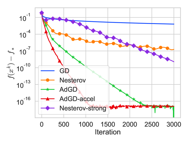
(a) Mushrooms dataset, objective

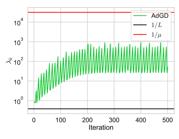
(b) Mushrooms dataset, stepsize

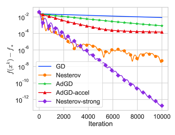
(c) Covtype dataset, objective

Figure 1: Results for the logistic regression problem.

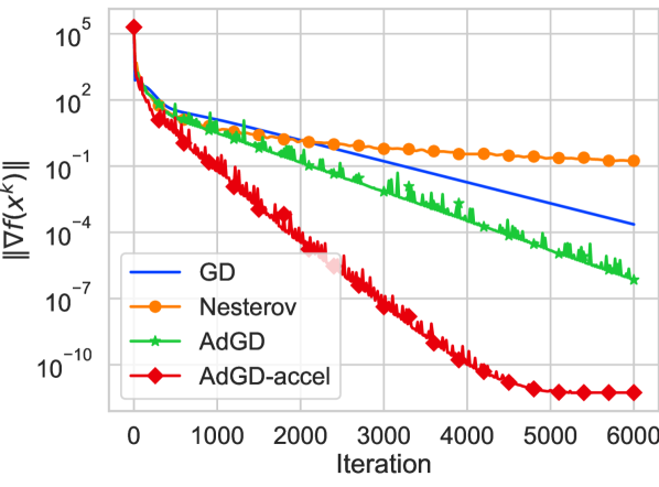
(a) $r=10$

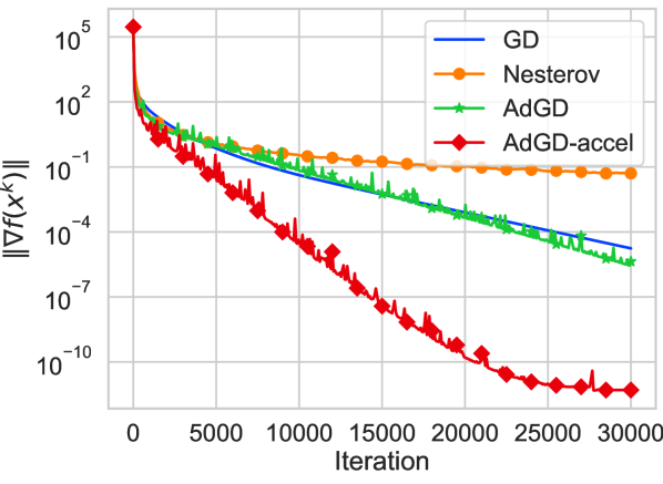
(b) $r=20$

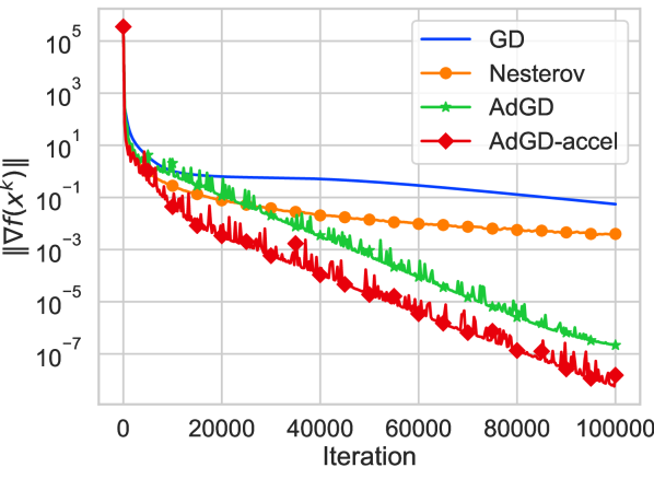
(c) $r=30$

Figure 2: Results for matrix factorization. The objective is neither convex nor smooth.

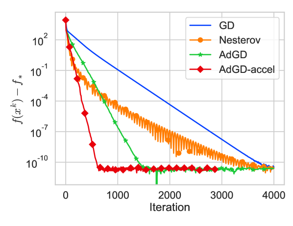
(a) $M=10$

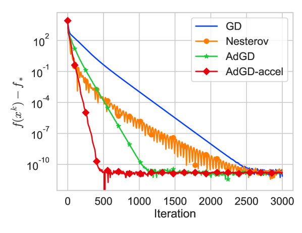
(b) $M=20$

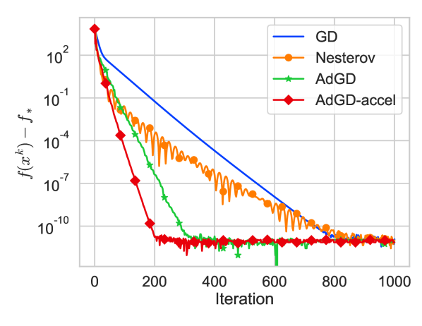
(c) $M=100$

Figure 3: Results for the non-smooth subproblem from cubic regularization.

In cubic regularization of Newton method [29], at each iteration we need to minimize $f(x)=g^{\top}x+\frac{1}{2}x^{\top}Hx+\frac{M}{6}\|x\|^{3}$, where $g\in\mathbb{R}^{d},H\in\mathbb{R}^{d\times d}$ and $M>0$ are given. This objective is smooth only locally due to the cubic term, which is our motivation to consider it. $g$ and $H$ were the gradient and the Hessian of the logistic loss with the ‘covtype’ dataset, evaluated at $x=0\in\mathbb{R}^{d}$. Although the values of $M=10$, $20$, $100$ led to similar results, they also required different numbers of iterations, so we present the corresponding results in Figure 3.

Barzilai-Borwein, Polyak and line searches.

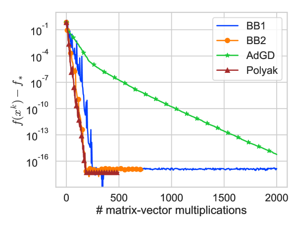
(a) Mushrooms dataset, objective

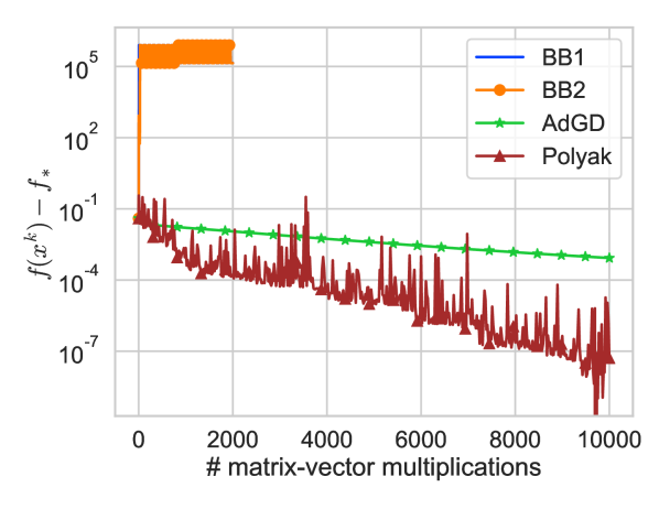
(b) Covtype dataset, objective

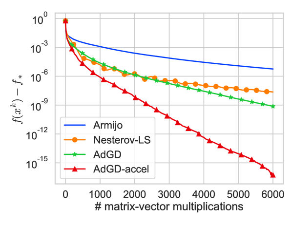
(c) W8a dataset, objective

Figure 4: Additional results for the logistic regression problem.

We have started this paper with an overview of different approaches to tackle the issue of a stepsize for GD. Now, we demonstrate some of those solutions. We again consider the $\ell_{2}$-regularized logistic regression (same setting as before) with ‘mushrooms’, ‘covtype’, and ‘w8a’ datasets.

In Figure 4 (left) we see that the Barzilai-Borwein method can indeed be very fast. However, as we said before, it lacks a theoretical basis and Figure 4 (middle) illustrates this quite well. Just changing one dataset to another makes both versions of this method to diverge on a strongly convex and smooth problem. Polyak’s method consistently performs well (see Figure 4 (left and middle)), however, only after it was fed with $f_{*}$ that we found by running another method. Unfortunately, for logistic regression there is no way to guess this value beforehand.

Finally, line search for GD (Armijo version) and Nesterov GD (implemented as in [26]) eliminates the need to know the stepsize, but this comes with a higher price per iteration as Figure 4 (right) shows. Actually in all our experiments for logistic regression with different datasets one iteration of Armijo line search was approximately 2 times more expensive than AdGD, while line search for Nesterov GD was 4 times more expensive. We note that these observations are consistent with the theoretical derivations in [26].

Neural networks.

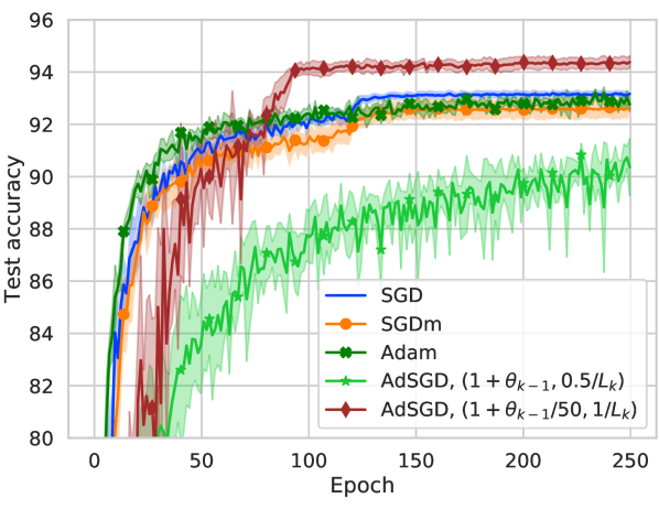
(a) Test accuracy

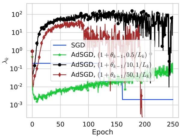
(b) Stepsize

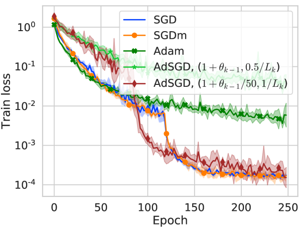
(c) Train loss

Figure 5: Results for training ResNet-18 on Cifar10. Labels for AdGD correspond to how $\lambda_{k}$ was estimated.

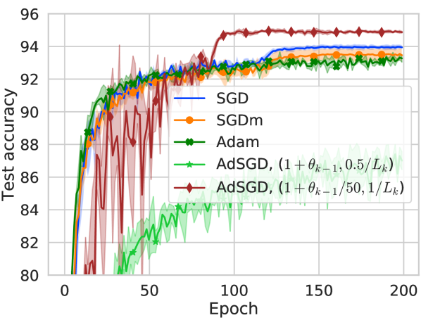
(a) Test accuracy

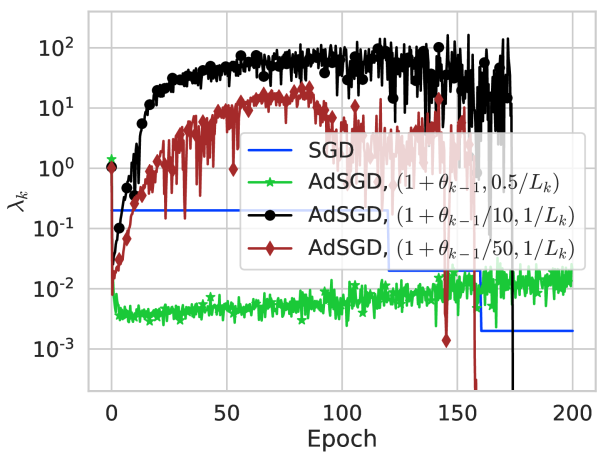
(b) Stepsize

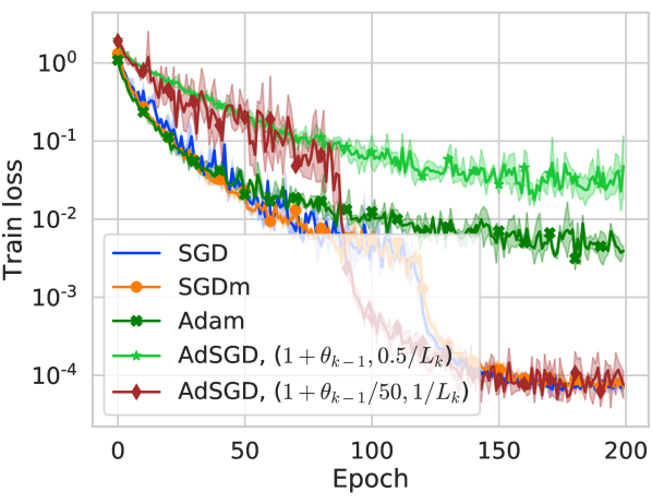
(c) Train loss

Figure 6: Results for training DenseNet-121 on Cifar10.

We use standard ResNet-18 and DenseNet-121 architectures implemented in PyTorch [30] and train them to classify images from the Cifar10 dataset [20] with cross-entropy loss.

We use batch size 128 for all methods. For our method, we observed that $\frac{1}{L_{k}}$ works better than $\frac{1}{2L_{k}}$. We ran it with $\sqrt{1+\gamma\theta_{k}}$ in the other factor with values of $\gamma$ from $\{1,0.1,0.05,0.02,\\ 0.01\}$ and $\gamma=0.02$ performed the best. For reference, we provide the result for the theoretical estimate as well and value $\gamma=0.1$ in the plot with estimated stepsizes. The results are depicted in Figures 5 and 6 and other details are provided in section 9.

We can see that, surprisingly, our method achieves better test accuracy than SGD despite having the same train loss. At the same time, our method is significantly slower at the early stage and the results are quite noisy for the first 75 epochs. Another observation is that the smoothness estimates are very non-uniform and $\lambda_{k}$ plummets once train loss becomes small.

5 Perspectives

We briefly provide a few directions which we personally consider to be important and challenging.

1. Nonconvex case. A great challenge for us is to obtain theoretical guarantees of the proposed method in the nonconvex settings. We are not aware of any generic first-order method for nonconvex optimization that does not rely on the descent lemma (or its generalization), see, e.g., [2].

2. Performance estimation. In our experiments we often observed much better performance of Algorithm 1, than GD or AGD. However, the theoretical rate we can show coincides with that of GD. The challenge here is to bridge this gap and we hope that the approach pioneered by [11] and further developed in [39, 18, 38] has a potential to do that.

3. Composite minimization. In classical first-order methods, the transition from smooth to composite minimization [26] is rather straightforward. Unfortunately, the proposed proof of Algorithm 1 does not seem to provide any route for generalization and we hope there is some way of resolving this issue.

4. Stochastic optimization. The derived bounds for the stochastic case are not satisfactory and have a suboptimal dependency on $\kappa$. However, it is not clear to us whether one can extend the techniques from the deterministic analysis to improve the rate.

5. Heuristics. Finally, we want to have some solid ground in understanding the performance of the proposed heuristics.

Acknowledgment.

Yura Malitsky wishes to thank Roman Cheplyaka for his interest in optimization that partly inspired the current work. Yura Malitsky was supported by the ONRG project N62909-17-1-2111 and HASLER project N16066.

Appendix:

6 Missing proofs

Recall that in the proof of Theorem 1 we only showed boundedness of the iterates and complexity for minimizing $f(x)$. It remains to show that sequence $(x^{k})$ converges to a solution. For this, we need some variation of the Opial lemma.

Lemma 2.

Let $(x^{k})$ and $(a_{k})$ be two sequences in $\mathbb{R}^{d}$ and $\mathbb{R}_{+}$ respectively. Suppose that $(x^{k})$ is bounded, its cluster points belong to $\mathcal{X}\subset\mathbb{R}^{d}$ and it also holds that

$$\|x^{k+1}-x\|^{2}+a_{k+1}\leq\|x^{k}-x\|^{2}+a_{k},\qquad\forall x\in\mathcal{X}.$$ (12)

Then $(x^{k})$ converges to some element in $\mathcal{X}$.

Proof.

Let $\bar{x}_{1}$, $\bar{x}_{2}$ be any cluster points of $(x^{k})$. Thus, there exist two subsequences $(x^{k_{i}})$ and $(x^{k_{j}})$ such that $x^{k_{i}}\to\bar{x}_{1}$ and $x^{k_{j}}\to\bar{x}_{2}$. Since $\|x^{k}-x\|^{2}+a_{k}$ is nonnegative and bounded, $\lim_{k\to\infty}(\|x^{k}-x\|^{2}+a_{k})$ exists for any $x\in\mathcal{X}$. Let $x=\bar{x}_{1}$. This yields

$$\lim_{k\to\infty}(\|x^{k}-\bar{x}_{1}\|^{2}+a_{k}) =\lim_{i\to\infty}(\|x^{k_{i}}-\bar{x}_{1}\|^{2}+a_{k_{i}})=\lim_{i\to\infty}a_{k_{i}}$$

$$=\lim_{j\to\infty}(\|x^{k_{j}}-\bar{x}_{1}\|^{2}+a_{k_{j}})=\|\bar{x}_{2}-\bar{x}_{1}\|^{2}+\lim_{j\to\infty}a_{k_{j}}.$$

Hence, $\lim_{i\to\infty}a_{k_{i}}=\lim_{j\to\infty}a_{k_{j}}+\|\bar{x}_{1}-\bar{x}_{2}\|^{2}$. Doing the same with $x=\bar{x}_{2}$ instead of $x=\bar{x}_{1}$, yields $\lim_{j\to\infty}a_{k_{j}}=\lim_{i\to\infty}a_{k_{i}}+\|\bar{x}_{1}-\bar{x}_{2}\|^{2}$. Thus, we obtain that $\bar{x}_{1}=\bar{x}_{2}$, which finishes the proof. ∎

Another statement that we need here is the following tightening of the convexity property.

Lemma 3 (Theorem 2.1.5, [28]).

Let $\mathcal{C}$ be a closed convex set in $\mathbb{R}^{d}$. If $f\colon\mathcal{C}\to\mathbb{R}$ is convex and $L$-smooth, then $\forall x,y\in\mathcal{C}$ it holds

$$f(x)-f(y)-\langle\nabla f(y),x-y\rangle\geq\frac{1}{2L}\|\nabla f(x)-\nabla f(y)\|^{2}.$$ (13)

Proof of Theorem 1.

(Convergence of $(x^{k})$)

Note that in the first part we have already proved that $(x^{k})$ is bounded and that $\nabla f$ is $L$-Lipschitz on $\mathcal{C}=\operatorname{\overline{conv}}\{x^{*},x^{0},x^{1},\dots\}$. Invoking Lemma 3, we deduce that

$$\lambda_{k}(f(x^{*})-f(x^{k}))\geq\lambda_{k}\langle\nabla f(x^{k}),x^{*}-x^{k}\rangle+\frac{\lambda_{k}}{2L}\|\nabla f(x^{k})\|^{2}.$$ (14)

This indicates that instead of using inequality (6) in the proof of Lemma 1, we could use a better estimate (14). However, we want to emphasize that we did not assume that $\nabla f$ is globally Lipschitz, but rather obtained Lipschitzness on $\mathcal{C}$ as an artifact of our analysis. Clearly, in the end this improvement gives us an additional term $\frac{\lambda_{k}}{L}\|\nabla f(x^{k})\|^{2}$ in the left-hand side of (5), that is

$$\|x^{k+1}-x^{*}\|^{2}+\frac{1}{2}\|x^{k+1}-x^{k}\|^{2}+2\lambda_{k}(1+\theta_{k})(f(x^{k})-f_{*})+\frac{\lambda_{k}}{L}\|\nabla f(x^{k})\|^{2}\\ \leq\|x^{k}-x^{*}\|^{2}+\frac{1}{2}\|x^{k}-x^{k-1}\|^{2}+2\lambda_{k}\theta_{k}(f(x^{k-1})-f_{*}).$$ (15)

Thus, telescoping (15), one obtains that $\sum_{i=1}^{k}\frac{\lambda_{k}}{L}\|\nabla f(x^{k})\|^{2}\leq D$. As $\lambda_{k}\geq\frac{1}{2L}$, one has that $\nabla f(x^{k})\to 0$. Now we might conclude that all cluster points of $(x^{k})$ are solutions of (1).

Let $\mathcal{X}$ be the solution set of (1) and $a_{k}=\frac{1}{2}\|x^{k}-x^{k-1}\|^{2}+2\lambda_{k}\theta_{k}(f(x^{k-1})-f_{*})$. We want to finish the proof applying Lemma 2. To this end, notice that inequality (5) yields (12), since $\lambda_{k+1}\theta_{k+1}\leq(1+\theta_{k})\lambda_{k}$. This completes the proof. ∎

Proof of Theorem 2.

First of all, we note that using the stricter inequality $\lambda_{k}\leq\sqrt{1+\frac{\theta_{k-1}}{2}}\lambda_{k-1}$ does not change the statement of Theorem 1. Hence, $x^{k}\to x^{*}$ and there exist $\mu,L>0$ such that $f$ is $\mu$-strongly convex and $\nabla f$ is $L$-Lipschitz on $\mathcal{C}=\operatorname{\overline{conv}}\{x^{*},x^{0},x^{1},\dots\}$. Secondly, due to local strong convexity, $\|\nabla f(x^{k})-\nabla f(x^{k-1})\|\geq\mu\|x^{k}-x^{k-1}\|$, and hence $\lambda_{k}\leq\frac{1}{2\mu}$ for $k\geq 1$.

Now we tighten some steps in the analysis to improve bound (6). By strong convexity,

$$\lambda_{k}\langle\nabla f(x^{k}),x^{*}-x^{k}\rangle \leq\lambda_{k}(f(x^{*})-f(x^{k}))-\lambda_{k}\frac{\mu}{2}\|x^{*}-x^{k}\|^{2}.$$

By $L$-smoothness and bound $\lambda_{k}\leq\frac{1}{2\mu}$,

$$\lambda_{k}\langle\nabla f(x^{k}),x^{*}-x^{k}\rangle \leq\lambda_{k}(f(x^{*})-f(x^{k}))-\lambda_{k}\frac{1}{2L}\|\nabla f(x^{k})\|^{2}$$

$$=\lambda_{k}(f_{*}-f(x^{k}))-\frac{1}{2L\lambda_{k}}\|x^{k+1}-x^{k}\|^{2}$$

$$\leq\lambda_{k}(f_{*}-f(x^{k}))-\frac{\mu}{L}\|x^{k+1}-x^{k}\|^{2}.$$

Together, these two bounds give us

$$\lambda_{k}\langle\nabla f(x^{k}),x^{*}-x^{k}\rangle \leq\lambda_{k}(f_{*}-f(x^{k}))-\lambda_{k}\frac{\mu}{4}\|x^{k}-x^{*}\|^{2}-\frac{\mu}{2L}\|x^{k+1}-x^{k}\|^{2}.$$

We keep inequality (2.2) and the rest of the proof as is. Then the strengthen analog of (5) will be

$$\|x^{k+1}-x^{*}\|^{2}+\frac{1}{2}\left(1+\frac{2\mu}{L}\right)\|x^{k+1}-x^{k}\|^{2}+2\lambda_{k}(1+\theta_{k})(f(x^{k})-f_{*})$$

$$\leq\, \left(1-\frac{\lambda_{k}\mu}{2}\right)\|x^{k}-x^{*}\|^{2}+\frac{1}{2}\|x^{k}-x^{k-1}\|^{2}+2\lambda_{k}\theta_{k}(f(x^{k-1})-f_{*})$$

$$\leq\, \left(1-\frac{\lambda_{k}\mu}{2}\right)\|x^{k}-x^{*}\|^{2}+\frac{1}{2}\|x^{k}-x^{k-1}\|^{2}+2\lambda_{k-1}\left(1+\frac{\theta_{k-1}}{2}\right)(f(x^{k-1})-f_{*}),$$ (16)

where in the last inequality we used our new condition on $\lambda_{k}$. Under the new update we have contraction in every term: $1-\frac{\lambda_{k}\mu}{2}$ in the first, $\frac{1}{1+2\mu/L}=1-\frac{2\mu}{L+2\mu}$ in the second and $\frac{1+\theta_{k-1}/2}{1+\theta_{k-1}}=1-\frac{\theta_{k-1}}{2(1+\theta_{k-1})}$ in the last one.

To further bound the last contraction, recall that $\lambda_{k}\in\left[\frac{1}{2L},\frac{1}{2\mu}\right]$ for $k\geq 1$. Therefore, $\theta_{k}=\frac{\lambda_{k}}{\lambda_{k-1}}\geq\frac{1}{\kappa}$ for any $k>1$, where $\kappa\stackrel{{\scriptstyle\mathrm{def}}}{{=}}\frac{L}{\mu}$. Since the function $\theta\mapsto\frac{\theta}{1+\theta}$ monotonically increases with $\theta>0$, this implies $\frac{\theta_{k-1}}{2(1+\theta_{k-1})}\geq\frac{1}{2(\kappa+1)}$ when $k>2$. Thus, for the full energy $\Psi^{k+1}$ (the left-hand side of (16)) we have

$$\Psi^{k+1} \leq\left(1-\min\left\{\frac{\lambda_{k}\mu}{2},\frac{1}{2(\kappa+1)},\frac{2\mu}{L+2\mu}\right\}\right)\Psi^{k}.$$

Using simple bounds $\frac{\lambda_{k}\mu}{2}\geq\frac{1}{4\kappa}$, $\frac{2\mu}{L+2\mu}=\frac{2}{\kappa+2}\geq\frac{1}{4\kappa}$, and $\frac{1}{2(\kappa+1)}\geq\frac{1}{4\kappa}$, we obtain $\Psi^{k+1}\leq(1-\frac{1}{4\kappa})\Psi^{k}$ for $k>2$. This gives $\mathcal{O}\left(\kappa\log\frac{1}{\varepsilon}\right)$ convergence rate. ∎

7 Extensions

7.1 More general update

One may wonder how flexible the update for $\lambda_{k}$ in Algorithm 1 is? For example, is it necessary to upper bound the stepsize with $\sqrt{1+\theta_{k}}\lambda_{k-1}$ and put $2$ in the denominator of $\frac{\|x^{k}-x^{k-1}\|}{2\|\nabla f(x^{k})-\nabla f(x^{k-1})\|}$? Algorithm 4 that we present here partially answers this question.

Algorithm 4 Adaptive gradient descent (general update)

1:  Input: $x^{0}\in\mathbb{R}^{d}$, $\lambda_{0}>0$, $\theta_{0}=+\infty$, $\alpha\in(0,1)$, $\beta=\frac{1}{2(1-\alpha)}$

2:  $x^{1}=x^{0}-\lambda_{0}\nabla f(x^{0})$

3:  for $k=1,2,\dots$ do

4:     $\lambda_{k}=\min\Bigl{\{}\sqrt{\frac{1}{\beta}+\theta_{k-1}}\lambda_{k-1},\frac{\alpha\|x^{k}-x^{k-1}\|}{\|\nabla f(x^{k})-\nabla f(x^{k-1})\|}\Bigr{\}}$

5:     $x^{k+1}=x^{k}-\lambda_{k}\nabla f(x^{k})$

6:     $\theta_{k}=\frac{\lambda_{k}}{\lambda_{k-1}}$

7:  end for

Obviously, Algorithm 1 is a particular case of Algorithm 4 with $\alpha=\frac{1}{2}$ and $\beta=1$.

Theorem 4.

Suppose that $f\colon\mathbb{R}^{d}\to\mathbb{R}$ is convex with locally Lipschitz gradient $\nabla f$. Then $(x^{k})$ generated by Algorithm 4 converges to a solution of (1) and we have that

$$f(\hat{x}^{k})-f_{*}\leq\frac{D}{2S_{k}}=\mathcal{O}\Bigl{(}\frac{1}{k}\Bigr{)},$$

where

$$\hat{x}^{k} =\frac{\lambda_{k}(1+\theta_{k}\beta)x^{k}+\sum_{i=1}^{k-1}w_{i}x^{i}}{S_{k}},$$

$$w_{i} =\lambda_{i}(1+\theta_{i}\beta)-\lambda_{i+1}\theta_{i+1}\beta,$$

$$S_{k} =\lambda_{k}(1+\theta_{k}\beta)+\sum_{i=1}^{k-1}w_{i}=\sum_{i=1}^{k}\lambda_{i}+\lambda_{1}\theta_{1}\beta,$$

and $D$ is a constant that explicitly depends on the initial data and the solution set.

Proof.

Let $x^{*}$ be arbitrary solution of (1). We note that equations (7) and (2.2) hold for any variant of GD, independently of $\lambda_{k}$, $\alpha$, $\beta$. With the new rule for $\lambda_{k}$, from (2.2) it follows

$$\|x^{k+1}-x^{k}\|^{2} \leq 2\lambda_{k}\theta_{k}(f(x^{k-1})-f(x^{k}))-\|x^{k+1}-x^{k}\|^{2}+2\lambda_{k}\|\nabla f(x^{k})-\nabla f(x^{k-1})\|\|x^{k}-x^{k+1}\|$$

$$\leq 2\lambda_{k}\theta_{k}(f(x^{k-1})-f(x^{k}))-(1-\alpha)\|x^{k+1}-x^{k}\|^{2}+\alpha\|x^{k}-x^{k-1}\|^{2},$$

which, after multiplication by $\beta$ and reshuffling the terms, becomes

$$\beta(2-\alpha)\|x^{k+1}-x^{k}\|^{2}+2\beta\lambda_{k}\theta_{k}(f(x^{k})-f_{*})\leq\alpha\beta\|x^{k}-x^{k-1}\|^{2}+2\beta\lambda_{k}\theta_{k}(f(x^{k-1})-f_{*}).$$

Adding (7) and the latter inequality gives us

$$\|x^{k+1}-x^{*}\|^{2}+2\lambda_{k}(1+\theta_{k}\beta)(f(x^{k})-f_{*})+(2\beta-\alpha\beta-1)\|x^{k+1}-x^{k}\|^{2}$$

$$\leq\|x^{k}-x^{*}\|^{2}+2\lambda_{k}\theta_{k}\beta(f(x^{k-1})-f_{*})+\alpha\beta\|x^{k+1}-x^{k}\|^{2}.$$

Notice that by $\beta=\frac{1}{2(1-\alpha)}$, we have $2\beta-\alpha\beta-1=\alpha\beta$ and hence,

$$\|x^{k+1}-x^{*}\|^{2}+2\lambda_{k}(1+\theta_{k}\beta)(f(x^{k})-f_{*})+\alpha\beta\|x^{k+1}-x^{k}\|^{2}$$

$$\leq\|x^{k}-x^{*}\|^{2}+2\lambda_{k}\theta_{k}\beta(f(x^{k-1})-f_{*})+\alpha\beta\|x^{k+1}-x^{k}\|^{2}.$$

As a sanity check, we can see that with $\alpha=\frac{1}{2}$ and $\beta=1$, the above inequality coincides with (5).

Telescoping this inequality, we deduce

$$\|x^{k+1}-x^{*}\|^{2} +\alpha\beta\|x^{k+1}-x^{k}\|^{2}+2\lambda_{k}(1+\theta_{k}\beta)(f(x^{k})-f_{*})$$

$$\qquad+2\sum_{i=1}^{k-1}[\lambda_{i}(1+\theta_{i}\beta)-\lambda_{i+1}\theta_{i+1}\beta](f(x^{i})-f_{*})$$

$$\leq\|x^{1}-x^{*}\|^{2}+\alpha\beta\|x^{1}-x^{0}\|^{2}+2\lambda_{1}\theta_{1}\beta[f(x^{0})-f_{*}]\stackrel{{\scriptstyle\mathrm{def}}}{{=}}D.$$ (17)

Note that because of the way we defined stepsize, $\lambda_{i}(1+\theta_{i}\beta)-\lambda_{i+1}\theta_{i+1}\beta\geq 0$. Thus, the sequence $(x^{k})$ is bounded. Since $\nabla f$ is locally Lipschitz, it is Lipschitz continuous on bounded sets. Let $L$ be a Lipschitz constant of $\nabla f$ on a bounded set $\mathcal{C}=\operatorname{\overline{conv}}\{x^{*},x^{1},x^{2},\dots\}$.

If $\alpha\leq\frac{1}{2}$, then $\frac{1}{\beta}>1$ and similarly to Theorem 1 we might conclude that $\lambda_{k}\geq\frac{\alpha}{L}$ for all $k$. However, for the case $\alpha>\frac{1}{2}$ we cannot do this. Instead, we prove that $\lambda_{k}\geq\frac{2\alpha(1-\alpha)}{L}$, which suffices for our purposes.

Let $m,n\in\mathbb{N}$ be the smallest numbers such that $\beta^{-\frac{1}{2^{m}}}\geq 1-\frac{1}{2\beta}$ and $(1+\frac{1}{\beta})^{\frac{n}{2}}\geq\beta$. We want to prove that for any $k$ it holds $\lambda_{k}\geq\frac{2\alpha(1-\alpha)}{L}$ and among every $m+n+1$ consecutive elements $\lambda_{k},\lambda_{k+1},\dots,\lambda_{k+m+n}$ at least one is no less than $\frac{\alpha}{L}$. We shall prove this by induction. First, note that the second bound always satisfies $\frac{\alpha\|x^{k}-x^{k-1}\|}{\|\nabla f(x^{k})-\nabla f(x^{k-1})\|}\geq\frac{\alpha}{L}$ for all $k$, which also implies that $\lambda_{1}\geq\frac{\alpha}{L}$. If for all $k$ we have $\lambda_{k}\geq\frac{\alpha}{L}$, then we are done. Now assume that $\lambda_{k-1}\geq\frac{\alpha}{L}$ and $\lambda_{k}<\frac{\alpha}{L}$ for some $k$. Choose the largest $j$ (possibly infinite) such that the second bound is not active for $\lambda_{k},\dotsc,\lambda_{k+j-1}$, i.e., $\lambda_{k+i}=\sqrt{\frac{1}{\beta}+\theta_{k+i-i}}\lambda_{k+i-1}$ for $i<j$.

Let us prove that $\lambda_{k},\dotsc,\lambda_{k+j-1}\geq\frac{2\alpha(1-\alpha)}{L}$. The definition of $j$ yields $\theta_{k+i}=\sqrt{\frac{1}{\beta}+\theta_{k+i-1}}$ for all $i=0,\dots,j-1$. Recall that $\beta>1$, and thus,

$$\theta_{k}\geq\beta^{-\frac{1}{2}},\quad\theta_{k+1}\geq\sqrt{\frac{1}{\beta}+\sqrt{\frac{1}{\beta}}}\geq\beta^{-\frac{1}{4}},\quad\dotsc,\quad\theta_{k+i}\geq\sqrt{\frac{1}{\beta}+\beta^{-\frac{1}{2^{i}}}}\geq\beta^{-\frac{1}{2^{i+1}}}$$

for all $i<j$. Now it remains to notice that for any $i<j$

$$\frac{\lambda_{k+i}}{\lambda_{k-1}}=\theta_{k}\theta_{k+1}\dots\theta_{k+i}\geq\beta^{-\frac{1}{2}-\frac{1}{4}-\dotsb-\frac{1}{2^{i+1}}}\geq\frac{1}{\beta}=2(1-\alpha)$$

and hence $\lambda_{k+i}\geq 2(1-\alpha)\lambda_{k-1}\geq\frac{2\alpha(1-\alpha)}{L}$. If $j\leq m+n$, then at $(k+j)$-th iteration the second bound is active, i.e., $\lambda_{k+j}\geq\frac{\alpha}{L}$, and we are done with the other claim as well. Otherwise, note

$$\theta_{k+m-1}\geq\beta^{-\frac{1}{2^{m}}}\geq 1-\frac{1}{2\beta},$$

so $\theta_{k+m}=\sqrt{\frac{1}{\beta}+\theta_{k+m-1}}\geq\sqrt{\frac{1}{\beta}+1-\frac{1}{2\beta}}=\sqrt{1+\frac{1}{2\beta}}$ and for any $i\in[m,j-2]$ we have $\theta_{k+i+1}=\sqrt{\frac{1}{\beta}+\theta_{k+i}}\geq\sqrt{\frac{1}{\beta}+1}$. Thus,

$$\lambda_{k+m+n}=\lambda_{k-1}\Bigl{(}\prod_{l=k}^{k+m-1}\theta_{l}\Bigr{)}\Bigl{(}\prod_{l=k+m}^{k+m+n}\theta_{l}\Bigr{)}\geq\lambda_{k-1}\frac{1}{\beta}\sqrt{1+\frac{1}{2\beta}}\Bigl{(}1+\frac{1}{\beta}\Bigr{)}^{\frac{n}{2}}\geq\lambda_{k-1}\geq\frac{\alpha}{L},$$

so we have shown the second claim too.

To conclude, in both cases $\alpha\leq\frac{1}{2}$ and $\alpha>\frac{1}{2}$, we have $S_{k}=\Omega(k)$.

Applying the Jensen inequality for the sum of all terms $f(x^{i})-f_{*}$ in the left-hand side of (7.1), we obtain

$$\frac{D}{2}\geq\frac{\text{LHS of \eqref{eq:telescope2}}}{2}\geq S_{k}(f(\hat{x}^{k})-f_{*}),$$

where $\hat{x}^{k}$ is defined in the statement of the theorem. Finally, convergence of $(x^{k})$ can be proved in a similar way as Theorem 1. ∎

7.2 $f$ is $L$-smooth

Often, it is known that $f$ is smooth and even some estimate for the Lipschitz constant $L$ of $\nabla f$ is available. In this case, we can use slightly larger steps, since instead of just convexity the stronger inequality in Lemma 3 holds. To take advantage of it, we present a modified version of Algorithm 1 in Algorithm 5. Note that we have chosen to modify Algorithm 1 and not its more general variant Algorithm 4 only for simplicity.

Algorithm 5 Adaptive GD ($L$ is known)

1:  Input: $x^{0}\in\mathbb{R}^{d}$, $\lambda_{0}=\frac{1}{L}$, $\theta_{0}=+\infty$

2:  $x^{1}=x^{0}-\lambda_{0}\nabla f(x^{0})$

3:  for $k=1,2,\dots$ do

4:     $L_{k}=\frac{\|\nabla f(x^{k})-\nabla f(x^{k-1})\|}{\|x^{k}-x^{k-1}\|}$

5:     $\lambda_{k}=\min\left\{\sqrt{1+\theta_{k-1}}\lambda_{k-1},\frac{1}{\lambda_{k-1}L^{2}}+\frac{1}{2L_{k}}\right\}$

6:     $x^{k+1}=x^{k}-\lambda_{k}\nabla f(x^{k})$

7:     $\theta_{k}=\frac{\lambda_{k}}{\lambda_{k-1}}$

8:  end for

Theorem 5.

Let $f$ be convex and $L$-smooth. Then for $(x^{k})$ generated by Algorithm 5 inequality (5) holds. As a corollary, it holds for some ergodic vector $\hat{x}^{k}$ that $f(\hat{x}^{k})-f_{*}=\mathcal{O}\left(\frac{1}{k}\right)$.

Proof.

Proceeding similarly as in Lemma 1, we have

$$\|x^{k+1}-x^{*}\|^{2}=\|x^{k}-x^{*}\|^{2}-2\lambda_{k}\langle\nabla f(x^{k}),x^{k}-x^{*}\rangle+\|x^{k+1}-x^{k}\|^{2}.$$ (18)

By convexity of $f$ and Lemma 3,

$$2\lambda_{k}\langle\nabla f(x^{k}),x^{*}-x^{k}\rangle \overset{\eqref{eq:smooth_and_convex}}{\leq}2\lambda_{k}(f(x^{*})-f(x^{k})-\frac{1}{2L}\|\nabla f(x^{k})\|^{2})$$

$$=2\lambda_{k}(f_{*}-f(x^{k}))-\frac{1}{\lambda_{k}L}\|x^{k+1}-x^{k}\|^{2}.$$ (19)

As in (2.2), we have

$$\|x^{k+1}-x^{k}\|^{2}=2\lambda_{k}\langle\nabla f(x^{k})-f(x^{k-1}),x^{k}-x^{k+1}\rangle+2\lambda_{k}\langle f(x^{k-1}),x^{k}-x^{k+1}\rangle-\|x^{k+1}-x^{k}\|^{2}.$$ (20)

Again, instead of using merely convexity of $f$, we combine it with Lemma 3. This gives

$$2\lambda_{k}\langle\nabla f(x^{k-1}),x^{k}-x^{k+1}\rangle =\frac{2\lambda_{k}}{\lambda_{k-1}}\langle x^{k-1}-x^{k},x^{k}-x^{k+1}\rangle$$

$$=2\lambda_{k}\theta_{k}\langle x^{k-1}-x^{k},\nabla f(x^{k})\rangle$$

$$\overset{\eqref{eq:smooth_and_convex}}{\leq}2\lambda_{k}\theta_{k}(f(x^{k-1})-f(x^{k}))-\frac{\lambda_{k}\theta_{k}}{L}\|\nabla f(x^{k})-\nabla f(x^{k-1})\|^{2}.$$ (21)

Since now we have two additional terms $\frac{1}{\lambda_{k}L}\|x^{k+1}-x^{k}\|^{2}$ and $\frac{\lambda_{k}\theta_{k}}{L}\|\nabla f(x^{k})-\nabla f(x^{k-1})\|^{2}$, we can do better than (2.2). But first we need a simple, yet a bit tedious fact. By our choice of $\lambda_{k}$, in every iteration $\lambda_{k}\leq\frac{1}{\lambda_{k-1}L^{2}}+\frac{1}{2L_{k}}$ with $L_{k}=\frac{\|\nabla f(x^{k})-\nabla f(x^{k-1})\|}{\|x^{k}-x^{k-1}\|}$. We want to show that it implies

$$2\left(\lambda_{k}-\frac{\sqrt{\theta_{k}}}{L}\right)\leq\frac{1}{L_{k}},$$ (22)

which is equivalent to $\lambda_{k}-\frac{\sqrt{\lambda_{k}}}{\sqrt{\lambda_{k-1}}L}-\frac{1}{2L_{k}}\leq 0$. Nonnegative solutions of the quadratic inequality $t^{2}-\frac{t}{\sqrt{\lambda_{k-1}}L}-\frac{1}{2L_{k}}\leq 0$ are

$$0\leq t\leq\frac{1}{2\sqrt{\lambda_{k-1}}L}+\frac{1}{2}\sqrt{\frac{1}{\lambda_{k-1}L^{2}}+\frac{2}{L_{k}}}=\frac{1}{2\sqrt{\lambda_{k-1}}L}\left(1+\sqrt{1+\frac{2\lambda_{k-1}L^{2}}{L_{k}}}\right).$$

Let us prove that $\sqrt{\frac{1}{\lambda_{k-1}L^{2}}+\frac{1}{2L_{k}}}$ falls into this segment and, hence, $\sqrt{\lambda_{k}}$ does as well. Using a simple inequality $4+a\leq(1+\sqrt{1+a})^{2}$, for $a>0$, we obtain

$$\frac{1}{\lambda_{k-1}L^{2}}+\frac{1}{2L_{k}}=\frac{1}{4\lambda_{k-1}L^{2}}\bigl{(}4+\frac{2\lambda_{k-1}L^{2}}{L_{k}}\bigr{)}\leq\frac{1}{4{\lambda_{k-1}}L^{2}}\left(1+\sqrt{1+\frac{2\lambda_{k-1}L^{2}}{L_{k}}}\right)^{2}.$$

This confirms that (22) is true. Thus, by Cauchy-Schwarz and Young’s inequalities, one has

$$2\lambda_{k}\langle\nabla f(x^{k})-\nabla f(x^{k-1}),x^{k}-x^{k+1}\rangle\leq 2\lambda_{k}\|\nabla f(x^{k})-\nabla f(x^{k-1})\|\|x^{k}-x^{k+1}\|$$ (23)

$$=2\left(\lambda_{k}-\frac{\sqrt{\theta_{k}}}{L}\right)\|\nabla f(x^{k})-\nabla f(x^{k-1})\|\|x^{k}-x^{k+1}\|+\frac{2\sqrt{\theta_{k}}}{L}\|\nabla f(x^{k})-\nabla f(x^{k-1})\|\|x^{k}-x^{k+1}\|$$

$$\overset{\eqref{so_much_trouble}}{\leq}\frac{1}{L_{k}}\|\nabla f(x^{k})-\nabla f(x^{k-1})\|\|x^{k}-x^{k+1}\|+\frac{\lambda_{k}\theta_{k}}{L}\|\nabla f(x^{k})-\nabla f(x^{k-1})\|^{2}+\frac{1}{\lambda_{k}L}\|x^{k+1}-x^{k}\|^{2}$$

$$=\|x^{k}-x^{k-1}\|\|x^{k}-x^{k+1}\|+\frac{\lambda_{k}\theta_{k}}{L}\|\nabla f(x^{k})-\nabla f(x^{k-1})\|^{2}+\frac{1}{\lambda_{k}L}\|x^{k+1}-x^{k}\|^{2}$$

$$\leq\frac{1}{2}\|x^{k}-x^{k-1}\|^{2}+\frac{1}{2}\|x^{k+1}-x^{k}\|^{2}+\frac{\lambda_{k}\theta_{k}}{L}\|\nabla f(x^{k})-\nabla f(x^{k-1})\|^{2}+\frac{1}{\lambda_{k}L}\|x^{k+1}-x^{k}\|^{2}.$$

Combining everything together, we obtain the statement of the theorem. ∎

8 Stochastic analysis

8.1 Different samples

Consider the following version of SGD, in which we have two samples at each iteration, $\xi^{k}$ and $\zeta^{k}$ to compute

$$\lambda_{k} =\min\left\{\sqrt{1+\theta_{k}}\lambda_{k-1},\frac{\alpha\|x^{k}-x^{k-1}\|}{\|\nabla f_{\zeta^{k}}(x^{k})-\nabla f_{\zeta^{k}}(x^{k-1})\|}\right\},$$

$$x^{k+1} =x^{k}-\lambda_{k}\nabla f_{\xi^{k}}(x^{k}).$$

As before, we assume that $\theta_{0}=+\infty$, so $\lambda_{1}=\frac{\alpha\|x^{1}-x^{0}\|}{\|\nabla f_{\zeta^{1}}(x^{1})-\nabla f_{\zeta^{1}}(x^{0})\|}$.

Lemma 4.

Let $f_{\xi}$ be $L$-smooth $\mu$-strongly convex almost surely. It holds for $\lambda_{k}$ produced by the rule above

$$\frac{\alpha}{L}\leq\lambda_{k}\leq\frac{\alpha}{\mu}\quad\text{a.s.}$$ (24)

Proof.

Let us start with the upper bound. Strong convexity of $f_{\zeta^{k}}$ implies that $\|x-y\|\leq\frac{1}{\mu}\|\nabla f_{\zeta^{k}}(x)-\nabla f_{\zeta^{k}}(y)\|$ for any $x,y$. Therefore, $\lambda_{k}\leq\min\left\{\sqrt{1+\theta_{k}}\lambda_{k-1},\alpha/\mu\right\}\leq\alpha/\mu$ a.s.

On the other hand, $L$-smoothness gives $\lambda_{k}\geq\min\left\{\sqrt{1+\theta_{k}}\lambda_{k-1},\alpha/L\right\}\geq\min\left\{\lambda_{k-1},\alpha/L\right\}$ a.s. Iterating this inequality, we obtain the stated lower bound. ∎

Proposition 1.

Denote $\sigma^{2}\stackrel{{\scriptstyle\mathrm{def}}}{{=}}\mathbb{E}\left[\|\nabla f_{\xi}(x^{*})\|^{2}\right]$ and assume $f$ to be almost surely $L$-smooth and convex. Then it holds for any $x$

$$\mathbb{E}\left[\|\nabla f_{\xi}(x)\|^{2}\right]\leq 4L(f(x)-f_{*})+2\sigma^{2}.$$ (25)

Another fact that we will use is a strong convexity bound, which states for any $x,y$

$$\langle\nabla f(x),x-y\rangle\geq\frac{\mu}{2}\|x-y\|^{2}+f(x)-f(y).$$ (26)

Theorem 6.

Let $f_{\xi}$ be $L$-smooth and $\mu$-strongly convex almost surely. If we choose some $\alpha\leq\frac{\mu}{2L}$, then

$$\mathbb{E}\left[\|x^{k}-x^{*}\|^{2}\right]\leq\exp\left(-k\frac{\mu\alpha}{L}\right)C_{0}+\alpha\frac{\sigma^{2}}{\mu^{2}},$$

where $C_{0}\stackrel{{\scriptstyle\mathrm{def}}}{{=}}2(1+2\lambda_{0}^{2}L^{2})\|x^{0}-x^{*}\|^{2}+4\lambda_{0}^{2}\sigma^{2}$ and $\sigma^{2}\stackrel{{\scriptstyle\mathrm{def}}}{{=}}\mathbb{E}\left[\|\nabla f_{\xi}(x^{*})\|^{2}\right]$.

Proof.

Under our assumptions on $\alpha\leq\frac{\mu}{2L}$, we have $\lambda_{k}\leq\frac{\alpha}{\mu}\leq\frac{1}{2L}$. Since $\lambda_{k}$ is independent of $\xi^{k}$, we have $\mathbb{E}\left[\lambda_{k}\nabla f_{\xi^{k}}(x^{k})\right]=\mathbb{E}\left[\lambda_{k}\right]\mathbb{E}\left[\nabla f(x^{k})\right]$ and

$$\mathbb{E}\left[\|x^{k+1}-x^{*}\|^{2}\right] =\mathbb{E}\left[\|x^{k}-x^{*}\|^{2}\right]-2\mathbb{E}\left[\lambda_{k}\langle\nabla f(x^{k}),x^{k}-x^{*}\rangle\right]+\mathbb{E}\left[\lambda_{k}^{2}\right]\mathbb{E}\left[\|\nabla f_{\xi^{k}}(x^{k})\|^{2}\right]$$

$$\overset{\eqref{eq:grad_dist_bound}}{\leq}\mathbb{E}\left[(1-\lambda_{k}\mu)\|x^{k}-x^{*}\|^{2}\right]-2\mathbb{E}\left[\lambda_{k}(f(x^{k})-f_{*})\right]+\mathbb{E}\left[\lambda_{k}^{2}\right]\mathbb{E}\left[\|\nabla f_{\xi^{k}}(x^{k})\|^{2}\right]$$

$$\overset{\eqref{eq:sgd_variance}}{\leq}\mathbb{E}\left[(1-\lambda_{k}\mu)\|x^{k}-x^{*}\|^{2}\right]-2\mathbb{E}\Bigl{[}\lambda_{k}\underbrace{(1-2\lambda_{k}L)}_{\geq 0}(f(x^{k})-f_{*})\Bigr{]}+\mathbb{E}\left[\lambda_{k}^{2}\right]\sigma^{2}$$

$$\overset{\eqref{eq:stochastic_la}}{\leq}\mathbb{E}\left[1-\lambda_{k}\mu\right]\mathbb{E}\left[\|x^{k}-x^{*}\|^{2}\right]+\alpha\frac{\mathbb{E}\left[\lambda_{k}\right]\sigma^{2}}{\mu}.$$

Therefore, if we subtract $\alpha\frac{\sigma^{2}}{\mu^{2}}$ from both sides, we obtain

$$\mathbb{E}\left[\|x^{k+1}-x^{*}\|^{2}-\alpha\frac{\sigma^{2}}{\mu^{2}}\right]\leq\mathbb{E}\left[1-\lambda_{k}\mu\right]\mathbb{E}\left[\|x^{k}-x^{*}\|^{2}-\alpha\frac{\sigma^{2}}{\mu^{2}}\right].$$

If $\mathbb{E}\left[\|x^{k}-x^{*}\|^{2}\right]\leq\alpha\frac{\sigma^{2}}{\mu^{2}}$ for some $k$, it follows that $\mathbb{E}\left[\|x^{t}-x^{*}\|^{2}\right]\leq\alpha\frac{\sigma^{2}}{\mu^{2}}$ for any $t\geq k$. Otherwise, we can reuse the produced bound to obtain

$$\mathbb{E}\left[\|x^{k+1}-x^{*}\|^{2}\right]\leq\prod_{t=1}^{k}\mathbb{E}\left[1-\lambda_{t}\mu\right]\|x^{1}-x^{*}\|^{2}+\alpha\frac{\sigma^{2}}{\mu^{2}}.$$

By inequality $1-x\leq e^{-x}$, we have $\prod_{t=1}^{k}\mathbb{E}\left[1-\lambda_{t}\mu\right]\leq\exp\left(-\mu\sum_{t=0}^{k}\lambda_{t}\right)$. In addition, recall that in accordance with (24) we have $\lambda_{k}\geq\frac{\alpha}{L}$. Thus,

$$\mathbb{E}\left[\|x^{k+1}-x^{*}\|^{2}\right]\leq\exp\left(-k\alpha\frac{\mu}{L}\right)\mathbb{E}\left[\|x^{1}-x^{*}\|^{2}\right]+\alpha\frac{\sigma^{2}}{\mu^{2}}.$$

It remains to mention that

$$\mathbb{E}\left[\|x^{1}-x^{*}\|^{2}\right]\leq 2\|x^{0}-x^{*}\|+2\lambda_{0}^{2}\mathbb{E}\left[\|\nabla f_{\xi^{0}}(x^{0})\|^{2}\right]\overset{\eqref{eq:sgd_variance}}{\leq}2\|x^{0}-x^{*}\|+2\lambda_{0}^{2}\left(2L^{2}\|x^{0}-x^{*}\|^{2}+2\sigma^{2}\right).$$

∎

This gives the following corollary.

Corollary 1.

Choose $\alpha=\gamma\frac{\mu}{2L}$ with $\gamma\leq 1$. Then, to achieve $\mathbb{E}\left[\|x^{k}-x^{*}\|^{2}\right]=\mathcal{O}(\varepsilon+\gamma\sigma^{2})$ we need only $k=\mathcal{O}\left(\frac{L^{2}}{\gamma\mu^{2}}\log\frac{1+\lambda_{0}^{2}}{\varepsilon}\right)$ iterations. If we choose $\gamma$ proportionally to $\varepsilon$, it implies $\mathcal{O}\left(\frac{1}{\varepsilon}\log\frac{1}{\varepsilon}\right)$ complexity.

8.2 Same sample: overparameterized models

Assume additionally that the model is overparameterized, i.e., $\nabla f_{\xi}(x^{*})=0$ with probability one. In that case, we can prove that one can use the same stochastic sample to compute the stepsize and to move the iterate. The update becomes

$$\lambda_{k} =\min\left\{\sqrt{1+\theta_{k}}\lambda_{k-1},\frac{\alpha\|x^{k}-x^{k-1}\|}{\|\nabla f_{\xi^{k}}(x^{k})-\nabla f_{\xi^{k}}(x^{k-1})\|}\right\},$$

$$x^{k+1} =x^{k}-\lambda_{k}\nabla f_{\xi^{k}}(x^{k}).$$

Theorem 7.

Let $f_{\xi}$ be $L$-smooth, $\mu$-strongly convex and satisfy $\nabla f_{\xi}(x^{*})=0$ with probability one. If we choose $\alpha\leq\frac{\mu}{L}$, then

$$\mathbb{E}\left[\|x^{k}-x^{*}\|^{2}\right]\leq\exp\left(-k\alpha\frac{\mu}{L}\right)C_{0},$$

where $C_{0}\stackrel{{\scriptstyle\mathrm{def}}}{{=}}2(1+\lambda_{0}^{2}L^{2})\|x^{0}-x^{*}\|^{2}$.

Proof.

Now $\lambda_{k}$ depends on $\xi^{k}$, so we do not have an unbiased update anymore. However, under the new assumption, $\nabla f_{\xi^{k}}(x^{*})=0$, so we can write

$$\langle\nabla f_{\xi^{k}}(x^{k}),x^{k}-x^{*}\rangle\overset{\eqref{eq:grad_dist_bound}}{\geq}\frac{\mu}{2}\|x^{k}-x^{*}\|^{2}+f_{\xi^{k}}(x^{k})-f_{\xi^{k}}(x^{*}).$$

In addition, $L$-smoothness and convexity of $f_{\xi^{k}}$ give

$$\|\nabla f_{\xi^{k}}(x^{k})\|^{2}\leq 2L(f_{\xi^{k}}(x^{k})-f_{\xi^{k}}(x^{*})).$$

Since our choice of $\alpha$ implies $\lambda_{k}\leq\frac{1}{L}$, we conclude that

$$\|x^{k+1}-x^{*}\|^{2} =\|x^{k}-x^{*}\|^{2}-2\lambda_{k}\langle\nabla f_{\xi^{k}}(x^{k}),x^{k}-x^{*}\rangle+\lambda_{k}^{2}\|\nabla f_{\xi^{k}}(x^{k})\|^{2}$$

$$\leq(1-\lambda_{k}\mu)\|x^{k}-x^{*}\|^{2}-2\lambda_{k}(1-\lambda_{k}L)(f_{\xi^{k}}(x^{k})-f_{\xi^{k}}(x^{*}))$$

$$\leq(1-\lambda_{k}\mu)\|x^{k}-x^{*}\|^{2}.$$

Furthermore, as $\|\nabla f_{\xi^{0}}(x^{0})\|=\|\nabla f_{\xi^{0}}(x^{0})-\nabla f_{\xi^{0}}(x^{*})\|\leq L\|x^{0}-x^{*}\|$, we also get a better bound on $\mathbb{E}\left[\|x^{1}-x^{*}\|^{2}\right]$, namely

$$\mathbb{E}\left[\|x^{1}-x^{*}\|^{2}\right]\leq 2\|x^{0}-x^{*}\|+2\lambda_{0}^{2}\mathbb{E}\left[\|\nabla f_{\xi^{0}}(x^{0})\|^{2}\right]\leq 2(1+\lambda_{0}^{2}L^{2})\|x^{0}-x^{*}\|.$$

∎

9 Experiments details

Here we provide some omitted details of the experiments with neural networks. We took the implementation of neural networks from a publicly available repository. All methods were run with standard data augmentation and no weight decay. The confidence intervals for ResNet-18 are obtained from 5 different random seeds and for DenseNet-121 from 3 seeds.

In our ResNet-18 experiments, we used the default parameters for Adam. SGD was used with a stepsize divided by 10 at epochs 120 and 160 when the loss plateaus. Log grid search with a factor of 2 was used to tune the initial stepsize of SGD and the best initial value was 0.2. Tuning was done by running SGD 3 times and comparing the average of test accuracies over the runs at epoch 200. For the momentum version (SGDm) we used the standard values of momentum and initial stepsize for training residual networks, 0.9 and 0.1 correspondingly. We used the same parameters for DenseNet-121 without extra tuning.

For our method we used the variant of SGD $x^{k+1}=x^{k}-\lambda_{k}\nabla f_{\xi^{k}}(x^{k})$ with $\lambda_{k}$ computed using $\xi^{k}$ as well (biased option). We did not test stepsizes that use values other than $\frac{1}{L_{k}}$ and $\frac{1}{2L_{k}}$, so it is possible that other options will perform better. Moreover, the coefficient before $\theta_{k-1}$ might be suboptimal too.

References

• [1] Larry Armijo “Minimization of functions having Lipschitz continuous first partial derivatives.” In Pacific Journal of Mathematics 16.1 Pacific Journal of Mathematics, A Non-profit Corporation, 1966, pp. 1–3 URL: https://projecteuclid.org:443/euclid.pjm/1102995080
• [2] Hedy Attouch, Jérôme Bolte and Benar Fux Svaiter “Convergence of descent methods for semi-algebraic and tame problems: proximal algorithms, forward–backward splitting, and regularized Gauss–Seidel methods” In Mathematical Programming 137.1-2 Springer, 2013, pp. 91–129
• [3] Jonathan Barzilai and Jonathan M. Borwein “Two-point step size gradient methods” In IMA Journal of Numerical Analysis 8.1 Oxford University Press, 1988, pp. 141–148
• [4] Heinz H Bauschke, Jérôme Bolte and Marc Teboulle “A descent lemma beyond Lipschitz gradient continuity: first-order methods revisited and applications” In Mathematics of Operations Research 42.2 INFORMS, 2016, pp. 330–348
• [5] José Yunier Bello Cruz and Tran T.A. Nghia “On the convergence of the forward–backward splitting method with linesearches” In Optimization Methods and Software 31.6 Taylor & Francis, 2016, pp. 1209–1238
• [6] Jeremy Bernstein, Yu-Xiang Wang, Kamyar Azizzadenesheli and Animashree Anandkumar “signSGD: Compressed Optimisation for Non-Convex Problems” In International Conference on Machine Learning, 2018, pp. 559–568
• [7] Benjamin Birnbaum, Nikhil R Devanur and Lin Xiao “Distributed algorithms via gradient descent for Fisher markets” In Proceedings of the 12th ACM conference on Electronic commerce, 2011, pp. 127–136
• [8] Oleg Burdakov, Yuhong Dai and Na Huang “Stabilized Barzilai-Borwein Method” In Journal of Computational Mathematics 37.6, 2019, pp. 916–936
• [9] Augustin Cauchy “Méthode générale pour la résolution des systemes d’équations simultanées” In Comp. Rend. Sci. Paris 25.1847, 1847, pp. 536–538
• [10] Yu-Hong Dai and Li-Zhi Liao “R-linear convergence of the Barzilai and Borwein gradient method” In IMA Journal of Numerical Analysis 22.1 Oxford University Press, 2002, pp. 1–10
• [11] Yoel Drori and Marc Teboulle “Performance of first-order methods for smooth convex minimization: a novel approach” In Mathematical Programming 145.1-2 Springer, 2014, pp. 451–482
• [12] John Duchi, Elad Hazan and Yoram Singer “Adaptive subgradient methods for online learning and stochastic optimization” In Journal of Machine Learning Research 12.Jul, 2011, pp. 2121–2159
• [13] Olivier Fercoq and Zheng Qu “Adaptive restart of accelerated gradient methods under local quadratic growth condition” In IMA Journal of Numerical Analysis 39.4 Oxford University Press, 2019, pp. 2069–2095
• [14] AA Goldstein “Cauchy’s method of minimization” In Numerische Mathematik 4.1 Springer, 1962, pp. 146–150
• [15] F. Maxwell Harper and Joseph A. Konstan “The movielens datasets: History and context” In ACM transactions on interactive intelligent systems (tiis) 5.4 ACM, 2016, pp. 19
• [16] Elad Hazan and Sham Kakade “Revisiting the Polyak step size” In arXiv:1905.00313, 2019
• [17] Sai Praneeth Karimireddy, Quentin Rebjock, Sebastian Stich and Martin Jaggi “Error Feedback Fixes SignSGD and other Gradient Compression Schemes” In International Conference on Machine Learning, 2019, pp. 3252–3261
• [18] Donghwan Kim and Jeffrey A. Fessler “Optimized first-order methods for smooth convex minimization” In Mathematical Programming 159.1-2 Springer, 2016, pp. 81–107
• [19] Diederik Kingma and Jimmy Ba “Adam: A Method for Stochastic Optimization” In International Conference on Learning Representations, 2014
• [20] Alex Krizhevsky and Geoffrey Hinton “Learning multiple layers of features from tiny images”, 2009
• [21] Claude Lemaréchal “Cauchy and the gradient method” In Doc Math Extra 251, 2012, pp. 254
• [22] Chris J. Maddison, Daniel Paulin, Yee Whye Teh and Arnaud Doucet “Dual space preconditioning for gradient descent” In arXiv:1902.02257, 2019
• [23] Yura Malitsky “Golden ratio algorithms for variational inequalities” In Mathematical Programming, 2019 DOI: 10.1007/s10107-019-01416-w
• [24] H. Brendan McMahan and Matthew Streeter “Adaptive Bound Optimization for Online Convex Optimization” In Proceedings of the 23rd Annual Conference on Learning Theory (COLT), 2010
• [25] A. S. Nemirovsky and D. B. Yudin “Problem complexity and method efficiency in optimization” John Wiley & Sons, Inc., New York, 1983
• [26] Yu. Nesterov “Gradient methods for minimizing composite functions” In Mathematical Programming 140.1 Springer, 2013, pp. 125–161
• [27] Yurii Nesterov “A method for unconstrained convex minimization problem with the rate of convergence $O(1/k^{2})$ In Doklady AN SSSR 269.3, 1983, pp. 543–547
• [28] Yurii Nesterov “Introductory lectures on convex optimization: A basic course” Springer Science & Business Media, 2013
• [29] Yurii Nesterov and Boris T. Polyak “Cubic regularization of Newton method and its global performance” In Mathematical Programming 108.1 Springer, 2006, pp. 177–205
• [30] Adam Paszke et al. “Automatic differentiation in PyTorch”, 2017
• [31] Boris Teodorovich Polyak “Gradient methods for minimizing functionals” In Zhurnal Vychislitel’noi Matematiki i Matematicheskoi Fiziki 3.4 Russian Academy of Sciences, Branch of Mathematical Sciences, 1963, pp. 643–653
• [32] Boris Teodorovich Polyak “Minimization of nonsmooth functionals” In Zhurnal Vychislitel’noi Matematiki i Matematicheskoi Fiziki 9.3 Russian Academy of Sciences, Branch of Mathematical Sciences, 1969, pp. 509–521
• [33] Marcos Raydan “On the Barzilai and Borwein choice of steplength for the gradient method” In IMA Journal of Numerical Analysis 13.3 Oxford University Press, 1993, pp. 321–326
• [34] Sashank J. Reddi, Satyen Kale and Sanjiv Kumar “On the Convergence of Adam and Beyond” In International Conference on Learning Representations, 2018
• [35] Saverio Salzo “The variable metric forward-backward splitting algorithm under mild differentiability assumptions” In SIAM Journal on Optimization 27.4 SIAM, 2017, pp. 2153–2181
• [36] NZ Shor “An application of the method of gradient descent to the solution of the network transportation problem” In Materialy Naucnovo Seminara po Teoret i Priklad. Voprosam Kibernet. i Issted. Operacii, Nucnyi Sov. po Kibernet, Akad. Nauk Ukrain. SSSR, vyp 1, 1962, pp. 9–17
• [37] Sebastian U. Stich “Unified Optimal Analysis of the (Stochastic) Gradient Method” In arXiv:1907.04232, 2019
• [38] Adrien Taylor and Francis Bach “Stochastic first-order methods: non-asymptotic and computer-aided analyses via potential functions” In Proceedings of the Thirty-Second Conference on Learning Theory 99, Proceedings of Machine Learning Research Phoenix, USA: PMLR, 2019, pp. 2934–2992
• [39] Adrien B. Taylor, Julien M. Hendrickx and François Glineur “Smooth strongly convex interpolation and exact worst-case performance of first-order methods” In Mathematical Programming 161.1-2 Springer, 2017, pp. 307–345
• [40] T. Tieleman and G. Hinton “Lecture 6.5—RmsProp: Divide the gradient by a running average of its recent magnitude”, COURSERA: Neural Networks for Machine Learning, 2012
• [41] Rachel Ward, Xiaoxia Wu and Leon Bottou “AdaGrad Stepsizes: Sharp Convergence Over Nonconvex Landscapes” In Proceedings of the 36th International Conference on Machine Learning 97, Proceedings of Machine Learning Research Long Beach, California, USA: PMLR, 2019, pp. 6677–6686
• [42] Matthew D. Zeiler “ADADELTA: an adaptive learning rate method” In arXiv:1212.5701, 2012