Quantum scars of bosons with correlated hopping

Abstract

Recent experiments on Rydberg atom arrays have found evidence of anomalously slow thermalization and persistent density oscillations, which have been interpreted as a many-body analog of the phenomenon of quantum scars. Periodic dynamics and atypical scarred eigenstates originate from a “hard” kinetic constraint: the neighboring Rydberg atoms cannot be simultaneously excited. Here we propose a realization of quantum many-body scars in a 1D bosonic lattice model with a “soft” constraint in the form of density-assisted hopping. We discuss the relation of this model to the standard Bose-Hubbard model and possible experimental realizations using ultracold atoms. We find that this model exhibits similar phenomenology to the Rydberg atom chain, including weakly entangled eigenstates at high energy densities and the presence of a large number of exact zero energy states, with distinct algebraic structure.

Semiclassical studies of chaotic stadium billiards have revealed the existence of remarkable non-chaotic eigenfuctions called “quantum scars” Heller (1984). Scarred eigenfunctions display anomalous enhancement in regions of the billiard that are traversed by one of the periodic orbits in the classical limit when $\hbar\to 0$. It was shown that quantum scars lead to striking experimental signatures in a variety of systems, including microwave cavities Sridhar (1991), quantum dots Marcus et al. (1992), and semiconductor quantum wells Wilkinson et al. (1996).

A recent experiment on a quantum simulator Bernien et al. (2017), and subsequent theoretical work Turner et al. (2018a); Ho et al. (2019), have shown that quantum many-body scars can occur in strongly interacting quantum systems. The experiment used a one-dimensional Rydberg atom platform in the regime of the Rydberg blockade Schauß et al. (2012); Labuhn et al. (2016); Bernien et al. (2017), where nearest-neighbour excitations of the atoms were energetically prohibited. The experiment observed persistent many-body revivals of local observables after a “global quench” Calabrese and Cardy (2006) from a certain initial state. In contrast, when the experiment was repeated for other initial configurations, drawn from the same type of “infinite” temperature ensemble, the system displayed fast equilibration and no revivals. These observations pointed to a different kind of out-of-equilibrium behavior compared to previous studies of quantum thermalization in various experimental platforms Kinoshita et al. (2006); Schreiber et al. (2015); Smith et al. (2016); Kucsko et al. (2018); Kaufman et al. (2016).

In both single-particle and many-body quantum scars, the dynamics from certain initial states leads to periodic revivals of the wave function. In the former case, this happens when the particle is prepared in a Gaussian wave packet initialized along a periodic orbit Heller (1984), while in the latter case the revivals can be interpreted as a nearly-free precession of a large emergent $\mathrm{su(2)}$ spin degree of freedom Choi et al. (2019); Bull et al. (2020). Another similarity between single- and many-body quantum scars is the existence of non-ergodic eigenstates. In the single-particle case, such eigenstates are easily identified by their non-uniform probability density that sharply concentrates along classical periodic orbits. In the many-body case, non-ergodic eigenstates are broadly defined as those that violate Eigenstate Thermalization Hypothesis (ETH) Deutsch (1991); Srednicki (1994). Scarred eigenstates violate the ETH in a number of ways: for example, they appear at evenly spaced energies throughout the spectrum Turner et al. (2018a, b); Iadecola et al. (2019), they have anomalous expectation values of local observables compared to other eigenstates at the same energy density, and their entanglement entropy obeys a sub-volume law scaling Turner et al. (2018b).

In recent works, the existence of atypical eigenstates has been taken as a more general definition of quantum many-body scaring. For example, highly-excited eigenstates with low entanglement have previously been analytically constructed in the non-integrable AKLT model Moudgalya et al. (2018a, b). A few of such exact eigenstates are now also available for the Rydberg atom chain model Lin and Motrunich (2019). The collection of models that feature atypical eigenstates is rapidly expanding, including perturbations of the Rydberg atom chain Khemani et al. (2019); Turner et al. (2018b); Michailidis et al. (2020), theories with confinement Kormos et al. (2016); James et al. (2019); Robinson et al. (2019), Fermi-Hubbard model beyond one dimension Vafek et al. (2017); Iadecola and Žnidarič (2019), driven systems Haldar et al. (2019), quantum spin systems Schecter and Iadecola (2019); Iadecola and Schecter (2020), fractional quantum Hall effect in a one-dimensional limit Moudgalya et al. (2019), and models with fracton-like dynamics Pai and Pretko (2019); Khemani and Nandkishore (2019); Sala et al. (2020); Khemani et al. (2019). In a related development, it was proposed that atypical eigenstates of one Hamiltonian can be “embedded” into the spectrum of another, thermalizing Hamiltonian Shiraishi and Mori (2017), causing a violation of a “strong” version of the ETH D’Alessio et al. (2016); Gogolin and Eisert (2016). This approach allows to engineer scarred eigenstates in models of topological phases in arbitrary dimensions Ok et al. (2019). From a dynamical point of view, it has been shown that models with scarred dynamics can be systematically constructed by embedding periodic on-site unitary dynamics into a many-body system Bull et al. (2019).

A feature shared by many scarred models is the presence of some form of a kinetic constraint. In the Rydberg atom chain, the constraint results from strong van der Waals forces, which project out the neighboring Rydberg excitations Lesanovsky and Katsura (2012). Such Hilbert spaces occur, for example, in models describing anyon excitations in topological phases of matter Feiguin et al. (2007); Trebst et al. (2008); Chandran et al. (2016); Lan and Powell (2017); Chandran et al. (2020) and in lattice gauge theories Lan et al. (2018); Smith et al. (2017a); Brenes et al. (2018), including the Rydberg atom system Surace et al. (2019); Magnifico et al. (2019). Recent works on periodically driven optical lattices have started to explore such physics Görg et al. (2019); Schweizer et al. (2019). On the other hand, kinetic constraints have been investigated as a possible pathway to many-body localization without disorder Abanin et al. (2019). In classical systems, non-thermalizing behavior without disorder is well-known in the context of structural glasses Binder and Young (1986); Berthier and Biroli (2011); Biroli and Garrahan (2013). The mechanism of this type of behavior is the excluded volume interactions that impose kinetic constraints on the dynamics Fredrickson and Andersen (1984); Palmer et al. (1984). Similar type of physics has recently been explored in quantum systems where a “quasi many-body localized” behavior was proposed to occur in the absence of disorder Carleo et al. (2012); De Roeck and Huveneers (2014); Schiulaz and Müller (2014); Yao et al. (2016); Papić et al. (2015); van Horssen et al. (2015a); Veness et al. (2017); Smith et al. (2017b); Kim and Haah (2016); Yarloo et al. (2018); Michailidis et al. (2018).

In this paper we investigate the relation between kinetic constraints, slow dynamics and quantum many-body scars. In contrast to previous work, which focused on models of spins and fermions that are closely related in one dimension due to the Jordan-Wigner mapping, here we study one-dimensional models of bosons with density-assisted hoppings, which realize both “hard” and “soft” kinetic constraints, whilst being non-integrable. Depending on the form of the hopping term, we demonstrate that the models encompass a rich phenomenology, including regimes of fast thermalization, the existence of periodic revivals and many-body scars, as well as the Hilbert space fragmentation that has been found in recent studies of fractonic models Pai and Pretko (2019); Khemani and Nandkishore (2019); Sala et al. (2020); Khemani et al. (2019). Unlike the experimentally realized Rydberg atom system, we find evidence of many-body scars in a bosonic model without a hard kinetic constraint, i.e., with a fully connected Hilbert space. We identify initial states that give rise to periodic many-body revivals in the quantum dynamics, and we introduce a “cluster approximation” that captures the scarred eigenstates that are responsible for periodic revivals. We discuss possible experimental realizations of these models using ultracold atoms.

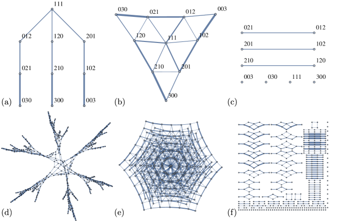
Figure 1: Connectivity of the Hilbert space. Adjacency graph for (a) $H_{1}$, (b) $H_{2}$, (c) $H_{3}$, all for $L=N_{\mathrm{p}}=3$. (d), (e) and (f): same as (a), (b) and (c) but for $L=N_{\mathrm{p}}=6$. To avoid clutter, we do not label the vertices in (d), (e) and (f). All graphs are weighted, i.e., the line thickness is proportional to the magnitude of the corresponding hopping coefficient. Several different clusters of configurations are visible in the case of $H_{1}$. The clusters start to form already for $L=3$ (for example, the configurations $012$-$021$-$003$ in (a)) and become more prominent for $L=6$ (d). In the case of $H_{2}$, almost all configurations are well-connected to the rest of the graph. The graphs for $H_{3}$ show that the Hilbert space is highly reducible: its graph splits into many disconnected components.

I Results

I.1 Models and their Hilbert spaces

A fundamental ingredient of kinetically constrained models is “correlated hopping”: a particle can hop depending on the state of its neighbors. In this paper we consider a system of $N_{\mathrm{p}}$ bosons on a one-dimensional lattice with $L$ sites. We consider models where the total filling factor, $\nu=N_{\mathrm{p}}/L$, is conserved, and we will mainly present results in the dense regime, $\nu=1$. We have studied models with $\nu<1$ and $\nu>1$, but we found them to be either too constrained or not constrained enough, and therefore less interesting. We emphasize that the bosons in our study are not hard-core, i.e., the occupancy of any lattice site can take any value from $0$ to $N_{\mathrm{p}}$.

We study three different models, defined by the Hamiltonians:

$$H_{1} = -J\sum_{j=1}^{L}\left(b^{\dagger}_{j}b_{j+1}n_{j}+n_{j-1}b^{\dagger}_{j}b_{j-1}\right),$$ (1)

$$H_{2} = -J\sum_{j=1}^{L}\left(n_{j}b^{\dagger}_{j}b_{j+1}+b^{\dagger}_{j}b_{j-1}n_{j-1}\right),$$ (2)

$$H_{3} = -J\sum_{j=1}^{L}\left(n_{j+1}b^{\dagger}_{j}b_{j+1}n_{j}+n_{j-1}b^{\dagger}_{j}b_{j-1}n_{j}\right).$$ (3)

All three models contain a free-boson hopping term, $b_{j}^{\dagger}b_{j+1}$, which is dressed in various ways by density operators, $n_{j}=b^{\dagger}_{j}b_{j}$. We will show that the position of the density operator $n_{j}$ completely changes the behavior of these models, ranging from fast thermalization to the breakup of the Hamiltonian into disconnected, exactly solvable sectors. For example, note that $H_{1}$ and $H_{2}$ are related to each other via free boson hopping,

$$H_{2} = H_{1}-J\sum_{j}\left(b^{\dagger}_{j}b_{j+1}+b^{\dagger}_{j}b_{j-1}\right),$$ (4)

which can be easily proven using bosonic commutation relations. We will see below that this innocuous free-boson hopping leads to surprisingly different dynamical properties of the two models.

The motivation behind introducing three different models in Eqs. (1)-(3) can be summarized as follows. Hamiltonian $H_{1}$ describes a model where a particle cannot hop to the left if that site is not already occupied by at least one particle, and cannot hop to the right if it is the only particle left on its initial site. This introduces constraints to the system. Conversely, there are no such constraints in the case of $H_{2}$. Indeed, the hopping coefficients are only modified in intensity by the particle-number operator. Hamiltonian $H_{3}$ introduces additional constraints compared to $H_{1}$. The number of unoccupied sites and their positions remain constant under the action of this Hamiltonian. This leads to different connectivity of the Hilbert space in each of the models, as we explain in the next Section.

We consider periodic boundary conditions ($L+1\equiv 1$) and set $\hbar=J=1$. With periodic boundary conditions, all three Hamiltonians $H_{1}$, $H_{2}$ and $H_{3}$ have translation symmetry, thus their eigenstates can be labelled by momentum quantum number, $k$, quantized in units of $2\pi/L$. In addition, $H_{3}$ has inversion symmetry. We denote by $I=0$ and $I=1$ the sectors that are even and odd under inversion, respectively.

Without restrictions on the boson occupancy, the Hilbert space of $H_{1}$, $H_{2}$ and $H_{3}$ grows very rapidly. For $L=N_{\mathrm{p}}=12$, the Hilbert space size of the $k=0$ sector is $112720$ (the largest one we will consider for $H_{1}$ and $H_{2}$). As previously mentioned (see also the next Section), the Hilbert space of $H_{3}$ splits into many disconnected components, thus it is possible to consider only one connected component at a time and disregard the unoccupied sites whose positions do not change. This is more relevant when looking at properties such as thermalization, than fixing the filling factor. However, the boundary conditions are in that case no longer periodic, and the system does not have translation symmetry. Considering only a system with the size $L/2$, filling factor $\nu=2$, open boundary conditions and minimal number of particles per site equal to $1$ is completely equivalent to considering the largest component of the full system which has the size $L$, filling factor $\nu=1$, periodic boundary conditions and no restrictions on the occupancies. The Hilbert space size of the symmetric invariant sector of the largest connected component of $L=N_{\mathrm{p}}=22$ is $176484$ and this is the largest sector that we will consider for $H_{3}$.

I.2 Graph structure of the models

Since we will be interested in the dynamical properties, it is convenient to first build some intuition about the structure of the Hamiltonians of the three models in Eqs. (1)-(3). A Hamiltonian can be viewed as the adjancency matrix of a graph whose vertices are Fock states of bosons, $|n_{1},n_{2},\ldots,n_{L}\rangle$. If the Hamiltonian induces a transition between two Fock states, the corresponding vertices of the graph are connected by a link. The graphs that show how the configuration space is connected have very different structure for the three Hamiltonians $H_{1}$, $H_{2}$ and $H_{3}$, as can be observed in Fig. 1.

The entire graph of $H_{2}$ is well-connected and it has the same structure as the graph of the standard Bose-Hubbard model: the particle-number operators in $H_{2}$ do not introduce any constraints, but only affect the magnitude of the hopping coefficients. In contrast, the $H_{1}$ graph shows several clusters of configurations that are weakly connected to the rest of the graph. “Weakly connected” means that there is a small number of connections leading outside the cluster and that their respective hopping coefficients are smaller in magnitude than those of the surrounding connections within the cluster. A state that is initially located inside a cluster is therefore more likely to stay inside during an initial stage of the time evolution, which increases the probability of revivals and slows down the growth of entanglement entropy. We will provide a more quantitative description and examples that illustrate this in Section “Quantum scars in $H_{1}$ and $H_{3}$ models”. Finally, the graph of $H_{3}$, due to even stronger constraints, is actually disconnected, which is an example of Hilbert space fragmentation that was previously shown to cause non-ergodic behavior in fracton-like models Khemani and Nandkishore (2019); Sala et al. (2020). This predicts that thermalization and dynamics in the three models will be very different, which we will confirm in the following Section. However, we note that the number of connections and the topology of the graph is not the only relevant factor for the dynamics. The magnitude of the hopping coefficients between different configurations is also important (Supplementary Note 1).

We note that the relation between $H_{1}$ and $H_{3}$ is reminiscent of the relation between the quantum East model van Horssen et al. (2015b) and the “PXP” model describing the atoms in the Rydberg blockade regime Lesanovsky and Katsura (2012); Turner et al. (2018a, b). Like $H_{3}$, the PXP model is doubly constrained and inversion symmetric, while $H_{1}$ and the quantum East model are asymmetric versions of those two models with only a single constraint. The graph of the quantum East model is similar to that of $H_{1}$, in that it contains bottlenecks which slow down the growth of entanglement entropy van Horssen et al. (2015b).

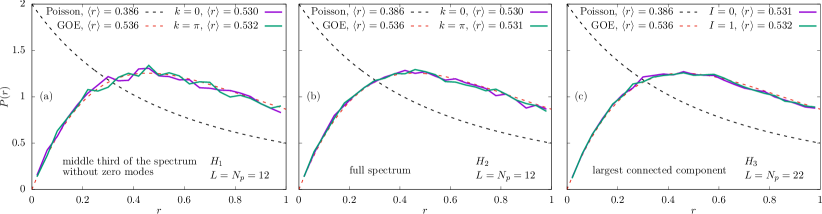
Figure 2: Level statistics and entanglement. (a), (b) and (c): Probability distribution of the ratios of two consecutive energy gaps. (a) $H_{1}$ (middle third of the spectrum without $E=0$ states, $L=N_{\mathrm{p}}=12$), (b) $H_{2}$ (full spectrum, $L=N_{\mathrm{p}}=12$) and (c) $H_{3}$ (largest connected component of $L=N_{\mathrm{p}}=22$). The black dashed line shows the Poisson distribution, which corresponds to the integrable case, while the red dashed line is the distribution of the Gaussian orthogonal ensemble, which corresponds to the thermalizing case. (d), (e) and (f): Entanglement entropies $S_{L/2}$ of all eigenstates plotted as a function of the eigenstate energy per particle, $E/N_{\mathrm{p}}$. (d) $H_{1}$ ($L=N_{\mathrm{p}}=12$, $L_{\mathrm{A}}=6$, $k=0$), (e) $H_{2}$ (same) and (f) $H_{3}$ in the largest connected component of $L=N_{\mathrm{p}}=20$, $L_{\mathrm{A}}=10$, $I=0$. The inset shows all connected components for $L=N_{\mathrm{p}}=12$, $L_{\mathrm{A}}=6$, $k=0$.

I.3 Dynamics and entanglement properties

We now investigate the phenomenology of the models introduced in Eqs. (1)-(3). We use exact diagonalization to obtain the complete set of energy eigenvalues and eigenvectors, from which we evaluate the level statistics and the distribution of entanglement entropies for the three models. Furthermore, we probe dynamical properties of the models by studying a global quench, simulated via Krylov iteration.

The energy level statistics is a standard test for thermalization of models that cannot be solved exactly. A convenient way to probe the level statistics is to examine the probability distribution $P(r)$ Oganesyan and Huse (2007) of ratios between consecutive energy gaps $s_{n}=E_{n+1}-E_{n}$,

$$r=\frac{\mathrm{min}(s_{n},s_{n+1})}{\mathrm{max}(s_{n},s_{n+1})}.$$ (5)

The advantage of studying $P(r)$, instead of $P(s_{n})$, is that there is no need to perform the spectrum unfolding procedure – see Ref. D’Alessio and Rigol, 2014. For standard random matrix theory ensembles, both $P(r)$ and the mean $\langle r\rangle$ are well-known Mehta (2004). When computing the same quantities in a microscopic physical model, it is crucial to resolve all the symmetries of the model.

The probability distribution $P(r)$ of the ratios of two consecutive energy gaps is shown in Figs. 2(a), (b) and (c) for the three Hamiltonians $H_{1}$, $H_{2}$ and $H_{3}$ respectively, and two momentum or inversion sectors. In all three cases, the energy levels repel, i.e., the distribution tends to zero as $r\to 0$. For $H_{2}$, the distribution is particularly close to the Wigner-Dyson (non-integrable) line. For $H_{1}$, the distribution is also consistent with Wigner-Dyson when we restrict to the middle 1/3 of the spectrum (and after removing special states with $E=0$). We exclude the edges of the spectrum because they contain degeneracies which are not symmetry-related. However, such states do not appear to have a major effect on the level statistics distribution, which is still closer to the Wigner-Dyson than the Poisson distribution even if they are included. The level statistics of $H_{3}$ within the largest connected component of the Hilbert space is shown in Fig. 2(c) and is also consistent with the Wigner-Dyson distribution without restricting the spectrum. However, we will demonstrate below that the dynamics in some smaller connected components of $H_{3}$ can be exactly solved.

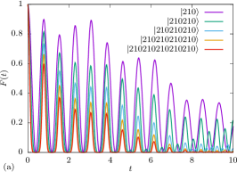
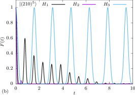
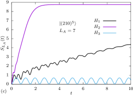
Figure 3: Dynamics of quantum fidelity and entanglement entropy for initial configurations in Eq. (9). (a) Time evolution of fidelity $F(t)$ in Eq. (8) for system sizes $L=3n$. The evolution is governed by the Hamiltonian $H_{1}$, different colors represent different system sizes $L$. (b) Fidelity evolution $F(t)$ for the Hamiltonians $H_{1}$, $H_{2}$ and $H_{3}$ and system size $L=15$. (c) Entanglement entropy evolution $S_{L_{\mathrm{A}}}(t)$ for the same cases as in (b).

As a complementary diagnostic of thermalization, we next compute the entanglement entropy of all eigenstates. We divide the lattice into two sublattices, A and B, of lengths $L_{\mathrm{A}}$ and $L_{\mathrm{B}}=L-L_{\mathrm{A}}$. For a given pure state $|\psi\rangle$, the entanglement entropy is defined as

$$S_{\mathrm{A}}=-\mathrm{tr}_{\mathrm{A}}(\rho_{\mathrm{A}}\ln\rho_{\mathrm{A}}),$$ (6)

where $\rho_{\mathrm{A}}=\mathrm{tr}_{\mathrm{B}}|\psi\rangle\langle\psi|$ is the reduced density matrix of the subsystem A. The scatter plots, showing entanglement entropy of all eigenstates $|E_{n}\rangle$ as a function of their energy $E_{n}$, are displayed in Figs. 2(d), (e) and (f). Here we take into account the translation symmetry of the system and work in the momentum sector $k=0$ for $H_{1}$ and $H_{2}$, and consider only the largest connected component and the inversion sector $I=0$ for $H_{3}$. The results for other sectors are qualitatively similar.

Entanglement entropy distribution in Figs. 2(d) and (e) reveals a striking difference between the Hamiltonians $H_{1}$ and $H_{2}$, even though they only differ by a free-boson hopping term, Eq. (4). The model $H_{1}$ is constrained, which leads to a large spread of the entropy distribution and many low-entropy eigenstates including in the bulk of the spectrum. From this perspective, $H_{1}$ is reminiscent of PXP model Turner et al. (2018b); Khemani et al. (2019). By contrast, $H_{2}$ has no such constraints and in this case the entanglement entropy is approximately a smooth function of the eigenstate energy. The Hamiltonian $H_{3}$ is doubly constrained, and this is reflected in its entanglement distribution, which also shows a large spread and several disconnected bands, reminiscent of an integrable system like the XY model Alba et al. (2009).

I.4 Global quenches

The constraints in the models in Eqs. (1), (2) and (3) have significant effects on the dynamics governed by these Hamiltonians. We probe the dynamics by performing a global quench on the system. We assume the system is isolated and prepared in one of the Fock states, $|\psi_{0}\rangle$, at time $t=0$. We restrict to $|\psi_{0}\rangle$ being product states which are not necessarily translation-invariant, as such states are easier to prepare in experiment. However, our results remain qualitatively the same if we consider translation-invariant $|\psi_{0}\rangle$. After preparing the system in the state $|\psi_{0}\rangle$, which is not an eigenstate of the Hamiltonian, the system is let to evolve under unitary dynamics,

$$|\psi(t)\rangle=\exp\left(-\frac{i}{\hbar}Ht\right)|\psi_{0}\rangle.$$ (7)

where $H$ is one of the Hamiltonians of interest. From the time-evolved state, we evaluate the quantum fidelity,

$$F(t)=|\langle\psi_{0}|\psi(t)\rangle|^{2},$$ (8)

i.e., the probability for the wave function to return to the initial state. In a general many-body system, fidelity is expected to decay as $F(t)\sim\exp(-L(Jt)^{2})$. It thus becomes exponentially suppressed in the system size for any fixed time $t^{*}$, i.e., $F(t^{*})\sim\exp(-cL)$, where $c$ is a constant. In scarred models, such as the Rydberg atom chain, fidelity at the first revival peak occurring at a time $T$ still decays exponentially, but exponentially slower, i.e., $F(T)\sim\exp(-c^{\prime}L)$, with $c^{\prime}\ll c$. In Ref. Turner et al., 2018b, for a finite system with $L\lesssim 32$ atoms, the fidelity at the first revival can be as high as $\sim 70\%$, and several additional peaks at times $nT$ are also clearly visible.

We first consider the Hamiltonian $H_{1}$. Several configurations exhibit periodic revivals of the fidelity $F(t)$, which can in some cases be higher than $90\%$. Most of these configurations involve a very dense cluster of bosons such as $\lvert...0N10...\rangle$. In contrast, a completely uniform configuration $\lvert...111...\rangle$ thermalizes very quickly. Here we focus on periodically-reviving configurations with density being as uniform as possible. One family of such reviving configurations involves $n$ unit cells made of 3 lattice sites:

$$|210210\ldots 210\rangle\equiv|(210)^{n}\rangle.$$ (9)

Time evolution of the fidelity for the initial state $|(210)^{n}\rangle$ for different system sizes $L=3n$ is shown in Fig. 3(a). The initial state is assumed to be the product state, e.g., $\lvert\psi_{0}\rangle=|210\rangle$ for $L=3$. The frequency of the revivals in Fig. 3 is approximately the same for all system sizes. We emphasize that similar results are obtained for a translation-symmetric initial state, e.g., $\lvert\psi_{0}\rangle=\frac{1}{\sqrt{3}}\left(\lvert 210\rangle+\lvert 021\rangle+\lvert 102\rangle\right)$. Both cases converge in the large system limit, and the differences are only significant for $L=3$ when the revival frequency of the initial state with transition symmetry differs from the frequencies of other system sizes.

In Fig. 3(b) we compare the fidelity for the initial state in Eq. (9) when it is evolved by all three Hamiltonians in Eqs. (1)-(3). The initial state is fixed to be $\lvert(210)^{5}\rangle$. We observe that the dynamics with $H_{3}$ has very prominent revivals; in fact as we will later show, these revivals are perfect and their period is approximately twice the revival period for $H_{1}$. In contrast, for $H_{2}$ the fidelity quickly drops to zero without any subsequent revivals.

Finally, in Fig. 3(c) we plot the time evolution of entanglement entropy. As expected from the fast decay of the fidelity, the entropy for $H_{2}$ rapidly saturates to its maximal value. Moreover, as expected from the perfect revivals in $H_{3}$, the entropy in that case oscillates around a constant value close to zero. For $H_{1}$, we observe a relatively slow growth of entropy, with oscillations superposed on top of that growth, again similar to PXP model Turner et al. (2018a). For the initial state that is not translation-invariant, it is important how we cut the system, e.g., $|...210|210...\rangle$ versus $|...2102|10...\rangle$. In the first case, the entanglement entropy remains zero for $H_{3}$ because no particle can hop from one subsystem to the other, while in the second case the entropy oscillates around a constant value, which is the case in Fig. 3(c).

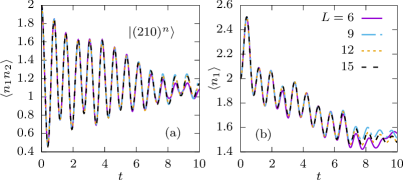
Figure 4: Evolution of local observables for the Hamiltonian $H_{1}$. (a) Correlations between adjacent sites $\langle n_{1}n_{2}(t)\rangle$ for different system sizes and the initial state $|(210)^{n}\rangle$. (b) Density on one site $\langle n_{1}(t)\rangle$.

In Fig. 4 we show the $H_{1}$ evolution of two local observables, density correlations between two adjacent sites $\langle n_{1}n_{2}(t)\rangle$ and density on the first site $\langle n_{1}(t)\rangle$, starting from the initial state $|(210)^{n}\rangle$. Unlike fidelity and entanglement entropy, these observables can be easily measured in experiment. Both observables robustly oscillate with approximately the same frequency as the fidelity. The heights of the first few revival peaks are approximately converged for the system sizes ranging from $L=6$ to $L=15$, which suggests that revivals in such local observables can be observed in the thermodynamic limit. In the following Section, we will show that the oscillations observed in the dynamics from $|(210)^{n}\rangle$ state in Eq. (9) and their frequency can be explained using a tractable model that involves only a small subset of all configurations in the Hilbert space, thus providing a realization of quantum scars in a correlated bosonic system. Our starting point will be the model $H_{3}$, whose graph explicitly separates into disconnected subsets which makes the toy model exact, hence we can analytically calculate the revival frequency. Based on these results, we then introduce an approximation scheme that describes the dynamics from the same initial state under the $H_{1}$ Hamiltonian.

I.5 Quantum scars in $H_{1}$ and $H_{3}$ models

The quench dynamics of fidelity and entanglement entropy in Fig. 3 suggest that $H_{1}$ and $H_{3}$ models are candidate hosts for many-body scarred eigenstates that can be probed by initializing the system in product states $|(210)^{n}\rangle$. We now analyze the structure of these states using our approach called “cluster approximation” that is introduced in detail in Methods.

The dynamics of $H_{3}$ within the sector containing the state $\lvert(210)^{n}\rangle$ can be solved exactly, as shown in Methods. The connected component of the state $\lvert(210)^{n}\rangle$ consists of all possible combinations of patterns $210$ and $120$. This means that triplets of sites evolve independently, and dynamically the system behaves as a collection of independent two level systems (spins-1/2). From this observation, it can be shown that revivals will be perfect with a period $T_{3}=\pi/2$. The same period is obtained for initial product state $\lvert(210)^{n}\rangle$ and its translation-invariant version; if the initial state is both translation-invariant and inversion-symmetric, the period is doubled.

In contrast to the free dynamics in $H_{3}$, the $H_{1}$ model exhibits decaying revivals and does not admit an exact description. In order to approximate the quench dynamics and scarred eigenstates in $H_{1}$, we project the Hamiltonian to smaller subspaces of the full Hilbert space. These subspaces contain clusters of states which are poorly connected to the rest of the Hilbert space and thereby cause dynamical bottlenecks. As explained in Methods, the clusters can be progressively expanded to yield an increasingly accurate description of the dynamics from a given initial state.

For our initial state $|(210)^{n}\rangle$, the minimal cluster is defined as one that contains all the states given by tensor products of $210$, $120$ and $300$ patterns. Similar to the $H_{3}$ case, within this approximation, triplets of sites again evolve independently, and the dimension of the reduced Hilbert space is $\mathrm{dim}\mathcal{H}^{\mathrm{c}}=3^{L/3}$. The time-evolved state within the cluster is given by

$$\lvert\psi^{\mathrm{c}}_{n}(t)\rangle=\cos^{n}(4t)\lvert(210)^{n}\rangle+\ldots,$$ (10)

where the dots denote other configurations. The fidelity is

$$F^{\mathrm{c}}_{n}(t)=\lvert\langle\psi^{\mathrm{c}}_{n}(0)\lvert\psi^{\mathrm{c}}_{n}(t)\rangle\lvert^{2}=\lvert\cos(4t)\lvert^{2n}.$$ (11)

As in the case of $H_{3}$, this result is also valid for the translation-invariant initial state. We see that the period of revivals is $T_{1}=\pi/4$, which is the same as for $H_{3}$ with a translation and inversion symmetric initial state.

The result of the cluster approximation is compared against the exact result for system size $L=15$ in Fig. 5. The frequency of the fidelity revival, shown by the blue line in Fig. 5(a), is accurately reproduced in this approximation, however the approximation does not capture the reduction in the magnitude of $F(t)$. Similarly, the dynamics of entanglement entropy, blue line in Fig. 5(b), is only captured at very short times. In particular, we observe that the maximum entanglement within the cluster remains bounded even at long times $t\sim 10$, while the exact entropy continues to increase and reaches values that are several times larger.

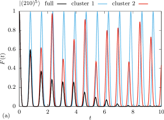
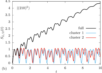
Figure 5: Comparison of the full dynamics against the minimal cluster ($1$) and extended cluster ($2$) approximation schemes. We consider the system size $L=15$ with the initial state $\lvert(210)^{5}\rangle$. (a) Time evolution of the fidelity. The frequency of revivals is approximately the same in both cases, but the results for the extended cluster show better agreement with the results for the full Hilbert space. (b) Time evolution of the entanglement entropy.

To obtain a more accurate approximation, we can expand the minimal cluster with several neighboring configurations on the graph. We define the extended cluster as a set of all states which can be obtained using tensor products of the configurations $210$, $120$, $300$ and $111$. The enlarged cluster clearly contains the minimal cluster studied above, but it also includes additional configurations, resulting in a much better prediction for the first revival peak height, while still allowing for analytical treatment. The dimension of the extended cluster grows as $\mathrm{dim}\mathcal{H}^{\tilde{\mathrm{c}}}=4^{L/3}$, and is thus exponentially larger than the minimal cluster approximation. Nevertheless, the extended cluster dimension is still exponentially smaller compared to the full Hilbert space, and within this approximation it is possible to numerically simulate the dynamics of larger systems, $L\lesssim 30$ – see Fig. 6(a). The revivals are no longer perfect, while their frequency is independent of the system size and closer to the frequency of revivals for the full Hilbert space compared to to the minimal cluster approximation in Fig. 5. The overlap between the eigenstates of the Hamiltonian $H_{1}$ reduced to both the minimal and extended cluster and the state $\lvert(210)^{8}\rangle$ is given in Fig. 6(b). The eigenstates that correspond to the minimal cluster approximately survive in the extended cluster, where they form a band with the highest overlap.

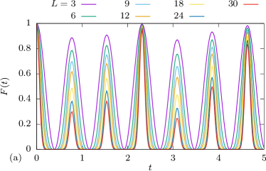
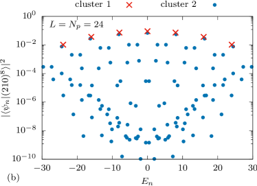
Figure 6: Cluster approximations. (a) Fidelity $F(t)$, for the Hamiltonian $H_{1}$ and initial states $\lvert(210)^{n}\rangle$, in the extended cluster approximation for various system sizes. (b) Eigenstate overlap with the initial state $\lvert(210)^{8}\rangle$ plotted on a log scale, for both cluster approximations. In the case of degenerate eigenstates the sum of their overlaps is shown.

For the initial product state $(210)^{n}$, it is possible to analytically obtain the fidelity within the improved approximation for arbitrary system size. Similar to the previous methods, it can be shown (see Supplementary Note 2)

$$F^{\tilde{\mathrm{c}}}_{L=3n}(t) = 4^{n}\lvert b^{2}\cos(\alpha t)+d^{2}\cos(\beta t)\lvert^{2n},$$ (12)

where $\alpha=\sqrt{9+\sqrt{57}}\approx 4.06815$, $\beta=\sqrt{9-\sqrt{57}}\approx 1.20423$, $b\approx 0.694113$ and $d\approx 0.134933$. Eq. (12) is in excellent agreement with the numerical results in Fig. 6(a). It was also found to be a very good approximation for the translation-invariant initial state when $L\geq 9$ (data not shown).

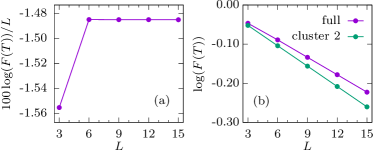
Figure 7: First peak height. (a) Logarithm (base 10) of the first revival peak divided by the system size, $\log(F(T))/L$, seems to saturate at a finite value in the thermodynamic limit. (b) Comparison of the logarithm of the first revival peak height for the full dynamics and the improved cluster approximation. The approximation serves as a lower bound.

Fig. 7(a) shows that the logarithm of the fidelity per site, $\log(F(T))/L$, at the first peak, saturates at a finite value for large $L$. In the improved cluster approximation, the first peak height decays as $\mathrm{e}^{-0.04L}$ (Supplementary Note 2). For a completely random state, the fidelity would be $F\sim 1/{\mathrm{dim}_{\mathcal{H}}}$. In the case $\nu=1$ and large $L$, the Hilbert space dimension grows with the system size as

$$\mathrm{dim}_{\mathcal{H}}={{2L-1}\choose{L}}\approx{{2L}\choose{L}}\approx\frac{4^{L}}{\sqrt{\pi L}}.$$ (13)

This back-of-the-envelope estimate suggests the fidelity of a random state is $F\sim\mathrm{e}^{-1.39L}$, which decays considerably faster than the first peak height in Fig. 7. The improved cluster approximation correctly reproduces the short-time dynamics, including the first revival peak, and sets a lower bound for the first peak height – see Figs. 5 and 7(b).

Figure 8: Evolution of the probability to remain inside the minimal cluster. $\mathcal{O}_{\mathrm{Cluster}}$, as defined in Eq. (14). Initial configurations are indicated in the legend. Solid lines: configurations initially inside the cluster. Dashed lines: configurations initially outside the cluster (all except $\lvert(111)^{4}\rangle$ are randomly chosen). Similar results are obtained for the extended cluster (not shown). System size $L=12$.

The evolution of the entanglement entropy for the extended cluster approximation is shown in Fig. 5(b). Inside the cluster, entropy remains approximately constant with periodic oscillations that have the same frequency as the wave function revivals. Any further growth of the entanglement entropy can be attributed to the spreading of the wave-function outside the cluster. To illustrate the “leakage” of the wave function outside the cluster, in Fig. 8 we compute the time evolution of the overlap with a cluster, i.e., the probability to remain inside a cluster at time $t$,

$$\mathcal{O}_{\mathrm{Cluster}}=\sum_{a\in\mathrm{Cluster}}|\langle a|\psi(t)\rangle|^{2}.$$ (14)

We consider several initial configurations that lie inside or outside the cluster. The configurations initially inside the cluster mostly stay there, and the configuration $\lvert(210)^{4}\rangle$ that has the highest revivals also has the highest overlap. Similarly, configurations initially outside the cluster continue to have negligible overlaps. The overlap starting from the configuration $\lvert(210)^{4}\rangle$ approximately predicts the revival peak heights for the full dynamics.

We now summarize the relation between $H_{3}$ and $H_{1}$ from the point of view of the cluster approximation. For the initial state $\lvert(210)^{n}\rangle$, the two models yield similar dynamics, compare Eqs. (23) and Eq. (12). The only difference is that the revival frequency is doubled in the latter case, which can be easily explained by the symmetry of the initial state and that of the Hamiltonian. Hamiltonian $H_{3}$ is inversion-symmetric. If the initial state is also chosen to be inversion-symmetric, the frequency of the revivals doubles. The period is then $T_{3}^{\mathrm{inv}}=\pi/4$, which is equal to the period of revivals $T_{1}$ of $H_{1}$ in the cluster approximation. This is also proven analytically in Methods, see Eq. (27). For comparison, the revival period for the full Hilbert space is approximately $0.77$, which is slightly less than $\pi/4\approx 0.79$. The Hamiltonian $H_{1}$ is not inversion-symmetric, so the frequency does not double for an inversion-symmetric initial state, but the revivals are lower in that case. This shows that it is important for the symmetry of the initial state to match the symmetry of the Hamiltonian.

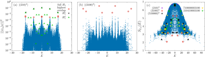
Figure 9: Non-ergodic eigenstates. (a) Overlap of the configuration $\lvert(210)^{4}\rangle$ with all the eigenstates of $H_{1}$, $H_{1}^{c}$ and $H_{1}^{\tilde{c}}$ versus the eigenstate energy for sector $k=0$ and system size $L=N_{p}=12$. (b) Same for $\lvert(3100)^{3}\rangle$. (c) Entanglement entropy, eigenstates which have the highest overlap with some product states are marked in different colors.

Finally, the eigenstates of $H_{1}$, projected to the subspace of the minimal cluster approximation, form several degenerate bands whose eigenenergies are equally spaced in integer multiples of $4$. Interestingly, some of these eigenstates approximately survive in the full $H_{1}$ model, and they are precisely the eigenstates that have the highest overlap with the configurations $\lvert(210)^{n}\rangle$, see Fig. 9(a). In small system sizes, such as $L=6$, the surviving eigenstates are also the lowest entropy eigenstates in the middle of the spectrum, which is reminiscent of quantum scars in the PXP model Turner et al. (2018b). In larger systems, e.g., $L=12$, the surviving eigenstates are slightly lower in entropy than their neighbors, but are far from being the lowest entropy eigenstates, as can be seen in Fig. 9. The lowest entropy eigenstates have high overlaps with other configurations, such as $\lvert(3100)^{3}\rangle$, as shown in Figs. 9(b) and 9(c). In the case of $\lvert(210)^{n}\rangle$, the eigenstates surviving in the full system belong to every other band of eigenstates in the cluster approximation and the number of the surviving eigenstates is $n+1$. For even system sizes this counting includes a zero-energy eigenstate. In Methods we discuss in more details the generalization of the cluster approximations to the states of the form $\lvert(N10...0)^{n}\rangle$, which were also found to have robust revivals and high overlaps with some low-entropy eigenstates.

II Discussion

In this paper, we have introduced three models of bosons with “soft” kinetic constraints, i.e., density-dependent hopping. We have demonstrated that some of these models exhibit similar phenomenology to other realizations of quantum many-body scars, for example the Rydberg atom system Bernien et al. (2017). We have studied quantum dynamics of these systems by performing global quenches from tensor-product initial states. We have shown that both the connectivity of the Hilbert space and the relative magnitude of the hopping coefficients have dramatic effects on the dynamics. For certain initial configurations, the constraints can lead to slow thermalization and revivals in the quantum fidelity. The revival frequency can be predicted by considering an exponentially reduced subset of the Hilbert space. For a family of initial configurations of the form $\lvert(210)^{n}\rangle$, we have derived analytical expressions for the evolution of quantum fidelity within this approximation, which accurately capture the revival frequency obtained from exact numerical data. One notable difference between scarred dynamics in the present bosonic models and the PXP model is that the revivals exist in the absence of a hard kinetic constraint, i.e., in the fully connected Hilbert space. Our cluster approximation also explains the structure of some low-entropy eigenstates in the middle of the many-body spectrum. In addition, we have calculated the evolution of two local observables which are experimentally measurable, density correlations between two neighboring sites and density on a single site, and both of them show robust oscillations over a range of system sizes. We have also shown that the introduced models contain additional special properties, like the exponentially large zero-energy degeneracy which is related to the bipartite structure of the model.

We now comment on the possible experimental realizations of the models we studied. The implementation of a correlated hopping term ($n_{k}b_{i}^{\dagger}b_{j}$) in optical lattices has attracted lot of attention due to a possible onset of quantum phases related to high-Tc superconductivity Eckholt and García-Ripoll (2009). An early theoretical proposal exploits asymmetric interactions between the two atomic states in the presence of a state-dependent optical lattice Eckholt and García-Ripoll (2009). As a result, the obtained effective model corresponds to the inversion-symmetric form of $H_{1}$. In addition, the same term has been found to feature as a higher-order correction of the standard Bose-Hubbard model Mazzarella et al. (2006); Bissbort et al. (2012); Lühmann et al. (2012); Dutta et al. (2015). Although in this case the term typically represents a modification of the regular hopping term of the order of several percent, its contribution was directly measured Jürgensen et al. (2014); Baier et al. (2016). More recently, the set of quantum models accessible in cold-atom experiments has been enriched through the technique of Floquet engineering Eckardt (2017). As a notable example, a suitable driving scheme can renormalize or fully suppress the bare tunneling rate Eckardt et al. (2009). On top of that, by modulating local interactions an effective model with the density-dependent tunneling term has been engineered Meinert et al. (2016). For the models considered in this paper the most promising is a more recent driving scheme exploiting a double modulation of a local potential and on-site interactions Zhao et al. (2019). Related sophisticated driving schemes have already enabled a realization of dynamical gauge fields Görg et al. (2019); Barbiero et al. (2019); Schweizer et al. (2019) where both the amplitude and the phase of the effective tunneling are density-dependent. Although these experimental proposals explain how to realize some of the correlated hopping terms present in our models using ultracold atoms in optical lattices, finding a scheme that exactly realizes our models requires further study. We emphasize that other models which would exhibit non-ergodic dynamics and scarred eigenstates as a result of the same mechanism that was explained in this work could be built, for example a linear combination of $H_{1}$ and $H_{2}$.

Note added: During the completion of this work, we became aware of Ref. Pancotti et al., 2019 which identified non-thermal eigenstates and slow dynamics in the quantum East model. Moreover, a recent study Zhao et al. (2020) proposed a Floquet scheme for a bosonic model with density-assisted hopping, finding signatures of quantum many-body scars.

III Methods

In order to more efficiently describe the dynamics of our models, we introduce a method – “cluster approximation”, that is based on Hilbert space truncation inspired by the bipartite graph structure of $H_{1}$. Before providing details about the cluster approximation for $H_{1}$ and its generalizations, we present an exact solution for the perfect revivals in $H_{3}$ model, which serves as a motivation for the more complicated case of $H_{1}$.

III.1 Bipartite lattice and zero modes

The graph of $H_{1}$ is bipartite, i.e. all the basis configurations can be divided into two disjoint sets, and the action of the Hamiltonian connects configurations in one set only to the configurations in the other and vice-versa (the Hamiltonian is off-diagonal). One way to sort configurations into these two sets is by parity of the quantity

$$\Delta_{a}=\frac{\lvert n_{\mathrm{even}}-n_{\mathrm{odd}}+C\rvert}{2},$$ (15)

where $C=0$ if $L$ is even and $C=1$ if $L$ is odd. We define $n_{\mathrm{even}}$ and $n_{\mathrm{odd}}$ as the total numbers of particles at even and odd sites, respectively,

$$n_{\mathrm{even}}=\sum_{l=1}^{L_{1}}n_{2l},\ n_{\mathrm{odd}}=\sum_{l=1}^{L_{2}}n_{2l-1},$$ (16)

where $L_{1}=L_{2}=L/2$ if $L$ is even, and $L_{1}=(L-1)/2$, $L_{2}=(L+1)/2$ if $L$ is odd. If only nearest neighbor hoppings are allowed and if no two odd sites are coupled (if the system has open boundary conditions for any $L$ or periodic boundary conditions for $L$-even), each hopping either increases $n_{\mathrm{even}}$ by one and decreases $n_{\mathrm{odd}}$ by one, or vice-versa. This means that each hopping can change $\Delta_{a}$ only by $\pm 1$.

In special cases, like $H_{1}$ at filling factor $\nu=1$, it is also possible to define quantities like $\Delta_{a}$ for odd system sizes and periodic boundary conditions. This is a consequence of the constraints imposed by $H_{1}$, i.e., the fact that a particle cannot hop to an empty site to its left (Supplementary Note 3). Note that $H_{2}$ in the same geometry is not bipartite.

Another way to sort configurations into two sets is by parity of the distance from the configuration $\lvert 111...111\rangle$, which we define as

$$d_{a}=\mathrm{min}_{n}\{\langle 111...111\lvert H_{1}^{n}\lvert a\rangle\neq 0\}.$$ (17)

In this case, the two sets are the configurations with even and with odd distances $d_{a}$. One hopping can change $d_{a}$ only by $\pm 1$ or $0$. Changes by other values are not possible by definition if the Hamiltonian is Hermitian (all hoppings are reversible). Both $d_{a}$ and $\Delta_{a}$ have the same parity, thus $d_{a}$ must always change after one hopping in even system sizes or in systems with open boundary conditions. As a consequence, $d_{a}$ cannot change by $0$ if $\Delta_{a}$ can only change by $\pm 1$.

The graphs of bipartite systems do not contain any loops of odd dimension (triangles, pentagons, heptagons and so on). Moreover, the energy spectra of bipartite systems are symmetric around zero. Their Hamiltonians anticommute with the operator $(-1)^{\Delta_{a}}$. The presence of such an operator in a bipartite lattice leads to exact zero energy states in the spectrum Sutherland (1986); Inui et al. (1994). It can be shown that the exponentially growing number of zero modes of $H_{1}$ is related to the difference between the numbers of elements in the two sets of its bipartite graph (Supplementary Note 4). Additionally, the algebraic structure of zero energy eigenstates can be explained by the structure of the graph – such eigenstates can be constructed as superpositions of configurations from only one of the sets. Similar properties are found for $H_{2}$ for even $L$, as its graph is also bipartite in that case. The properties of the zero-energy manifold are discussed in more detail in Supplementary Note 4.

III.2 Perfect revivals in the $H_{3}$ model

We start with a warmup calculation for $H_{3}$ acting on $L=3$ sites. The connected subspace of $210$ contains only two configurations, $120$ and $210$. The Hamiltonian reduced to this subspace is

$$H^{{}^{\prime}}_{3}=-\begin{pmatrix}0&2\\ 2&0\end{pmatrix},$$ (18)

where the basis vectors are

$$\begin{pmatrix}1\\ 0\end{pmatrix}=\lvert 210\rangle,\ \begin{pmatrix}0\\ 1\end{pmatrix}=\lvert 120\rangle.$$ (19)

The eigenvalues of $H_{3}^{{}^{\prime}}$ are $E_{1}=-2$ and $E_{2}=2$. The initial state $\lvert\psi_{1}(t=0)\rangle=\lvert 210\rangle$ evolves as

$$\lvert\psi_{1}(t)\rangle=\cos(2t)\lvert 210\rangle-i\sin(2t)\lvert 120\rangle,$$ (20)

and the state $\lvert\psi_{2}(t=0)\rangle=\lvert 120\rangle$ evolves as

$$\lvert\psi_{2}(t)\rangle=-i\sin(2t)\lvert 210\rangle+\cos(2t)\lvert 120\rangle.$$ (21)

Previous results can be straightforwardly generalized to larger systems. Let the length of the system be $L=3n$ for simplicity. The connected component of the state $\lvert(210)^{n}\rangle$ consists only of combinations of patterns $210$ and $120$, which means that triplets of sites evolve independently. From Eq. (20), the initial state $\lvert\psi_{n}(t=0)\rangle=\lvert(210)^{n}\rangle$ evolves as

$$\lvert\psi_{L=3n}(t)\rangle = \cos^{n}(2t)\lvert(210)^{n}\rangle$$ (22)

$$+ (-i)^{n}\sin^{n}(2t)\lvert(120)^{n}\rangle+...$$

where “$...$” denotes contributions of the basis configurations other than $\lvert(210)^{n}\rangle$ or $\lvert(120)^{n}\rangle$. The fidelity is

$$F_{L=3n}(t)=\lvert\langle\psi_{n}(0)\lvert\psi_{n}(t)\rangle\lvert^{2}=\lvert\cos 2t\lvert^{2n}.$$ (23)

It follows that the revivals are perfect, with a period $T_{3}=\pi/2$. This result is also valid for the translation-invariant initial state $\lvert(210)^{n}\rangle_{\mathrm{T}}$,

$$\lvert(210)^{n}\rangle_{\mathrm{T}}\equiv\frac{1}{\sqrt{3}}\left(\lvert(210)^{n}\rangle+\lvert(021)^{n}\rangle+\lvert(102)^{n}\rangle\right),\quad\quad$$ (24)

as the connected subspaces of $210$, $021$ and $102$ do not overlap and therefore evolve independently.

However, an initial state that is both translation symmetric and inversion symmetric has different dynamics. The inverse of the configuration $\lvert(210)^{n}\rangle$ is the configuration $\lvert(012)^{n}\rangle$, which is a translation of the state $\lvert(120)^{n}\rangle$ that belongs to the connected subspace of $\lvert(210)^{n}\rangle$. The initial state

$$\lvert\psi^{\mathrm{inv}}_{n}(t=0)\rangle=\frac{1}{\sqrt{2}}\lvert(210)^{n}\rangle_{\mathrm{T}}+\frac{1}{\sqrt{2}}\lvert(120)^{n}\rangle_{\mathrm{T}}$$ (25)

evolves as

$$\lvert\psi^{\mathrm{inv}}_{n}(t)\rangle=\left(\cos^{n}2t+(-i)^{n}\sin^{n}2t\right)\lvert\psi^{\mathrm{inv}}_{n}(t=0)\rangle+...\quad\quad$$ (26)

and the fidelity is

$$F^{\mathrm{inv}}_{n}(t) = \lvert\langle\psi^{\mathrm{inv}}_{n}(0)\lvert\psi^{\mathrm{inv}}_{n}(t)\rangle\lvert^{2}$$ (27)

$$= \lvert\cos^{n}2t+(-i)^{n}\sin^{n}2t\lvert^{2}.$$

The frequency of the revivals is now doubled, so the period is $T^{\mathrm{inv}}_{3}=\pi/4$.

III.3 Cluster approximations for the $H_{1}$ model

Here we introduce a scheme for approximating the dynamics from initial states $(210)^{n}$ in the $H_{1}$ model. As can be observed in Fig. 3, the revival periods are approximately the same for different system sizes. We first focus on the non-trivial case $L=6$. Fig. 10 shows part of the graph that contains the initial state, $\lvert 210210\rangle$. Configurations labelled inside the ellipses denote representatives of an orbit of translation symmetry, i.e., the configurations are translation-invariant such as the one in Eq. (24).

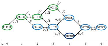
Figure 10: Minimal and extended clusters. Hamiltonian $H_{1}$ and system size $L=N_{\mathrm{p}}=6$. Configurations labelled inside the ellipses are representatives of an orbit of translation symmetry. The minimal cluster is defined by the blue configurations, while green configurations represent the additional components of the extended cluster. Grey arrows connect to configurations outside the extended cluster. The numbers bellow the graph show the distance $d_{a}$ from the configuration $111111$ evaluated using Eq. (17).

The minimal subcluster of the graph is highlighted in blue color in Fig. 10. This cluster is indeed weakly connected to the rest of the configuration space, as it has only $3$ connections that lead outside this cluster (dashed lines) and their hopping coefficients are slightly lower in magnitude than those inside the cluster, meaning that the probability is higher to stay inside the cluster than to leave. The hopping coefficients leading outside are not significantly smaller than the coefficients staying inside, but in combination with the relatively small number of connections this has significant effects on the dynamics. This effect is even more pronounced when the difference in magnitudes is further increased by squaring the particle number operators (see Supplementary Note 1).

The minimal cluster from Fig. 10 contains all the states given by tensor products of $210$, $120$ and $300$ configurations. The set of configurations belonging to this cluster could have been chosen differently, but this particular choice has at least two advantages. Firstly, inside this cluster, the evolution of the configuration $\lvert 210210\rangle$ can be thought of as two subsystems $210$ evolving separately. The evolution of all such configurations at different system sizes can be reduced to the evolution of $L=3$ subsystems $210$, similar to the case of $H_{3}$ in the connected subspace of $(210)^{n}$. Secondly, this definition allows easy generalization to different system sizes $L=3n$ with initial states $(210)^{n}$. We would like to emphasize that the cluster was not chosen arbitrarily. The calculations of the probability density distribution starting from the initial configuration $\lvert 210210\rangle$ and evolving with $H_{1}$ have shown that the probability density stays high in this region of the Hilbert space as long as the revivals in fidelity are visible. The configurations important for the dynamics were then identified by analyzing the structure of the graph around the initial configuration.

As an example, consider system size $L=3$. The reduced Hilbert space of the cluster $\mathcal{H}^{\mathrm{c}}$ is spanned by the (non-translation-invariant) configurations

$$\begin{pmatrix}1\\ 0\\ 0\end{pmatrix}=\lvert 300\rangle,\ \begin{pmatrix}0\\ 1\\ 0\end{pmatrix}=\lvert 210\rangle,\ \begin{pmatrix}0\\ 0\\ 1\end{pmatrix}=\lvert 120\rangle.$$ (28)

The Hamiltonian reduced to this subspace is

$$H_{1}^{\mathrm{c}}=-\begin{pmatrix}0&2\sqrt{3}&0\\ 2\sqrt{3}&0&2\\ 0&2&0\end{pmatrix},$$ (29)

and its eigenvalues are $E_{1}=-4$, $E_{2}=4$, $E_{3}=0$. The initial configuration $\lvert 210\rangle$ evolves according to

$$\lvert\psi^{\mathrm{c}}_{1}(t)\rangle = -\frac{i}{2}\sin(4t)\left(\sqrt{3}\lvert 300\rangle+\lvert 120\rangle\right)$$ (30)

$$+\cos(4t)\lvert 210\rangle.$$

By generalizing this result to larger systems, it is easy to prove Eqs. (10) and (11).

The minimal clusters can be expanded by adding several neighboring configurations. For similar reasons as in the case of minimal clusters, the extended clusters are defined as sets of all states which can be obtained using tensor products of the configurations $210$, $120$, $300$ and $111$. In the case of $L=6$, the enlarged cluster can be observed in Fig. 10. It contains the minimal cluster studied previously, but it also includes additional configurations shown in green ellipses. Again, the approximation could be improved by including more configurations, but this particular choice is well suited for analytical treatment (Supplementary Note 2) and, as shown above, it gives a good prediction for the first revival peak height.

III.4 Generalization to other clusters

Building on the previous observation that some of the low-entropy eigenstates have large weight on $\lvert(3100)^{3}\rangle$ product state, we have investigated periodic revivals from such a larger class of initial states. We find that robust revivals are associated with initial product states of the form

$$\lvert((N-1)1\underbrace{0...0}_{N-2})^{n}\rangle,$$ (31)

where $N$ is the length of the unit cell ($L=Nn$). For example, some of these configurations are $\lvert(3100)^{n}\rangle$, $\lvert(41000)^{n}\rangle$ and $\lvert(510000)^{n}\rangle$. Combinations of those patterns such as $\lvert 310041000\rangle$ also exhibit similar properties, but we will restrict ourselves to the simpler former cases.

We can construct a generalization of the cluster approximation for configurations of the form in Eq. (31). As in the case of $\lvert(210)^{n}\rangle$, the dynamics inside one unit cell explains the dynamics of the full system. The generalized clusters can be chosen in such a way that their Hilbert spaces are spanned by $N$ configurations

$$\lvert i\rangle=\lvert((N+1-i)(i-1)\underbrace{0...0}_{N-2})^{n}\rangle,$$ (32)

where $i$ takes values $1,2,\ldots N$. If we consider only one unit cell ($n=1$), the graph that connects these configurations has a linear structure without any loops, i.e., each configuration $\lvert i\rangle$ is solely connected to the configurations $\lvert i\pm 1\rangle$, except the two configurations at the edges, $\lvert 1\rangle$ and $\lvert N\rangle$, which are only connected to $\lvert 2\rangle$ and $\lvert N-1\rangle$, respectively.

The projection of the Hamiltonian $H_{1}$ to this cluster, which we denote by $H_{1}^{\mathrm{c}}$, has a very simple structure: it has the form of a tight-binding chain with the only nonzero matrix elements on the upper and lower diagonals:

$$H_{1;i,i+1}^{\mathrm{c}}=H_{1;i+1,i}^{\mathrm{c}}=(N-i)\sqrt{i(N+1-i)}.$$ (33)

The dynamics within a single unit cell under $H_{1}^{\mathrm{c}}$ corresponds to density fluctuations between the first and the second site. Following the same procedure as previously, we can now diagonalize $H_{1}^{\mathrm{c}}$ and compute the fidelity time series for the initial configuration $\lvert(N-1)10...0\rangle$. This result can be directly generalized to configurations of the form $\lvert((N-1)10...0)^{n}\rangle$. The derivation is valid for both translation-invariant and non-translation-invariant initial configurations, as the cluster in Eq. (32) is disconnected from its translated copies. We stress that this disconnection, namely the absence of a hopping term between $\lvert 1(N-1)0...0\rangle$ and $\lvert 0N0...0\rangle$, is a consequence of the constraints imposed by $H_{1}$ and it would not hold for $H_{2}$. In this way, we have calculated the time evolution of the fidelity starting from the configurations $\lvert(3100)^{n}\rangle$ (for $n=1,2,3,4$), $\lvert(41000)^{n}\rangle$ ($n=1,2,3$) and $\lvert(510000)^{n}\rangle$ ($n=1,2$), and compared it with the exact numerical results for the full $H_{1}$. The cluster approximation captures both the revival frequency and the height of the first peak. Similar to the $\lvert(210)^{n}\rangle$ case, the approximation can be improved by adding further configurations to the clusters. Moreover, if we want to consider translation-invariant initial states, we can follow the same recipe for $\lvert(210)^{n}\rangle$ by summing translated patterns with the required phase factors given in terms of momenta in multiples of $2\pi/N$. We have checked that revivals appear in these momentum sectors, with roughly the same frequency.

We note that the configurations with larger units cells thermalize more quickly on shorter timescales, but slower at long times. Initially, the states starting from configurations with smaller $N$ have lower entanglement entropies than those with larger $N$. The Hilbert spaces of large $N$ unit cells are larger, so the entanglement entropy starting from these configurations rapidly grows to the maximal value for that unit cell. However, the only way for the wave-function to spread through the entire Hilbert space is that a unit cell reaches a state close to $111...111$, so that particles can hop to the other unit cells. This is less likely for large $N$, and therefore such configurations need long times to fully thermalize. As a result, smaller $N$ entanglement entropies grow faster and after long enough time they overtake those for larger $N$. For example, in the case of $L=12$ and translation-invariant initial states, $(210)^{4}$ overtakes $(3100)^{3}$ and $(510000)^{2}$ around $t\sim 2$, and $(3100)^{3}$ overtakes $(510000)^{2}$ around $t\sim 80$ (Supplementary Fig. 3).

Finally, we note that non-thermal behavior reminiscent of the one studied here was previously observed in an unconstrained Bose-Hubbard model, for example in the context of “arrested expansion” Heidrich-Meisner et al. (2009); Ronzheimer et al. (2013) and quenches from superfluid to Mott insulator phase Greiner et al. (2002); Kollath et al. (2007). In these cases, the main ingredient is the strong on-site interaction, which causes the energy spectrum to split into several bands. Due to the large energy differences between bands, the dynamics of an initial state from a particular band is at first limited only to the eigenstates that belong to the same band. Additionally, these energy bands are approximately equally spaced, which can lead to revivals in fidelity if several bands are populated. In contrast, our models do not feature on-site interaction, and the mechanism which slows down the spread of the wave function is correlated hopping, which suppresses connections between certain configurations and modifies the hopping amplitudes between others, thus creating bottlenecks that separate different clusters of states.

IV Data Availability

The data that support the plots within this paper and other findings of this study are available at https://doi.org/10.5518/810 Hudomal et al. (2020).

V Code Availability

Code is available upon reasonable request.

VI Acknowledgments

The authors thank Thomas Iadecola for fruitful discussions. A.H. and I.V. acknowledge funding provided by the Institute of Physics Belgrade, through the grant by the Ministry of Education, Science, and Technological Development of the Republic of Serbia. N.R. was supported by the Department of Energy Grant No. DE-SC0016239, the National Science Foundation EAGER Grant No. DMR 1643312, Simons Investigator Grant No. 404513, ONR Grant No. N00014-14-1-0330, the Packard Foundation, the Schmidt Fund for Innovative Research, and a Guggenheim Fellowship from the John Simon Guggenheim Memorial Foundation. Z.P. acknowledges support by EPSRC grant EP/R020612/1 and the National Science Foundation under Grant No. NSF PHY-1748958. Part of the numerical simulations were performed on the PARADOX-IV supercomputing facility at the Scientific Computing Laboratory, National Center of Excellence for the Study of Complex Systems, Institute of Physics Belgrade. The authors would also like to acknowledge the contribution of the COST Action CA16221.‌

VII Author contributions

A.H., I.V., N.R. and Z.P. contributed to developing the ideas, analyzing the results and writing the manuscript. A.H. performed the calculations and designed the figures.

VIII Competing interests

The authors declare no competing interests.

References

- Heller (1984) Eric J. Heller, “Bound-state eigenfunctions of classically chaotic Hamiltonian systems: Scars of periodic orbits,” Phys. Rev. Lett. 53, 1515–1518 (1984).
- Sridhar (1991) S. Sridhar, “Experimental observation of scarred eigenfunctions of chaotic microwave cavities,” Phys. Rev. Lett. 67, 785–788 (1991).
- Marcus et al. (1992) C. M. Marcus, A. J. Rimberg, R. M. Westervelt, P. F. Hopkins, and A. C. Gossard, “Conductance fluctuations and chaotic scattering in ballistic microstructures,” Phys. Rev. Lett. 69, 506–509 (1992).
- Wilkinson et al. (1996) P. B. Wilkinson, T. M. Fromhold, L. Eaves, F. W. Sheard, N. Miura, and T. Takamasu, “Observation of scarred wavefunctions in a quantum well with chaotic electron dynamics,” Nature 380, 608–610 (1996).
- Bernien et al. (2017) Hannes Bernien, Sylvain Schwartz, Alexander Keesling, Harry Levine, Ahmed Omran, Hannes Pichler, Soonwon Choi, Alexander S. Zibrov, Manuel Endres, Markus Greiner, Vladan Vuletić, and Mikhail D. Lukin, “Probing many-body dynamics on a 51-atom quantum simulator,” Nature 551, 579–584 (2017).
- Turner et al. (2018a) C. J. Turner, A. A. Michailidis, D. A. Abanin, M. Serbyn, and Z. Papić, “Weak ergodicity breaking from quantum many-body scars,” Nat. Phys. 14, 745–749 (2018a).
- Ho et al. (2019) Wen Wei Ho, Soonwon Choi, Hannes Pichler, and Mikhail D. Lukin, “Periodic orbits, entanglement, and quantum many-body scars in constrained models: Matrix product state approach,” Phys. Rev. Lett. 122, 040603 (2019).
- Schauß et al. (2012) Peter Schauß, Marc Cheneau, Manuel Endres, Takeshi Fukuhara, Sebastian Hild, Ahmed Omran, Thomas Pohl, Christian Gross, Stefan Kuhr, and Immanuel Bloch, “Observation of spatially ordered structures in a two-dimensional Rydberg gas,” Nature 491, 87–91 (2012).
- Labuhn et al. (2016) Henning Labuhn, Daniel Barredo, Sylvain Ravets, Sylvain de Léséleuc, Tommaso Macrì, Thierry Lahaye, and Antoine Browaeys, “Tunable two-dimensional arrays of single Rydberg atoms for realizing quantum Ising models,” Nature 534, 667–670 (2016).
- Calabrese and Cardy (2006) Pasquale Calabrese and John Cardy, “Time dependence of correlation functions following a quantum quench,” Phys. Rev. Lett. 96, 136801 (2006).
- Kinoshita et al. (2006) Toshiya Kinoshita, Trevor Wenger, and David S. Weiss, “A quantum Newton’s cradle,” Nature 440, 900–903 (2006).
- Schreiber et al. (2015) Michael Schreiber, Sean S. Hodgman, Pranjal Bordia, Henrik P. Lüschen, Mark H. Fischer, Ronen Vosk, Ehud Altman, Ulrich Schneider, and Immanuel Bloch, “Observation of many-body localization of interacting fermions in a quasirandom optical lattice,” Science 349, 842–845 (2015).
- Smith et al. (2016) J. Smith, A. Lee, P. Richerme, B. Neyenhuis, P. W. Hess, P. Hauke, M. Heyl, D. A. Huse, and C. Monroe, “Many-body localization in a quantum simulator with programmable random disorder,” Nat. Phys. 12, 907–911 (2016).
- Kucsko et al. (2018) G. Kucsko, S. Choi, J. Choi, P. C. Maurer, H. Zhou, R. Landig, H. Sumiya, S. Onoda, J. Isoya, F. Jelezko, E. Demler, N. Y. Yao, and M. D. Lukin, “Critical thermalization of a disordered dipolar spin system in diamond,” Phys. Rev. Lett. 121, 023601 (2018).
- Kaufman et al. (2016) Adam M. Kaufman, M. Eric Tai, Alexander Lukin, Matthew Rispoli, Robert Schittko, Philipp M. Preiss, and Markus Greiner, “Quantum thermalization through entanglement in an isolated many-body system,” Science 353, 794–800 (2016).
- Choi et al. (2019) Soonwon Choi, Christopher J. Turner, Hannes Pichler, Wen Wei Ho, Alexios A. Michailidis, Zlatko Papić, Maksym Serbyn, Mikhail D. Lukin, and Dmitry A. Abanin, “Emergent SU(2) dynamics and perfect quantum many-body scars,” Phys. Rev. Lett. 122, 220603 (2019).
- Bull et al. (2020) Kieran Bull, Jean-Yves Desaules, and Zlatko Papić, “Quantum scars as embeddings of weakly broken Lie algebra representations,” Phys. Rev. B 101, 165139 (2020).
- Deutsch (1991) J. M. Deutsch, “Quantum statistical mechanics in a closed system,” Phys. Rev. A 43, 2046–2049 (1991).
- Srednicki (1994) Mark Srednicki, “Chaos and quantum thermalization,” Phys. Rev. E 50, 888 (1994).
- Turner et al. (2018b) C. J. Turner, A. A. Michailidis, D. A. Abanin, M. Serbyn, and Z. Papić, “Quantum scarred eigenstates in a Rydberg atom chain: Entanglement, breakdown of thermalization, and stability to perturbations,” Phys. Rev. B 98, 155134 (2018b).
- Iadecola et al. (2019) Thomas Iadecola, Michael Schecter, and Shenglong Xu, “Quantum many-body scars from magnon condensation,” Phys. Rev. B 100, 184312 (2019).
- Moudgalya et al. (2018a) Sanjay Moudgalya, Stephan Rachel, B. Andrei Bernevig, and Nicolas Regnault, “Exact excited states of nonintegrable models,” Phys. Rev. B 98, 235155 (2018a).
- Moudgalya et al. (2018b) Sanjay Moudgalya, Nicolas Regnault, and B. Andrei Bernevig, “Entanglement of exact excited states of Affleck-Kennedy-Lieb-Tasaki models: Exact results, many-body scars, and violation of the strong eigenstate thermalization hypothesis,” Phys. Rev. B 98, 235156 (2018b).
- Lin and Motrunich (2019) Cheng-Ju Lin and Olexei I. Motrunich, “Exact quantum many-body scar states in the Rydberg-blockaded atom chain,” Phys. Rev. Lett. 122, 173401 (2019).
- Khemani et al. (2019) Vedika Khemani, Chris R. Laumann, and Anushya Chandran, “Signatures of integrability in the dynamics of Rydberg-blockaded chains,” Phys. Rev. B 99, 161101 (2019).
- Michailidis et al. (2020) A. A. Michailidis, C. J. Turner, Z. Papić, D. A. Abanin, and M. Serbyn, “Slow quantum thermalization and many-body revivals from mixed phase space,” Phys. Rev. X 10, 011055 (2020).
- Kormos et al. (2016) Marton Kormos, Mario Collura, Gabor Takács, and Pasquale Calabrese, “Real-time confinement following a quantum quench to a non-integrable model,” Nat. Phys. 13, 246–249 (2016).
- James et al. (2019) Andrew J. A. James, Robert M. Konik, and Neil J. Robinson, “Nonthermal states arising from confinement in one and two dimensions,” Phys. Rev. Lett. 122, 130603 (2019).
- Robinson et al. (2019) Neil J. Robinson, Andrew J. A. James, and Robert M. Konik, “Signatures of rare states and thermalization in a theory with confinement,” Phys. Rev. B 99, 195108 (2019).
- Vafek et al. (2017) Oskar Vafek, Nicolas Regnault, and B. Andrei Bernevig, “Entanglement of Exact Excited Eigenstates of the Hubbard Model in Arbitrary Dimension,” SciPost Phys. 3, 043 (2017).
- Iadecola and Žnidarič (2019) Thomas Iadecola and Marko Žnidarič, “Exact localized and ballistic eigenstates in disordered chaotic spin ladders and the Fermi-Hubbard model,” Phys. Rev. Lett. 123, 036403 (2019).
- Haldar et al. (2019) Asmi Haldar, Diptiman Sen, Roderich Moessner, and Arnab Das, “Scars in strongly driven Floquet matter: resonance vs emergent conservation laws,” arXiv e-prints (2019), arXiv:1909.04064 [cond-mat.other] .
- Schecter and Iadecola (2019) Michael Schecter and Thomas Iadecola, “Weak ergodicity breaking and quantum many-body scars in spin-1 magnets,” Phys. Rev. Lett. 123, 147201 (2019).
- Iadecola and Schecter (2020) Thomas Iadecola and Michael Schecter, “Quantum many-body scar states with emergent kinetic constraints and finite-entanglement revivals,” Phys. Rev. B 101, 024306 (2020).
- Moudgalya et al. (2019) Sanjay Moudgalya, B. Andrei Bernevig, and Nicolas Regnault, “Quantum Many-body Scars in a Landau Level on a Thin Torus,” arXiv e-prints (2019), arXiv:1906.05292 [cond-mat.str-el] .
- Pai and Pretko (2019) Shriya Pai and Michael Pretko, “Dynamical scar states in driven fracton systems,” Phys. Rev. Lett. 123, 136401 (2019).
- Khemani and Nandkishore (2019) Vedika Khemani and Rahul Nandkishore, “Local constraints can globally shatter Hilbert space: a new route to quantum information protection,” arXiv e-prints (2019), arXiv:1904.04815 [cond-mat.stat-mech] .
- Sala et al. (2020) Pablo Sala, Tibor Rakovszky, Ruben Verresen, Michael Knap, and Frank Pollmann, “Ergodicity breaking arising from Hilbert space fragmentation in dipole-conserving Hamiltonians,” Phys. Rev. X 10, 011047 (2020).
- Khemani et al. (2019) Vedika Khemani, Michael Hermele, and Rahul M. Nandkishore, “Localization from shattering: higher dimensions and physical realizations,” arXiv e-prints (2019), arXiv:1910.01137 [cond-mat.stat-mech] .
- Shiraishi and Mori (2017) Naoto Shiraishi and Takashi Mori, “Systematic construction of counterexamples to the eigenstate thermalization hypothesis,” Phys. Rev. Lett. 119, 030601 (2017).
- D’Alessio et al. (2016) Luca D’Alessio, Yariv Kafri, Anatoli Polkovnikov, and Marcos Rigol, “From quantum chaos and eigenstate thermalization to statistical mechanics and thermodynamics,” Adv. Phys. 65, 239–362 (2016).
- Gogolin and Eisert (2016) Christian Gogolin and Jens Eisert, “Equilibration, thermalisation, and the emergence of statistical mechanics in closed quantum systems,” Rep. Prog. Phys. 79, 056001 (2016).
- Ok et al. (2019) Seulgi Ok, Kenny Choo, Christopher Mudry, Claudio Castelnovo, Claudio Chamon, and Titus Neupert, “Topological many-body scar states in dimensions one, two, and three,” Phys. Rev. Research 1, 033144 (2019).
- Bull et al. (2019) Kieran Bull, Ivar Martin, and Z. Papić, “Systematic construction of scarred many-body dynamics in 1D lattice models,” Phys. Rev. Lett. 123, 030601 (2019).
- Lesanovsky and Katsura (2012) Igor Lesanovsky and Hosho Katsura, “Interacting Fibonacci anyons in a Rydberg gas,” Phys. Rev. A 86, 041601 (2012).
- Feiguin et al. (2007) Adrian Feiguin, Simon Trebst, Andreas W. W. Ludwig, Matthias Troyer, Alexei Kitaev, Zhenghan Wang, and Michael H. Freedman, “Interacting anyons in topological quantum liquids: The golden chain,” Phys. Rev. Lett. 98, 160409 (2007).
- Trebst et al. (2008) Simon Trebst, Eddy Ardonne, Adrian Feiguin, David A. Huse, Andreas W. W. Ludwig, and Matthias Troyer, “Collective states of interacting Fibonacci anyons,” Phys. Rev. Lett. 101, 050401 (2008).
- Chandran et al. (2016) A. Chandran, Marc D. Schulz, and F. J. Burnell, “The eigenstate thermalization hypothesis in constrained Hilbert spaces: A case study in non-Abelian anyon chains,” Phys. Rev. B 94, 235122 (2016).
- Lan and Powell (2017) Zhihao Lan and Stephen Powell, “Eigenstate thermalization hypothesis in quantum dimer models,” Phys. Rev. B 96, 115140 (2017).
- Chandran et al. (2020) A. Chandran, F. J. Burnell, and S. L. Sondhi, “Absence of Fibonacci anyons in Rydberg chains,” Phys. Rev. B 101, 075104 (2020).
- Lan et al. (2018) Zhihao Lan, Merlijn van Horssen, Stephen Powell, and Juan P. Garrahan, “Quantum slow relaxation and metastability due to dynamical constraints,” Phys. Rev. Lett. 121, 040603 (2018).
- Smith et al. (2017a) A. Smith, J. Knolle, R. Moessner, and D. L. Kovrizhin, “Absence of ergodicity without quenched disorder: From quantum disentangled liquids to many-body localization,” Phys. Rev. Lett. 119, 176601 (2017a).
- Brenes et al. (2018) Marlon Brenes, Marcello Dalmonte, Markus Heyl, and Antonello Scardicchio, “Many-body localization dynamics from gauge invariance,” Phys. Rev. Lett. 120, 030601 (2018).
- Surace et al. (2019) Federica M. Surace, Paolo P. Mazza, Giuliano Giudici, Alessio Lerose, Andrea Gambassi, and Marcello Dalmonte, “Lattice gauge theories and string dynamics in Rydberg atom quantum simulators,” arXiv e-prints (2019), arXiv:1902.09551 [cond-mat.quant-gas] .
- Magnifico et al. (2019) Giuseppe Magnifico, Marcello Dalmonte, Paolo Facchi, Saverio Pascazio, Francesco V. Pepe, and Elisa Ercolessi, “Real Time Dynamics and Confinement in the Schwinger-Weyl lattice model for 1+1 QED,” arXiv e-prints (2019), arXiv:1909.04821 [quant-ph] .
- Görg et al. (2019) Frederik Görg, Kilian Sandholzer, Joaquín Minguzzi, Rémi Desbuquois, Michael Messer, and Tilman Esslinger, “Realization of density-dependent Peierls phases to engineer quantized gauge fields coupled to ultracold matter,” Nat. Phys. 15, 1161–1167 (2019).
- Schweizer et al. (2019) Christian Schweizer, Fabian Grusdt, Moritz Berngruber, Luca Barbiero, Eugene Demler, Nathan Goldman, Immanuel Bloch, and Monika Aidelsburger, “Floquet approach to lattice gauge theories with ultracold atoms in optical lattices,” Nat. Phys. 15, 1168–1173 (2019).
- Abanin et al. (2019) Dmitry A. Abanin, Ehud Altman, Immanuel Bloch, and Maksym Serbyn, “Colloquium: Many-body localization, thermalization, and entanglement,” Rev. Mod. Phys. 91, 021001 (2019).
- Binder and Young (1986) K. Binder and A. P. Young, “Spin glasses: Experimental facts, theoretical concepts, and open questions,” Rev. Mod. Phys. 58, 801–976 (1986).
- Berthier and Biroli (2011) Ludovic Berthier and Giulio Biroli, “Theoretical perspective on the glass transition and amorphous materials,” Rev. Mod. Phys. 83, 587–645 (2011).
- Biroli and Garrahan (2013) Giulio Biroli and Juan P. Garrahan, “Perspective: The glass transition,” J. Chem. Phys. 138, 12A301 (2013).
- Fredrickson and Andersen (1984) Glenn H. Fredrickson and Hans C. Andersen, “Kinetic Ising model of the glass transition,” Phys. Rev. Lett. 53, 1244–1247 (1984).
- Palmer et al. (1984) R. G. Palmer, D. L. Stein, E. Abrahams, and P. W. Anderson, “Models of hierarchically constrained dynamics for glassy relaxation,” Phys. Rev. Lett. 53, 958–961 (1984).
- Carleo et al. (2012) Giuseppe Carleo, Federico Becca, Marco Schiró, and Michele Fabrizio, “Localization and glassy dynamics of many-body quantum systems,” Sci. Rep. 2, 243 (2012).
- De Roeck and Huveneers (2014) Wojciech De Roeck and François Huveneers, “Asymptotic quantum many-body localization from thermal disorder,” Commun. Math. Phys 332, 1017–1082 (2014).
- Schiulaz and Müller (2014) M. Schiulaz and M. Müller, “Ideal quantum glass transitions: Many-body localization without quenched disorder,” in American Institute of Physics Conference Series, American Institute of Physics Conference Series, Vol. 1610 (2014) pp. 11–23, arXiv:1309.1082 .
- Yao et al. (2016) N. Y. Yao, C. R. Laumann, J. I. Cirac, M. D. Lukin, and J. E. Moore, “Quasi-many-body localization in translation-invariant systems,” Phys. Rev. Lett. 117, 240601 (2016).
- Papić et al. (2015) Z. Papić, E. Miles Stoudenmire, and Dmitry A. Abanin, “Many-body localization in disorder-free systems: The importance of finite-size constraints,” Ann. Phys. 362, 714–725 (2015).
- van Horssen et al. (2015a) Merlijn van Horssen, Emanuele Levi, and Juan P. Garrahan, “Dynamics of many-body localization in a translation-invariant quantum glass model,” Phys. Rev. B 92, 100305 (2015a).
- Veness et al. (2017) Thomas Veness, Fabian H. L. Essler, and Matthew P. A. Fisher, “Quantum disentangled liquid in the half-filled Hubbard model,” Phys. Rev. B 96, 195153 (2017).
- Smith et al. (2017b) A. Smith, J. Knolle, D. L. Kovrizhin, and R. Moessner, “Disorder-free localization,” Phys. Rev. Lett. 118, 266601 (2017b).
- Kim and Haah (2016) Isaac H. Kim and Jeongwan Haah, “Localization from superselection rules in translationally invariant systems,” Phys. Rev. Lett. 116, 027202 (2016).
- Yarloo et al. (2018) H. Yarloo, A. Langari, and A. Vaezi, “Anyonic self-induced disorder in a stabilizer code: Quasi many-body localization in a translational invariant model,” Phys. Rev. B 97, 054304 (2018).
- Michailidis et al. (2018) Alexios A. Michailidis, Marko Žnidarič, Mariya Medvedyeva, Dmitry A. Abanin, Tomaž Prosen, and Z. Papić, “Slow dynamics in translation-invariant quantum lattice models,” Phys. Rev. B 97, 104307 (2018).
- van Horssen et al. (2015b) Merlijn van Horssen, Emanuele Levi, and Juan P. Garrahan, “Dynamics of many-body localization in a translation-invariant quantum glass model,” Phys. Rev. B 92, 100305 (2015b).
- Oganesyan and Huse (2007) Vadim Oganesyan and David A. Huse, “Localization of interacting fermions at high temperature,” Phys. Rev. B 75, 155111 (2007).
- D’Alessio and Rigol (2014) Luca D’Alessio and Marcos Rigol, “Long-time behavior of isolated periodically driven interacting lattice systems,” Phys. Rev. X 4, 041048 (2014).
- Mehta (2004) Madan Lal Mehta, Random matrices, Vol. 142 (Elsevier, 2004).
- Alba et al. (2009) Vincenzo Alba, Maurizio Fagotti, and Pasquale Calabrese, “Entanglement entropy of excited states,” J. Stat. Mech. 2009, P10020 (2009).
- Eckholt and García-Ripoll (2009) María Eckholt and Juan José García-Ripoll, “Correlated hopping of bosonic atoms induced by optical lattices,” New J. Phys. 11, 093028 (2009).
- Mazzarella et al. (2006) G. Mazzarella, S. M. Giampaolo, and F. Illuminati, “Extended Bose Hubbard model of interacting bosonic atoms in optical lattices: From superfluidity to density waves,” Phys. Rev. A 73, 013625 (2006).
- Bissbort et al. (2012) Ulf Bissbort, Frank Deuretzbacher, and Walter Hofstetter, “Effective multibody-induced tunneling and interactions in the Bose-Hubbard model of the lowest dressed band of an optical lattice,” Phys. Rev. A 86, 023617 (2012).
- Lühmann et al. (2012) Dirk-Sören Lühmann, Ole Jürgensen, and Klaus Sengstock, “Multi-orbital and density-induced tunneling of bosons in optical lattices,” New J. Phys. 14, 033021 (2012).
- Dutta et al. (2015) Omjyoti Dutta, Mariusz Gajda, Philipp Hauke, Maciej Lewenstein, Dirk-Sören Lühmann, Boris A Malomed, Tomasz Sowiński, and Jakub Zakrzewski, “Non-standard Hubbard models in optical lattices: a review,” Rep. Prog. Phys. 78, 066001 (2015).
- Jürgensen et al. (2014) Ole Jürgensen, Florian Meinert, Manfred J. Mark, Hanns-Christoph Nägerl, and Dirk-Sören Lühmann, “Observation of density-induced tunneling,” Phys. Rev. Lett. 113, 193003 (2014).
- Baier et al. (2016) S. Baier, M. J. Mark, D. Petter, K. Aikawa, L. Chomaz, Z. Cai, M. Baranov, P. Zoller, and F. Ferlaino, “Extended Bose-Hubbard models with ultracold magnetic atoms,” Science 352, 201–205 (2016).
- Eckardt (2017) A. Eckardt, “Colloquium: Atomic quantum gases in periodically driven optical lattices,” Rev. Mod. Phys. 89, 011004 (2017).
- Eckardt et al. (2009) André Eckardt, Martin Holthaus, Hans Lignier, Alessandro Zenesini, Donatella Ciampini, Oliver Morsch, and Ennio Arimondo, “Exploring dynamic localization with a Bose-Einstein condensate,” Phys. Rev. A 79, 013611 (2009).
- Meinert et al. (2016) F. Meinert, M. J. Mark, K. Lauber, A. J. Daley, and H.-C. Nägerl, “Floquet engineering of correlated tunneling in the Bose-Hubbard model with ultracold atoms,” Phys. Rev. Lett. 116, 205301 (2016).
- Zhao et al. (2019) Hongzheng Zhao, Johannes Knolle, and Florian Mintert, “Engineered nearest-neighbor interactions with doubly modulated optical lattices,” Phys. Rev. A 100, 053610 (2019).
- Barbiero et al. (2019) Luca Barbiero, Christian Schweizer, Monika Aidelsburger, Eugene Demler, Nathan Goldman, and Fabian Grusdt, “Coupling ultracold matter to dynamical gauge fields in optical lattices: From flux attachment to lattice gauge theories,” Sci. Adv. 5, eaav7444 (2019).
- Pancotti et al. (2019) Nicola Pancotti, Giacomo Giudice, J. Ignacio Cirac, Juan P. Garrahan, and Mari Carmen Bañuls, “Quantum East model: localization, non-thermal eigenstates and slow dynamics,” arXiv e-prints (2019), arXiv:1910.06616 [cond-mat.stat-mech] .
- Zhao et al. (2020) Hongzheng Zhao, Joseph Vovrosh, Florian Mintert, and Johannes Knolle, “Quantum many-body scars in optical lattices,” Phys. Rev. Lett. 124, 160604 (2020).
- Sutherland (1986) Bill Sutherland, “Localization of electronic wave functions due to local topology,” Phys. Rev. B 34, 5208–5211 (1986).
- Inui et al. (1994) M. Inui, S. A. Trugman, and Elihu Abrahams, “Unusual properties of midband states in systems with off-diagonal disorder,” Phys. Rev. B 49, 3190–3196 (1994).
- Heidrich-Meisner et al. (2009) F. Heidrich-Meisner, S. R. Manmana, M. Rigol, A. Muramatsu, A. E. Feiguin, and E. Dagotto, “Quantum distillation: Dynamical generation of low-entropy states of strongly correlated fermions in an optical lattice,” Phys. Rev. A 80, 041603 (2009).
- Ronzheimer et al. (2013) J. P. Ronzheimer, M. Schreiber, S. Braun, S. S. Hodgman, S. Langer, I. P. McCulloch, F. Heidrich-Meisner, I. Bloch, and U. Schneider, “Expansion dynamics of interacting bosons in homogeneous lattices in one and two dimensions,” Phys. Rev. Lett. 110, 205301 (2013).
- Greiner et al. (2002) Markus Greiner, Olaf Mandel, Theodor W. Hänsch, and Immanuel Bloch, “Collapse and revival of the matter wave field of a Bose-Einstein condensate,” Nature 419, 51–54 (2002).
- Kollath et al. (2007) Corinna Kollath, Andreas M. Läuchli, and Ehud Altman, “Quench dynamics and nonequilibrium phase diagram of the Bose-Hubbard model,” Phys. Rev. Lett. 98, 180601 (2007).
- Hudomal et al. (2020) Ana Hudomal, Ivana Vasić, Nicolas Regnault, and Zlatko Papić, “Supporting data for “Quantum scars of bosons with correlated hopping”,” (2020), https://doi.org/10.5518/810.