Multi-agent Hierarchical Reinforcement Learning with Dynamic Termination

Abstract

In a multi-agent system, an agent’s optimal policy will typically depend on the policies chosen by others. Therefore, a key issue in multi-agent systems research is that of predicting the behaviours of others, and responding promptly to changes in such behaviours. One obvious possibility is for each agent to broadcast their current intention, for example, the currently executed option in a hierarchical reinforcement learning framework. However, this approach results in inflexibility of agents if options have an extended duration and are dynamic. While adjusting the executed option at each step improves flexibility from a single-agent perspective, frequent changes in options can induce inconsistency between an agent’s actual behaviour and its broadcast intention. In order to balance flexibility and predictability, we propose a dynamic termination Bellman equation that allows the agents to flexibly terminate their options. We evaluate our model empirically on a set of multi-agent pursuit and taxi tasks, and show that our agents learn to adapt flexibly across scenarios that require different termination behaviours.

1 Introduction

Many important real-world tasks are multi-agent by nature, such as taxi coordination [10], supply chain management [6], and distributed sensing [9]. Despite the success of single-agent reinforcement learning (RL) [17, 13], multi-agent RL has remained as an open problem. A challenge unique to multi-agent RL is that an agent’s optimal policy typically depends on the policies chosen by others [16]. Therefore, it is essential that an agent takes into account the behaviours of others when choosing its own actions. One possible solution is to let each agent model and broadcast its intention, in order to indicate the agent’s subsequent behaviours [3]. As an example, Figure 1(a) shows a taxi pickup scenario where taxi $A$ is choosing its next direction. Given the information that taxi $B$ is currently heading towards $Q$, taxi $A$ can determine passenger $P$ as its preferred option over $Q$.

(a) Taxi A choosing a target

(b) Taxi B switching target

Figure 1: Taxi Scenario Examples

Fortunately, hierarchical RL provides a simple solution for modeling agents’ intentions by allowing them to use options, which are subgoals that an agent aims to achieve in a finite horizon. Makar et al. [11] proposed multi-agent hierarchical RL, where hierarchical agents broadcast their current options to the others. However, despite the advantage brought by using options, there can be a delay in an agent’s responses towards changes in the environment or others’ behaviours, due to the temporally-extended nature of options, which forbids the agents from switching to another option before the current one is terminated. In the scenario depicted in Figure 1(b), while taxi $A$ is going for passenger $R$, taxi $B$ finished picking up passenger $Q$ and also switched towards $R$. In this case, taxi $A$ will miss the target $R$, but it cannot immediately switch its target.

A potential solution to the delayed response challenge is to terminate options prematurely. Figure 2 shows the performance of a multi-agent taxi experiment where the agents’ current options are interrupted after $T$ timesteps. By reducing $T$, the agents gain higher flexibility for option switching, which also leads to increasing rewards. This has been studied previously to address the problem of imperfect options in single-agent settings, where an agent can improve its performance by terminating and switching to an optimal option at each step [18]. However, this approach may no longer prove advantageous in a multi-agent scenario. When an agent frequently switches options, the broadcast option will be inconsistent with its subsequent behaviour. Consequently, the agent’s behaviour becomes less predictable and the advantage of broadcasting options is diminished.

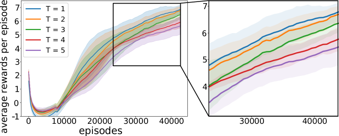
Figure 2: The effect of terminating options early, i.e., after T steps

This poses a dilemma that is specific to multi-agent systems: excessive terminations makes an agent’s behaviour unpredictable, while insufficient termination of options results in agents’ inflexibility towards changes[8]. We will refer to an agent’s flexibility as the ability to switch options in response to changes in others or the environment. Furthermore, we will use predictability to measure how far an agent will commit to its broadcast option. In this paper, we propose an approach called dynamic termination, which allows an agent to choose whether to terminate its current option according to the state and others’ options. This approach balances flexibility and predictability, combining the advantages of both.

An obvious approach to modelling dynamic termination is to use an additional controller, which decides whether to terminate or to continue with the current option at each step. In this paper, we incorporate termination as an additional option for the high-level controller. In this way, the Q-value of the newly introduced option is associated consistently with the Q-values of the original options, and our approach introduces negligible additional complexity to the original model. We evaluate our model on the standard multi-agent pursuit and taxi coordination tasks across a range of parameters. The results demonstrate that our dynamic termination model can significantly improve hierarchical multi-agent coordination and that it outperforms relevant state-of-the-art algorithms. The contributions of our work are as follows:

1. Based on the decentralized multi-agent options framework, we propose a novel dynamic termination scheme which allows an agent to flexibly terminate its current option. We show empirically that our model can greatly improve multi-agent coordination

2. We propose a delayed communication method for an agent to approximate the joint Q-value. This method allows us to use intra-option learning, and reduces potentially costly communication

3. We incorporate dynamic termination as an option to the high level controller network. This design introduces little additional model complexity, and allows us to represent the termination of all options in a consistent manner

In addition, we adopted several methods that benefits the model architecture and training: deep Q networks and parameter sharing reduce state space and model complexity; adapting intra-option learning [18] to multiple agents yields better sample efficiency; and an off-policy training scheme [7] for exploration.

2 Related Work

Makar et al.[11] appear to have been the first to combine multi-agent and hierarchical RL, through the MaxQ framework [2]. We build on their work, with the following changes: First, the use of tabular Q-learning is insufficient for large state spaces. Therefore, we adopt deep Q networks for parameterizing state and action spaces. Second, we adapt intra-option learning to multi-agent systems [18], which greatly improves the sample efficiency. Third, we adopt a delayed communication channel to prevent costly communication, and joint optimization. And finally, as options cannot be terminated before their predefined termination condition, tasks are limited to the use of perfect options and agents experience the delayed response problem.

Our solution to the delayed response problem is related to works on interrupting imperfect options, i.e., when the set of available options are not perfectly suited to the task, an agent can choose to terminate its options dynamically in order to improve its performance. Sutton et al.[18] introduced a mechanism for interrupting options whenever a better option appears, and Harutyunyan et al.[7] proposed a termination framework which improves upon this idea with better exploration. This is achieved by off-policy learning, which uses an additional behaviour policy for longer options.

Bacon et al.[1] proposed a dynamically terminating model for their Option-critic framework. In comparison, we use the Q-learning framework instead of policy gradient; and we focus on addressing the coordination problems in a multi-agent system. Moreover, our Q-value for dynamic termination does not depend on the currently executing option, which significantly reduces the model complexity and also improve sample efficiency due to off-policy training, i.e., the value of terminating can be learned with any executed option.

In the multi-agent learning literature, Riedmiller et al.[15] proposed the multi-option framework. This is a centralized model in which multiple agents are considered as a single meta-agent that chooses a joint option $\mathbf{o}=(o_{1},\ldots,o_{n})$. In contrast, our model uses a decentralized scheme where each agent $i$ chooses and executes its own option $o_{i}$. This reduces the action space of the high level controller from $|O|^{n}$ to $|O|$, where $O$ is the set of all options, and $n$ is the number of agents.

Our model also draws upon the independent Q-learning framework proposed by Tan[20], where each agent independently learns its own policy on primitive actions, while treating other agents as part of the environment. Additionally in our model, each agent conditions on the others’ broadcast options as part of its observation when choosing the next option. We will discuss the detailed formulation in section 4.

3 Basic Definitions

We first introduce the essential concepts in reinforcement learning (RL), followed by multi-agent RL, hierarchical RL, intra-option learning and off-policy termination.

A Markov Decision Process [17] is given by a tuple $\langle\mathcal{S},\mathcal{A},R,P,\gamma\rangle$, where $\mathcal{S}$ denotes a set of states, $\mathcal{A}$ a set of actions, $P$ the stationary transition probability $P(s_{t+1}|s_{t},a_{t})$ from state $s_{t}$ to state $s_{t+1}$ after executing action $a_{t}$, $R$ is the average reward function $r_{t}:=R(s_{t},a_{t})$, and $\gamma\in[0,1)$ is the discount factor. A policy $\pi(a_{t}|s_{t})$ is a distribution over actions $a_{t}$ given the state $s_{t}$. The objective of a RL agent is to learn an optimal policy $\pi^{*}$, which maximizes the expected cumulative discounted future rewards. The Q-value of the optimal policy conditions this return on an action $a_{t}$ that has been selected in a state $s_{t}$:

$$\footnotesize Q^{*}(s_{t},a_{t})=\operatorname{\mathbb{E}}\!\Big{[}{\textstyle\sum\limits_{\tau=0}^{\infty}}\,\gamma^{\tau}r_{t+\tau}\Big{]}=r_{t}+\gamma\max_{a^{\prime}}\operatorname{\mathbb{E}}\!\big{[}Q^{*}(s_{t+1},a^{\prime})\big{]}.$$ (1)

Q-learning learns the Q-value of the optimal policy by interacting with a discrete environment [22]. Continuous and high-dimensional states require function approximation [17], for example deep convolutional neural networks (DQN) [12, 13]. To improve the stability of gradient decent, DQN introduces an experience replay buffer to store transitions that have already been seen. Each update step samples a batch of past transitions and minimizes the mean-squared error between the left and right side of Equation 1.

In multi-agent reinforcement learning, $n$ agents interact with the same environment. The major difference to the single agent case is that the joint action space $\mathcal{A}=\mathcal{A}^{1}\times\cdots\times\mathcal{A}^{n}$ of all agents grows exponential in $n$. Independent Q-learning addresses this by decentralizing decisions [20]: each agent learns a Q-value function that is independent of the actions of all other agents. This treats others as part of the environment and can lead to unstable DQN learning [5]. Other approaches combine decentralized functions with a learned centralized network [14] or train decentralized Actor-Critic architectures with centralized baselines [4].

We now describe some important concepts related to hierarchical reinforcement learning (HRL). The Options Framework [18] is one of the most common HRL frameworks, which defines a two-level hierarchy, and introduces options as temporally extended actions. Options $o$ are defined as triples $\langle\mathcal{I}^{o},\beta^{o},\pi^{o}\rangle$, where $\mathcal{I}^{o}\subseteq\mathcal{S}$ is the initiation set and $\beta^{o}:\mathcal{S}\rightarrow[0,1]$ is the option termination condition. $\pi^{o}:\mathcal{S}\rightarrow\mathcal{A}$ is a deterministic option policy that selects primitive actions to achieve the target of the option. On reaching the termination condition in state $s^{\prime}$, an agent can select a new option from the set $\mathcal{O}(s^{\prime}):=\{o\,|\,s^{\prime}\in\mathcal{I}^{o}\}$. A Semi-Markov Decision Process (SMDP) [18] defines the optimal Q-value:

$$Q(s_{t},o_{t})\;\;=\;\;\operatorname{\mathbb{E}}\!\Big{[}{\textstyle\sum\limits_{\tau=0}^{k-1}}\gamma^{\tau}r_{t+\tau}+\,\gamma^{k}\kern-8.61108pt\max_{o^{\prime}\in\mathcal{O}(s_{t+k})}\kern-8.61108ptQ(s_{t+k},o^{\prime})\Big{]}\,,$$ (2)

where $k$ refers to the number of steps until the termination condition $\beta^{o_{t}}(s_{t+k})=1$ is fulfilled.

To improve sample efficiency, Intra-option Learning [18, 19] was proposed as an off-policy learning method which at each time step $t$ updates all options that are in agreement with the executed action, i.e. $\forall o\in\{o\,|\,\pi^{o}(s_{t})=a_{t}\}$ holds:

$$Q(s_{t},o) = r_{t}+\gamma\operatorname{\mathbb{E}}\!\big{[}U(s_{t+1},o)\big{]}$$ (3)

$$U(s,o) = \big{(}1-\beta^{o}(s)\big{)}\,Q(s,o)\;+\,\beta^{o}(s)\kern-2.15277pt\max_{o^{\prime}\in\mathcal{O}(s)}\kern-4.30554ptQ(s,o^{\prime}).$$

Here $U(s_{t+1},o)$ is the TD-target  [21]: if $o$ is terminating in the next state, the TD-target will be the value of choosing the next optimal option. If not, the target will be the value of continuing with option $o$. Updating multiple options vastly improves the efficiency of training. Consider a grid-world navigation case where an agent is going for some goal location, and each coordinate corresponds to the sub-goal of an option. When the agent takes a primitive action $a_{t}^{j}$ and reaches the next position, all options $o^{j}$ that would have chosen that action will be updated. Each transition updates therefore a significant fraction of the options, which massively improves sample efficiency.

As introduced by Sutton et al. [18], when the set of available options are not suited to the task, an agent can improve its performance by terminating at each step and switching to an optimal option. Harutyunyan et al. [7] have shown that this approach improves the agent’s performance significantly, but has an adverse effect on exploration: temporally extended options can explore the state space more consistently, which is lost by early termination. The authors therefore advocate the use of intra-option learning to update the Q-value off-policy, while executing a different exploration policy that follows a selected option for multiple steps before terminating.

4 Method

In this section we will present our framework for deep decentralized hierarchical multi-agent Q-learning. Our model uses delayed communication to approximate the decisions of a centralized joint policy, which avoids many problems usually associated with joint optimization. This induces new challenges such as a delayed response of agents, and requires us to define a novel dynamic termination update equation.

Figure 3: Dynamic termination Q-value network architecture.

Delayed Communication: A straightforward application of decentralized multi-agent approaches like independent Q-learning (IQL) [20] to the Options framework [18] would yield agents that make decisions independent of each other. Agent $j$ would estimate the Q-value (see Equation 2)

$$Q^{j}_{\text{iql}}(s_{t},o^{j}_{t}):=\operatorname{\mathbb{E}}\!\Big{[}{\textstyle\sum\limits_{\tau=0}^{k-1}}\gamma^{\tau}r_{t+\tau}\!+\!\gamma^{k}\!\!\max_{{o^{\prime}}^{j}\in\mathcal{O}^{j}}\!\!Q^{j}_{\text{iql}}(s_{t+k},o^{\prime j})\Big{]},$$ (4)

and select the option $o^{j}_{t}$ that maximizes it. Here other agents are treated as stationary parts of the environment, which can lead to unstable training when those agents change their policy. The best way to avoid this instability would be learn the Q-value w.r.t. the joint option of all agents $\mathbf{o}_{t}:=(o^{1}_{t},\ldots,o^{n}_{t})$, i.e. $Q_{\text{joint}}(s_{t},\mathbf{o}_{t})$  [15]. While these joint Q-values allow training in a stationary environment, decisions require to maximize over Q-values of all possible joint options. As the number of joint options grows exponentially in the number of agents $n$, and joint optimization would require a vast communication overhead, this approach is not feasible in decentralized scenarios.

Instead we propose to use a delayed communication channel over which agents signal the new option they switched to after each termination. This reduces potentially costly communication and allows each agent $j$ access to all other agents’ options of the previous time step $\mathbf{o}^{-j}_{t-1}:=(o^{1}_{t-1},\ldots,o^{j-1}_{t-1},o^{j+1}_{t-1},\ldots,o^{n}_{t-1})$. Agents can approximate the joint Q-value by conditioning on this information, that is, by choosing options $o^{j}_{t}$ that maximize the delayed Q-value $Q^{j}(s_{t},\mathbf{o}^{-j}_{t-1},o^{j}_{t})$. Note that the approximation is exact if no other agent terminates at time $t$. The optimality of the agents’ decisions depends therefore on the frequency with which agents terminate their options.

Multi-agent Intra-Option Learning: As introduced in the previous section, the intra-option learning method (Equation 3) efficiently associates options with primitive actions. In our decentralized multi-agent options model, agent $j$ selects an option according to $Q^{j}(s_{t},\mathbf{o}^{-j}_{t-1},o^{j})$, which is defined as

$$Q^{j}(s_{t},\mathbf{o}^{-j}_{t-1},o^{j}) := \operatorname{\mathbb{E}}\big{[}r_{t}+\gamma U^{j}(s_{t+1},\mathbf{o}^{-j}_{t},o^{j})\big{]}$$ (5)

$$U^{j}(s_{t+1},\mathbf{o}^{-j}_{t},o^{j}) := \big{(}1-\beta^{o^{j}}\!(s_{t+1})\big{)}\;Q^{j}(s_{t+1},\mathbf{o}^{-j}_{t},o^{j})$$

$$+\,\beta^{o^{j}}\!(s_{t+1})\!\max_{o^{\prime j}\in\mathcal{O}^{j}}\!\!Q^{j}(s_{t+1},\mathbf{o}^{-j}_{t},o^{\prime j}).$$

We can learn $Q^{j}$ by, for example, minimizing the mean-squared TD error  [17] between the left and right side of Equation 5. In line with intra-option learning, we update the Q-values of all options $o^{j}$ that would have executed the same action $a^{j}_{t}$ as the actually executed option $o^{j}_{t}$. Note that due to our delayed communication channel, the executed options of all other agents are known after the transition to $s_{t+1}$ and can thus be used to compute the target $U^{j}(s_{t+1},\mathbf{o}^{-j}_{t},o^{j})$, that is, the Q-value of either following the option $o^{j}$ if $\beta^{o^{j}}\!(s_{t+1})=0$, or terminating and choosing another option greedily if $\beta^{o^{j}}\!(s_{t+1})=1$.

Dynamic Option Termination: As mentioned above, the delayed Q-value defined in Equation 5 only approximates the joint Q-value function. This approximation will deteriorate when other agents terminate, but sometimes agents can also benefit from early termination, as shown in Figure 1(b). Additionally, options are usually pre-trained and have to cover a large range of tasks, without being able to solve any one task perfectly. Being able to prematurely terminate options can increase the expressiveness of the learned policy dramatically.

The easiest way to use partial options is to modify the termination conditions $\beta^{o^{j}}(s)$. In particular, we denote choosing the option with the largest Q-value (Eq. 5) at each time step as greedy termination. Following [7] we combined this approach with an exploration policy that terminates executed options with a fixed probability $\rho=0.5$ to allow for temporally extended exploration. During testing the agent is nonetheless allowed to terminate greedily at every step if the Q-value of another option is larger.

Although greedy termination has been shown to improve the performance of individual agents with imperfect options [7], the agent’s behaviour will become less predictable for others. In particular, agents that utilize the delayed Q-value of Equation 5 will make sub-optimal decisions whenever another agent terminates. To increase the predictability of agents, while allowing them to terminate flexibly when the task demands it, we propose to put a price $\delta$ on the decision to terminate the current option. Option termination is therefore no longer hard-coded, but becomes part of the agent’s policy, which we call dynamic termination. This can be represented by an additional option $o^{j}=T$ for agent $j$ to terminate. Note that, unlike in the Options framework, we no longer need a termination function $\beta^{o^{j}}\!(s_{t})$ for each option $o^{j}$. It is sufficient to compare the value of the previous option $Q^{j}(s_{t},\mathbf{o}^{-j}_{t-1},o^{j}_{t-1})$ with the value of termination $Q^{j}(s_{t},\mathbf{o}^{-j}_{t-1},T)$. Evaluating $o^{j}=T$ is computationally similar to evaluating the termination condition $\beta^{o}$. Dynamic termination therefore has a similar cost to traditional termination.

The optimal behaviour for a given punishment $\delta$ is the fix-point of the novel dynamic termination Bellman equation:

$$Q^{j}(s_{t},\mathbf{o}_{t-1}^{-j},o^{j}\!\neq\!T) \kern-6.45831pt:=\kern-6.45831pt \operatorname{\mathbb{E}}\big{[}r_{t}\!+\gamma\max\limits_{\kern-3.01389pto^{\prime j}\in\{o^{j},T\}}{Q^{j}(s_{t+1},\mathbf{o}_{t}^{-j}\kern-4.30554pt,o^{\prime j})\big{]}},$$

$$Q^{j}(s_{t},\mathbf{o}_{t-1}^{-j},o^{j}\!=\!T) := \max\limits_{o^{\prime j}\in\mathcal{O}^{j}}{Q^{j}(s_{t},\mathbf{o}_{t-1}^{-j},o^{\prime j})}\,-\,\delta\,.$$ (6)

Similarly to Equation 5, Equation 6 allows intra-option learning and can be applied to all options $o^{j}$ that would have selected the same action as the executed option $o^{j}_{t}$. Note that the termination option $T$ can always be updated, as it does not depend on the transition.

Deep Q-learning: A group of $n$ agents can be trained using a deep Q-network $Q_{\theta}$ [12], parameterized by $\theta$. The architecture is shown in Figure 3: each agent $j$ selects and executes the next option based on the current state (i.e. grid-word image) $s_{t}$ and the last known options $\mathbf{o}^{-j}_{t-1}$ of all the other agents. A centralized manager is not needed, and the options must only be broadcast after an agent chose to select a new option. The Q-value of choosing an option is updated by temporal difference learning with experience replay, which is the established standard procedure in deep Q-learning [12]. To reduce the number of parameters, we let all the agents share $\theta$, and the model is thus updated using the experiences collected by all the agents. To differentiate the behaviour of different agents, the presented grid-world image contains a dedicated channel that encodes the current agent’s state. These design decisions follow previous work in deep multi-agent learning [4, 14] and drastically reduce training time with very little impact on the performance in large domains.

At each transition $t$, the Q-values of all options $o^{j}$, that would execute the same action as the executed option $o_{t}^{j}$, and the termination option $T$ are updated by gradient descent on the sum of their respective losses

$$\mathcal{L}^{o}_{j,t}\big{[}\theta\big{]} := \Big{(}r_{t}\!+\!\gamma\max_{o^{\prime}\in\{o,T\}}Q_{\theta}(s_{t+1},\mathbf{o}^{\!-j}_{t}\!\!,o^{\prime})-Q_{\theta}(s_{t},\mathbf{o}^{-j}_{t-1},o)\Big{)}^{\!2},$$

$$\mathcal{L}^{T}_{j,t}\big{[}\theta\big{]} := \Big{(}\max\limits_{o^{\prime}\in\mathcal{O}^{j}}Q_{\theta}(s_{t},\mathbf{o}_{t-1}^{-j},o^{\prime})-\delta-Q_{\theta}(s_{t},\mathbf{o}_{t-1}^{-j},T)\Big{)}^{\!2}\kern-2.15277pt.$$

The total loss for a batch of $m$ transitions with $n$ agents is

$$\mathcal{L}\big{[}\theta\big{]}\quad:=\quad\frac{1}{mn}\sum_{t=0}^{m-1}\sum_{j=1}^{n}\Big{(}\mathcal{L}^{T}_{j,t}\big{[}\theta\big{]}\;+\kern-8.61108pt\sum_{\pi^{o}(s_{t})=a^{j}_{t}}\kern-8.61108pt\mathcal{L}^{o}_{j,t}\big{[}\theta\big{]}\Big{)}\,.$$ (7)

5 Experiments

Table 1: Example $16\times 16$ Grid-world

	predictability			flexibility
	option changes			option changes	steps to change
	all	near	far	all	all
dynamic	24.1%	28.1%	16.8%	63%	1.61
greedy	59.9%	57.9%	52.8%	77%	1.15
option	10.9%	10.9%	9.5%	3%	6.86

Table 2: Flexibility and Predictability Results. Near/far refers to whether an agent is within distance $=4$ to a passenger. Steps to change denotes the number of steps from the new passenger is placed to the agent’s option change.

We will first evaluate the flexibility and predictability of our dynamically terminating agent, followed by the impact of dynamic termination on the agents’ performance.

Experimental Setup: Figure 2 shows a $16\times 16$ grid-world of the taxi pickup as observed by the green agent, which includes the passengers, the other agents and their broadcast options. The landmarks of distance $L=3$ show the destinations of options that are currently visible to the agent. This raises our first challenge: in order to reach a passenger that stands outside the landmarks, an agent needs to correctly switch between options.

In the Taxi Pickup Task $m$ passengers are randomly distributed in each episode. An agent is rewarded $r=1$ when occupying the same grid as a passenger, and each step incurs a cost of $-0.01$. Apart from landmark switching, the agents need to interpret others’ behaviours to avoid choosing the same passenger, as well as responding quickly to changes such as when a passenger is picked up by another agent.

In the Pursuit Task agents try to catch randomly distributed prey by cooperating with others. We refer to the task as $k$-agent pursuit, where a successful capture requires at least $k$ agents occupying $k$ positions adjacent to the prey, which rewards each participating agent $r=1$. This task relies heavily on agents coordination. In particular, when close to a specific prey, agents need to observe others and switch between options to surround the prey; whereas when faraway, agents need to agree on and commit to go for the same prey.

Algorithms and Training: Having described the settings, we now introduce the detailed training procedures of the SMDP and option policies, before comparing the four types of agents.

The Policy of Options adopts a local perspective, and navigates the agent to the option’s destination. Specifically, we use a DQN of $2$ convolutional layers (kernel size 2) with max-pooling, followed by $4$ fully-connected layers (size 300). The input is the destination coordinate with the grid-world image, and the output is a primitive action in {N, S, E, W, Stay}.

The SMDP Policies are trained through intra-option learning for all agent types. The inputs are $4$-channel grid-world images as in Figure 3, which represents the agent, the preys (or passengers), the other agents, and lastly, the options broadcast by other agents (except for IQL). The DQN contains 2 convolutional layers (kernel size 3), max pooling, and 4 fully-connected layers (size 512). We use experience replay with a replay buffer of size 100,000.

Self-Play is used in the experiments, and our decentralized agents share the same DQN parameters (not states) [14]. This allows us to scale up the number of agents without additional parameters; and the trained model can directly transfer to more agents during testing. Moreover, self-play creates an important link between the predictability of an individual agent and of the society.

The four types of agents are as follows:

1. Option Termination Agent executes its option until the natural termination condition is met.

2. Greedy Termination Agent terminates every step and switches to the optimal option. For better exploration during training, an additional behaviour policy is used for experience collection. For fairness of comparison, this exploration policy which terminates with probability $\rho=0.5$ (tuned for the greedy agent) is applied across all agent types.

3. Dynamic Termination Agent is our proposed algorithm that chooses whether to terminate the current option at each step. $\delta$ is the termination penalty.

4. IQL is independent Q-learning, where agents option broadcasts are disabled. IQL (greedy) and IQL ($\delta$) refers to IQL agents using greedy or dynamic termination.

(a) $19\times 19$ taxi with 10 agents

(b) $19\times 19$ pursuit with 10 agents

Figure 4: Results from Taxi Pickup and Pursuit Tasks

Note: Every point per 500 episode is the testing result averaged over 100 random episodes and 5 seeds. The shaded area shows standard deviation across seeds.

		taxi			2 agent pursuit			3 agent pursuit
		n=5, m=10		n=10, m=20	n=3, m=5		n=10, m=10	n=3, m=5
Agents		19x19	25x25	19x19	16x16 (r=1)	19x19 (r=1)	19x19 (r=1)	10x10 (r=1)	16x16 (r=2)
Dynamic	$\delta$ = 0.1	7.89	5.75	15.29	10.24	9.30	12.50	6.71	10.38
	$\delta$ = 0	6.58	3.28	11.81	6.73	4.07	5.38	5.53	6.54
Greedy		6.62	3.23	12.39	7.36	3.74	4.65	5.89	6.40
Option		-0.32	-0.94	0.52	5.47	-1.82	-1.42	-3.77	5.20
IQL	$\delta$ = 0.1	7.11	5.09	12.02	-1.57	-2.29	-0.84	-1.62	-0.59
	greedy	6.08	2.79	9.06	-2.12	-2.49	-1.64	-2.13	-0.42

Table 3: Average reward after training for Taxi and Pursuit tasks. n is the number of agents and m is the number of passengers (preys). NxN denotes grid-world size, k agent pursuit denotes the required number of agents for capture, and r is the capture range.

Results: The delayed response problem reveals that agents need to be flexible enough to change their options when the situation changes, but also predictable enough not to interfere in other agents’ plans too frequently. Table 2 shows experimental measurements to showcase these conflicting goals for the investigated termination methods. We measure the agents’ flexibility in the single-agent taxi domain. 100 episodes are initialized with 5 random passengers. During each episode, one additional passenger is placed near the agent at step $T$ and we observe how quickly the agent adjusts to the new situation. We report the percentage of option changes at step $T+1$ and the average number of steps till the agent changes options. Note that dynamic termination allows to react almost as flexible to the changed situation as the greedy termination.

For predictability, we measure the average probability to change the option in the multi-agent taxi task for two cases: when the agent is near (within distance 4) or far from its closest passenger. This is an imperfect measurement, as we cannot distinguish the effect of termination on other agents. While options need to change close to a passenger due to imperfect options, the behavior of dynamic termination is much closer to standard option termination when far away. Note that this effect is marginal for the other techniques, which indicates that our method may purposefully refrain from changing to better options to avoid interrupting other agent’s plans.

Performance: Figure 4(a) shows the results from the taxi pickup task. The option termination agent fails due to its inflexibility to switch options. In contrast, our dynamic ($\delta=0.15$) agent is highly flexible. Moreover compared with greedy and IQL, its high predictability indeed helps the agents to interpret others’ intentions and better distribute their target passengers. Figure 4(b) shows the results on the pursuit task, where at least two agents need to surround a prey within capture range $=1$. Seen from the IQL agents’ low performance, option broadcasting and interpreting others’ behaviours are crucial to this task. Our dynamic termination agent ($\delta=0.1$) significantly outperforms all other agents. Compared with the greedy agents, we can conclude that predictability significantly helps our dynamic agents to stay committed and succeed in cooperation.

Finally, we present the performance of all agents across different tasks and varying parameters in Table 3. Firstly, the option termination agent has difficulty with tasks which require higher level of accuracy and quick responses, such as the taxi tasks and pursuit with capture range $=1$. However, it works well with tasks which require coordination but less flexibility, such as the $16\times 16$ 3 agent pursuit with capture range 2, which shows the advantage of predictability on cooperation. The performance of greedy termination agents decreases significantly in larger grid-world sizes, and when commitment is essential, such as the $16\times 16$ 3 agent pursuit with capture range 2. Our dynamically terminating agent performs well across all tasks, as it balances well between flexibility and predictability. The IQL agents performs well in the taxi task. However, they fail to learn the pursuit tasks where foreseeing others’ behaviours is essential to coordination.

6 Conclusions and Future Work

In this paper, we identified the delayed response problem, that occurs when hierarchical RL is combined with multi-agent learning. To address this challenge, we investigated existing approaches of greedy option termination in single agent learning. However, this method introduces a new dilemma specific to multi-agent systems: as an agent broadcasts its current options to indicate its subsequent behaviours, frequent changes in options will result in its behaviour being less predictable by others. Therefore, to balance flexibility with predictability, we introduced dynamic termination, which enables agents to terminate their options flexibly according to the current state. We compared our model with current state of the art algorithms on multi-agent pursuit and taxi tasks with varying task parameters, and demonstrated that our approach outperformed the baselines through flexibly adapting to the task requirements. For future work, we are interested in applying the dynamic termination framework to traffic simulations, such as junction and highway management.

References

- [1] Bacon, P.L., Harb, J., Precup, D.: The option-critic architecture. In: AAAI. pp. 1726–1734 (2017)
- [2] Dietterich, T.G.: Hierarchical reinforcement learning with the maxq value function decomposition. Journal of Artificial Intelligence Research 13, 227–303 (2000)
- [3] Foerster, J., Assael, I.A., de Freitas, N., Whiteson, S.: Learning to communicate with deep multi-agent reinforcement learning. In: Advances in Neural Information Processing Systems. pp. 2137–2145 (2016)
- [4] Foerster, J., Farquhar, G., Afouras, T., Nardelli, N., Whiteson, S.: Counterfactual multi-agent policy gradients. arXiv preprint arXiv:1705.08926 (2017)
- [5] Foerster, J., Nardelli, N., Farquhar, G., Afouras, T., Torr, P.H.S., Kohli, P., Whiteson, S.: Stabilising experience replay for deep multi-agent reinforcement learning. In: Proceedings of the 34th International Conference on Machine Learning. Proceedings of Machine Learning Research, vol. 70, pp. 1146–1155 (2017), http://proceedings.mlr.press/v70/foerster17b.html
- [6] Giannakis, M., Louis, M.: A multi-agent based system with big data processing for enhanced supply chain agility. Journal of Enterprise Information Management 29(5), 706–727 (2016)
- [7] Harutyunyan, A., Vrancx, P., Bacon, P.L., Precup, D., Nowe, A.: Learning with options that terminate off-policy. arXiv preprint arXiv:1711.03817 (2017)
- [8] Jennings, N.R.: Commitments and conventions: The foundation of coordination in multi-agent systems. The knowledge engineering review 8(3), 223–250 (1993)
- [9] Lesser, V., Ortiz Jr, C.L., Tambe, M.: Distributed sensor networks: A multiagent perspective, vol. 9. Springer Science & Business Media (2012)
- [10] Lin, K., Zhao, R., Xu, Z., Zhou, J.: Efficient large-scale fleet management via multi-agent deep reinforcement learning. arXiv preprint arXiv:1802.06444 (2018)
- [11] Makar, R., Mahadevan, S., Ghavamzadeh, M.: Hierarchical multi-agent reinforcement learning. In: Proceedings of the fifth international conference on Autonomous agents. pp. 246–253. ACM (2001)
- [12] Mnih, V., Kavukcuoglu, K., Silver, D., Graves, A., Antonoglou, I., Wierstra, D., Riedmiller, M.: Playing Atari with deep reinforcement learning. In: NIPS Deep Learning Workshop (2013)
- [13] Mnih, V., Kavukcuoglu, K., Silver, D., Rusu, A.A., Veness, J., Bellemare, M.G., Graves, A., Riedmiller, M., Fidjeland, A.K., Ostrovski, G., et al.: Human-level control through deep reinforcement learning. Nature 518(7540), 529 (2015)
- [14] Rashid, T., Samvelyan, M., de Witt, C.S., Farquhar, G., Foerster, J., Whiteson, S.: Qmix: Monotonic value function factorisation for deep multi-agent reinforcement learning. arXiv preprint arXiv:1803.11485 (2018)
- [15] Riedmiller, M., Withopf, D.: Effective methods for reinforcement learning in large multi-agent domains (leistungsfähige verfahren für das reinforcement lernen in komplexen multi-agenten-umgebungen). it-Information Technology 47(5), 241–249 (2005)
- [16] Stone, P., Veloso, M.: Multiagent systems: A survey from a machine learning perspective. Autonomous Robots 8(3), 345–383 (2000)
- [17] Sutton, R.S., Barto, A.G.: Reinforcement Learning: An Introduction. MIT Press (1998)
- [18] Sutton, R.S., Precup, D., Singh, S.: Between mdps and semi-mdps: A framework for temporal abstraction in reinforcement learning. Artificial intelligence 112(1-2), 181–211 (1999)
- [19] Sutton, R.S., Precup, D., Singh, S.P.: Intra-option learning about temporally abstract actions. In: ICML. vol. 98, pp. 556–564 (1998)
- [20] Tan, M.: Readings in agents. chap. Multi-agent Reinforcement Learning: Independent vs. Cooperative Agents, pp. 487–494 (1998)
- [21] Tesauro, G.: Temporal difference learning and td-gammon. Communications of the ACM 38(3), 58–68 (1995)
- [22] Watkins, C., Dayan, P.: Q-learning. Machine Learning 8, 279–292 (1992)