Gravitational wave signatures of ultralight vector bosons
from black hole superradiance

Abstract

In the presence of an ultralight bosonic field, spinning black holes are unstable to superradiance. The rotational energy of the black hole is converted into a non-axisymmetric, oscillating boson cloud which dissipates through the emission of nearly monochromatic gravitational radiation. Thus, gravitational wave observations by ground- or space-based detectors can be used to probe the existence of dark particles weakly coupled to the Standard Model. In this work, we focus on massive vector bosons, which grow much faster through superradiance, and produce significantly stronger gravitational waves compared to the scalar case. We use techniques from black hole perturbation theory to compute the relativistically-correct gravitational wave signal across the parameter space of different boson masses and black hole masses and spins. This fills in a gap in the literature between flatspace approximations, which underestimate the gravitational wave amplitude in the non-relativistic limit, and overestimate it in the relativistic regime, and time-domain calculations, which have only covered a limited part of the parameter space. We also identify parameter ranges where overtone superradiantly unstable modes will grow faster than the lower frequency fundamental modes. Such cases will produce a distinct gravitational wave signal due to the beating of the simultaneously populated modes, which we compute.

I Introduction

A common feature in extensions to the Standard Model of particle physics, and low-energy effective theories of quantum gravity, is the prediction of light bosonic particles. Examples include massive bosons in open string scenarios Arvanitaki et al. (2010); Jaeckel and Ringwald (2010); Arvanitaki and Dubovsky (2011), dark photons as a dark matter candidate Agrawal et al. (2018); Essig et al. (2013), non-minimally coupled bosons as dark energy on cosmological scales De Felice et al. (2016a, b), and the axion as a solution to the CP problem in QCD Peccei and Quinn (1977); Weinberg (1978). Direct detection methods have so far been unsuccessful in revealing the existence of such particles. However, the superradiant instability of black holes (BHs) provides a way to probe ultralight bosons without assuming any specific coupling to other fields, except for the minimal one to gravity. Especially in light of the increasing reach of observatories like LIGO/Virgo Abbott et al. (2016, 2019), there has been strong interest in using gravitational wave (GW) observations to search for evidence of these particles.

A bosonic field incident on a spinning BH with real frequency $\omega_{R}$ and azimuthal mode number $m$ will induce a flux of energy $\mathscr{E}$ and angular momentum $\mathscr{L}$ across the BH horizon with ratio $\mathscr{L}/\mathscr{E}=m/\omega_{R}$. Combining the first and second laws of BH thermodynamics implies that $\mathscr{E}-\Omega_{H}\mathscr{L}>0$ Bardeen et al. (1973), where $\Omega_{H}$ is the horizon frequency of the BH. As a consequence, if the superradiance condition $0<\omega_{R}<m\Omega_{H}$ is satisfied, the energy and the angular momentum flux through the horizon become negative, and the field will be superradiantly scattered, gaining energy at the expense of the BH’s rotational energy Press and Teukolsky (1972). Bosonic fields with non-vanishing rest mass $m_{\gamma}$ (and hence mass parameter $\mu:=m_{\gamma}/\hbar$) can form states that are gravitationally bound to the BH and have a continuous flux across the horizon. Bound states that satisfy the superradiant condition grow exponentially in time, and can be characterized by a complex frequency $\omega=:\omega_{R}+i\omega_{I}$ (where we take the convention that $\omega_{I}>0$ for a growing mode).

Though the above discussion assumes an adiabatic description, this has been found to be a good approximation, even in the fully non-linear scenario East (2018); East and Pretorius (2017); the BH loses mass and angular momentum until it spins down to the point where $\omega_{R}\approx m\Omega_{H}$ and the superradiance condition is saturated. During the growth of the cloud, the field can extract an excess of $\sim 9\%$ of the BH mass before the instability is saturated East and Pretorius (2017) and the BH-cloud configuration reaches a quasi-equilibrium configuration.

The existence of such scalar or vector bosonic clouds with an exponentially large occupation number around spinning BHs has several potentially observable consequences. The reduction in the rotational energy of the BH yields gaps in the spin-mass plane, which could be investigated with direct spin and mass measurements of a large BH population Arvanitaki and Dubovsky (2011); Davoudiasl and Denton (2019); Cardoso et al. (2018). Additionally, clouds of bosons can change the dynamical behavior, and emitted gravitational radiation, of binary BHs, giving rise to transition resonances between cloud field modes during the inspiral, or other tidal effects Baumann et al. (2019a); Berti et al. (2019); Zhang and Yang (2019a, b). Finally, the boson cloud will oscillate and produce gravitational radiation, even in its saturated state. Hence, the cloud slowly dissipates through emitting GWs. These sources might be resolved individually Arvanitaki et al. (2015, 2017), or contribute to a GW stochastic background Tsukada et al. (2019); Brito et al. (2017a, b). The nearly monochromatic gravitational radiation roughly falls into the LIGO band for boson masses $m_{\gamma}\in(10^{-11},10^{-14})$ eV and the LISA band for boson masses $m_{\gamma}\in(10^{-16},10^{-20})$ eV, and could be detected directly given detailed predictions across the possible parameter space.

Most studies so far have concentrated on the scalar case – i.e., a spin-0 boson – in part due to technical difficulties associated with tackling the vector case, which we discuss below. However, vector bosons can actually be better constrained by observations as their superradiant growth rates and the resulting gravitational wave luminosities are orders of magnitude higher than scalars. In this work, we provide detailed predictions for the gravitational signals originating from a vector boson cloud around a spinning BH arising from superradiance that can be used in performing searches/placing bounds using upcoming GW observations.

Bound modes for a massive vector (or Proca) field on a Kerr spacetime are characterized by a time-dependence with harmonic form, i.e., $e^{-i\omega t}$ with $\omega_{R}<\mu$, and $\omega_{I}$ quantifying the change in amplitude over time due to the dissipative boundary conditions at the horizon. Hence, a quasi-normal field mode with azimuthal number $m$ is superradiant when $0<\omega_{R}<m\Omega_{H}$ and $0<\omega_{I}$ are satisfied. In the non-relativistic limit, $\mu M\ll 1$, the Proca field equations on a fixed Kerr spacetime with mass $M$ reduce to a set of Schrödinger-type equations, which are readily solved Baryakhtar et al. (2017). In this limit, the real frequency is given by

$$\frac{\omega_{R}}{\mu}\approx 1-\frac{\mu^{2}M^{2}}{2(|m|+\hat{n}+S+1)^{2}}+\mathcal{O}((\mu M)^{4})$$ (1)

and depends on the azimuthal mode $m$, overtone $\hat{n}$, and polarization state $S\in\{-1,0,1\}$ of the massive vector field. The imaginary part of the frequency can be found by performing a matching procedure at the BH horizon Baryakhtar et al. (2017); Baumann et al. (2019a, b). Solving the linear, but fully relativistic, mode equations, however, has been a challenge due to the fact that these equations do not decouple in the usual Teukolsky formalism. Alternative approaches include expanding in the limit of low BH spin Pani et al. (2012), utilizing time domain calculations Witek et al. (2013); East (2017), or numerically solving the coupled elliptic differential equations for the superradiant modes Cardoso et al. (2018). Recently, however, Frolov et al. Frolov et al. (2018) (henceforth FKKS), have extended the ansatz found in Ref.  Lunin (2017) in the massless case (see also Ref. Krtouš et al. (2018)), to massive vector fields. Based on the conformal Killing-Yano 2-form, this ansatz separates the Proca quasi-normal mode equations on the Kerr-NUT-(A)dS family of spacetimes. We use this approach here, in which finding the spectrum of Proca modes reduces to solving two decoupled, differential eigenvalue problems, to systematically cover the parameter space of superradiantly unstable modes. One of the new results presented here is that, for superradiantly unstable modes with $m>1$, overtone modes ($\hat{n}>0$) can have faster growth rates (but greater $\omega_{R}$ values) than the fundamental ($\hat{n}=0$) modes. This occurs for near-extremal spins in the relativistic regime for $m=2$, moderately high spins for $m=3$, and even for non-relativistic values for $m\geq 4$. In such cases, the overtone modes will reach saturation first, and then begin to decay as the fundamental mode grows, leading to a unique GW signal with multiple frequency components, including a lower frequency beating, or “transition” signal Baryakhtar et al. (2017), as we detail here.

In contrast to a compact object binary, the GWs from a bosonic cloud around a spinning BH cannot be approximated by a series of multipoles in a post-Newtonian framework. The characteristic length scale of the bosonic condensate $r_{c}$ can be comparable to, or much larger, than the wavelength of the emitted gravitational radiation (depending on the field’s mass): $\lambda_{\text{GW}}\gg r_{c}$. Hence, the quadrapole GW formula breaks down in much of the parameter space. In Ref. Baryakhtar et al. (2017), the GWs from vector boson clouds were calculated in the non-relativistic limit on a flat spacetime. However, as explained there, even in calculating the leading order non-relativistic result, the effect of the BH spacetime must be taken into account, and can increase the GW power by an estimated factor of $10$. References East (2017, 2018) computed the GW luminosity using fully relativistic time-domain simulations, but due to the computational expense, they only covered a limited number of cases in the relativistic regime. In this work, we compute GWs using the Teukolsky formalism Teukolsky (1973); Press and Teukolsky (1973), which captures linear metric perturbations on a Kerr background, across the entire frequency spectrum. The differential equations of this formalism are of the Sturm-Liouville type, and can be solved using a Green’s function approach. The gravitational radiation at future null infinity is determined by convolving this Green’s function with the source functions provided by the solutions to the Proca field equations. Gravitational wave modes and energy flux can then be projected out of the linear gravitational perturbations at future null infinity. This allows us to obtain accurate predictions for the GW amplitude and frequency across the parameter space of Proca masses and BH masses and spins, filling in the gap in the literature.

We also describe the evolution of vector boson clouds, assuming the superradiant instability is triggered by a small seed perturbation—e.g. a quantum fluctuation, and making use of a quasi-adiabatic description (which is a good approximation as indicated by East (2018); Ficarra et al. (2019)). Generically, the cloud will grow to saturation and then, on a longer timescale, dissipate through GW emission. We estimate how the frequency and amplitude of the emitted GWs change due to the secular loss of mass and angular momentum due to radiation.

This paper is structured in the following way. In Sec. II.1, we briefly introduce the Kerr geometry, and we review how the FKKS ansatz separates the Proca equations on Kerr in Sec. II.2. We describe how we solve the radial and angular equations to obtain the superradiant modes in Sec. II.3, and we detail how we normalize these modes in Sec. II.5. In Sec. II.4, we present the exponentially growing solutions to the Proca field equations. In Secs. III.1 and III.2, we review the Teukolsky formalism and associated Green’s function method we use to calculate the GWs. We present results for the gravitational radiation in Sec. IV, including the frequency and observability of GWs from ultralight vector boson clouds in Sec. IV.3. In Sec. V, we discuss our results and conclude. We use units with $G=c=1$ and the $(-,+,+,+)$ metric signature throughout the paper.

II The Proca field solution

II.1 Kerr spacetime

We ignore any non-linear interactions and solve the test-field Proca equations on a spinning BH background $g_{\mu\nu}\rightarrow g_{\mu\nu}^{\text{Kerr}}$ characterized by the BH mass $M$ and spin parameter $a=J/M$ (where $J$ is the BH’s angular momentum). Following Ref. Frolov et al. (2018), the Kerr geometry in canonical coordinates $(\tau,\zeta,y,\psi)$ takes the form

$$\begin{aligned} ds^{2}=\frac{\Xi}{\Pi}d\zeta^{2}&\ +\frac{\Pi}{\Xi}(d\tau+y^{2}d\psi)^{2}\\ &\ +\frac{\Xi dy^{2}}{y^{2}-a^{2}}-\frac{y^{2}}{\Pi}(d\tau^{2}+\zeta^{2}d\psi)^{2},\end{aligned}$$ (2)

with $\Xi:=y^{2}-\zeta^{2}$ and $\Pi:=-\zeta^{2}+2iM\zeta+a^{2}$. The canonical coordinates are related to the usual Boyer-Lindquist coordinates by $\tau=t-a\phi$, $\zeta=ir$, $y=a\cos\theta$, and $\psi=\phi/a$. As a member of the Kerr-NUT-(A)dS family of spacetimes, a spinning BH spacetime has a timelike $\boldsymbol{\xi}:=\partial_{\tau}$ and axial $\boldsymbol{\eta}:=\partial_{\psi}$ Killing field. In addition, this set of solutions admits more “hidden” symmetries, which were used in Ref. Frolov et al. (2018) to construct an ansatz to separate the massive vector field equation. Among others, one can construct a non-degenerate closed conformal Killing-Yano 2-form $\boldsymbol{h}$. The tensor components of this symplectic form are constructed from $\nabla_{\alpha}h_{\beta\gamma}=2g_{\alpha[\beta}\xi_{\gamma]}$, where $\xi_{\mu}$ are the components of the timelike Killing field $\boldsymbol{\xi}$. Therefore, $\boldsymbol{h}$ takes the form

$$\boldsymbol{h}=\zeta d\zeta\wedge(d\tau+y^{2}d\psi)+ydy\wedge(d\tau+\zeta^{2}d\psi)$$ (3)

in canonical coordinates, which we utilize in the next section to present the separated Proca equation.

II.2 Field equations

Disregarding any self-interactions of the massive vector, the field equations are

$$\nabla_{\mu}F^{\mu\nu}=\mu^{2}A^{\nu},$$ (4)

where $F_{\mu\nu}:=2\nabla_{[\mu}A_{\nu]}$. The non-vanishing mass $\mu$ causes an explicit breaking of the U(1) gauge symmetry, and ensures the absence of any gauge freedom in $A_{\mu}$: the Lorentz condition $\nabla_{\mu}A^{\mu}=0$ is identically satisfied. The Kerr geometry is Ricci-flat, and hence the equations of motion reduce to a massive vector wave equation with mass $\mu$ in Kerr spacetime, $\nabla_{\nu}\nabla^{\nu}A_{\mu}=\mu^{2}A_{\mu}$. The energy-momentum tensor associated with this minimally coupled massive vector field is

$$\begin{aligned} T_{\mu\nu}(A)=\mu^{2}A_{\mu}A_{\nu}&+F_{\mu\alpha}F_{\nu}{}^{\alpha}\\ &-\frac{1}{4}g_{\mu\nu}\left[F_{\alpha\beta}F^{\alpha\beta}+2\mu^{2}A_{\alpha}A^{\alpha}\right].\end{aligned}$$ (5)

The separation ansatz for Eq. (4) in Boyer-Lindquist coordinates Lunin (2017); Krtouš et al. (2018); Frolov et al. (2018) is

$$A^{\mu}=B^{\mu\nu}\nabla_{\nu}Z, Z=R(r)S(\theta)e^{-i\omega t+im\phi},$$ (6)

and is formulated with the set of eigenfunctions $\{e^{-i\omega t},e^{im\phi}\}$ and eigenvalues $\{\omega,m\}$ of the Lie derivative along the generators of the axial and timelike symmetries of Kerr, respectively, i.e., $L_{\boldsymbol{\xi}}$ and $L_{\boldsymbol{\eta}}$. The polarization tensor $B^{\mu\nu}$ of the vector field is implicitly defined by $B^{\mu\nu}(g_{\nu\gamma}+i\nu h_{\nu\gamma})=\delta^{\mu}_{\gamma}$, where $\nu$ is a separation constant to be solved for.

The field equations (4) separate when using the FKKS ansatz (6). In the Boyer-Lindquist coordinates of the background, the radial Proca field equation takes the form

$$\frac{d}{dr}\left[\frac{\Delta}{q_{r}}\frac{dR}{dr}\right]+\left[\frac{K_{r}^{2}}{q_{r}\Delta}+\frac{2-q_{r}}{q_{r}^{2}}\frac{\sigma}{\nu}-\frac{\mu^{2}}{\nu^{2}}\right]R=0,$$ (7)

whereas the angular equation is given by

$$\frac{1}{\sin\theta}\frac{d}{d\theta}\left[\frac{\sin\theta}{q_{\theta}}\frac{dS}{d\theta}\right]-\left[\frac{K_{\theta}^{2}}{q_{\theta}\sin^{2}\theta}+\frac{2-q_{\theta}}{q_{\theta}^{2}}\frac{\sigma}{\nu}-\frac{\mu^{2}}{\nu^{2}}\right]S=0.$$ (8)

Here, we are using the following definitions

$$\begin{aligned} K_{r}:=&\ am-(a^{2}+r^{2})\omega,&&K_{\theta}:=m-a\omega\sin^{2}\theta,\\ q_{r}:=&\ 1+\nu^{2}r^{2},&&\ q_{\theta}:=1-\nu^{2}a^{2}\cos^{2}\theta,\\ \sigma:=&\ a\nu^{2}(m-a\omega)+\omega.&&\end{aligned}$$ (9)

The radial and angular equations are complemented by $L_{\boldsymbol{\xi}}^{2}e^{-i\omega t}=-\omega^{2}e^{-i\omega t}$ and $L^{2}_{\boldsymbol{\eta}}e^{im\phi}=-m^{2}e^{im\phi}$. This is a system of ordinary differential equations only coupled by the generalized eigenvalues $\{\nu,m,\omega\}$. The boundary condition $\phi\sim\phi+2\pi$ fixes $m$ to be an integer, while $\omega,\nu\in\mathbb{C}$. A general solution $A_{\mu}$, and therefore $Z$, is constructed by summing over all eigenfunctions corresponding to specific boundary conditions (assuming such functions form a complete set spanning the function space of solutions). However, since we solely focus on the superradiating quasi-normal modes, we consider only individual Proca field modes $A_{\mu}^{m,\omega,\nu}$ labeled by their eigenvalues, given by the corresponding

$$Z\rightarrow Z^{\nu}_{m\omega}(t,r,\theta,\phi):=C_{m\omega}^{\nu}R^{\nu}_{m\omega}(r)S^{\nu}_{m\omega}(\theta)e^{-i\omega t}e^{im\phi}.$$ (10)

Here $C^{\nu}_{m\omega}$ is a normalization constant, which we will determine by specifying the mass contained in the saturated Proca field mode around the BH (see Sec. II.5).

II.3 Numerically solving the field equations

In order to solve Eqs. (7) and (8), we follow the approach of Ref. Dolan (2018). We iteratively determine the eigenvalues $\nu$ and $\omega$ of superradiating field modes characterized by the eigenfunctions $R^{\nu}_{m\omega}(r)$ and $S^{\nu}_{m\omega}(\theta)$ that satisfy the boundary conditions for bound states.

Assuming regularity at the poles $\theta=0$ and $\pi$, we can expand the solution $S^{\nu}_{m\omega}(\theta)$ of Eq. (8) in terms of $K_{\ell m}(\theta)$, which are the associated Legendre polynomials modulo normalization factor: $K_{\ell m}(\theta)\propto P^{m}_{\ell}(\cos\theta)$. Then the ansatz to solve Eq. (8) is given by

$$S^{\nu}_{m\omega}(\theta)=\sum_{\ell^{\prime}=|m|}^{\infty}b_{\ell^{\prime}}K_{\ell^{\prime}m}(\theta).$$ (11)

Plugging this ansatz into the angular equation, and projecting out the $\ell$-modes with $\int_{-1}^{1}d\cos\theta K^{*}_{\ell m}(\theta)$ (here, and in the following, $*$ denotes complex conjugation), yields the non-linear eigenvalue problem:

$$\sum_{\ell^{\prime}=|m|}^{\infty}M_{\ell\ell^{\prime}}b_{\ell^{\prime}}=0\ ,$$ (12)

where

$$\begin{aligned} M_{\ell\ell^{\prime}}=&\ \delta_{\ell\ell^{\prime}}(\Lambda-\ell^{\prime}(\ell^{\prime}+1))\\ &\ +c^{(2)}_{\ell\ell^{\prime}}a^{2}(\nu^{2}\ell^{\prime}(\ell^{\prime}+1)-2\sigma\nu-\nu^{2}\Lambda+\gamma^{2})\\ &\ -c_{\ell\ell^{\prime}}^{(4)}\gamma^{2}a^{4}\nu^{2}-2d^{(1)}_{\ell\ell^{\prime}}a^{2}\nu^{2},\end{aligned}$$ (13)

together with

$$\begin{aligned} c^{(2)}_{\ell\ell^{\prime}}=&\ \frac{2\sqrt{\pi}}{3}\langle\ell,0,\ell^{\prime}\rangle_{m}+\frac{4}{3}\sqrt{\frac{\pi}{5}}\langle\ell,2,\ell^{\prime}\rangle_{m},\\ c^{(4)}_{\ell\ell^{\prime}}=&\ \frac{2\sqrt{\pi}}{5}\langle\ell,0,\ell^{\prime}\rangle_{m}+\frac{8}{7}\sqrt{\frac{\pi}{5}}\langle\ell,2,\ell^{\prime}\rangle_{m}+\frac{16\sqrt{\pi}}{105}\langle\ell,4,\ell^{\prime}\rangle_{m}.\\ d^{(1)}_{\ell\ell^{\prime}}=&\ \sqrt{\frac{4\pi}{3}}\Bigg{\{}\ell^{\prime}\sqrt{\frac{(\ell^{\prime}+1)^{2}-m^{2}}{(2\ell^{\prime}+1)(2\ell+3)}}\langle\ell,1,\ell^{\prime}+1\rangle_{m}\\ &\ -(\ell^{\prime}+1)\sqrt{\frac{\ell^{\prime 2}-m^{2}}{(2\ell^{\prime}+1)(2\ell^{\prime}+1)}}\langle\ell,1,\ell^{\prime}-1\rangle_{m}\Bigg{\}}.\end{aligned}$$ (14)

Again, following the notation of Ref. Dolan (2018), we have defined $\langle\ell m|\hat{x}(\theta)|\ell^{\prime}m\rangle:=\int_{-1}^{1}d\cos\theta K_{\ell^{\prime}m}(\theta)\hat{x}(\theta)K^{*}_{\ell m}(\theta)$, as well as

$$\langle\ell_{1},\ell_{2},\ell_{3}\rangle_{m}:=(-1)^{m}\sqrt{\frac{(2\ell_{1}+1)(2\ell_{2}+1)(2\ell_{3}+1)}{4\pi}}$$

$$\times\begin{pmatrix}\ell_{1}&\ell_{2}&\ell_{3}\\ 0&0&0\end{pmatrix}\begin{pmatrix}\ell_{1}&\ell_{2}&\ell_{3}\\ -m&0&m\end{pmatrix},$$

in terms of the usual Wigner 3-j symbol.

In order to find non-trivial solutions of Eq. (12), we require the kernel of $M_{\ell\ell^{\prime}}$ to be non-trivial. This is achieved by imposing $\det M_{\ell\ell^{\prime}}=0$, which restricts the separation constant $\nu$ in the complex plane. The connection of the Proca field solution to the massless and longitudinal polarizations was established in Ref. Dolan (2018). The identification of a certain field mode is achieved in the non-relativistic limit $\mu M\ll 1$ by matching the associated $\nu$ to the following three cases. The parity-even $S=-1$ modes approach

$$\nu\rightarrow\nu_{-1}=\frac{-\omega}{m-a\omega}\ ,$$ (15)

in the non-relativistic limit for any $m=\ell$ mode. The parity-odd polarization modes $S=0$ have

$$\nu_{0}=\frac{1}{2a}\left(m+1-a\omega+\sqrt{(a\omega-m-1)^{2}+4a\omega}\right),$$ (16)

when $\mu M\ll 1$. Finally, the quasi-bound non-relativistic limit of the $S=+1$ mode is given by the middle root $\nu_{+1}$ of the cubic Dolan (2018)

$$a\nu^{3}(m-a\omega) -\nu^{2}((m+1)(m+2)$$

$$-a\omega(2m-a\omega))+\omega\nu+\omega^{2}=0.$$ (17)

These, together with Eq. (1) for the frequency, serve as good initial guesses in the non-relativistic limit for iteratively solving the angular and radial Proca field equations.

Expanding the radial equation around the horizon at $r=r_{+}$ and infinity $r\rightarrow\infty$ yields the asymptotic behavior and boundary conditions for the radial solution. These are given by

$$R(r)\sim\begin{cases}e^{-i\omega r_{*}},&r\rightarrow r_{+},\\ r^{(2\omega^{2}-\mu^{2})M/Q}e^{-Qr},&r\rightarrow\infty.\end{cases}$$ (18)

where $Q:=\sqrt{\mu^{2}-\omega^{2}}$, $r_{*}$ is the radial tortoise coordinate

$$r_{*}(r):=r+\frac{2Mr_{+}}{r_{+}-r_{-}}\ln\frac{r-r_{+}}{2M}-\frac{2Mr_{-}}{r_{+}-r_{-}}\ln\frac{r-r_{-}}{2M}\ ,$$ (19)

and $r_{\pm}=M\pm\sqrt{M^{2}-a^{2}}$. We utilize a direct integration method, and impose the boundary condition at $r\rightarrow\infty$ by iteratively searching for the complex value of $\omega$ that minimizes $\log|R(r_{\text{max}})|$ for some large $r_{\text{max}}$.

II.4 Proca field solutions

For studying the astrophysical consequences of the superradiant instability, we are most interested in the growth rate $\omega_{I}$ and real frequency $\omega_{R}$ of the Proca field solutions. The former determines whether a given mode grows sufficiently to liberate a non-negligible amount of the BH’s energy, and be potentially observable. The latter dictates the frequency of the emitted gravitational radiation since $T_{\mu\nu}\sim e^{2i\omega_{R}t}$ for a given Proca field mode with frequency $\omega_{R}$ (if the cloud is dominated by a single field mode). Therefore, in the following, we emphasize the results for the frequencies for several Proca masses, rather than focusing on the spatial distribution or polarization states.

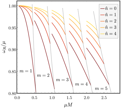
Figure 1: The harmonic part $\omega_{R}$ of the Proca frequency, as a function of Proca mass parameter $\mu M$ on a Kerr background with $a=0.99M$. For each $m$ mode, the first few overtones $\hat{n}$ are depicted for $S=-1$ (i.e., fastest growing) polarization state. The gray dashed lines indicate when the mode reaches saturation.

The real parts of the frequencies of oscillation $\omega_{R}$ are presented in Fig. 1. As can be seen there, there exists a clear hierarchical structure of the $\omega_{R}$ among the overtones for a given $m$: The real frequencies of the vector boson cloud are monotonically decrease with increasing overtone number $\hat{n}$. This is to be expected in the non-relativistic limit, but it holds also in the relativistic regime. This ensures that the superradiance condition $\omega_{R}<m\Omega_{H}$, for a fixed $m$-field mode, restricts the higher overtones to saturate before the lower ones.

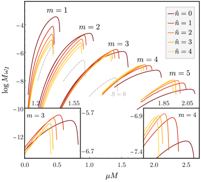
Figure 2: The growth rates of the dominant polarization state, $S=-1$, of the cloud for each $m$-mode over a range of Proca masses $\mu$. We assume the Kerr parameter $a=0.99M$, and include the first four overtones $\hat{n}$, as well as the fastest growing mode for the subleading polarization state $S=0$ (gray dashed line).

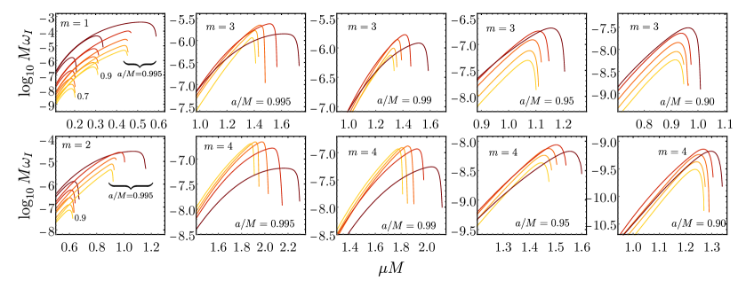
Figure 3: The growth rates of the first five overtones ($\hat{n}=0$, …, 4) of each $m$-field mode in the relevant Proca mass $\mu M$ range, and for several different dimensionless spin parameters $a/M$. For a description of the color-coding of the overtones see Fig. 2.

Figure 2 shows the instability growth rates for the fundamental field mode in the $S=-1$ polarization state, as well as several overtones, for different values of $m$. As already pointed out in Ref. Dolan (2018), the $S\in\{0,+1\}$ polarization states grow more slowly due to the fact that they are spatially concentrated farther from the BH horizon (and therefore from the source of energy and angular momentum). This example with $a=0.99M$ is typical of the behavior found for lower and higher Kerr spin parameters. The first two azimuthal Proca modes, $m=1$ and 2, have a strict hierarchical structure for this spin. The zeroth overtone, $\hat{n}=0$, is the most dominant, whereas with increasing overtone number $\hat{n}$, the instability growth rate decreases. Already in the $m=2$ case, the first signs of a switching of the most dominant mode between the overtones is noticeable. This effect of “overtone mixing” becomes more pronounced with increasing azimuthal number. In the $m=4$ case, for instance, the zeroth overtone is, in fact, the slowest growing mode out of the first five overtones. The hierarchy changes significantly with $\mu M$ and with spin parameter $a$. This overtone mixing behavior is captured by Fig. 3 for several different BH spins. The hierarchical structure of the $m=1$ overtones is preserved for all spin parameters $a\leq 0.995M$. However, already in the $m=2$ case, the fundamental mode ($\hat{n}=0$) mixes with the first overtone for BHs with near-extremal spin, with $\omega_{I}^{\hat{n}=1}>\omega_{I}^{\hat{n}=0}$ for certain choices of $\mu M$. For $m\geq 3$, the clear structure in the overtones is spoiled even for only moderately high spins. The fundamental mode tends to be subdominant at least in parts of the relevant Proca mass parameter range. Importantly, however, the $\hat{n}=0$ mode remains superradiant the furthest into the large $\mu M$-regime. This ensures that it is the last mode to reach saturation of the superradiance condition, and it can therefore grow significantly after the more dominant overtones have already reached saturation. Again, this is most pronounced around rapidly spinning BHs. It allows for the population of several different Proca field modes with significant amount of energy and angular momentum, and ultimately leads to beating GW signals, as each such populated Proca field mode has a slightly different real frequency $\omega_{R}$; we discuss this further in Secs. II.6 and IV.2.

Based on these data, we have constructed ready-to-use fit functions for the real and imaginary parts of the frequency for the most dominant unstable overtones for $m=1$, 2, and 3 (and $\hat{n}=0$). We employ a fitting function similar to that used in Ref. Cardoso et al. (2018), with a few modifications, achieving more accurate fits to the growth rates. Details on the fits and their accuracy can be found in the Appendix.

II.5 Evolution of instability and normalization

The initial conditions for the evolution of the cloud from an initial seed field configuration, to the macroscopic cloud, is, at the linear level, equivalent to an energy distribution across the different available modes. This includes (for a bound system) exponentially growing, as well as decaying, modes that could, in principle, carry different angular momenta. The choice of the angular momentum and mass distribution across the modes at the onset of the instability affects the final state of the system (see Ref. Ficarra et al. (2019) for an analysis of multi-mode initial conditions for a scalar cloud). Here we assume that: (i) the instability starts from a single vector boson in each unstable mode, (ii) the BH evolution is adiabatic and can be described as a sequence of Kerr spacetimes, (iii) the GW emission to infinity and across the horizon is neglected during the growth of the cloud, and finally, (iv) any additional matter accretion of the BH is ignored. We justify these assumptions below.

The system evolves through $\sim 170$ e-folds, from a single boson to the saturated cloud, which leads to an sensitive exponential dependence of the mass per mode on the relative growth rates. Hence, as long as the initial seed field (i.e., energy distribution) at the onset of the instability is small (e.g., condition (i) is satisfied), the saturated state of the system is expected to be completely dominated by a single, fastest growing, Proca field mode (see Ref. Ficarra et al. (2019)). An exception to this, which we discuss in the next sub-section, is when a mode with a lower instability rate can continue to grow after the saturation of the fastest growing mode. Secondly, fully non-linear evolutions of the set of Einstein-Proca equations revealed that the adiabatic approximation (ii) models the dynamics of the cloud’s growth even far from the test-field limit East (2018); East and Pretorius (2017). Furthermore, there is a clear separation of the GW emission and superradiant growth timescales $\tau_{\text{GW}}\gg\tau_{\text{sup.}}$. This implies (iii), so GW emission by the cloud (to infinity or through the BH horizon) can be ignored during the exponential growth phase of the vector cloud. Finally, restriction (iv) is merely a simplification given the range of possible accretion rates and the fact that we do not want to make any assumptions about the coupling of the massive vector boson under consideration to the Standard Model.

As discussed in Sec. I, the ratio of the adiabatic change of a spinning BH’s mass $\delta M$ and angular momentum $\delta J$ due to the presence of a single field mode, with azimuthal number $m$ and frequency $\omega_{R}$, is given by

$$\delta J/\delta M=m/\omega_{R}\ .$$ (20)

The final BH mass $M_{f}=M_{0}+\delta M$ and angular momentum $J_{f}=J_{0}+\delta J$ at the saturation of the instability are therefore determined by solving for the value of $\delta M$ which gives the horizon frequency at which the superradiance shuts off:

$$\Omega_{H}(M_{f},J_{f})=\Omega_{H}(M_{0}+\delta M,J_{0}+m\delta M/\omega_{R})=\omega_{R}/m\ .$$ (21)

In the above, $\omega_{R}$ is implicitly also a function of $M_{f}$ and $J_{f}$, though the dependence on $J_{f}$ is small. The explicit expression for the horizon frequency is

$$\Omega_{H}(M,J)=\frac{J}{2M\left(M^{2}+\sqrt{M^{4}-J^{2}}\right)}\ .$$ (22)

In Eq. (10), we indicated that we are solving for each Proca field mode, characterized by the set of eigenvalues $\{\omega,\nu,m\}$, but we left the overall normalization unspecified. A physical normalization of the modes is achieved by choosing the value of $C^{\nu}_{m\omega}$ in Eq. (10) so that the energy of the field solution matches the prediction of the above established adiabatic approximation. The mass contained in the solution $A_{\mu}$ of the Proca field equation is, in Boyer-Lindquist coordinates, and using Eq. (5), given by

$$E_{A}=-\int T^{t}{}_{t}(A)\sqrt{-g}drd\theta d\phi\ ,$$ (23)

where $g$ is the determinant of the Kerr metric. Then, for instance, the normalization at the time of saturation follows immediately from requiring that $E_{A}=M_{0}-M_{f}$, assuming only a single mode is populated at the saturation of the instability.

Beyond this normalization at the time of saturation, the temporal dependencies of the BH mass $M$ and angular momentum $J$, as well as the Proca cloud mass $E_{A}$, in the adiabatic context, are given by

$$\dot{E}_{A}= \ 2\omega_{I}(M,J)E_{A},$$ (24)

$$\dot{M}= \ -\dot{E}_{A},\qquad\dot{J}=m\omega^{-1}_{R}(M,J)\dot{M},$$ (25)

when considering a single Proca field mode. Therefore, once a single mode is normalized at the time of saturation (when Eq. (21) is satisfied), the entire time dependence of the cloud’s mass is fixed by Eq. (24) to be primarily exponential in nature. The implicit dependence of $\omega$ on the BH mass and angular momentum only becomes important when the cloud acquires a significant amount of energy from the BH; this happens in the very last stages before saturation (due to Eq. (25)), and is, as noted above in (ii), well-modeled by the adiabatic approximation. The evolution of a two-mode cloud is discussed in detail in the following subsection.

II.6 Transitions between overtones

So far, we have assumed that a single mode dominates the Proca cloud formed through superradiance. In the case of $m=1$, the lowest overtone ($\hat{n}=0$) is associated with the largest growth rate $\omega_{I}^{\hat{n}=0}$ across parameter space, which justifies this assumption. However, as pointed out in Sec. II.4, for $m\geq 2$, overtones $\hat{n}\geq 1$ can be faster growing than the respective zeroth overtone $\hat{n}=0$ for specific choices of $\mu M$ and BH spin $a$ (see also Figure 2). Since, as shown in Fig. 1, the overtone frequencies $\omega_{R}$ increase monotonically with $\hat{n}$, higher overtones saturate before the lower ones, and leave spun-down BHs that are unstable against the subsequent growth of lower overtones. The transition from the higher to the lower overtones allows for several superradiant Proca field modes to be populated simultaneously.

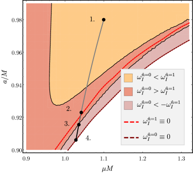
Figure 4: An illustration of which overtone of the $m=3$ Proca field mode has the dominant growth rate as a function of dimensionless BH spin $a/M$ and mass parameter $\mu M$. The dark gray and black lines show the evolution in BH mass and spin of an example BH-Proca system, as described in the text. The red dashed line is the saturation point of the $\hat{n}=1$ overtone, while the brown dashed line is the saturation point of the $\hat{n}=0$ overtone.

To illustrate this, let us consider a BH with initial mass $M_{0}$ and dimensionless spin $a_{0}/M_{0}=0.98$, as well as a Proca mass parameter $\mu M_{0}=1.1$. From Fig. 2, we can see that in this regime the $m=3$ field modes are the fastest growing, and that $\omega^{\hat{n}=1}_{I}>\omega^{\hat{n}=0}_{I}$ for the given initial BH parameters. The initial BH state corresponds to point 1. in Fig. 4. Due to the fact that $\omega_{I}^{\hat{n}=0}>\omega_{I}^{\hat{n}\geq 2}$ at point 1., we consider the $\hat{n}=0$ and $1$ modes only. Hence, the Proca cloud’s field solution is given by $A^{\text{cloud}}_{\mu}=A^{\hat{n}=1}_{\mu}+A^{\hat{n}=0}_{\mu}$ at any given time during the evolution of the instability. The energy momentum distribution is a sum of the energy momentum in $A^{\hat{n}=1}_{\mu}$ and $A^{\hat{n}=0}_{\mu}$, as well as a cross term $T_{\mu\nu}^{C}$ defined by

$$T_{\mu\nu}^{C}:=T_{\mu\nu}(A^{1}+A^{0})-T_{\mu\nu}(A^{1})-T_{\mu\nu}(A^{0}),$$ (26)

with $T_{\mu\nu}(A)$ given by Eq. (5), and where we have relaxed the notation: $A^{\hat{n}=i}_{\mu}\rightarrow A^{i}_{\mu}$. Then, the total mass of the two-mode cloud can be decomposed into $E_{A}^{\text{cloud}}=E_{A}^{1}+E_{A}^{0}+E_{A}^{C}$. The time dependence of each of the individual components of $E_{A}^{\text{cloud}}$ is taken to be of the exponential form of Eq. (24), with their associated growth rates $\omega_{I}$. We choose the initial conditions $E_{A}^{1}=E_{A}^{0}=m_{\gamma}$ to be the mass of a single vector boson (though the same behavior is expected from any sufficiently small initial field configuration). Due to the spatial overlap of $A^{1}_{\mu}$ and $A^{0}_{\mu}$, we find that $E_{A}^{C}\sim 0.01E_{A}^{1}$ at the onset of the instability. Starting with these initial data, the BH moves from 1. to 2. in Fig. 4 as the instability grows.

At point 2. in Fig. 4, the $\hat{n}=1$ mode saturates with $E_{A}^{1}\approx E_{A}^{\text{cloud}}=5.3\times 10^{-2}\ M_{0}$, where $E_{A}^{0}$ and $E_{A}^{C}$ are negligible, as shown in Fig. 5. At this stage in the process, $\omega_{I}^{\hat{n}=1}\approx 0$, while $\omega_{I}^{\hat{n}=0}>0$. Therefore, $E_{A}^{0}$ and $E_{A}^{C}$ continue growing, while $E_{A}^{1}$ stays roughly constant. As can be seen in Fig. 5, $E_{A}^{0}$ and $E_{A}^{C}$ grow until the BH approaches point 3. in Fig. 4, where the decay rate of the $\hat{n}=1$ mode (since its frequency is now above the threshold for superradiance) matches that of the growth rate of $\hat{n}=0$: $\omega^{\hat{n}=0}_{I}\approx|\omega_{I}^{\hat{n}=1}|$. Therefore, as the $\hat{n}=1$ mode falls back into the BH, the $\hat{n}=0$ mode keeps extracting energy and angular momentum from the BH. During this process, the spin and mass of the BH stay roughly constant. This is because, on the one hand, if the BH were to spin up due to the in-fall of $\hat{n}=1$, then the growth rate of $\hat{n}=0$ would increase and counter the increase in BH spin. On the other hand, if the BH is spun down significantly due to the growth of $\hat{n}=0$, then the decay rate of $\hat{n}=1$ dominates, and the spin-down process is damped. Therefore, the BH remains in the vicinity of point 3. throughout the entire transition period, where all but a negligible amount of energy is transferred from the $\hat{n}=1$ mode to the $\hat{n}=0$ overtone (see Fig. 5). As a consequence, while the BH stays at point 3., both the $\hat{n}=1$ and the $\hat{n}=0$ overtones are populated and carry significant fractions of the initial BH mass. This will lead to a a beating GW signal which we discuss in detail in Sec. IV.2. Finally, once the mass in the $\hat{n}=1$ mode becomes negligible, the zeroth overtone will spin down the BH further, until it reaches saturation at point 4.

Figure 5: The evolution of the components of the energy in a $m=3$ Proca cloud corresponding to the three terms in Eq. (26) for the example outlined in the text and Fig. 4. Time $t$ is shown in terms of $T_{s}$ (the time it takes for the $\hat{n}=1$ overtone to saturate); in this case, $T_{s}=0.51(M_{0}/M_{\odot})[1+0.012\log(M_{0}/M_{\odot})]$ hours. The gray band, bounded by gray dashed lines, indicates the region from $E=5\times 10^{-3}M_{0}$ to $E=M_{0}$ (i.e., the regime where the terms contain significant fractions of the initial BH mass $M_{0}$).

Note that the results presented in Fig. 5 are based on assuming the adiabatic approximation, and analyzing the different exponential time-dependencies between points 1. through 4. Of course, a non-linear evolution of the initial data described above is expected to show a smoothing of the rough first approximation of the Proca cloud’s dynamics (see the non-linear study in Ref. Chesler and Lowe (2019) for similar behavior in the context of the anti-de Sitter superradiant instability). Due to the exponential behavior, the dynamics of the instability is dominated only by the modes containing a significant fraction of the BH mass, and therefore the smoothing is expected to happen only very close to the individual points 2. through 4. For instance, the $E_{A}^{1}$ term will hardly decrease between points 2. and 3., since $E_{A}^{0}$ is still negligibly small, and only takes on significant values close to point 3. Hence, the location and length of 3. in Fig. 5, is subject to the somewhat arbitrary cutoff of when a mode is considered to contain a “significant” amount of energy (we used a cutoff of $E=5\times 10^{-3}M_{0}$). However, other reasonable choices of this cutoff will not affect the qualitative picture.

These types of transitions from higher to lower overtones for a given azimuthal mode number $m$ can be expected for all BHs with reasonably high spin and Proca masses that fall into the regime where $m\geq 3$ modes dominate the superradiance instability. This can be seen from Fig. 2, which shows the mixing of the growth rates of different overtones, with $m\geq 3$, for the case of $a/M=0.99$. These can have astrophysical significance as the growth rates even for some of the $m\geq 5$ azimuthal modes are still well below the age of the Universe, even for supermassive BHs. We give a detailed analysis of the potential observability of these overtone transitions in Sec. IV.2.

III Linear gravitational perturbations

In the previous section, we solved the linear Proca field equations on a fixed Kerr spacetime. The energy momentum tensor of the oscillating Proca cloud resulting for superradiance will source GWs. In this section, we describe how we solve the linearized Einstein equations to obtain the amplitude, frequency, and angular dependence of this gravitational radiation.

III.1 Teukolsky formalism

We compute the gravitational radiation at future null infinity $\mathscr{J}^{+}$ using the Teukolsky formalism Teukolsky (1973), which describes linear perturbations of the Kerr background. The Newman-Penrose (NP) Weyl scalar $\Psi_{4}:=C_{\alpha\beta\gamma\delta}n^{\alpha}m^{*\beta}n^{\gamma}m^{*\delta}$, encoding the gravitational radiation at $\mathscr{J}^{+}$, is projected out of the Weyl tensor $C_{\alpha\beta\gamma\delta}$, with the Kinnersley null tetrad

$$\begin{aligned} n^{\mu}:=&\ \frac{1}{2\Sigma}(r^{2}+a^{2},-\Delta,0,a),\\ m^{\mu}:=&\ \frac{\rho^{*}}{\sqrt{2}}(ia\sin\theta,0,1,i\sin^{-1}\theta),\end{aligned}$$ (27)

where $\rho:=(r-ia\cos\theta)^{-1}$, $\Sigma=r^{2}+a^{2}\cos^{2}\theta$, and $\Delta=r^{2}-2Mr+a^{2}$ are the usual Boyer-Lindquist functions. The Teukolsky equation for linear perturbations in $\Psi_{4}$ decouple for $\Phi:=\rho^{-4}\Psi_{4}$ in terms of the eigenfunctions $\{e^{-i\tilde{\omega}t},e^{i\tilde{m}\phi},{}_{-2}\tilde{S}_{\ell\tilde{m}}(a\tilde{\omega};\theta)\}$. The $s=-2$ spin-weighted spheroidal harmonics are by definition solutions of the angular Teukolsky equation. Here, and in the following, we distinguish the eigenfunctions and eigenvalues of the Teukolsky equations from the ones for the Proca field equations by a tilde. The spin-weighted spheroidal harmonics are normalized to $2\pi$ over the 2-sphere

$$\int^{\pi}_{0}|{}_{-2}\tilde{S}_{\ell\tilde{m}}(\theta)|^{2}\sin\theta d\theta=1.$$ (28)

In the Schwarzschild limit, i.e., setting the oblateness to zero, $a\tilde{\omega}\rightarrow 0$, the eigenvalue ${}_{-2}A_{\ell\tilde{m}}$ corresponding to ${}_{-2}\tilde{S}_{\ell\tilde{m}}(\theta)$ (see Ref.Teukolsky (1973) for details) is given by ${}_{-2}A_{\ell\tilde{m}}(a\tilde{\omega}\rightarrow 0)=\ell(\ell+1)+2$. Note that $\ell\geq\max(|\tilde{m}|,2)$. The radial Teukolsky equation is explicitly given by

$$\begin{aligned} \Delta^{2}\frac{d}{dr}\left[\Delta^{-1}\frac{d\tilde{R}_{\ell\tilde{m}\tilde{\omega}}}{dr}\right]+V_{\ell\tilde{m}\tilde{\omega}}(r)\tilde{R}_{\ell\tilde{m}\tilde{\omega}}=\hat{T}_{\ell\tilde{m}\tilde{\omega}},\\ V_{\ell\tilde{m}\tilde{\omega}}(r)=\left[\frac{K^{2}+4i(r-M)K}{\Delta}+8i\tilde{\omega}r+{}_{-2}\lambda_{\ell\tilde{m}\tilde{\omega}}\right],\end{aligned}$$ (29)

where ${}_{-2}\lambda_{\ell\tilde{m}\tilde{\omega}}:={}_{-2}A_{\ell\tilde{m}}+a^{2}\tilde{\omega}^{2}-2a\tilde{m}\tilde{\omega}$. The functions $\hat{T}_{\ell\tilde{m}\tilde{\omega}}$ are the projection of the source function $\tilde{T}$ for the Teukolsky master equation onto the basis of eigenfunctions established above:

$$\hat{T}_{\ell\tilde{m}\tilde{\omega}}=4\int_{\mathbb{R}}\frac{dt}{\sqrt{2\pi}}\int_{S^{2}}d\Omega{}_{-2}\tilde{S}^{*}_{\ell\tilde{m}}(a\tilde{\omega};\theta)e^{i\tilde{\omega}t-i\tilde{m}\phi}\frac{\tilde{T}(t,r,\Omega)}{\rho^{5}\rho^{*}}.$$ (30)

Note that the spheroidal harmonics are real in the case considered, and $d\Omega:=\sin\theta d\theta d\phi$ is the usual $S^{2}$ measure. Finally, the effective source $\tilde{T}(t,r,\Omega)$ in this NP description is computed from the projections of the stress-energy tensor $T_{\text{nn}}:=T_{\mu\nu}n^{\mu}n^{\nu},T_{\bar{\text{m}}\text{n}}:=T_{\mu\nu}n^{\mu}\bar{m}^{\nu}$, and $T_{\bar{\text{m}}\bar{\text{m}}}:=T_{\mu\nu}\bar{m}^{\mu}\bar{m}^{\nu}$ as

$$\tilde{T}(t,r,\Omega)= -\frac{1}{2}\rho^{8}\bar{\rho}\hat{\mathcal{L}}_{-1}[\rho^{-4}\hat{\mathcal{L}}_{0}(\rho^{-2}\bar{\rho}^{-1}T_{\text{nn}})]$$

$$-\frac{1}{2\sqrt{2}}\rho^{8}\bar{\rho}\Delta^{2}\hat{\mathcal{L}}_{-1}[\rho^{-4}\bar{\rho}^{2}\hat{\mathcal{J}}_{+}(\rho^{-2}\bar{\rho}^{-2}\Delta^{-1}T_{\bar{\text{m}}\text{n}})]$$

$$-\frac{1}{4}\rho^{8}\bar{\rho}\Delta^{2}\hat{\mathcal{J}}_{+}[\rho^{-4}\hat{\mathcal{J}}_{+}(\rho^{-2}\bar{\rho}T_{\bar{\text{m}}\bar{\text{m}}})]$$

$$-\frac{1}{2\sqrt{2}}\rho^{8}\bar{\rho}\Delta^{2}\hat{\mathcal{J}}_{+}[\rho^{-4}\bar{\rho}^{2}\Delta^{-1}\hat{\mathcal{L}}_{-1}(\rho^{-2}\bar{\rho}^{-2}T_{\bar{\text{m}}\text{n}})].$$

The differential operators used here are

$$\hat{\mathcal{L}}_{s}:= \ \partial_{\theta}-i\sin^{-1}\theta\partial_{\phi}-ia\sin\theta\partial_{t}+s\cot\theta,$$ (31)

$$\hat{\mathcal{J}}_{+}:= \ \partial_{r}-\Delta^{-1}[(r^{2}+a^{2})\partial_{t}+a\partial_{\phi}]\ .$$ (32)

III.2 Green’s function

As outlined above, the solution $\Phi$ to the Teukolsky equation can be decomposed into the following eigenfunctions:

$$\Psi_{4}=\rho^{4}\sum_{\ell,\tilde{m}\in\mathcal{K}}\int_{\mathbb{R}}\frac{d\tilde{\omega}^{\prime}}{\sqrt{2\pi}}{}_{-2}\tilde{S}_{\ell\tilde{m}}(\theta)e^{-i\tilde{\omega}^{\prime}t+i\tilde{m}\phi}\tilde{R}_{\ell\tilde{m}\tilde{\omega}^{\prime}}(r),$$ (33)

where here, and in the following, we have defined $\sum_{\ell,\tilde{m}\in\mathcal{K}}:=\sum_{\tilde{m}=-\infty}^{\infty}\sum_{\ell=\max(|\tilde{m}|,|s|)}^{\infty}$. This requires the inhomogeneous solution $\tilde{R}_{\ell\tilde{m}\tilde{\omega}^{\prime}}(r)$ of the radial Teukolsky equation (29). Since the separated Teukolsky equations are of Sturm-Liouville type, we do this by constructing a Green’s function from a set of homogeneous solutions satisfying the considered boundary conditions. As usual, we focus on solutions that are purely ingoing at the horizon, and purely outgoing at infinity. Therefore, following Ref. Sasaki and Tagoshi (2003), we define the two sets of homogeneous solutions $\{\tilde{R}^{\text{in}}_{\ell\tilde{m}\tilde{\omega}}(r),\tilde{R}^{\text{out}}_{\ell\tilde{m}\tilde{\omega}}(r)\}$ by the boundary conditions

$$\tilde{R}^{\text{in}}_{\ell\tilde{m}\tilde{\omega}}(r)=\begin{cases}B^{\text{trans}}_{\ell\tilde{m}\tilde{\omega}}\Delta^{2}e^{-ikr_{*}},&r\rightarrow r_{+}\\ B^{\text{refl}}_{\ell\tilde{m}\tilde{\omega}}r^{3}e^{i\tilde{\omega}r_{*}}+B^{\text{inc}}_{\ell\tilde{m}\tilde{\omega}}r^{-1}e^{-i\tilde{\omega}r_{*}},&r\rightarrow\infty\end{cases}$$ (34)

and

$$\tilde{R}^{\text{out}}_{\ell\tilde{m}\tilde{\omega}}(r)=\begin{cases}C^{\text{up}}_{\ell\tilde{m}\tilde{\omega}}r^{3}e^{ikr_{*}}+C^{\text{refl}}_{\ell\tilde{m}\tilde{\omega}}\Delta^{2}e^{-ikr_{*}},&r\rightarrow r_{+}\\ C^{\text{trans}}_{\ell\tilde{m}\tilde{\omega}}r^{3}e^{i\tilde{\omega}r_{*}},&r\rightarrow\infty\end{cases}$$ (35)

with $k:=\tilde{\omega}-\tilde{m}\Omega_{H}$. (Recall that $r_{*}$ is the radial tortoise coordinate defined in Eq. 19.) We obtain the homogeneous solutions using the MST formalism Mano et al. (1996); Sasaki and Tagoshi (2003); BHP . In this context, we find that the expansion of the homogeneous radial solution in terms of irregular confluent hypergeometric functions around $r\rightarrow\infty$ exhibits faster convergence behavior compared to the expansion around the horizon ($r=r_{+}$) in the part of the parameters space considered here. This is true even relatively close to the horizon. To check the validity of using the series expansion around $r\rightarrow\infty$ even close to the horizon, we compare the resulting solution with numerical integrations for the considered parameters and find good agreement.

From Sturm-Liouville theory, the general solution, provided any well-behaved source-function $\hat{T}_{\ell\tilde{m}\tilde{\omega}}$, is given by

$$\begin{aligned} \tilde{R}_{\ell\tilde{m}\tilde{\omega}}(r)=W_{\ell\tilde{m}\tilde{\omega}}^{-1}\Bigg{\{}&\ \tilde{R}_{\ell\tilde{m}\tilde{\omega}}^{\text{out}}\int_{r_{+}}^{r}dr^{\prime}\frac{\tilde{R}_{\ell\tilde{m}\tilde{\omega}}^{\text{in}}(r^{\prime})\hat{T}_{\ell\tilde{m}\tilde{\omega}}(r^{\prime})}{\Delta^{2}(r^{\prime})}\\ +&\ \tilde{R}_{\ell\tilde{m}\tilde{\omega}}^{\text{in}}\int_{r}^{\infty}dr^{\prime}\frac{\tilde{R}_{\ell\tilde{m}\tilde{\omega}}^{\text{out}}(r^{\prime})\hat{T}_{\ell\tilde{m}\tilde{\omega}}(r^{\prime})}{\Delta^{2}(r^{\prime})}\Bigg{\}},\end{aligned}$$ (36)

with the Wronskian $W_{\ell\tilde{m}\tilde{\omega}}:=(\tilde{R}^{\text{in}}_{\ell\tilde{m}\tilde{\omega}}\partial_{r}\tilde{R}^{\text{out}}_{\ell\tilde{m}\tilde{\omega}}-\tilde{R}^{\text{in}}_{\ell\tilde{m}\tilde{\omega}}\partial_{r}\tilde{R}^{\text{out}}_{\ell\tilde{m}\tilde{\omega}})/\Delta$. By virtue of the radial Teukolsky equation, $\partial_{r}W_{\ell\tilde{m}\tilde{\omega}}=0$. Combining this with the boundary conditions given by Eqs. (34) and (35) implies that the Wronskian is $W_{\ell\tilde{m}\tilde{\omega}}=2i\tilde{\omega}C_{\ell\tilde{m}\tilde{\omega}}^{\text{trans}}B_{\ell\tilde{m}\tilde{\omega}}^{\text{inc}}$. Therefore, the asymptotic solution at infinity is

$$\begin{aligned} \tilde{R}_{\ell\tilde{m}\tilde{\omega}}(r\rightarrow\infty)&=\frac{r^{3}e^{i\tilde{\omega}r_{*}}}{2i\tilde{\omega}B^{\text{inc}}_{\ell\tilde{m}\tilde{\omega}}}\int_{r_{+}}^{\infty}dr^{\prime}\frac{\hat{T}_{\ell\tilde{m}\tilde{\omega}}(r^{\prime})\tilde{R}_{\ell\tilde{m}\tilde{\omega}}^{\text{in}}(r^{\prime})}{\Delta^{2}(r^{\prime})}\\ &=:\tilde{Z}^{\infty}_{\ell\tilde{m}\tilde{\omega}}r^{3}e^{i\tilde{\omega}r_{*}}.\end{aligned}$$ (37)

While $\hat{T}_{\ell\tilde{m}\tilde{\omega}}$ has infinite support, the integral is well-defined due to the exponential decay of the Proca field for large $r$. Because of the symmetry relation $\tilde{Z}^{\infty}_{\ell,\tilde{m},\tilde{\omega}}=\tilde{Z}^{\infty*}_{\ell,-\tilde{m},-\tilde{\omega}}$, we need only focus on either positive-$\tilde{m}$ or negative-$\tilde{m}$ solutions.

Once the amplitude of the asymptotic solution $\tilde{R}_{\ell\tilde{m}\tilde{\omega}}(r\rightarrow\infty)$ to the inhomogeneous radial Teukolsky equation is found, the gravitational radiation at future null infinity $\mathscr{J}^{+}$ can be constructed. The Weyl-NP scalar at $\mathscr{J}^{+}$, $\Psi_{4}^{\infty}:=\lim_{r\rightarrow\infty}\Psi_{4}$, behaves like

$$\Psi_{4}^{\infty}(t,r,\theta,\phi)=\frac{1}{r}\sum_{\ell,\tilde{m}\in\mathcal{K}}\frac{\tilde{Z}^{\infty}_{\ell\tilde{m}\tilde{\omega}}}{\sqrt{2\pi}}e^{i\tilde{\omega}(r_{*}-t)+i\tilde{m}\phi}{}_{-2}\tilde{S}_{\ell\tilde{m}\tilde{\omega}}(\theta)\ ,$$ (38)

where we are focusing on a single frequency. We compute the GW radiation from the oscillations of different Proca modes (and ignoring any imaginary frequency component). Since the stress-energy is quadratic in the vector field, a single Proca mode with frequency $\omega_{R}$ and azimuthal number $m$ will source gravitational radiation with $|\tilde{m}|=2m$ and $\tilde{\omega}=2\omega_{R}$. (Hence $\tilde{\omega}$ can be considered to be implicitly labeled by the mode index $\tilde{m}$ and overtone number $\hat{n}$.)

III.3 Cloud dissipation and gravitational radiation

The evolution of the bosonic cloud can be split into two distinct phases, characterized by two different timescales. First, the cloud superradiantly grows in the unstable BH background with timescale $\tau_{\text{sup.}}=1/\omega_{I}$; second, the mass and angular momentum dissipate via GWs, characterized by the dissipation timescale $\tau_{\text{GW}}$. As already argued above, the separation of scales, $\tau_{\text{GW}}\gg\tau_{\text{sup.}}$, ensures that the GW dissipation can be neglected throughout the entire first phase of the cloud’s evolution. Additionally, the gravitational wave energy flux through the horizon is subdominant Poisson and Sasaki (1995), and hence will be neglected in what follows.

With these assumptions, we can formulate the evolution of the bosonic cloud during the dissipation process as: $\dot{E}_{A}=-\dot{E}_{\text{GW}}$. Here, $E_{A}(t)$ is the energy contained in the Proca cloud, whereas $\dot{E}_{\text{GW}}$ is the average GW flux to future null infinity. In the Teukolsky formalism described above, the GW energy flux averaged over several cloud oscillation periods is given by

$$\dot{E}_{\text{GW}}=\sum_{\ell,\tilde{m}\in\mathcal{K}}\frac{|\tilde{Z}^{\infty}_{\ell\tilde{m}\tilde{\omega}}|^{2}}{4\pi\tilde{\omega}^{2}}.$$ (39)

Since $\dot{E}_{\text{GW}}\propto|Z^{\infty}_{\ell\tilde{m}\tilde{\omega}}|^{2}\propto E_{A}(t)^{2}$, integrating in time gives

$$E_{A}(t)=\frac{E_{A}^{\text{sat.}}}{1+t/\tau_{\text{GW}}}, 1/\tau_{\text{GW}}:=\dot{E}_{\text{GW}}(t=0)/E_{A}^{\text{sat.}},$$ (40)

where $E_{A}(t=0)=E_{A}^{\text{sat.}}$ is the saturation energy of the cloud and we have defined the GW timescale $\tau_{\text{GW}}$ to be the time it takes for half of the initial saturation energy of the cloud to be radiated away.

In performing this calculation, we also have to specify the mass of the background geometry, i.e., the BH mass used when solving the Teukolsky equation, which should lie somewhere in the interval $(M_{f},M_{0})$, where $M_{f}$ is the BH mass at saturation. Towards the end of the dissipation phase, i.e., when the bosonic cloud is mostly dissipated and therefore has a small mass, the background BH has mass $M_{f}$ and angular momentum $J_{f}=a_{f}M_{f}$. The test field approximation of the Proca field is applicable and the cloud’s dynamics are well-modeled by a background geometry with parameters $M_{f}$ and $a_{f}$. On the other hand, the situation is not as clear at the onset of the dissipation. At that stage the BH-Proca system has mass $M_{0}$ and angular momentum $J_{0}=M_{0}a_{0}$, as the original BH. Hence, it can be expected that the energy contained in the Proca cloud affects the background geometry. This backreaction is not properly accounted for in our test field approximation. We can, however, approximate the combined BH-Proca configuration by a background Kerr geometry with unchanged mass and spin parameters $(M_{0},a_{0})$. This is what we do in the following, though we return to how the GW signal evolves with time in Sec. IV.3.

IV Results

Using the methods outlined in the previous section for solving the linearized Einstein equations, together with the Proca bound states obtained in Sec. II.4, we can compute the GW signals expected from ultralight vector boson clouds. In this section, we present results on the gravitational radiation expected from clouds populated by a single mode or multiple modes, and discuss the potential observability of such signals.

IV.1 Gravitational waves in the relativistic regime

We begin by comparing the GW energy flux we obtain with previous numerical and analytical results, as well as with the flux expected from an ultralight scalar boson cloud. In Fig. 6, we show a comparison for the case of a BH with spin $a/M=0.99$ and the $m=1$ ($\hat{n}=0$) Proca field mode. Note that we have normalized the GW flux by the cloud energy $E_{A}$ so as to be independent of this quantity in the test-field limit: $\dot{\tilde{E}}_{GW}:=\dot{E}_{GW}M^{2}/E_{A}^{2}$. Our relativistic results match those obtained in Ref. East (2017) using time-domain simulations, to within the estimated numerical error from the latter. This also matches the full general relativity results for the GW luminosity from the Proca cloud at saturation for $\mu M=0.4$ from Ref. East (2018).

In Fig. 6, we show two analytic approximations of the GW flux expected in the non-relativistic limit from Ref. Baryakhtar et al. (2017). Both are based on the same bound Proca field states obtained in the long-wavelength regime, where the massive wave equation in Kerr reduces to a set of Schrödinger equations. In the flat approximation, the flat d’Alembert Green’s functions were used to propagate the GWs from the source to null infinity. However, even the leading order GW flux in the non-relativistic limit is affected by the curved spacetime, so Ref. Baryakhtar et al. (2017) also calculated an approximation of the corrections from a Schwarzschild geometry (also shown). The actual GW flux in the non-relativistic limit is expected to fall in between these values, which is consistent with our results. In particular, as can be see from Figure 6, both the two small $\mu M$ approximations and our results follow the same powerlike behavior for $\mu M\lesssim 0.15$. However, when fitting $\beta\mu^{10}M^{10}$ to our numerical results in $0.065<\mu M<0.105$, we obtain a leading coefficient of $\beta=16.66$, while $\beta_{\text{flat}}=32/5$ and $\beta_{\text{Schw.}}=60$ for the flat and Schwarzschild approximation, respectively. Therefore, we further improve on the non-relativistic limit here, by reducing the order-of-magnitude uncertainty of the analytic results for $\mu M\ll 1$. Finally, for comparison, we also include the corresponding GW energy flux for a scalar boson cloud around a Kerr BH Yoshino and Kodama (2014); Brito et al. (2017b). Note that the scalar field mode saturates at smaller $\mu M$, compared to the vector field mode. Roughly speaking, the scalar GW power is six orders of magnitude smaller than the vector GW power.

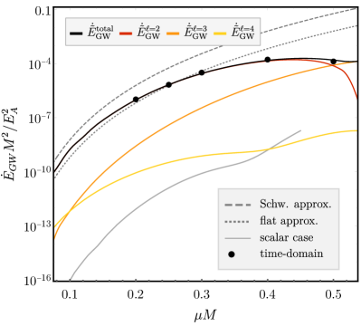
Figure 6: The GW flux of the $m=1$ (and $\hat{n}=0$) Proca field mode around a Kerr BH with spin parameter $a/M=0.99$. We show both the total GW flux $\dot{\tilde{E}}^{\text{total}}_{\text{GW}}$, and the individual contributions from spin-weighted spheroidal components with different angular numbers $\ell$ (see Eq. (39)). For comparison we show the results from time-domain simulations in the Proca-test field limit from Ref. East (2017) and the non-relativistic Schwarzschild and flatspace approximations from Ref. Baryakhtar et al. (2017). Finally, we compare these vector boson results to the GW energy flux from a scalar boson cloud presented in Refs. Brito et al. (2017b); Yoshino and Kodama (2014).

In our calculations of the GW energy flux, the dominant source of error emerges from inaccuracies in calculating the Proca field solutions with the appropriate boundary conditions. As discuss in Sec. II.3, the boundary condition for a bound Proca mode solution is enforced by minimizing the radial solution evaluated at large $r$ over the complex frequency plane. The more accurately the real and imaginary components of the frequency $\omega=\omega_{R}+i\omega_{I}$ are known, the larger the accuracy of the Proca field solutions. However, since we consider real frequencies with $\omega_{R}M\gtrsim 10^{-2}$, but growth rates as low as $\omega_{I}M\sim\mathcal{O}(10^{-10})$, the minimization over the complex $\omega$-plane is limited by the precision of the floating-point calculation. Therefore, we find that in the non-relativistic limit, i.e., in the limit of small growth rate, the Proca field solutions have larger relative uncertainties, which translates into less accurate GW energy flux results in that limit. For instance, the total GW energy flux of the $m=1$ mode, presented in Fig. 6, cannot be determined numerically with our approach for $\mu M<0.15$ without making use of higher than double precision. As a result of the decreasing maximal growth rate (with increasing azimuthal number $m$), the GW energy flux from higher-$m$ Proca field modes are less accurate. We estimate the numerical error by varying the precision cutoff of the minimization algorithm for the Proca field solutions and observing the convergence of the resulting GW energy flux. Based on this, the relative uncertainty of the $m=1$ GW power is $\lesssim 0.1\%$ for $\mu M\in(0.4,0.6)$, $\lesssim 1\%$ for $\mu M\in(0.2,0.4)$, and $\lesssim 5\%$ for $\mu M\in(0.065,0.2)$.

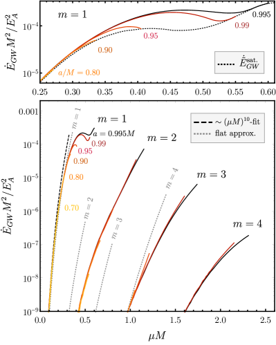
Figure 7: The total rescaled GW energy flux $\dot{E}_{\text{GW}}\times(M/E_{A})^{2}$ emitted by a Proca cloud (solid lines) in the fundamental mode ($\hat{n}=0$) for $m=1$, 2, 3, and 4. We show results from BHs with spin $a/M\in\{0.7,0.8,0.9,0.95,0.99,0.995\}$. In the bottom panel, we also show the fit we obtained in the text and compare to the flat approximation of Ref. Baryakhtar et al. (2017). The relativistic features of the GW power from a Proca cloud in the $m=1$ field mode are shown in more detail in the top panel, together with the mass-rescaled GW energy flux $\dot{\tilde{E}}^{\text{sat.}}_{GW}$ from a cloud that saturates the superradiant condition, i.e. with $\omega_{R}=\Omega_{H}$.

In Fig. 7, we present the GW power for different BH spins and azimuthal Proca field modes. The energy flux is insensitive to the dimensionless BH spin, except for near-extremal spins and large values of $\mu M$, where some differences can be seen for the $m=1$ mode (though the GW power from $m>1$ modes do not seem to share this behavior). In the top panel of Fig. 7, we also show the GW energy flux $\dot{\tilde{E}}^{\text{sat.}}_{GW}$ when the cloud frequency matches the BH rotational frequency $\omega_{R}=m\Omega_{H}$, as occurs at the saturation of the superradiant instability. This assumption sets the BH spin, and determines the features of the GW power in the relativistic regime. From these results, it is clear that the flat approximation Baryakhtar et al. (2017) significantly overestimates the GW power in the relativistic regime. Similarly to the $m=1$ case, we estimate the relative uncertainties of the $m=2$ result to be $\lesssim 1\%$ for $\mu M\in(0.7,1.2)$ and $\lesssim 5\%$ in the range $\mu M\in(0.45,0.7)$. In the $m=3$ case, we estimate the uncertainty to be $\lesssim 0.4\%$ for $\mu M\in(1.3,1.6)$ and $\lesssim 3\%$ for $\mu M\in(0.9,1.3)$. Finally, the relative uncertainties of our GW power results for a Proca cloud in the $m=4$ mode are $\lesssim 5\%$ for $\mu M\in(1.9,2.3)$ and $\lesssim 10\%$ for $\mu M\in(1.6,1.9)$.

In addition, we calculate the GW power from vector boson clouds in excited states for a BH spin of $a/M=0.99$ in Fig. 8. These indicate that the clouds in excited states with larger growth rates also emit stronger gravitational radiation compared to the fundamental modes. We also show the GW power associated with the beating oscillations due to two modes being simultaneously populated, which we discuss further in the next section.

IV.2 Gravitational waves from overtone transitions

As we have seen in Sec. II.6, there are parts of the BH-Proca parameter space where several different overtones of a given azimuthal mode number $m$ can be simultaneously populated. We continue the discussion of the example from Sec. II.6 here, and calculate the GW signal produced during the transition of the cloud from overtone to fundamental mode.

When the $\hat{n}=1$ overtone mode reaches saturation (point 2. in Fig. 4), its energy is $E_{A}^{1}=5.3\times 10^{-2}M_{0}$, while the contributions from the fundamental mode are negligible. Hence, the GWs are initially monochromatic with frequency given by $2\omega^{\hat{n}=1}_{R}\big{|}_{\textit{2.}}=2.10/M_{0}$. Since the GW emission timescale for the $\hat{n}=1$ overtone is much larger than the growth timescale of the $\hat{n}=0$ overtone (as already alluded to in Sec. II.6), the GW emission has no significant effect the cloud’s dynamics.

	$m_{\gamma}$ (eV)	$M_{0}$ ($M_{\odot}$)	$T_{\textit{1.}\rightarrow\textit{2.}}$	$T_{\textit{2.}\rightarrow\textit{3.}}$	$f^{\text{GW}}_{\textit{2.}\rightarrow\textit{3.}}$ (Hz)	$T_{\textit{3.}}$	$f^{\text{GW}}_{+}$ (Hz)	$f^{\text{GW}}_{-}$ (Hz)	$T_{\textit{3.}\rightarrow\textit{4.}}$	$f^{\text{GW}}_{\textit{3.}\rightarrow\textit{4.}}$ (Hz)
LIGO	$1\times 10^{-11}$	$92$	49.7 hours	$21.6$ hours	$731$	$2.7$ hours	$725$	$10.8$	$36$ min.	$714$
LISA	$5\times 10^{-17}$	$1.8\times 10^{7}$	1290 years	$567$ years	$3.66\times 10^{-3}$	$59$ years	$3.62\times 10^{-3}$	$5.38\times 10^{-5}$	$13.6$ years	$3.57\times 10^{-3}$

Table 1: The duration and associated GW frequencies of the stages where different overtones are populated for the example discussed in the text with $\mu M_{0}=1.1$ and $a_{0}/M_{0}=0.98$. We make two different choices for the physical mass of the vector boson $m_{\gamma}$ (from which the initial BH mass $M_{0}$ and all other quantities follow) corresponding to the LIGO and LISA bands. The quantity $T_{\textit{1.}\rightarrow\textit{2.}}$ is the time for the BH to evolve from point 1. to 2. in Fig. 4 (i.e. for the saturation of the $\hat{n}=1$ mode), and similarly for the other times. The different quantities $f_{\text{GW}}$ are the frequencies of the GWs emitted during the respective periods of time. In particular, we denote the GW frequencies associated to $\omega^{\hat{n}=1}_{R}-\omega^{\hat{n}=0}_{R}$ and $\omega^{\hat{n}=1}_{R}+\omega^{\hat{n}=0}_{R}$ with $f^{\text{GW}}_{-}$ and $f^{GW}_{+}$, respectively.

At $t\approx 1.44T_{s}$, where we recall that for this example $T_{s}=0.51(M_{0}/M_{\odot})[1+0.012\log(M_{0}/M_{\odot})]$ hours, the fundamental ($\hat{n}=0$) mode reaches one-tenth the energy of the $\hat{n}=1$ mode (approaching point 3. in Fig. 5). From Fig. 1, we see that the harmonic frequencies of the overtones $\hat{n}=1$ and $\hat{n}=0$ are different. Hence, the system, now consisting of two different field modes, emits gravitational radiation at the four different frequencies

$$\begin{aligned} 2\omega^{\hat{n}=1}_{R}M_{0}=&\ 2.10,\qquad&\ \omega_{+}M_{0}=2.07,\\ \omega_{-}M_{0}=&\ 0.03,\qquad&\ 2\omega^{\hat{n}=0}_{R}M_{0}=2.04,\end{aligned}$$ (41)

where we have defined $\omega_{+}:=\omega^{\hat{n}=1}_{R}+\omega^{\hat{n}=0}_{R}$ and $\omega_{-}:=\omega^{\hat{n}=1}_{R}-\omega^{\hat{n}=0}_{R}$. We illustrate how these frequencies and associated timescales would translate into physical units in Table 1, for two different choices of the vector boson mass that roughly correspond to the LIGO and LISA bands, respectively.

Fig. 8 shows the mass-rescaled GW energy fluxes, i.e., considering that $\dot{E}_{\text{GW}}^{\pm}\propto E_{A}^{1}E_{A}^{0}$, in the four different frequency components for the special case of $a=0.99M$ as a function of Proca mass. From this it is clear that the $\omega_{+}$ component has the most normalized power, with $\dot{\tilde{E}}^{+}_{\text{GW}}/\dot{\tilde{E}}_{\text{GW}}^{i}\sim\mathcal{O}(10^{1})$ (where $i\in\{0,1\}$), while $\dot{\tilde{E}}^{-}_{GW}$ is the weakest of the four.

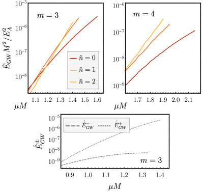
Figure 8: The total rescaled GW energy flux $\dot{E}_{\text{GW}}\times(M/E_{A})^{2}$ emitted by a Proca cloud in the fundamental mode ($\hat{n}=0$) and the first two excited states, $\hat{n}=1$ and 2, for $m=3$ (top-left panel) and $m=4$ (top-right panel) and BH spin $a=0.99M$. In the bottom panel we show the mass-rescaled GW energy fluxes $\dot{\tilde{E}}^{\pm}_{GW}=\dot{E}^{\pm}_{GW}M^{2}/(E^{1}_{A}E^{0}_{A})$ in the $\omega_{\pm}$ frequency components [as discussed below Eq. (41)] with BH spin $a=0.99M$.

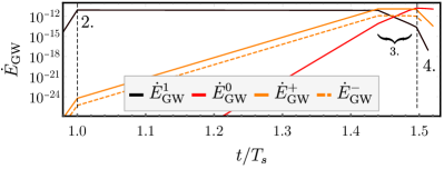
Figure 9: The GW energy flux $\dot{E}_{\text{GW}}$ emitted during the overtone transition from $\hat{n}=1$ to $\hat{n}=0$ of the $m=3$ azimuthal Proca field mode for the example presented in Sec. II.6. Here, $\dot{E}_{\text{GW}}^{i}$, with $i\in\{0,1\}$, corresponds to the frequencies $2\omega_{R}^{\hat{n}=i}$, while $\dot{E}^{\pm}_{\text{GW}}$ are associated with the frequencies $\omega_{\pm}$ (see Eq. (41)).

Specifically for this example, we show the GW power $\dot{E}_{\text{GW}}$ in each of these frequency channels before, during, and after the overtone transition in Fig. 9. Here, we are taking into account the distribution of energy across the two overtones (as opposed to scaling out the dependence on the cloud mass). Note that, since we are using the simple approximation of the evolution of the Proca cloud energy discussed in Sec. II.6, the total power of the GW signal, illustrated in Fig. 9, does not change smoothly in time. However, as discussed in Sec. II.6, we expect that a fully non-linear study of the mode transitions would reveal a smooth translation from the single-frequency GW signal into the multi-frequency phase, and finally back to the single-frequency GWs, until the cloud reaches saturation of the fundamental mode. In Fig. 9, we see that during the beating phase of the emitted gravitational radiation (while the BH-Proca system remains at point 3.), the frequency $\omega_{+}$ dominates the signal, while $2\omega^{\hat{n}=1}_{R}$ slowly fades out and $2\omega^{\hat{n}=0}_{R}$ gains in amplitude. The energy flux in the $\omega_{-}$ channel remains constant throughout the transition phase, just as the GW associated with $\omega_{+}$. However, the former is weaker than the latter, since $\dot{\tilde{E}}_{GW}^{-}\sim\dot{\tilde{E}}_{GW}^{i}$ in the relevant $\mu M$-range (see Figure 8). The overall GW power increase from 2. over 3. to 4. This is due to the fact that, at their respective saturation points, the $\hat{n}=0$ mode carries more energy compared with the $\hat{n}=1$ mode.

IV.3 GW frequency and drift

We now elaborate on the GW signals discussed in this section, and how they might fall into frequency ranges observable by ground-based GW detectors like LIGO for specific choices of boson mass and BH mass and spin. (Our results can be similarly applied to future space-based GW detectors like LISA by considering lower-mass bosons and supermassive BHs.)

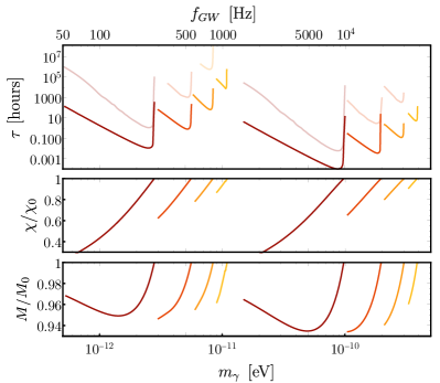
Figure 10: Using the estimated values for the properties of the BHs produced from the merger events GW170729 (left) and GW170817 (right) as initial conditions for the superradiant instability, we present here the final BH parameters, $M$ and dimensionless spin $\chi$, in terms of initial mass $M_{0}$ and spin $\chi_{0}=J_{0}/M_{0}^{2}$ as a function of GW frequency $f_{\rm GW}$ and Proca mass $m_{\gamma}$. In the top panel, we show both the superradiance timescale and the GW timescale (where, for a given mode, the latter is the longer timescale) for each of the Proca field modes $m=1,\ \dots,\ 4$ ($m=1$ in dark red, up to $m=4$ in light yellow), with $\hat{n}=0$. Note that, when constructing the top and bottom $x$-axis scales, we have approximated $\omega_{R}\approx\mu$. We omit the GW timescales for radiation from Proca clouds in the $m=4$ mode due to the larger numerical noise in the non-relativistic limit of our result (see Sec. IV.1).

When a binary BH merger takes place, it creates a newly formed spinning BH which, in the presence of an ultralight boson, is susceptible to the superradiant instability, and could thus give rise to GWs from the resulting boson cloud. In Fig. 10, we illustrate the expected properties for two LIGO merger events on the high and low end of the remnant mass. The first is GW170729, which gave rise to a BH with an estimated mass of $M_{0}=80\ M_{\odot}$ and dimensionless spin $\chi_{0}=0.81$ Abbott et al. (2019). The second is the neutron star merger GW170817, which we assume gave rise to a BH with $M_{0}=2.8\ M_{\odot}$ and $\chi_{0}=0.89$ (the upper end of the allowed range) Abbott et al. (2019), and ignore any possible effects from matter remaining outside the BH, for the purpose of this illustration. For the larger remnant mass case (GW170729), we can see in particular that the GWs fall into the range of LIGO’s sensitivity (roughly 10 Hz to a few kHz) for a sizable range of possible vector masses. In many cases in this range, a few percent of the BH’s total mass will be converted into a boson cloud, and ultimately radiated as GWs, on timescales that can be as short as hours. For the small remnant mass (GW170817), larger putative boson masses are probed, resulting in timescales that are even shorter (as short as minutes) and GW frequencies that are higher, typically above a kHz, where LIGO is less sensitive. Other remnant BHs with masses in between $3M_{\odot}$ and $80\ M_{\odot}$ will have properties intermediate to these two cases.

So far we have assumed that the GWs from boson clouds (at least those dominated by a single Proca mode) have constant frequency. However, there will be a small increase in the GW frequency as the mass of the BH-Proca cloud system decreases, due to the conversion of the cloud into GWs. Roughly speaking, the negative contribution to a boson’s energy, and hence frequency, due to the self-gravity of the cloud decreases, leading to higher frequency gravitational radiation. This frequency drift can be important for continuous GW searches, and can limit the range of accessible sources when not taken into account, especially for GWs from massive vector clouds (as opposed to massive scalar clouds), due to their small GW timescales (and therefore, larger frequency derivatives). We note that this positive frequency derivative of the (almost) monochromatic GW signal stands in contrast to the negative frequency derivative expected, for example, in a pulsar spinning down due to GW emission from a mountain.

As a first estimate of the expected change in GW frequency during the evolution and eventual dissipation of a Proca cloud, we compute the difference in frequency $\Delta f$ between the GWs obtained when solving on a BH background with the original mass $M_{0}$ and spin $a_{0}$, and those obtained on a BH background with mass decreased by half the saturation energy of the boson cloud $M=M_{0}-E_{A}^{\text{sat.}}/2$ and an equivalently lower spin $a$ (as obtained through Eq. (20)). This is shown in Fig. 11 (labeled as “BH limit”). Note that the real part of the frequency is hardly dependent on the dimensionless background spin, making the decrease in mass of BH-Proca system the leading contribution to the frequency drift. This BH perturbation theory calculation of course ignores the fact that during the GW emission phase, some of the mass of the system is spread over the spatial extent of the cloud (as opposed to all being in the BH), and thus overestimates the magnitude of the gravitational self-energy of the cloud. In Ref. Baryakhtar et al. (2017), the frequency drift was estimated in the non-relativistic limit using the Newtonian expression for the gravitational self-energy of the cloud. For comparison, we also show their result in Fig. 11, as well as the estimate we obtain using our relativistic expression for the cloud energy density and cloud saturation energy $E_{A}$ in a similar calculation.

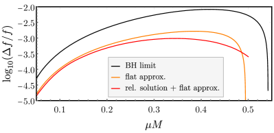
Figure 11: The total relative frequency drift $\Delta f/f$ a monochromatic GW signal experiences during the first GW timescale $\tau_{\text{GW}}$ after saturation of the superradiant instability of the $m=1$ Proca field mode around a BH with $a/M=0.99$. In our approach of estimating $\Delta f$, labeled “BH limit”, the spatial distribution of the cloud’s self-energy is ignored, instead, it is added to the BH mass. For comparison, we also show the non-relativistic results obtained in Ref. Baryakhtar et al. (2017) (labeled “flat approx.”), as well as a similar calculation using the same Newtonian expression for the cloud’s self gravity, but our relativistic expressions for the energy density and saturation energy (red line).

In Fig. 11, we consider a BH-Proca system with $a/M=0.99$ in the $m=1$ fundamental mode, though similarly large frequency changes occur also for the zeroth overtones of $m=2$, 3, and 4. In the non-relativistic limit, the BH limit calculation is larger by a factor of $\approx 3$ compared to the other calculations, just due to the fact that all the mass is assumed to be in the BH, which is only valid at early times, before the boson cloud as obtained significant mass, and at late times, after the boson cloud has mostly dissipated. For the other curves in Fig. 11, which make use of the Newtonian expression for the cloud’s self gravity, replacing the flat approximation of Ref. Baryakhtar et al. (2017) by our relativistic solutions of the Proca field gives a small difference (mainly due to the different values of $E_{A}^{\text{sat.}}$), and actually decreases the estimated frequency change (except at large values of $\mu M$).

V Discussion and Conclusion

We have investigated the superradiant instability of a massive vector field around a spinning BH with techniques from BH perturbation theory, and utilizing an adiabatic approximation to model the evolution of the BH and Proca cloud. We calculated the properties of the GWs that would be emitted by vector boson clouds that arise through superradiance, including their frequency, amplitude, and evolution.

We found that the quasi-normal bound states of a Proca field around a Kerr BH exhibit a rich overtone structure in the relativistic regime. Excited states ($\hat{n}>0$) of the Proca field can, depending on the Proca mass and BH spin, have the largest instability rate, and thus dominate the initial dynamics. Since lower-$\hat{n}$ states always have lower frequency, and thus can continue to grow after the saturation of higher frequency instabilities, this leads to overtone mixing. For $m=1$, the fundamental mode is the most unstable. However, for $m=2$, this overtone mixing occurs only for near-extremal BH spin, while for $m=3$, it occurs for moderately high BH spins. For $m\geq 4$ the overtone mixing occurs even in the non-relativistic limit, and would produce several overtone transitions. Similar overtone mixing in the relativistic regime was found in the scalar boson case for $m=3$ modes Yoshino and Kodama (2015).

After the saturation of the fastest growing overtone, the Proca cloud undergoes transitions between the excited states until the instability finally saturates in the fundamental mode. Several modes can be populated simultaneously during these overtone transitions, which, leads to a distinctive multi-frequency GW signature. As we have seen, the gravitational radiation in the transition phases is just as strong as during the monochromatic phases, and the frequencies could also fall into the LIGO/LISA bands. In fact, the beat frequency can be orders of magnitude smaller than the individual overtone frequencies, making signals from BH-Proca systems with heavier massive vector bosons fall into a detectable frequency range when the individual frequencies are too high frequency to detect. However, the amount of time spent in this phase (and thus total radiated energy) is small, making observing them more difficult. For the specific example discussed in Sec. IV.2, the transition phase lasts only $4\%$ of the time from the onset of the instability to the saturation of the zeroth overtone, and only $\approx 10^{-3}\tau_{\text{GW}}$ (the GW dissipation timescale of the cloud).

In this work, we calculated the power of the GW emission from Proca clouds around spinning BHs using the linearized Einstein equations, improving upon the flat and Schwarzschild approximations from Ref. Baryakhtar et al. (2017) in the non-relativistic limit. We also substantially expanded on the parameter space covered compared to the previous relativistic calculations in Refs. East (2017, 2018), studying a range of BH spins, different Proca field modes (azimuthal numbers $m=1$, 2, 3, and 4) and overtones ($\hat{n}\geq 0$). We find that the GW energy flux normalized by the cloud mass is mostly independent of the BH’s spin. Our results also show that the flat approximation significantly overestimates the energy flux from Proca clouds for larger values of $\mu M$ (and this appears to get worse for increase values of $m$). For $m=1$, and small (non-relativistic) values of $\mu$, the flat approximation underestimates the GW power by a factor of a few.

Our results can be used in searches for the GW signals from ultralight vector boson clouds around spinning BHs, which could fall into several different categories. First, targeted searches can be used to follow-up detections of compact binary mergers, where the remnant is a spinning BH Ghosh et al. (2019); Isi et al. (2019). Using the measured properties of the BH, these results can be used to predict the possible signals for different putative boson masses. In such targeted searches, the above described overtone transitions, and associated distinctive GW signatures, should also be taken into account. In addition, all-sky continuous GW searches Goncharov and Thrane (2018); D’Antonio et al. (2018), tailored to these sources, could provide more stringent bounds on vector boson masses, similar to the analysis in Ref. Palomba et al. (2019) for the scalar case. Finally, one can search for, or place constraints on, ultralight vector bosons by looking for a stochastic GW background, similarly to the scalar case Brito et al. (2017a, b).

Compared to ultralight scalars, vectors have a superradiance instability growth rate and GW amplitude that is several orders of magnitude larger. As we have seen here, the timescale for a vector boson cloud around a stellar mass BH to be converted into GWs can be as short as hours. Though the GW signal is louder, the shorter duration, as well as the faster frequency increase in the signal may be a challenge for conventional continuous GW searches, which typically assume a signal that lasts the duration of an observing run. This may be a motivation for designing intermediate timescale searches, as well as including an accurate description of the frequency evolution in a waveform model.

*

Appendix A Frequency fit functions

In this appendix, we present our fit functions, and their corresponding accuracy, for the real and imaginary parts of the frequency $\omega=\omega_{R}+i\omega_{I}$ of the superradiantly unstable Proca modes. These were obtained by fitting to the numerical data obtained in Sec.  II.4. We utilize the ansatz

$$\begin{aligned} \frac{\omega_{R}}{\mu}-1+\frac{\mu^{2}M^{2}}{2m^{2}}=&\ (\mu M)^{4}\hat{a}_{4,0,m}\\ &+\sum_{p\geq 5}\sum_{q\geq 0}(\mu M)^{p}\hat{a}_{p,q,m}(1-\chi^{2})^{q/2}\end{aligned}$$ (42)

for the real part, and

$$\begin{aligned} \frac{\omega_{I}M(\mu M)^{-3-4m}}{C_{m}f_{m}(\omega_{R}-m\Omega_{H})}-1=\sum_{p\geq 1}\sum_{q\geq 0}(\mu M)^{p}\big{[}\hat{b}_{p,q,m}\chi^{q+1}\\ \hskip 56.9055pt+\hat{c}_{p,q,m}(1-\chi^{2})^{q/2}\big{]},\end{aligned}$$ (43)

for the imaginary part. Here $C_{1}=2$, $C_{2}=1/1728$, $C_{3}=4/(199290375)$, and $f_{m}=\prod_{h=1}^{m}[h^{2}(1-\chi^{2})+(\chi m-2r_{+}\omega_{R})^{2}]$ Baumann et al. (2019b); Baryakhtar et al. (2017), while $\chi=a/M$. We present fit functions for the frequency of only the fundamental ($\hat{n}=0$) modes with $m=1$ through $m=3$, since these dominate the dynamics for the largest part of the parameter space. In Eqs. (42) and (43), we factor out the leading-order contributions in the non-relativistic limit of $\omega_{R}$ Baryakhtar et al. (2017). As discussed below, we have tested these fits only against our numerical results in the relativistic regime. However, we factored out the known non-relativistic corrections, and therefore expect those fits to also do well in the rest of the parameter space. Notice, though, that there is a $\mu M$ range between the regime in which we tested the fits and the non-relativistic limit, where the fits may behave differently from the true result. This matching range increases in size with increasing azimuthal mode number. The coefficients for the real parts of the frequencies are given in Table 2, whereas the coefficients for the imaginary parts are given in Table 3.

$\hat{a}_{p,q,1}$	$q=0$	$q=1$	$2$	$3$
$p=5$	-0.870039	1.92247	-6.93044	-0.651989
$6$	6.00734	-10.4118	30.3691	18.2029
$7$	-4.23715	11.2671	-33.6966	-102.444
$\hat{a}_{p,q,2}$	$q=0$	$q=1$	$2$	$3$
$p=5$	-0.00276306	0.025062	-0.164217	0.0216578
$6$	0.0380878	-0.0949728	0.458643	-0.00599547
$7$	-0.0093238	0.0654495	-0.333585	-0.26639
$\hat{a}_{p,q,3}$	$q=0$	$q=1$	$2$	$3$
$p=0$	-0.000649075	0.00748510	-0.0294351	0.00695179
$6$	0.00362974	-0.0131563	0.0434778	-0.000717772
$7$	-0.000682509	0.00508197	-0.0175571	-0.0139853

Table 2: The fit coefficients for the real part of the frequency, as defined in (42) and (43). Additionally, $\hat{a}_{4,0,1}=-1.16304$, $\hat{a}_{4,0,2}=-0.0614401$ and $\hat{a}_{4,0,3}=-0.0116139$.

$\hat{b}_{p,q,1}\times 10^{-5}$	$p=1$	$2$	$3$	$4$	$5$	$6$	$7$	$8$	$9$	$10$
$q=0$	-0.000172849	0.021852	-0.957118	19.2205	-189.031	794.509	319.628	-14176.	43620.8	-42174.6
$1$	-0.000058719	0.00396914	0.0401875	-3.77957	58.1935	-318.606	40.1126	5746.01	-19453.2	19763.2
$\hat{b}_{p,q,2}\times 10^{-5}$	$p=5$	$6$	$7$	$8$	$9$	$10$	$11$	$12$	$13$	$14$
$q=0$	14.4455	-235.964	1808.47	-8368.42	25191.5	-50221.	65445.7	-53266.5	24374.1	-4724.85
$1$	-10.1872	146.829	-999.726	4224.45	-12019.5	23314.2	-30142.	24612.9	-11363.4	2227.57
$\hat{b}_{p,q,3}$	$p=13$	$14$	$15$	$16$	$17$	$18$	$19$	$20$	$21$	$22$
$q=1$	15037.966	-7589.684	-11073.655	-3450.736	1195.4877	1572.5096	897.2985	820.2915	978.5094	472.0680
$2$	-17130.990	14309.731	5272.649	2467.256	1106.0694	-760.0280	-1706.9831	-1308.4764	-543.7076	-550.2190

$\hat{c}_{p,q,1}\times 10^{-5}$	$p=1$	$2$	$3$	$4$	$5$	$6$	$7$	$8$	$9$	$10$
$q=0$	0.000150374	-0.0236152	0.891463	-15.3662	131.805	-485.664	-321.996	8357.09	-24098.5	22385.9
$1$	0.0000910064	0.00369826	-0.207125	3.99915	-37.1508	186.221	-514.875	753.039	-504.345	103.496
$\hat{c}_{p,q,2}\times 10^{-5}$	$p=5$	$6$	$7$	$8$	$9$	$10$	$11$	$12$	$13$	$14$
$q=0$	-3.5933	80.1423	-756.209	3969.73	-12810.3	26419.5	-34878.1	28421.6	-12939.2	2487.81
$1$	-3.71268	47.4052	-258.085	782.508	-1441.81	1643.4	-1114.8	391.394	-37.5528	-8.74807
$\hat{c}_{p,q,3}$	$p=13$	$14$	$15$	$16$	$17$	$18$	$19$	$20$	$21$	$22$
$q=1$	0	-1060.1836	-3388.984	6247.957	1138.9217	-2112.0303	-2230.7653	4.619473	1812.5793	-599.9215
$2$	114566.94	-376625.9	396163.0	-55852.15	-120416.34	9180.998	45541.30	4094.197	-19781.675	4743.193

Table 3: The fit coefficients for the imaginary parts of the frequencies as defined in (42) and (43). Notice that we chose $\hat{b}_{p\leq 4,q,2}=\hat{c}_{p\leq 4,q,2}=0$, as well as $\hat{b}_{p\leq 12,q,3}=\hat{c}_{p\leq 12,q,3}=0$, to find a good match of the non-relativistic limit with our results.

We have compared the fit function for $m=1$ with our numerical data for the same frequencies in the regime $\mu M\in(0.05,(\mu M)_{\text{sat.}})$, where $(\mu M)_{\text{sat.}}$ is the saturation point for a given spin. In this regime, and for $a/M\in(0.4,0.99)$, we find a maximum relative residual, $x_{\text{max}}(\omega_{R,I}):=\max(|\omega_{R,I}^{\text{fit}}-\omega_{R,I}^{\text{numerical}}|/\omega_{R,I}^{\text{numerical}})$, in $\omega_{R}$ of $x_{\text{max}}^{\text{m=1}}(\omega_{R})=7.4\times 10^{-5}$, whereas the mean relative residual, $x_{\text{mean}}(\omega_{R,I}):=\text{mean}(|\omega_{R,I}^{\text{fit}}-\omega_{R,I}^{\text{numerical}}|/\omega_{R,I}^{\text{numerical}})$, over this part of the parameter space is $x_{\text{mean}}^{\text{m=1}}(\omega_{R})=2.4\times 10^{-6}$. Similarly, for $\omega_{I}$, the fit functions residual in the region $(\mu M,a)\in(0.05,(\mu M)_{\text{sat.}}),(0.4,0.99))$, is given by $x_{\text{max}}^{\text{m=1}}(\omega_{I})=9.7\times 10^{-3}$ and $x_{\text{mean}}^{\text{m=1}}(\omega_{I})=1.4\times 10^{-3}$. Beyond this regime, i.e., for smaller spins $a$, we have not tested this fit.

For the $m=2$ and $m=3$ frequencies, we compared the fit functions to our data in the regimes $(\mu M,a)_{m=2}\in((0.35,(\mu M)_{\text{sat.}}),(0.7,0.99))$ and $(\mu M,a)_{m=3}\in((0.8,(\mu M)_{\text{sat.}}),(0.8,0.99))$, respectively. In their respective regimes, we find the accuracy of the fits to be

$$\begin{aligned} x_{\text{max}}^{m=2}(\omega_{R})=&\ 6.9\times 10^{-5},\qquad&x_{\text{mean}}^{m=2}(\omega_{R})=7.5\times 10^{-6},\\ x_{\text{max}}^{m=2}(\omega_{I})=&\ 1.4\times 10^{-2},\qquad&x_{\text{mean}}^{m=2}(\omega_{I})=4.0\times 10^{-3},\end{aligned}$$

and

$$\begin{aligned} x_{\text{max}}^{m=3}(\omega_{R})=&\ 3.9\times 10^{-5},\qquad&x_{\text{mean}}^{m=3}(\omega_{R})=3.1\times 10^{-6},\\ x_{\text{max}}^{m=3}(\omega_{I})=&\ 3.1\times 10^{-1},\qquad&x_{\text{mean}}^{m=3}(\omega_{I})=2.5\times 10^{-2}.\end{aligned}$$

References

- Arvanitaki et al. (2010) A. Arvanitaki, S. Dimopoulos, S. Dubovsky, N. Kaloper, and J. March-Russell, Phys. Rev. D81, 123530 (2010), arXiv:0905.4720 [hep-th] .
- Jaeckel and Ringwald (2010) J. Jaeckel and A. Ringwald, Ann. Rev. Nucl. Part. Sci. 60, 405 (2010), arXiv:1002.0329 [hep-ph] .
- Arvanitaki and Dubovsky (2011) A. Arvanitaki and S. Dubovsky, Phys. Rev. D83, 044026 (2011), arXiv:1004.3558 [hep-th] .
- Agrawal et al. (2018) P. Agrawal, N. Kitajima, M. Reece, T. Sekiguchi, and F. Takahashi, (2018), arXiv:1810.07188 [hep-ph] .
- Essig et al. (2013) R. Essig et al., in Proceedings, 2013 Community Summer Study on the Future of U.S. Particle Physics: Snowmass on the Mississippi (CSS2013): Minneapolis, MN, USA, July 29-August 6, 2013 (2013) arXiv:1311.0029 [hep-ph] .
- De Felice et al. (2016a) A. De Felice, L. Heisenberg, R. Kase, S. Mukohyama, S. Tsujikawa, and Y.-l. Zhang, Phys. Rev. D94, 044024 (2016a), arXiv:1605.05066 [gr-qc] .
- De Felice et al. (2016b) A. De Felice, L. Heisenberg, R. Kase, S. Mukohyama, S. Tsujikawa, and Y.-l. Zhang, JCAP 1606, 048 (2016b), arXiv:1603.05806 [gr-qc] .
- Peccei and Quinn (1977) R. D. Peccei and H. R. Quinn, Phys. Rev. Lett. 38, 1440 (1977).
- Weinberg (1978) S. Weinberg, Phys. Rev. Lett. 40, 223 (1978).
- Abbott et al. (2016) B. P. Abbott et al. (LIGO Scientific, Virgo), Phys. Rev. Lett. 116, 241103 (2016), arXiv:1606.04855 [gr-qc] .
- Abbott et al. (2019) B. P. Abbott et al. (LIGO Scientific, Virgo), Phys. Rev. X9, 031040 (2019), arXiv:1811.12907 [astro-ph.HE] .
- Bardeen et al. (1973) J. M. Bardeen, B. Carter, and S. W. Hawking, Commun. Math. Phys. 31, 161 (1973).
- Press and Teukolsky (1972) W. H. Press and S. A. Teukolsky, Nature 238, 211 (1972).
- East (2018) W. E. East, Phys. Rev. Lett. 121, 131104 (2018), arXiv:1807.00043 [gr-qc] .
- East and Pretorius (2017) W. E. East and F. Pretorius, Phys. Rev. Lett. 119, 041101 (2017), arXiv:1704.04791 [gr-qc] .
- Davoudiasl and Denton (2019) H. Davoudiasl and P. B. Denton, (2019), arXiv:1904.09242 [astro-ph.CO] .
- Cardoso et al. (2018) V. Cardoso, O. J. C. Dias, G. S. Hartnett, M. Middleton, P. Pani, and J. E. Santos, JCAP 1803, 043 (2018), arXiv:1801.01420 [gr-qc] .
- Baumann et al. (2019a) D. Baumann, H. S. Chia, and R. A. Porto, Phys. Rev. D99, 044001 (2019a), arXiv:1804.03208 [gr-qc] .
- Berti et al. (2019) E. Berti, R. Brito, C. F. B. Macedo, G. Raposo, and J. L. Rosa, Phys. Rev. D99, 104039 (2019), arXiv:1904.03131 [gr-qc] .
- Zhang and Yang (2019a) J. Zhang and H. Yang, Phys. Rev. D99, 064018 (2019a), arXiv:1808.02905 [gr-qc] .
- Zhang and Yang (2019b) J. Zhang and H. Yang, (2019b), arXiv:1907.13582 [gr-qc] .
- Herdeiro et al. (2016) C. Herdeiro, E. Radu, and H. Rúnarsson, Class. Quant. Grav. 33, 154001 (2016), arXiv:1603.02687 [gr-qc] .
- Herdeiro and Radu (2017) C. A. R. Herdeiro and E. Radu, Phys. Rev. Lett. 119, 261101 (2017), arXiv:1706.06597 [gr-qc] .
- Ganchev and Santos (2018) B. Ganchev and J. E. Santos, Phys. Rev. Lett. 120, 171101 (2018), arXiv:1711.08464 [gr-qc] .
- Arvanitaki et al. (2015) A. Arvanitaki, M. Baryakhtar, and X. Huang, Phys. Rev. D91, 084011 (2015), arXiv:1411.2263 [hep-ph] .
- Arvanitaki et al. (2017) A. Arvanitaki, M. Baryakhtar, S. Dimopoulos, S. Dubovsky, and R. Lasenby, Phys. Rev. D95, 043001 (2017), arXiv:1604.03958 [hep-ph] .
- Tsukada et al. (2019) L. Tsukada, T. Callister, A. Matas, and P. Meyers, Phys. Rev. D99, 103015 (2019), arXiv:1812.09622 [astro-ph.HE] .
- Brito et al. (2017a) R. Brito, S. Ghosh, E. Barausse, E. Berti, V. Cardoso, I. Dvorkin, A. Klein, and P. Pani, Phys. Rev. Lett. 119, 131101 (2017a), arXiv:1706.05097 [gr-qc] .
- Brito et al. (2017b) R. Brito, S. Ghosh, E. Barausse, E. Berti, V. Cardoso, I. Dvorkin, A. Klein, and P. Pani, Phys. Rev. D96, 064050 (2017b), arXiv:1706.06311 [gr-qc] .
- Baryakhtar et al. (2017) M. Baryakhtar, R. Lasenby, and M. Teo, Phys. Rev. D96, 035019 (2017), arXiv:1704.05081 [hep-ph] .
- Baumann et al. (2019b) D. Baumann, H. S. Chia, J. Stout, and L. ter Haar, (2019b), arXiv:1908.10370 [gr-qc] .
- Pani et al. (2012) P. Pani, V. Cardoso, L. Gualtieri, E. Berti, and A. Ishibashi, Phys. Rev. D86, 104017 (2012), arXiv:1209.0773 [gr-qc] .
- Witek et al. (2013) H. Witek, V. Cardoso, A. Ishibashi, and U. Sperhake, Phys. Rev. D87, 043513 (2013), arXiv:1212.0551 [gr-qc] .
- East (2017) W. E. East, Phys. Rev. D96, 024004 (2017), arXiv:1705.01544 [gr-qc] .
- Frolov et al. (2018) V. P. Frolov, P. Krtouš, D. Kubizňák, and J. E. Santos, Phys. Rev. Lett. 120, 231103 (2018), arXiv:1804.00030 [hep-th] .
- Lunin (2017) O. Lunin, JHEP 12, 138 (2017), arXiv:1708.06766 [hep-th] .
- Krtouš et al. (2018) P. Krtouš, V. P. Frolov, and D. Kubizňák, Nucl. Phys. B934, 7 (2018), arXiv:1803.02485 [hep-th] .
- Teukolsky (1973) S. A. Teukolsky, Astrophys. J. 185, 635 (1973).
- Press and Teukolsky (1973) W. H. Press and S. A. Teukolsky, Astrophys. J. 185, 649 (1973).
- Ficarra et al. (2019) G. Ficarra, P. Pani, and H. Witek, Phys. Rev. D99, 104019 (2019), arXiv:1812.02758 [gr-qc] .
- Dolan (2018) S. R. Dolan, Phys. Rev. D98, 104006 (2018), arXiv:1806.01604 [gr-qc] .
- Chesler and Lowe (2019) P. M. Chesler and D. A. Lowe, Phys. Rev. Lett. 122, 181101 (2019), arXiv:1801.09711 [gr-qc] .
- Sasaki and Tagoshi (2003) M. Sasaki and H. Tagoshi, Living Rev. Rel. 6, 6 (2003), arXiv:gr-qc/0306120 [gr-qc] .
- Mano et al. (1996) S. Mano, H. Suzuki, and E. Takasugi, Prog. Theor. Phys. 95, 1079 (1996), arXiv:gr-qc/9603020 [gr-qc] .
- (45) “Black Hole Perturbation Toolkit,” (bhptoolkit.org).
- Poisson and Sasaki (1995) E. Poisson and M. Sasaki, Phys. Rev. D51, 5753 (1995), arXiv:gr-qc/9412027 [gr-qc] .
- Yoshino and Kodama (2014) H. Yoshino and H. Kodama, PTEP 2014, 043E02 (2014), arXiv:1312.2326 [gr-qc] .
- Yoshino and Kodama (2015) H. Yoshino and H. Kodama, Class. Quant. Grav. 32, 214001 (2015), arXiv:1505.00714 [gr-qc] .
- Ghosh et al. (2019) S. Ghosh, E. Berti, R. Brito, and M. Richartz, Phys. Rev. D99, 104030 (2019), arXiv:1812.01620 [gr-qc] .
- Isi et al. (2019) M. Isi, L. Sun, R. Brito, and A. Melatos, Phys. Rev. D99, 084042 (2019), arXiv:1810.03812 [gr-qc] .
- Goncharov and Thrane (2018) B. Goncharov and E. Thrane, (2018), arXiv:1805.03761 [astro-ph.IM] .
- D’Antonio et al. (2018) S. D’Antonio et al., Phys. Rev. D98, 103017 (2018), arXiv:1809.07202 [gr-qc] .
- Palomba et al. (2019) C. Palomba et al., (2019), arXiv:1909.08854 [astro-ph.HE] .