Numerical methods for the mass-conserved Ohta-Kawasaki equation

Abstract

In this paper, we propose a numerical method to solve the mass-conserved Ohta-Kawasaki equation with finite element discretization. An unconditional stable convex splitting scheme is applied to time approximation. The Newton method and its variant are used to address the implicitly nonlinear term. We rigorously analyze the convergence of the Newton iteration methods. Theoretical results demonstrate that two Newton iteration methods have the same convergence rate, and the Newton method has a smaller convergent factor than the variant one. To reduce the condition number of discretized linear system, we design two efficient block preconditioners and analyze their spectral distribution. Finally, we offer numerical examples to support the theoretical analysis and indicate the efficiency of the proposed numerical methods for the mass-conserved Ohta-Kawasaki equation.

1 Introduction

Diblock copolymers are macromolecules composed of two incompatible blocks linked together by covalent bonds. The incompatibility between the two blocks drives the system to phase separation, while the chemical bonding of two blocks prevents the macroscopic phase separation. These competition factors lead diblock copolymers to self-assembling into a rich class of complex nanoscale structures bates2012multiblock ; jiang2013discovery . Modeling and numerical simulation are effective means to investigate phase behaviors of block copolymers, such as the self-consistent field theory, coarse-grained density functional theory leibler1980theory ; G.2016 ; G.2018 ; fredrickson2006equilibrium . Among these theories, Ohta and Kawasaki T.K.1986 presented an effective free energy functional to study diblock copolymers, which can be rescaled as

$$E(u)=\int_{\Omega}(\frac{\epsilon^{2}}{2}|\nabla u|^{2}+\frac{1}{4}(1-u^{2})^{2}+\frac{\sigma}{2}|(-\Delta)^{-\frac{1}{2}}(u-m)|^{2})\,dx.$$ (1)

$u(x)$ is the order parameter which measures the order of diblock copolymer system. $m=\frac{1}{|\Omega|}\int_{\Omega}u(x)\,dx$ denotes the average mass of the melt on the domain $\Omega$. The parameters $\epsilon\ll 1$ and $\sigma$ measure the interfacial thickness in the region of pure phases and the non-local interaction potential, respectively. In the energy functional (1), the first term penalizes the jump in the solution, the second term favors $u=\pm 1$, and the last term penalizes variation from the mean by a long-range interaction. More physical background about the Ohta-Kawasaki free energy functional can refer to T.K.1986 , and corresponding mathematical theories can be found in the literature R.X.2002 and references therein.

Using the Ohta-Kawasaki free energy functional, a mass-conserved dynamic equation can be given as

$$u_{t}=\Delta\mu.$$ (2)

$\mu$ is the chemical potential, i.e., the variation derivative of $E$ with respect to $u$

$$\mu=\frac{\delta E}{\delta u}=-\epsilon^{2}\Delta u-u(1-u^{2})-\sigma\Delta^{-1}(u-m).$$ (3)

By introducing a new variable

$$w=-\epsilon^{2}\Delta u-u(1-u^{2}),$$

the forth-order dynamic equation (2) can be split into two second-order equations on $\Omega\times[0,T]$

$$u_{t}-\Delta w+\sigma(u-m)=0,$$ (4a)

$$w+\epsilon^{2}\Delta u-u(u^{2}-1)=0.$$ (4b)

It is easy to verify that the energy functional (1) is nonincreasing in time along the solution trajectories of (4) with homogeneous Neumann boundary condition

$$\nabla u\cdot n=0~{}~{}\mbox{and}~{}~{}\nabla w\cdot n=0~{}~{}\mbox{on}~{}~{}[0,T]$$ (5)

and a given initial value $u(x,0)=u_{0}(x)$, $x\in\Omega$.

From the numerical computation viewpoint, it is necessary to construct an efficient numerical method to solve the gradient flow (4). For time discretization direction, in recent literature, many energy stable approaches have been proposed, e.g., convex-splitting schemes D.1998 , stabilized factor methods xu2006stability , auxiliary variable approaches shen2018sav , exponential time differencing schemes du2004ETD . Among these time discretization approaches, the convex splitting scheme (CSS in short) splits the non-convex nonlinear term into two convex parts and explicitly-implicitly treats them, which does not have time step restriction in theory. Besides the time discretization, we adopt the widely used finite element method (FEM in short) to discretize the spatial variable in (4).

Solving the discretization system faces twofold difficulties. One is the implicitly nonlinear term that will take the most time-consuming part in each time update. The common approaches to update the nonlinear term include the Picard method H.1979 ; W.2015 , the Newton method J.2017 ; D.2008 , the nonlinear multigrid method W.2010 ; W.2009 , the preconditioned steepest descent algorithm X.Y.2019 ; W.2016 , etc. The Picard method and the Newton method have been applied to the Ohta-Kawasaki equation J.2017 ; P.J.2017 . However, the convergence rate of the Picard method is usually unsatisfactory X.2019 . An alternative selection is to turn to the Newton method. Therefore, we choose the Newton method to update the nonlinearity term of Ohta-Kawasaki equation (4). More significantly, we present rigorous theoretical analysis.

The other difficulty is that we need to solve the ill-conditioned linear algebra system at each time step, leading to high computational cost. Due to this, we begin to explore feasible calculation schemes and present corresponding theoretical analysis. As we know, the previous methods, such as Krylov subspace methods for solving the linear system, may not be convergent or convergent slowly without appropriate preconditioners. Thus, recent researchers have paid attention to the construction of preconditioners for the Ohta-Kawasaki equation J.M.P.2014 ; L.2018 . Our other goal is to design efficient preconditioners using Schur complement approximation and a modified Hermitian and skew-Hermitian splitting (MHSS in short), respectively.

The main contribution of our paper is summarized as follows:

1. We present an unconditionally stable energy method to mass-conserved Ohta-Kawasaki equation based on the convex-splitting scheme;

2. We apply and theoretically analyze two Newton methods to update implicitly nonlinear terms;

3. We propose two block preconditioners to solve the ill-conditioned system.

The rest of the paper is organized as follows. In Section 2, the Ohta-Kawasaki dynamic equation is discretized via the CSS and the FEM. Section 3 presents the convergent analysis for two Newton methods, and compares their convergent speed. Section 4 gives two block triangular preconditioners, and analyzes corresponding spectral distributions. Section 5 offers numerical examples to verify theoretical results and demonstrate the efficiency of our proposed method. Some concluding remarks are drawn in Section 6.

Throughout the paper, the set of $n\times n$ complex and real matrices are denoted by $\mathbb{C}^{n\times n}$ and $\mathbb{R}^{n\times n}$. If $X,~{}Y\in\mathbb{R}^{n\times n}$, let $X^{-1},~{}X^{T},~{}||X||_{2}$ represent the inverse, conjugate transpose and the spectral norm of $X$, respectively. The expression $X\succ 0$ ($X\succeq 0$) means that $X$ is symmetric (semi-) positive definite. $X\succ Y$ ($X\succeq Y$) represents that $X-Y$ is symmetric (semi-) positive definite. The identity matrix is expressed by $I$. Let $W^{\hat{m},p}(\Omega)$ be a standard Sobolev space equipped with the norm $\|\cdot\|_{\hat{m},p}$ and the semi-norm $|\cdot|_{\hat{m},p}$,

$$||v||_{\hat{m},p}=\begin{cases}&\Big{\{}\sum\limits_{|\hat{\alpha}|\leq\hat{m}}||D^{\hat{\alpha}}v||^{p}_{L^{p}(\Omega)}\Big{\}}^{\frac{1}{p}},~{}~{}1\leq p<\infty,\\ &\max\limits_{|\hat{\alpha}|\leq\hat{m}}||D^{\hat{\alpha}}v||^{p}_{L^{\infty}(\Omega)},\quad~{}~{}p=\infty,\end{cases}$$

$$|v|_{\hat{m},p}=\begin{cases}&\Big{\{}\sum\limits_{|\hat{\alpha}|=\hat{m}}||D^{\hat{\alpha}}v||^{p}_{L^{p}(\Omega)}\Big{\}}^{\frac{1}{p}},~{}~{}1\leq p<\infty,\\ &\max\limits_{|\hat{\alpha}|=\hat{m}}||D^{\hat{\alpha}}v||^{p}_{L^{\infty}(\Omega)},\quad~{}~{}p=\infty.\end{cases}$$

The notation $\|\cdotp\|$ stands for the $L^{2}(\Omega)$-norm.

2 Numerical discretization

Before we go further, it is necessary to give the weak form of (4). Using $L^{2}(\Omega)$-inner product and test function $v\in H^{1}(\Omega)$, we can have the variational formulation of equation (4). Denote the bulk energy density as

$$\Phi(u)=\frac{1}{4}(1-u^{2})^{2}.$$ (6)

We seek to find $u(\cdot,t)\in H^{1}(\Omega)$ and $w(\cdot,t)\in H^{1}(\Omega)$ such that

$$\begin{split}(u_{t},v)+(\nabla w,\nabla v)+\sigma(u-m,v)=0,\\ (w,v)-\epsilon^{2}(\nabla u,\nabla v)-(\Phi^{\prime}(u),v)=0,\end{split}$$ (7)

where

$$\Phi^{\prime}(u)=-u(1-u^{2}).$$

In the following subsections, we will discretize (7) through CSS and FEM.

2.1 CSS discretization

The CSS, originally proposed by Eyre D.1998 , splits the non-convex bulk energy density $\Phi(u)$ into two convex functions:

$$\Phi(u)=\Phi_{+}(u)-\Phi_{-}(u),$$

with

$$\Phi_{+}(u)=\dfrac{1}{4}(u^{4}+1),~{}~{}\Phi_{-}(u)=\dfrac{1}{2}u^{2}.$$

Using the above notations, (7) becomes

$$\begin{split}&(u_{t},v)+(\nabla w,\nabla v)+\sigma(u-m,v)=0,\\ &(w,v)-\epsilon^{2}(\nabla u,\nabla v)-(\Phi^{\prime}_{+}(u)-\Phi^{\prime}_{-}(u),v)=0,\end{split}$$ (8)

with

$$\Phi^{\prime}_{+}(u)=u^{3},~{}~{}\Phi^{\prime}_{-}(u)=u.$$

The CSS treats $\Phi^{\prime}_{+}$ implicitly, and $\Phi^{\prime}_{-}$ explicitly. In particular, let $\Delta t=T/N$, $N\geq 1$, be the uniform time step size. $u^{n}$ and $w^{n}$ represent the approximation of $u(\cdot,t_{n})$ and $w(\cdot,t_{n})$ in $H^{1}(\Omega)$, where $t_{n}=n\Delta t$, $n=0,~{}1,\cdots,N$. The continuous system (7) can be discretized as

$$\begin{split}\Big{(}\frac{u^{n}-u^{n-1}}{\Delta t},v\Big{)}+(\nabla w^{n},\nabla v)+\sigma(u^{n}-m,v)=0,\\ (w^{n},v)-\epsilon^{2}(\nabla u^{n},\nabla v)-(\Phi^{\prime}_{+}(u^{n})-\Phi^{\prime}_{-}(u^{n-1}),v)=0,\end{split}$$ (9)

where the test function $v\in H^{1}(\Omega)$. The CSS (9) has the energy dissipation law as shown in Theorem 2.1.

Theorem 2.1

The scheme (9) is unconditionally energy stable. Moreover, we have

$$E(u^{n})\leq E(u^{n-1})-\Delta t\|\nabla\mu\|^{2}-\frac{\varepsilon^{2}}{2}\|\nabla(u^{n}-u^{n-1})\|^{2}.$$ (10)

Proof

See Appendix A.

2.2 Finite element discretization

Next, we discretize the semi-discrete system (9) in space by the FEM. Denote $X=H^{1}(\Omega)=W^{1,2}(\Omega)$. $h$ is a real positive number and $\tau_{h}=\{K_{\Omega}:\cup_{K_{\Omega}\subset\Omega}\bar{K}_{\Omega}=\bar{\Omega}\}$ is a quasi-uniform regular partition of $\Omega$ with diameters bounded by $h$. For a given $\tau_{h}$, $V_{h}\subset X$ is the FEM space defined by

$$V_{h}=\{v_{h}\in C(\bar{\Omega})\cap X;v_{h}|_{K_{\Omega}}\in P_{1}(K_{\Omega}),~{}~{}\forall\,K_{\Omega}\in\tau_{h}\},$$

where $P_{1}(K_{\Omega})$ is the polynomial space of degree, not greater than $1$. The full-discrete system for (7) is obtained by seeking for the test function $v_{h}\in V_{h}$ such that

$$\Big{(}\frac{u^{n}_{h}-u^{n-1}_{h}}{\Delta t},v_{h}\Big{)}+(\nabla w^{n}_{h},\nabla v_{h})+\sigma(u^{n}_{h}-m,v_{h})=0,$$ (11a)

$$(w^{n}_{h},v_{h})-\epsilon^{2}(\nabla u^{n}_{h},\nabla v_{h})-(\Phi^{\prime}_{+}(u^{n}_{h})-\Phi^{\prime}_{-}(u^{n-1}_{h}),v_{h})=0.$$ (11b)

The sequence $u_{h}^{n}$ generated by the finite element approximation (11) is bounded uniformly in $h$, as shown in Theorem 2.2.

Theorem 2.2

The sequence $u_{h}^{n}$ defined by the finite element approximation is bounded, i.e.,

$$\|u_{h}^{n}\|_{1,\infty}\leq C(\epsilon,\sigma,u_{0},m,c,c_{s},T,|\Omega|),~{}~{}n=1,2,\cdots,N,$$ (12)

where $c$ and $c_{s}$ depend only on the space dimension $d$ and $\Omega$.

Proof

See Appendix B.

3 Convergent analysis for Newton iteration methods

In this section, we apply two Newton methods to treat the nonlinear term. The first Newton method of linearizing $(u^{n}_{h})^{3}$ at $u^{n,k}_{h}$ in J.2017 and P.J.2017 is

$$(u^{n}_{h})^{3}\approx(u^{n,k-1}_{h})^{3}+3(u^{n,k-1}_{h})^{2}(u^{n,k}_{h}-u^{n,k-1}_{h}).$$ (13)

The second variant Newton (V-N) method of linearizing $(u^{n}_{h})^{3}$ in L.2018 and P.Q.2012 is

$$(u^{n}_{h})^{3}\approx(u^{n,k-1}_{h})^{2}\,u^{n,k}_{h},$$ (14)

where $u^{n,0}_{h}=u^{n-1}_{h}.$

To the best of our knowledge, there has been no convergence analysis for the two Newton methods in related literature. One of our main work is providing the convergent analysis for two Newton methods and comparing their convergent speed.

Next, we will present a unified framework to show the convergence analysis of two nonlinear Newton methods. We first establish the theoretical framework to the Newton method, then apply it to the V-N method. Using the Newton approximation (13), the discrete scheme (9) can be rewritten as

$$(1+\sigma\Delta t)(u^{n,k}_{h},v_{h})+\Delta t(\nabla w^{n,k}_{h},\nabla v_{h})=\Delta t\sigma(m,v_{h})+(u^{n-1}_{h},v_{h}),$$ (15a)

$$(w^{n,k}_{h},v_{h})-\epsilon^{2}(\nabla u^{n,k}_{h},\nabla v_{h})+(-3(u^{n,k-1})^{2}(u^{n,k}_{h}),v_{h})+(u^{n-1}_{h},v_{h})=-2((u^{n,k-1})^{3},v_{h}).$$ (15b)

3.1 Bilinear forms

From (11), we have

$$\epsilon^{2}(\nabla u^{n}_{h},\nabla v_{h})+((u^{n}_{h})^{3},v_{h})+(1+\Delta t\sigma)(u^{n}_{h},v_{h})-(w^{n}_{h},v_{h})+\Delta t(\nabla w^{n}_{h},\nabla v_{h})=(f,v_{h}),$$ (16)

where

$$f=2u^{n-1}_{h}+\Delta t\sigma m.$$ (17)

To simplify the following analysis, we introduce the bilinear forms. For $u,~{}w\in X$, denote

$$\Psi(u,w;v) =\epsilon^{2}(\nabla u,\nabla v)+(1+\Delta t\sigma)(u,v)+(u^{3},v)-(f,v)+\Delta t(\nabla w,\nabla v)-(w,v)$$

$$=\Psi_{1}(u,v)+\Psi_{2}(w,v),$$

where

$$\Psi_{1}(u,v) =(F_{1}(\cdot,u,\nabla u),\nabla v)+(g_{1}(\cdot,u,\nabla u),v),$$

$$\Psi_{2}(w,v) =(F_{2}(\cdot,w,\nabla w),\nabla v)+(g_{2}(\cdot,w,\nabla w),v),$$

and

$$F_{1}(x,u,\nabla u)=\epsilon^{2}\nabla u,~{}g_{1}(x,u,\nabla u)=(1+\Delta t\sigma)u+u^{3}-f,$$

$$F_{2}(x,w,\nabla w)=\Delta t\nabla w,~{}g_{2}(x,w,\nabla w)=-w.$$

Then (16) is equivalent to

$$\Psi(u^{n}_{h},w^{n}_{h};v_{h})=0.$$ (18)

Evidently, $\Psi(u,w;v)$ is a linear combination of bilinear forms $\Psi_{1}$ and $\Psi_{2}$. For $i=1,2$, note that

$$F_{i}(x,y,z):\Omega\times\mathbb{R}^{1}\times\mathbb{R}^{2}\rightarrow\mathbb{R}^{2}~{}~{}\mbox{and}~{}~{}g_{i}(x,y,z):\Omega\times\mathbb{R}^{1}\times\mathbb{R}^{2}\rightarrow\mathbb{R}^{1}$$

are smooth functions. Thus for any $u,w\in X$, we have

$$F_{1,z}(x,u,\nabla u)=\epsilon^{2}\,\mathbf{I}_{2},~{}F_{1,y}(x,u,\nabla u)=\mathbf{0}_{2},~{}g_{1,z}(x,u,\nabla u)=\mathbf{0}_{2},~{}g_{1,y}(x,u,\nabla u)=1+\Delta t\sigma+3u^{2},$$

$$F_{2,z}(x,w,\nabla w)=\Delta t\,\mathbf{I}_{2},~{}F_{2,y}(x,w,\nabla w)=\mathbf{0}_{2},~{}g_{2,z}(x,w,\nabla w)=\mathbf{0}_{2},~{}g_{2,y}(x,w,\nabla w)=-1,$$

where $\mathbf{I}_{2}$ and $\mathbf{0}_{2}$ represent 2-order identity matrix and 2-order zero matrix, respectively.

Similar to H.2013 , for (18), we introduce the bilinear form

$$\Psi^{{}^{\prime}}(u,w;v_{1},v_{2},v)=\Psi^{{}^{\prime}}_{1}(u;v_{1},v)+\Psi^{{}^{\prime}}_{2}(w;v_{2},v),$$ (19)

where

$$\Psi^{{}^{\prime}}_{1}(u;v_{1},v) =(F_{1,z}\nabla v_{1}+F_{1,y}v_{1},\nabla v)+(g_{1,z}\,\nabla v_{1}+g_{1,y}v_{1},v)$$

$$=(\epsilon^{2}\nabla v_{1},\nabla v)+(1+\Delta t\sigma)(v_{1},v)+3(u^{2}v_{1},v),$$

$$\Psi^{{}^{\prime}}_{2}(w;v_{2},v) =(F_{2,z}\nabla v_{2}+F_{2,y}v_{2},\nabla v)+(g_{2,z}\,\nabla v_{2}+g_{2,y}v_{2},v)$$

$$=\Delta t(\nabla v_{2},\nabla v)-(v_{2},v).$$

Obviously,

$$\Psi_{2}(w,v)=\Psi^{{}^{\prime}}_{2}(\cdot;w,v).$$ (20)

3.2 Some useful lemmas

The following lemmas are helpful to prove the convergence result.

Lemma 1

X.1996 For any $u_{1},~{}w_{1},~{}u_{2},~{}w_{2},~{}v\in X$, denote

$$\Psi(u_{1},w_{1};v)=\Psi(u_{2},w_{2};v)+\Psi^{\prime}(u_{2},w_{2};u_{1}-u_{2},w_{1}-w_{2},v)+R(u_{2},w_{2},u_{1},w_{1},v).$$ (21)

For any given $k_{0}>0$, if

$$||u_{1}||_{1,\infty}\leq k_{0},~{}~{}||u_{2}||_{1,\infty}\leq k_{0},$$ (22)

then the remainder $R$ satisfies

$$|R(u_{2},w_{2},u_{1},w_{1},v)|=|R_{1}(u_{1},u_{2},v)|\leq C(k_{0})||e||_{0,2p}^{2}\cdot||v||_{0,q},$$

where $C\geq\max\limits_{x\in\Omega,|y|\leq k_{0}}\{|g_{1,yy}|\}$ and $e=u_{1}-u_{2}$, $\frac{1}{p}+\frac{1}{q}=1,p,~{}q\geq 1$.

Lemma 2

H.2013 If $h$ is sufficiently small and $u\in X$ is an isolated solution of (4), then

$$|\Psi^{{}^{\prime}}_{1}(u;v,\phi)| \leq c||v||_{1,p}||\phi||_{1,q},~{}~{}\forall~{}v\in W^{1,p}(\Omega),~{}\phi\in W^{1,q}(\Omega).$$

Lemma 3

R.1982 S.1974 For a given $z\in\Omega$, we can find $\hat{g}_{h}^{z}\in V_{h}$ such that

$$\Psi^{{}^{\prime}}_{1}(u;v_{h},\hat{g}_{h}^{z})=\partial v_{h}(z),~{}~{}v_{h}\in V_{h},$$

where

$$\sup_{z\in\bar{\Omega}}||\tilde{g}_{h}^{z}(z)||_{1,1}\leq c\,|\log h|.$$

3.3 Convergent analysis for Newton method

In this subsection, we present the error estimate for the Newton method. Applying the Newton method to (18), we have

$$\Psi^{{}^{\prime}}_{1}(u_{h}^{n,k-1};u_{h}^{n,k},v_{h})+\Psi^{{}^{\prime}}_{2}(w_{h}^{n,k-1};w_{h}^{n,k},v_{h})= \Psi^{{}^{\prime}}_{1}(u_{h}^{n,k-1};u_{h}^{n,k-1},v_{h})+\Psi^{{}^{\prime}}_{2}(w_{h}^{n,k-1};w_{h}^{n,k-1},v_{h})$$

$$-\Psi_{1}(u^{n,k-1},v_{h})-\Psi_{2}(w^{n,k-1},v_{h}),~{}\forall v_{h}\in V_{h}.$$

Therefore,

$$\Psi^{{}^{\prime}}_{1}(u_{h}^{n,k-1};u_{h}^{n,k},v_{h})+\Psi^{{}^{\prime}}_{2}(w_{h}^{n,k-1};w_{h}^{n,k},v_{h})=\Psi^{{}^{\prime}}_{1}(u_{h}^{n,k-1};u_{h}^{n,k-1},v_{h})-\Psi_{1}(u^{n,k-1},v_{h}).$$ (23)

The error estimate for the Newton method is illustrated by Theorem 3.1.

Theorem 3.1

Assume that $h$ is sufficiently small, $u\in X$ is an isolated solution of (4) and $0\leq\eta<1$. Take $u^{n,0}_{h}=u^{n-1}_{h}$ such that

$$||u^{n,0}_{h}-u_{h}^{n}||_{1,\infty}\leq\eta.$$ (24)

For constants $c_{3}$ and $2\leq p\leq\infty$, if the convergence factor $\rho$ satisfies

$$\rho=\frac{c_{3}C(k_{0})|\log h|}{1-c_{3}[(C(k_{0})+1)(c_{2}+\eta)+c]|\log h|}<1,$$ (25)

then

$$||u^{n}_{h}-u_{h}^{n,\tilde{m}}||_{1,p}\leq c\rho^{2^{\tilde{m}}}.$$ (26)

Proof

Using the definition (21) in Lemma 1, we get

$$\Psi_{1}(u^{n,k-1}_{h},v_{h}) +\Psi_{2}(w^{n,k-1}_{h},v_{h})+\Psi^{{}^{\prime}}_{1}(u_{h}^{n,k-1};u_{h}^{n}-u_{h}^{n,k-1},v_{h})$$

$$~{}~{}~{}~{}+\Psi^{{}^{\prime}}_{2}(w_{h}^{n,k-1};w_{h}^{n}-w_{h}^{n,k-1},v_{h})+R_{1}(u_{h}^{n,k-1},u^{n}_{h},v_{h})=0.$$ (27)

Combining (23) with (27), it is obvious that

$$\Psi_{1}(u^{n,k-1}_{h},v_{h})+\Psi_{2}(w^{n,k}_{h},v_{h})+\Psi^{{}^{\prime}}_{1}(u_{h}^{n,k-1};u_{h}^{n,k}-u_{h}^{n,k-1},v_{h})=0,$$ (28)

$$\Psi_{1}(u^{n,k-1}_{h},v_{h})+\Psi_{2}(w^{n}_{h},v_{h})+\Psi^{{}^{\prime}}_{1}(u_{h}^{n,k-1};u^{n}_{h}-u_{h}^{n,k-1},v_{h})+R_{1}(u_{h}^{n,k-1},u^{n}_{h},v_{h})=0.$$ (29)

Subtracting (29) from (28), we have the following error equation

$$\Psi_{2}(w^{n}_{h}-w_{h}^{n,k},v_{h})+\Psi^{{}^{\prime}}_{1}(u_{h}^{n,k-1};u^{n}_{h}-u_{h}^{n,k},v_{h})+R_{1}(u_{h}^{n,k-1},u^{n}_{h},v_{h})=0.$$ (30)

1) Firstly, using mathematical induction method for $\tilde{m}$, we prove the following estimate

$$||u^{n}_{h}-u_{h}^{n,\tilde{m}}||_{1,\infty}\leq\rho^{2^{\tilde{m}}-1}\eta^{2^{\tilde{m}}}.$$ (31)

i) When $\tilde{m}=0$, (31) is evidently true according to the initial condition (24).

ii) Assume that (31) is true for $\tilde{m}=k-1$.

iii) It is only required to prove (31) for $\tilde{m}=k$. From P.Q.2012 , we know that

$$||u||_{1,\infty}\leq C(\epsilon,\sigma,u_{0},c_{p},c_{s},T,m,|\Omega|)$$

is true. Combining with Theorem 2.2, it follows that

$$||u-u^{n}_{h}||_{1,\infty}\leq C_{1}(\epsilon,\sigma,u_{0},c_{p},c_{s},T,m,|\Omega|)\leq c_{2}.$$

Thus, according to the induction assumption of $\tilde{m}=k-1$, we have

$$||u-u_{h}^{n,k-1}||_{1,\infty} \leq||u-u^{n}_{h}||_{1,\infty}+||u^{n}_{h}-u_{h}^{n,k-1}||_{1,\infty}$$

$$\leq c_{2}+(\rho\eta)^{2^{n-1}-1}\eta\leq c_{2}+\eta.$$

Then

$$||u_{h}^{n,k-1}||_{1,\infty}\leq C+c_{2}+\eta\leq k_{0}.$$ (32)

According to the definition of $\Psi^{{}^{\prime}}_{1}(\cdot;\cdot,\cdot)$, we obtain

$$|\Psi^{{}^{\prime}}_{1}(u;u^{n,k}_{h}-u^{n}_{h},v_{h})-\Psi^{{}^{\prime}}_{1}(u^{n,k-1}_{h};u^{n,k}_{h}-u^{n}_{h},v_{h})|\leq\mathcal{F}(u,u^{n,k-1}_{h})||u^{n,k}_{h}-u^{n}_{h}||_{1,\infty}||v_{h}||_{1,1},$$ (33)

where

$$\mathcal{F}(u,u^{n,k-1}_{h})= ||F_{1,z}(x,u,\nabla u)-F_{1,z}(x,u^{n,k-1}_{h},\nabla u^{n,k-1}_{h})||_{0,\infty}$$

$$+||F_{1,y}(x,u,\nabla u)-F_{1,y}(x,u^{n,k-1}_{h},\nabla u^{n,k-1}_{h})||_{0,\infty}$$

$$+||g_{1,z}(x,u,\nabla u)-g_{1,z}(x,u^{n,k-1}_{h},\nabla u^{n,k-1}_{h})||_{0,\infty}$$

$$+||g_{1,y}(x,u,\nabla u)-g_{1,y}(x,u^{n,k-1}_{h},\nabla u^{n,k-1}_{h})||_{0,\infty}$$

$$= ||g_{1,y}(x,u,\nabla u)-g_{1,y}(x,u^{n,k-1}_{h},\nabla u^{n,k-1}_{h})||_{0,\infty}.$$ (34)

By setting

$$\Phi(t)=g_{1,y}(x,u+t(u^{n,k-1}_{h}-u),\nabla u_{1}+t\nabla(u^{n,k-1}_{h}-u)),$$

for $u,~{}u^{n,k-1}_{h}\in X\cap W^{1,\infty}(\Omega)$ and using the definition of $g_{1,y}$, we have

$$|g_{1,y}(x,u^{n,k-1}_{h},\nabla u^{n,k-1}_{h})-g_{1,y}(x,u,\nabla u)| =\Big{|}\int_{0}^{1}\Phi^{{}^{\prime}}(t)\,dt\Big{|}$$

$$\leq\max_{x\in\Omega,|y|\leq k_{0},|z|\leq k_{0}}(|g_{1,yy}|)||u-u^{n,k-1}_{h}||_{1,\infty}.$$ (35)

Combining (34) with (35), it follows that

$$\mathcal{F}(u,u^{n,k-1}_{h})\leq C(k_{0})||u-u^{n,k-1}_{h}||_{1,\infty}.$$ (36)

Substituting (36) into (33) yields

$$|\Psi^{{}^{\prime}}_{1}(u;u^{n,k}_{h}-u^{n}_{h},v_{h})-\Psi^{{}^{\prime}}_{1}(u^{n,k-1}_{h};u^{n,k}_{h}-u^{n}_{h},v_{h})|$$

$$\leq C(k_{0})||u-u^{n,k-1}_{h}||_{1,\infty}||u^{n,k}_{h}-u^{n}_{h}||_{1,\infty}||v_{h}||_{1,1}$$

$$\leq(c_{2}+\eta)C(k_{0})\,||u^{n,k}_{h}-u^{n}_{h}||_{1,\infty}||v_{h}||_{1,1}.$$ (37)

Moreover, using Lemma 2 and (32), it is evident that

$$|\Psi^{{}^{\prime}}_{1}(u^{n,k-1}_{h};u^{n,k}_{h}-u^{n}_{h},v_{h})| \leq(c_{2}+\eta)\,||u^{n,k}_{h}-u^{n}_{h}||_{1,\infty}\,||v_{h}||_{1,1}+|\Psi^{{}^{\prime}}_{1}(u;u^{n,k}_{h}-u^{n}_{h},v_{h})|$$

$$\leq(c_{2}+\eta)\,||u^{n,k}_{h}-u^{n}_{h}||_{1,\infty}\,||v_{h}||_{1,1}+c||u^{n,k}_{h}-u^{n}_{h}||_{1,\infty}\,||v_{h}||_{1,1}$$

$$=[(c_{2}+\eta)+c]\,||u^{n,k}_{h}-u^{n}_{h}||_{1,\infty}\,||v_{h}||_{1,1}.$$ (38)

Now for any $z\in\Omega$, let $\hat{g}^{z}_{h}$ be the discrete Green function. Note that

$$\partial\,(w^{n,k}_{h}-w^{n}_{h})(z)= \Psi^{{}^{\prime}}_{2}(w;w^{n,k}_{h}-w^{n}_{h},\hat{g}_{h}^{z})$$

$$= \Psi^{{}^{\prime}}_{2}(w;w^{n,k}_{h}-w^{n}_{h},\hat{g}_{h}^{z})+\Psi_{2}(w^{n}_{h}-w_{h}^{n,k},\hat{g}_{h}^{z})$$

$$+\Psi^{{}^{\prime}}_{1}(u_{h}^{n,k-1};u^{n}_{h}-u_{h}^{n,k},\hat{g}_{h}^{z})+R_{1}(u_{h}^{n,k-1},u^{n}_{h},\hat{g}_{h}^{z})$$

$$= \Psi^{{}^{\prime}}_{1}(u_{h}^{n,k-1};u^{n}_{h}-u_{h}^{n,k},\hat{g}_{h}^{z})+R_{1}(u_{h}^{n,k-1},u^{n}_{h},\hat{g}_{h}^{z}).$$

Applying Lemma 3 to (30), we have

$$|\partial\,(u^{n,k}_{h}-u^{n}_{h})(z)|= |\Psi^{{}^{\prime}}_{1}(u;u^{n,k}_{h}-u^{n}_{h},\hat{g}_{h}^{z})-\Psi_{2}(w^{n}_{h}-w_{h}^{n,k},\hat{g}_{h}^{z})$$

$$-\Psi^{{}^{\prime}}_{1}(u_{h}^{n,k-1};u^{n}_{h}-u_{h}^{n,k},\hat{g}_{h}^{z})-R_{1}(u_{h}^{n,k-1},u^{n}_{h},\hat{g}_{h}^{z})|$$

$$= |\Psi^{{}^{\prime}}_{1}(u;u^{n,k}_{h}-u^{n}_{h},\hat{g}_{h}^{z})-\partial\,(w^{n,k}_{h}-w^{n}_{h})(z)$$

$$-\Psi^{{}^{\prime}}_{1}(u_{h}^{n,k-1};u^{n}_{h}-u_{h}^{n,k},\hat{g}_{h}^{z})-R_{1}(u_{h}^{n,k-1},u^{n}_{h},\hat{g}_{h}^{z})|.$$ (39)

Therefore, combining (37), (38) with (39), by Lemma 1, we obtain

$$|\partial\,(u^{n,k}_{h}-u^{n}_{h})(z)|= |\Psi^{{}^{\prime}}_{1}(u;u^{n,k}_{h}-u^{n}_{h},\hat{g}_{h}^{z})-2\Psi^{{}^{\prime}}_{1}(u_{h}^{n,k-1};u^{n}_{h}-u_{h}^{n,k},\hat{g}_{h}^{z})-2R_{1}(u_{h}^{n,k-1},u^{n}_{h},\hat{g}_{h}^{z})|$$

$$\leq |\Psi^{{}^{\prime}}_{1}(u;u^{n,k}_{h}-u^{n}_{h},\hat{g}_{h}^{z})-\Psi^{{}^{\prime}}_{1}(u_{h}^{n,k-1};u^{n}_{h}-u_{h}^{n,k},\hat{g}_{h}^{z})|$$

$$+|\Psi^{{}^{\prime}}_{1}(u_{h}^{n,k-1};u^{n}_{h}-u_{h}^{n,k},\hat{g}_{h}^{z})|+|R_{1}(u_{h}^{n,k-1},u^{n}_{h},\hat{g}_{h}^{z})|$$

$$\leq [(C(k_{0})+1)(c_{2}+\eta)+c]|\log h|\,||u^{n,k}_{h}-u^{n}_{h}||_{1,\infty}+C(k_{0})|\log h|\cdot||u^{n}_{h}-u_{h}^{n,k-1}||_{1,\infty}^{2}.$$ (40)

Applying Lemma 3 to (40) yields

$$||u^{n,k}_{h}-u^{n}_{h}||_{1,\infty}\leq c_{3}[(C(k_{0})+1)(c_{2}+\eta)+c]|\log h|\,||u^{n,k}_{h}-u^{n}_{h}||_{1,\infty}$$

$$+c_{3}C(k_{0})|\log h|\,||u^{n}_{h}-u_{h}^{n,k-1}||^{2}_{1,\infty}.$$

Thus, it can be seen that

$$||u^{n,k}_{h}-u^{n}_{h}||_{1,\infty} \leq\frac{c_{3}C(k_{0})|\log h|}{1-c_{3}[(C(k_{0})+1)(c_{2}+\eta)+c]|\log h|}||u^{n}_{h}-u_{h}^{n,k-1}||^{2}_{1,\infty}$$

$$=\rho||u^{n}_{h}-u_{h}^{n,k-1}||^{2}_{1,\infty}.$$ (41)

Using induction assumption, it is evident that

$$||u^{n}_{h}-u_{h}^{n,k-1}||^{2}_{1,\infty}\leq\rho^{2\times(2^{k-1}-1)}\eta^{2\times 2^{k-1}}.$$ (42)

Combining (41) with (42) yields

$$||u^{n}_{h}-u_{h}^{n,k}||_{1,\infty}\leq\rho^{2^{k}-1}\eta^{2^{k}}.$$

Then (31) is ture for any $k$.

2) Secondly, note that

$$||u^{n}_{h}-u_{h}^{n,{\tilde{m}}}||_{1,p}\leq|\Omega|^{\frac{1}{p}}||u^{n}_{h}-u_{h}^{n,{\tilde{m}}}||_{1,\infty}.$$ (43)

In terms of the condition (25), substituting (43) into (31) yields

$$||u^{n}_{h}-u_{h}^{n,{\tilde{m}}}||_{1,p}\leq c\rho^{2^{\tilde{m}}},$$

i.e., (26). The proof is completed.

3.4 Convergent analysis for the V-N method

Next, we analyze the convergence for the V-N method. Furthermore, we compare the convergent factor of two Newton methods.

Applying (14) to (9) can lead to the V-N scheme

$$(1+\sigma\Delta t)(u^{n,k}_{h},v_{h})+\Delta t(\nabla w^{n,k}_{h},\nabla v_{h})=\Delta t\sigma(m,v_{h})+(u^{n-1}_{h},v_{h}),$$ (44a)

$$(w^{n,k}_{h},v_{h})-\epsilon^{2}(\nabla u^{n,k}_{h},\nabla v_{h})+(-(u^{n,k-1})^{2}(u^{n,k}_{h}),v_{h})+(u^{n-1}_{h},v_{h})=0.$$ (44b)

Subtracting (44b) from (44a) yields

$$\epsilon^{2}(\nabla u^{n,k}_{h},\nabla v_{h})+((u^{n,k-1}_{h})^{2}u^{n,k}_{h},v_{h})+(1+\Delta t\sigma)(u^{n,k}_{h},v_{h})-(w^{n,k}_{h},v_{h})+\Delta t(\nabla w^{n,k}_{h},\nabla v_{h})=(f,v_{h}),$$ (45)

where $f$ is defined by (17). Then we can rewrite (45) as

$$\Psi_{1}(u^{n,k-1}_{h},v_{h})+\Psi_{2}(w^{n,k}_{h},v_{h})+\Psi^{{}^{\prime}}_{1}(u_{h}^{n,k-1};u_{h}^{n,k}-u_{h}^{n,k-1},v_{h})-2((u^{n,k-1}_{h})^{2}(u^{n,k}_{h}-u^{n,k-1}_{h}),v_{h})=0.$$ (46)

For (46), similarly to the proof of Theorem 3.1, we obtain the convergent conclusion for the V-N method.

Theorem 3.2

Assume that $h$ is sufficiently small, $u\in X$ is an isolated solution of (4) and $0\leq\eta<1$. Take $u^{n,0}_{h}=u^{n-1}_{h}$ such that (24) is satisfied. For constants $c_{3},c_{4}$ and $2\leq p\leq\infty$, if the convergence factor $\hat{\rho}$ satisfies

$$\hat{\rho}=\frac{c_{3}C(k_{0})|\log h|}{1-c_{3}[(C(k_{0})+1)(c_{2}+\eta)+c+c_{4}]|\log h|}<1,$$

then

$$||u^{n}_{h}-u_{h}^{n,{\tilde{m}}}||_{1,p}\leq c\hat{\rho}^{2^{\tilde{m}}}.$$

Remark 1

Obviously, $\rho<\hat{\rho}$. This shows that the convergent speed of the Newton method is faster than that of the V-N method. It will be verified by numerical experiments in Section 5 as well.

4 Block preconditioners

In practical implementation, we impose a uniform dicretization on the spatial domain $\mathcal{T}_{h}$ for each $t_{n}=n\Delta t$ $(0\leq n\leq N)$. We assume that the dimension of the finite element subspace $V_{h}$ is $\kappa$, and use the set of piecewise linear $\phi_{i}$ as the basis functions which are defined in the usual way. Then $V_{h}$ can be spanned in terms of these basis functions as

$$V_{h}=\mbox{span}\{\phi_{i}\}_{i=0}^{\kappa-1}.$$

Let $\{\phi_{i}\}_{i=0}^{\kappa-1}$ be a basis of $V_{h}$, then $u_{h}^{n}$ and $w_{h}^{n}$ can be expressed as

$$u_{h}^{n}=\sum_{i=0}^{\kappa-1}U_{i}^{n}\phi_{i}(x),~{}~{}~{}w_{h}^{n}=\sum_{i=0}^{\kappa-1}W_{i}^{n}\phi_{i}(x).$$

When taking $v_{h}=\phi_{j}$, the discreted system (11) can be written as

$$(1+\sigma\Delta t)\sum_{i=0}^{\kappa-1}U_{i}^{n}(\phi_{i},\phi_{j})+\Delta t\sum_{i=0}^{\kappa-1}W_{i}^{n}(\nabla\phi_{i},\nabla\phi_{j})=\sum_{i=0}^{\kappa-1}U_{i}^{n-1}(\phi_{i},\phi_{j})+\sigma\Delta t(m,\phi_{j}),$$ (47a)

$$\sum_{i=0}^{\kappa-1}W_{i}^{n}(\phi_{i},\phi_{j})=\epsilon^{2}\sum_{i=0}^{\kappa-1}U_{i}^{n}(\nabla\phi_{i},\nabla\phi_{j})+\Bigg{(}\Big{(}\sum_{i=0}^{\kappa-1}U_{i}^{n}\phi_{i}\Big{)}^{3}-\sum_{i=0}^{\kappa-1}U_{i}^{n-1}\phi_{i},\phi_{j}\Bigg{)}.$$ (47b)

We use the Newton method or V-N method to approximate the implicit nonlinear term in (47b). For simplicity, we show the implementation scheme of the Newton method for each $j(0\leq j\leq\kappa-1)$ below:

$$\Bigg{(}\Big{(}\sum_{i=0}^{\kappa-1}U_{i}^{n}\phi_{i}\Big{)}^{3},\phi_{j}\Bigg{)} \approx\Bigg{(}3\sum_{i=0}^{\kappa-1}U_{i}^{n,k}\phi_{i}\Big{(}\sum_{l=0}^{\kappa-1}U_{l}^{n,k-1}\phi_{l}\Big{)}^{2},\phi_{j}\Bigg{)}-\Bigg{(}2\Big{(}\sum_{l=0}^{\kappa-1}U_{l}^{n,k-1}\phi_{l}\Big{)}^{3},\phi_{j}\Bigg{)}$$

$$=\sum_{i=0}^{\kappa-1}U_{i}^{n,k}\Big{(}3\int_{\Omega}(\sum_{l=0}^{\kappa-1}U_{l}^{n,k-1}\phi_{l})^{2}\phi_{i}\phi_{j}\,dx\Big{)}-2\int_{\Omega}u^{n,k-1}_{h}\phi_{j}\,dx.$$ (48)

Define the mass and stiffness matrices as

$$M=(m_{ij}),~{}~{}m_{ij}=(\phi_{i},\phi_{j})=\int_{\Omega}\phi_{i}\phi_{j}\,dx,$$

$$S=(s_{ij}),~{}~{}s_{ij}=(\nabla\phi_{i},\nabla\phi_{j})=\int_{\Omega}\nabla\phi_{i}\cdot\nabla\phi_{j}\,dx.$$

Note that $M\succ 0$ and $S\succeq 0$. For $0\leq j\leq\kappa-1$, let

$$L^{(n,k)}=(l_{ij}^{(n,k)}),~{}l_{ij}^{(n,k)}=3\int_{\Omega}(\sum_{l=0}^{\kappa-1}U_{l}^{n,k-1}\phi_{l})^{2}\phi_{i}\phi_{j}\,dx,$$

$$U^{(n-1)}=(U_{0}^{(n-1)},U_{1}^{(n-1)},\cdots,U_{\kappa-1}^{(n-1)})^{T},$$

$$F^{(n)}=(F_{0}^{(n)},\cdots,~{}F_{\kappa-1}^{(n)})^{T},~{}F_{j}^{n}=(MU^{n-1})_{j}+\sigma\Delta t(m,\phi_{j}),$$

$$E^{(n,k)}=(E_{0}^{(n,k)},\cdots,E_{\kappa-1}^{(n,k)})^{T},~{}E_{j}^{n,k}=-2\int_{\Omega}u^{n,k-1}_{h}\phi_{j}\,dx.$$

$L^{(n,k)}\succeq 0$ depends on the previous iteration solution at each time step. The vectors $F^{n}$ and $E^{n}$ are obtained from the previous step. Using the approximation of (48), the scheme for (47) is summarized as follows:

$$\mathcal{A}\left(\begin{array}[]{c}U^{(n,k)}\\ W^{(n,k)}\\ \end{array}\right)=\left(\begin{array}[]{cc}(1+\sigma\Delta t)M&\Delta tS\\ -\epsilon^{2}S-L^{(n,k)}&M\\ \end{array}\right)\left(\begin{array}[]{c}U^{(n,k)}\\ W^{(n,k)}\\ \end{array}\right)=\left(\begin{array}[]{c}F^{(n)}\\ E^{(n,k)}\end{array}\right),$$ (57)

where

$$U^{n+1}=\lim_{k\rightarrow\infty}U^{(n,k)},~{}~{}~{}W^{n+1}=\lim_{k\rightarrow\infty}W^{(n,k)}.$$

The starting conditions are $U^{(n,0)}=U^{(n-1)}$ and $W^{(n,0)}=W^{(n-1)}$.

Subsequently, it is required to solve the discretized linear problem (57) using linear solvers at each time step. Due to a fast increase of memory requirement and bad scaling properties for massively parallel problems, the direct solvers, like UMFPACK T.A.D.2004 , MUMPS P.I.J.2001 , or SuplerLU-DIST X.J.2003 , may be difficult to solve (57) efficiently. Hence we use iteration methods to address these problems. The linear system (57) becomes more ill-conditioned as the mesh is refined. For instance, in one dimension, Figure 1 and Table 1 give the spectral distribution and corresponding condition number for different subdivisions. The ill-conditioned system reduces the performance of linear solvers and impedes the convergence of nonlinear solvers, which is the difficulty in numerical computation.

To improve the condition number of the linear system and accelerate the convergence of nonlinear iteration, a natural selection is using preconditioning approach.

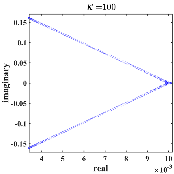
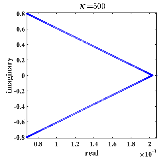
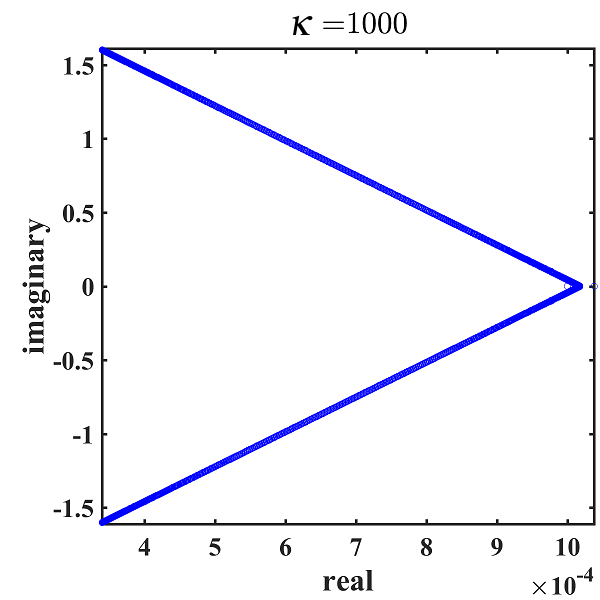
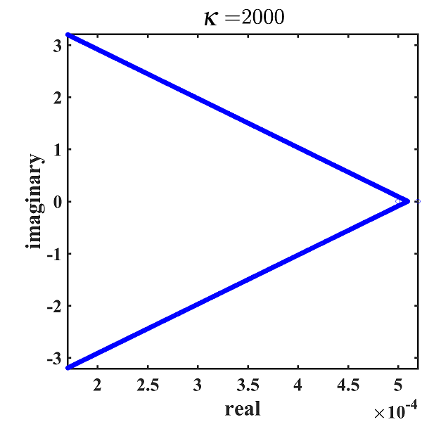
Figure 1: The spectral distribution of the linear system (57) for one dimensional dynamic equation with different subdivision $\kappa$ when $\epsilon=0.1$, $\Delta t=0.01$, $\sigma=100$, $n=1$ and $k=1$.

Table 1: The condition number of the linear system (57) for one dimensional dynamic equation with different subdivision $\kappa$ when $\epsilon=0.1$, $\Delta t=0.01$, $\sigma=100$, $n=1$ and $k=1$.

$\kappa$	100	500	1000	2000
$\mbox{cond}(\mathcal{A})$	0.407e+03	1.009e+04	4.037e+04	1.624e+05

4.1 Schur complement preconditioner

From the above discussion, it is necessary to find appropriate preconditioners for solving the discretized system (57). In P.J.2017 and L.2018 , two preconditioners have been proposed for Ohta-Kawasaki equation when using the backward Euler scheme. In this subsection, we will present Schur complement preconditioners for CSS similar to the construction technique in L.2018 . Moreover, we will analyze the spectral distribution of the preconditioning system.

Denote $\zeta=\Delta t/(1+\sigma\Delta t).$ Using Schur complement method and ignoring the influence of $L^{(n,k)}$, the Schur block preconditioner (Schur in short) for (57) is

$$\mathcal{P}_{Schur}=\left(\begin{array}[]{cc}M&\zeta S\\ -\epsilon^{2}S&M+2\epsilon\sqrt{\zeta}S\end{array}\right).$$

The spectral distribution for the preconditioning system is shown as follows.

Theorem 4.1

The eigenvalues of $\mathcal{P}_{Schur}^{-1}\hat{\mathcal{A}}$ are real and satisfy

$$\lambda(\mathcal{P}_{Schur}^{-1}\hat{\mathcal{A}})\in(\frac{1}{2},1+\frac{1}{4\epsilon}\sqrt{\zeta}\lambda_{+}),$$

with $\lambda_{+}=\lambda_{\mbox{max}}(M^{-1}L^{(n,k)})$ and

$$\hat{\mathcal{A}}=\left(\begin{array}[]{cc}M&\zeta S\\ -\epsilon^{2}S-L^{(n,k)}&M\\ \end{array}\right).$$

Proof

Notice that

$$\tilde{K}=(M+\epsilon\sqrt{\zeta}S)M^{-1}(M+\epsilon\sqrt{\zeta}S)$$

is a good approximation of the Schur complement:

$$K=M+\epsilon^{2}\zeta SM^{-1}S+\zeta L^{(n,k)}M^{-1}S.$$

It is obvious that

$$\mathcal{P}_{Schur}^{-1}\mathcal{A}=\begin{pmatrix}I&M^{-1}B_{1}\\ 0&I\end{pmatrix}^{-1}\begin{pmatrix}I&0\\ \tilde{K}^{-1}L^{(n,k)}&\tilde{K}^{-1}K\end{pmatrix}\begin{pmatrix}I&M^{-1}B_{1}\\ 0&I\end{pmatrix}.$$ (58)

Then, it is required to prove

$$\lambda(\tilde{K}^{-1}K)\in(\frac{1}{2},1+\frac{1}{4\epsilon}\sqrt{\zeta}\lambda_{+})$$

and the corresponding eigenvalues are real.

Suppose $v$ is the corresponding eigenvector of the eigenvalue $\lambda(\tilde{K}^{-1}K)$, thus

$$Kv=\lambda\tilde{K}v.$$ (59)

i) If $v\in\mbox{null}(S)$, by (59), then $Mv=\lambda Mv$, which implies that $\lambda=1$.

ii) If $v\notin\mbox{null}(S)$, using (59), we have

$$SM^{-1}Kv=\lambda SM^{-1}\tilde{K}v.$$

It follows that

$$v^{*}Fv=\lambda v^{*}Gv,$$ (60)

where

$$F=SM^{-1}K=S+\epsilon^{2}\zeta SM^{-1}SM^{-1}S+\zeta SM^{-1}L^{(n,k)}M^{-1}S,$$

$$G=SM^{-1}\tilde{K}=S+\epsilon^{2}\zeta SM^{-1}SM^{-1}S+2\epsilon\sqrt{\zeta}SM^{-1}S.$$

As $F$ and $G$ are real symmetric, then $v^{*}Fv$ and $v^{*}Gv$ are real (with $v^{*}Gv$ also positive). The eigenvalues of $\lambda(\tilde{K}^{-1}K)$ are real. Using (60), we get

$$\lambda=\frac{v^{*}Fv}{v^{*}Gv} =\frac{v^{*}Sv+\epsilon^{2}\zeta v^{*}SM^{-1}SM^{-1}Sv+\zeta v^{*}SM^{-1}L^{(n,k)}M^{-1}Sv}{v^{*}Sv+\epsilon^{2}\zeta v^{*}SM^{-1}SM^{-1}Sv+2\epsilon\sqrt{\zeta}v^{*}SM^{-1}Sv}$$

$$=1-\frac{2\epsilon\sqrt{\zeta}v^{*}SM^{-1}Sv}{v^{*}Sv+2\epsilon\sqrt{\zeta}v^{*}SM^{-1}Sv+\epsilon^{2}\zeta v^{*}SM^{-1}SM^{-1}Sv}$$

$$~{}~{}~{}~{}+\frac{\zeta v^{*}SM^{-1}L^{(n,k)}M^{-1}Sv}{v^{*}Sv+2\epsilon\sqrt{\zeta}v^{*}SM^{-1}Sv+\epsilon^{2}\zeta v^{*}SM^{-1}SM^{-1}Sv}$$

$$=1-\mathcal{R}_{1}+\mathcal{R}_{2}.$$ (61)

It is evident that $\mathcal{R}_{1}>0$. Writing

$$a=S^{\frac{1}{2}}v,~{}b=\epsilon\sqrt{\zeta}S^{\frac{1}{2}}M^{-1}Sv,$$

combining with the inequality $a^{*}a+b^{*}b\geq a^{*}b+b^{*}a$, it follows that

$$\mathcal{R}_{1}=(a^{*}b+b^{*}a)/(a^{*}a+b^{*}b+a^{*}b+b^{*}a)\leq\frac{1}{2}.$$

Therefore, we have

$$\mathcal{R}_{1}\in(0,\frac{1}{2}].$$ (62)

Noting

$$\mathcal{R}_{2} =\zeta\frac{v^{*}SM^{-1}L^{(n,k)}M^{-1}Sv}{v^{*}SM^{-1}Sv}\cdotp\frac{v^{*}SM^{-1}Sv}{v^{*}Sv+2\epsilon\sqrt{\zeta}v^{*}SM^{-1}Sv+\epsilon^{2}\zeta v^{*}SM^{-1}SM^{-1}Sv}$$

$$=\zeta\mathcal{R}_{21}\cdotp\mathcal{R}_{22},$$

then

$$\mathcal{R}_{22}=\frac{1}{2\epsilon\sqrt{\zeta}}\mathcal{R}_{1},$$

which shows that

$$\mathcal{R}_{22}\in(0,\frac{1}{4\epsilon\sqrt{\zeta}}].$$

Writing

$$\bar{v}=M^{-\frac{1}{2}}Sv,$$

we immediately have

$$\mathcal{R}_{21}=\frac{\bar{v}^{*}M^{-\frac{1}{2}}L^{(n,k)}M^{-\frac{1}{2}}\bar{v}}{\bar{v}^{*}\bar{v}}\in[\lambda_{\mbox{min}}(M^{-1}L^{(n,k)}),\lambda_{\mbox{max}}(M^{-1}L^{(n,k)})],$$

where $\lambda_{\mbox{min}}(M^{-1}L^{(n,k)})>0$. Combining with the derived bounds, it is obvious that

$$\mathcal{R}_{2}\in(0,\frac{1}{4\epsilon}\sqrt{\zeta}\lambda_{+}].$$ (63)

Substituting (62) and (63) into (61), it follows that

$$\lambda(\tilde{K}^{-1}K)\in(\frac{1}{2},1+\frac{1}{4\epsilon}\sqrt{\zeta}\lambda_{+}).$$

Combining this with (58), we complete the proof.

4.2 MHSS preconditioner

In this section, using the structure of the linear system (57), we propose a block preconditioner based on the MHSS and analyze the eigenvalue distribution of the preconditioning system.

The linear system (57) can be rearranged equivalently to the two-by-two block system:

$$\tilde{\mathcal{A}}\left(\begin{array}[]{c}U^{(n,k)}\\ W^{(n,k)}\\ \end{array}\right)=\left(\begin{array}[]{cc}\epsilon^{2}S+L^{(n,k)}&-M\\ M&\zeta S\\ \end{array}\right)\left(\begin{array}[]{c}U^{(n,k)}\\ W^{(n,k)}\\ \end{array}\right)=\left(\begin{array}[]{c}-E^{(n,k)}\\ \frac{1}{1+\sigma\Delta t}F^{(n)}\end{array}\right)=b.$$ (72)

Let $A=\epsilon^{2}S+L^{(n,k)},~{}~{}B=\zeta S,$ then

$$\tilde{\mathcal{A}}=\left(\begin{array}[]{cc}A&-M\\ M&B\\ \end{array}\right).$$

Denote $\tilde{p}=\kappa-1$, thus $A\in\mathbb{R}^{\tilde{p}\times\tilde{p}}$ and $A\succ 0$, $B\in\mathbb{R}^{\tilde{p}\times\tilde{p}}$ and $B\succeq 0$. The rearranged linear system (72) is a generalized saddle point problem, which widely exists in scientific computing and numerical algebra.

In recent years, many works have been devoted to developing efficient preconditioners for the generalized saddle point problem, such as block diagonal and triangular preconditioners (O.2015 -Y.C.J.2010 ), matrix splitting preconditioners (G.Z.2016 -L.L.G.2019 ). Among the preconditioners, the HSS preconditioner is an efficient method to solve the generalized saddle point problem, originally developed by Bai et al. G.B.2003 . However, directly applying the HSS method to (72) will result in inefficiency. As an improvement, we present an MHSS block preconditioner for the linear system (72).

Using the similar constructing technique as L.L.G.2019 , for any constant $\alpha>0$, the MHSS block preconditioner $\mathcal{P}_{MHSS}$ is defined by:

$$\mathcal{P}_{MHSS}=\left(\begin{array}[]{cc}\frac{1}{\alpha}A&0\\ 0&I\\ \end{array}\right)\left(\begin{array}[]{cc}\alpha I&-M\\ M&B\end{array}\right).$$ (77)

Let

$$\mathcal{R}=\mathcal{P}_{MHSS}-\tilde{\mathcal{A}}=\left(\begin{array}[]{cc}0&M-\frac{1}{\alpha}AM\\ 0&0\\ \end{array}\right),$$

then

$$\tilde{\mathcal{A}}=\mathcal{P}_{MHSS}-\mathcal{R}.$$

Decomposing $\mathcal{P}_{MHSS}$ as

$$\begin{split}\mathcal{P}_{MHSS}=\frac{1}{\alpha}\left(\begin{array}[]{cc}A&0\\ 0&\alpha I\\ \end{array}\right)\left(\begin{array}[]{cc}I&0\\ \frac{1}{\alpha}M&I\\ \end{array}\right)\left(\begin{array}[]{cc}\alpha I&0\\ 0&B+\frac{1}{\alpha}M^{2}\\ \end{array}\right)\left(\begin{array}[]{cc}I&-\frac{1}{\alpha}M\\ 0&I\\ \end{array}\right),\end{split}$$

then we obtain

$$\begin{split}\mathcal{T}(\alpha)&=\mathcal{P}_{MHSS}^{-1}\mathcal{R}\\ &=\left(\begin{array}[]{cc}0&A^{-1}M-\frac{1}{\alpha}M+\frac{1}{\alpha}M(B+\frac{1}{\alpha}M^{2})^{-1}(\frac{1}{\alpha}M^{2}-MA^{-1}M)\\ 0&(B+\frac{1}{\alpha}M^{2})^{-1}(\frac{1}{\alpha}M^{2}-MA^{-1}M)\\ \end{array}\right).\end{split}$$ (78)

Writing

$$D=B+\frac{1}{\alpha}M^{2},~{}~{}F=\frac{1}{\alpha}M^{2}-MA^{-1}M,$$ (79)

thus (78) turns to

$$\mathcal{T}(\alpha)=\left(\begin{array}[]{cc}0&A^{-1}M-\frac{1}{\alpha}M+\frac{1}{\alpha}MD^{-1}F\\ 0&D^{-1}F\\ \end{array}\right).$$ (82)

Therefore, we obtain the preconditioned system

$$\begin{split}\mathcal{P}_{MHSS}^{-1}\tilde{\mathcal{A}}=\mathcal{P}_{MHSS}^{-1}(\mathcal{P}_{MHSS}-\mathcal{R})&=I-\mathcal{P}_{MHSS}^{-1}\mathcal{R}\\ &=I-\mathcal{T}(\alpha)\\ &=\left(\begin{array}[]{cc}I&-A^{-1}M+\frac{1}{\alpha}M-\frac{1}{\alpha}MD^{-1}F\\ 0&I-D^{-1}F\\ \end{array}\right),\end{split}$$ (83)

where $D$ and $F$ are defined by (79).

Now, we analyze the spectral distribution for the preconditioned matrix $\mathcal{P}_{MHSS}^{-1}\tilde{\mathcal{A}}$.

Theorem 4.2

Let $A\in\mathbb{R}^{\tilde{p}\times\tilde{p}}$, $M\in\mathbb{R}^{\tilde{p}\times\tilde{p}}$ and $M\succ 0$, $B\in\mathbb{R}^{\tilde{p}\times\tilde{p}}$ and $B\succeq 0$, $\alpha$ be a positive constant. Then the preconditioned matrix $\mathcal{P}_{MHSS}^{-1}\tilde{\mathcal{A}}$ has at least $\tilde{p}$ eigenvalues $1$. The remaining eigenvalues $\lambda$ are real and located in the positive interval

$$\frac{\alpha c_{\tilde{p}}^{2}}{\theta_{1}(c_{1}^{2}+\alpha\sigma_{1})}\leq\lambda\leq\frac{\alpha(\sigma_{1}\theta_{\tilde{p}}+c_{1}^{2})}{\theta_{\tilde{p}}c_{\tilde{p}}^{2}},$$ (84)

where $\sigma_{\tilde{p}}$, $c_{\tilde{p}}$, $\theta_{\tilde{p}}$ and $\sigma_{1}$, $c_{1}$, $\theta_{1}$ are the minimum and maximum eigenvalues of $B,~{}M,~{}A$, respectively. Furthermore, if $A=\alpha I$, then all the eigenvalues of $\mathcal{P}_{MHSS}^{-1}\tilde{\mathcal{A}}$ are $1$.

Proof

From (83), it is evident that $\mathcal{P}_{MHSS}^{-1}\tilde{\mathcal{A}}$ has at least $\tilde{p}$ eigenvalues $1$. The remaining are the eigenvalues of $I-D^{-1}F$. Let

$$I-D^{-1}F=D^{-1}(D-F)=(B+\frac{1}{\alpha}M^{2})^{-1}(B+MA^{-1}M),$$

$\lambda$ and $u$ be the eigenvalue and corresponding eigenvector of $I-D^{-1}F$, thus

$$(B+MA^{-1}M)u=\lambda~{}(B+\frac{1}{\alpha}M^{2})u.$$ (85)

Premultiplying both sides of (85) by $u^{\ast}/(u^{\ast}u)$ gets

$$\frac{u^{\ast}(B+MA^{-1}M)u}{u^{\ast}u}=\lambda\frac{u^{\ast}(B+\frac{1}{\alpha}M^{2})u}{u^{\ast}u}.$$

Define

$$d=\frac{u^{\ast}MA^{-1}Mu}{u^{\ast}u},~{}\gamma=\frac{u^{\ast}Bu}{u^{\ast}u},~{}\mbox{and}~{}\tau=\frac{u^{\ast}M^{2}u}{u^{\ast}u},$$ (86)

then

$$\lambda=\frac{{\alpha}(\gamma+d)}{{\alpha}\gamma+\tau}.$$ (87)

Note that $A\succ 0,~{}M\succ 0$ and $B\succeq 0$. Using (86), then

$$0<\frac{c_{\tilde{p}}^{2}}{\theta_{1}}\leq d\leq\frac{c_{1}^{2}}{\theta_{n}},~{}0<c_{\tilde{p}}^{2}\leq\tau\leq c_{1}^{2},~{}\mbox{and}~{}0\leq\gamma\leq\sigma_{1}.$$ (88)

Combining (87) with (88), we obtain (84).

Remark 2

Noting that the positive interval presented in Theorem 4.2 is not very tight. Therefore, choosing appropriate $\lambda$ could obtain a better spectral distribution. This is illustrated by a simple numerical experiment in Figure 2.

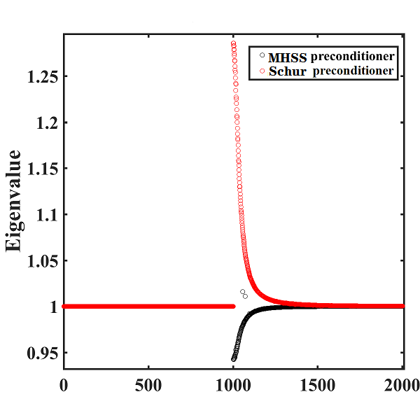
Figure 2: The spectral distribution of the preconditioned linear system with $\hat{M}=1000,~{}\epsilon=0.01,~{}dt=0.001,~{}\sigma=10,~{}n=1,~{}k=1$, $\alpha=0.001$.

In the following, we present an approach to get $\alpha$ such that $\rho(\mathcal{T}(\alpha))$ as small as possible. However, it is difficult to compute $\rho(\mathcal{T}(\alpha))$ exactly. Instead, we give an upper bound of $\rho(\mathcal{T}(\alpha))$.

Theorem 4.3

Let $A\succ 0,~{}M\succ 0\in\mathbb{R}^{\tilde{p}\times\tilde{p}}$ and, $B\succeq 0\in\mathbb{R}^{\tilde{p}\times\tilde{p}}$. Assume that $\mathcal{T}(\alpha)$ is defined in (82). Then, we get

$$\rho(\mathcal{T}(\alpha))\leq\max_{1\leq i\leq\tilde{p}}\Big{|}1-\frac{\alpha}{\lambda_{i}(A)}\Big{|}=\tilde{\sigma}(\alpha).$$

Proof

By the definition of $\mathcal{T}(\alpha)$ in (82), it follows that

$$\rho(\mathcal{T}(\alpha))=\rho(D^{-1}F),$$

where $D$ and $F$ are defined in (79). Note that

$$D^{-1}F=M^{-1}\tilde{D}^{-1}\tilde{F}M,$$

where

$$\tilde{D}=\frac{1}{\alpha}I+M^{-1}BM^{-1},~{}~{}\tilde{F}=\frac{1}{\alpha}I-A^{-1}.$$

Thus

$$\rho(\mathcal{T}(\alpha))=\rho(D^{-1}F)=\rho(\tilde{D}^{-1}\tilde{F})\leq\|\tilde{D}^{-1}\tilde{F}\|_{2}\leq\|\tilde{D}^{-1}\|_{2}\|\tilde{F}\|_{2}.$$

Since $A>0$, $M>0$ and $B\geq 0$, we have

$$\|\tilde{D}^{-1}\|_{2}=\Big{\|}(\frac{1}{\alpha}I+M^{-1}BM^{-1})^{-1}\Big{\|}_{2} =\max_{1\leq i\leq\tilde{p}}\Big{|}\lambda_{i}[(\frac{1}{\alpha}I+M^{-1}BM^{-1})^{-1}]\Big{|}$$

$$=\max_{1\leq i\leq\tilde{p}}\left|\frac{1}{\frac{1}{\alpha}+\lambda_{i}(M^{-1}BM^{-1})}\right|=\alpha,$$

and

$$\|\tilde{F}\|_{2}=\Big{\|}\frac{1}{\alpha}I-A^{-1}\Big{\|}_{2} =\max_{1\leq i\leq\tilde{p}}\Big{|}\lambda_{i}(\frac{1}{\alpha}I-A^{-1})\Big{|}$$

$$=\max_{1\leq i\leq\tilde{p}}\Big{|}\frac{1}{\alpha}-\lambda_{i}(A^{-1})\Big{|}.$$

Hence,

$$\rho(\mathcal{T}(\alpha))=\rho(D^{-1}F)\leq\alpha\max_{1\leq i\leq\tilde{p}}\Big{|}\frac{1}{\alpha}-\lambda_{i}(A^{-1})\Big{|}=\max_{1\leq i\leq\tilde{p}}\Big{|}1-\frac{\alpha}{\lambda_{i}(A)}\Big{|}.$$

Remark 3

By Theorem 4.3, we can choose $\alpha$ as the optimal $\alpha_{*}$ to minimize $\tilde{\sigma}(\alpha)$. Therefore,

$$\alpha=\alpha_{*}=\mbox{arg}~{}\min_{\alpha}\tilde{\sigma}(\alpha)=\frac{2\lambda_{1}(A)\lambda_{\tilde{p}}(A)}{\lambda_{1}(A)+\lambda_{\tilde{p}}(A)}.$$

Since $\alpha_{*}$ is related to the eigenvalues of $A$, it is expensive to compute the optimal parameter $\alpha_{*}$ for large scale matrix $A$. Therefore, in practical implementation, we need to make an approximation for $\alpha_{*}$, refer to H.2014 . The practical choice strategy for parameter $\alpha$ is

$$\alpha=\frac{\mbox{trace}(A)}{\tilde{p}}~{}~{}\mbox{or}~{}~{}\alpha=\frac{\mbox{trace}(M^{4})}{\mbox{trace}(M^{4}A^{-1})}.$$

5 Numerical results

In this section, we offer several examples to support the theoretical analysis. The spatial domain $\mathcal{T}_{h}$ is uniformly discreted for $t_{n}=n\Delta t$ $(0\leq n\leq N)$. The piecewise linear functions are used as the basis functions. GMRES is adopted to solve the preconditioned linear system (57) in each iteration. The elapsed CPU time per nonlinear iteration process in seconds is denoted by ‘CPU’ and the average of GMRES iteration per Newton step by IT_GM. Let $k_{n}$ be the iteration steps of the $n$-th nonlinear iteration, and IT_tol be the total iteration steps after $n$-th nonlinear iteration, i.e., $\mbox{IT}_{tol}=\sum_{i=1}^{n}k_{i}$. The nonlinear iteration error is defined as $\varepsilon=||u^{(n,k)}-u^{(n,k-1)}||_{2}$. The stop criteria $\varepsilon$ is chosen as $10^{-6}$.

First, we demonstrate the performance of two Newton iteration methods. When the total number of time steps is $N=100$, Tab. 2 compares two Newton methods against CPU and $\mbox{IT}_{tol}$ in one and two dimensional space with different degree of freedom (DOF). Obviously, the Newton method requires less CPU and $\mbox{IT}_{tol}$ than those of the V-N method.

Table 2: A comparison of two Netwon methods with different DOF for domains $\Omega=[0,1]$ and $\Omega=[0,\pi]^{2}$.

$\{\Omega,~{}~{}\epsilon\}$		$\{[0,1],~{}~{}0.01\}$			$\{[0,\pi]^{2},~{}~{}0.001\}$
DOF	Index	Newton	V-N	DOF	Index	Newton	V-N
$10^{4}$	CPU(s)	15.56	57.12	$10^{4}$	CPU	52.54	84.76
	ITtol	346	1359		ITtol	300	486
$4\times 10^{5}$	CPU	683.30	2371.97	$4\times 10^{4}$	CPU	301.78	750.69
	ITtol	327	1183		ITtol	300	753

Furthermore, Fig. 3 gives the concrete iteration process when $\Omega=[0,1]$, DOF$=10^{4}$, $\sigma=100$, $\Delta t=\epsilon^{2}$ and $\epsilon=0.01$. Note that the CPU time required for each nonlinear iteration step of two Newton methods is almost the same. Fig. 3(a) represents that the Newton method requires fewer nonlinear iteration steps than that of the V-N method for each time step $n$, as well as CPU time. When $n=23$, Fig. 3(b) illustrates that the error $\varepsilon$ of the Newton method decreases faster than that of the V-N method, as the theory in Sec. 3 predicted. Similar phenomena also appear for other cases in Tab. 2.

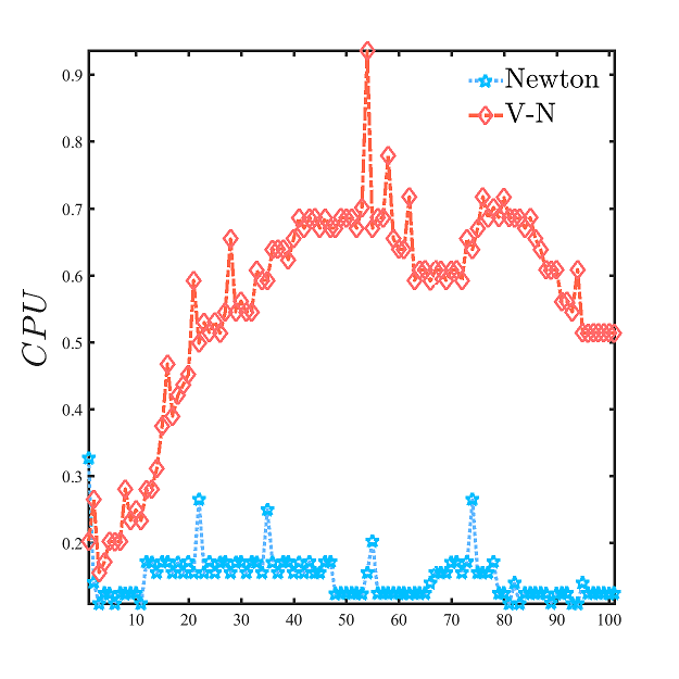
(a) CPU time against iterations

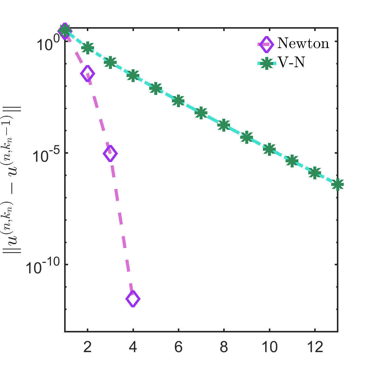
(b) Error tendency of the $23^{th}$ nonlinear iteration

Figure 3: Comparison of convergence speed between the Newton method and the V-N method with $\Omega=[0,1]$ and DOF$=10^{4}$.

Second, we demonstrate the efficiency of proposed preconditioners when solving linear system (57). As an one-dimensional example, Table 3 presents the performance of solving non-preconditioned and preconditioned systems in $500$ time steps ($\Delta t=\epsilon^{2}$) with different spatial DOF for domains $\Omega=[0,1]$. From these results, it can be seen that two preconditioners accelerate computation, almost three times faster than solving non-preconditioned system in terms of CPU time.

Table 3: A comparison of computing non-preconditioned and preconditioned systems in $500$ time steps ($\Delta t=\epsilon^{2}$) with different spatial DOF and $\Omega=[0,1]$.

$DOF$	Index	($\epsilon$,$\sigma$)	TGM	ITtol	CPU (s)
	Newton		-		263.15
	Newton-$\mathcal{P}_{Schur}$	(0.001,100)	5.5	1500	101.97
	Newton-$\mathcal{P}_{MHSS}$		14.5		107.96
$10^{4}$	V-N		-		422.81
	V-N-$\mathcal{P}_{Schur}$	(0.001,100)	5.0	2349	156.65
	V-N-$\mathcal{P}_{MHSS}$		7.5		165.27
	Newton		-		1539.59
	Newton-$\mathcal{P}_{Schur}$	(0.001,100)	7.0	1500	592.27
	Newton-$\mathcal{P}_{MHSS}$		8.4		580.30
$4\times 10^{4}$	V-N		-		3553.33
	V-N-$\mathcal{P}_{Schur}$	(0.001,100)	6.5	3291	1271.09
	V-N-$\mathcal{P}_{MHSS}$		16.9		1267.39

Last, we observe the long-time behavior of the proposed method in the domain $\Omega=[0,\pi]^{2}$ with $1000\times 1000$ triangular grids. Using random initial values, Figs. 4 and 5 show the coarsening dynamic process with different parameters. The final converged morphologies are lamellar and cylindrical phases, respectively. As shown in these figures, our method keeps energy dissipation as time evolves.

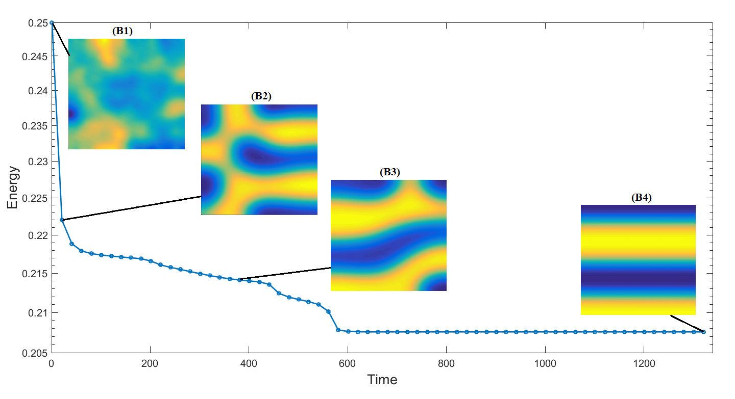
Figure 4: The dynamic process in domain $[0,\pi]^{2}$ when $\epsilon=0.08$, $\sigma=10$ , $m=0$ and $\Delta t=0.01$ with a random initial value. (B1), (B2), (B3) and (B4) correspond to $t=0,0.2,4,13.43$.

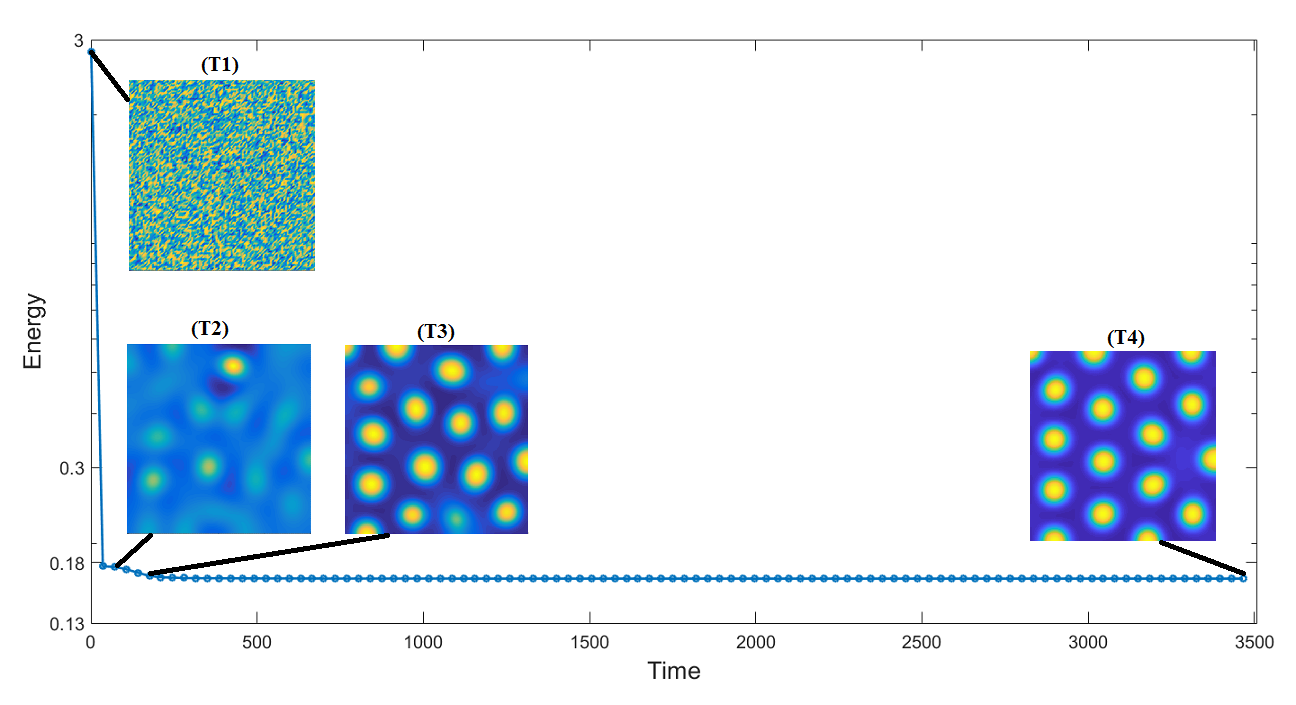
Figure 5: The dynamic process in domain $[0,\pi]^{2}$ when $\epsilon=0.08$, $\sigma=10$ , $m=0.4$ and $\Delta t=0.0064$ with a random initial value. (T1), (T2), (T3) and (T4) correspond to $t=0,0.448,1.344,22.4$.

6 Conclusion

This paper presents a systematic numerical method to solve the mass-conserved Ohta-Kawasaki equation. An unconditionally energy stable scheme, the CSS, is used to discretize the time variable, while the FEM to the spatial variable. Two Newton methods are applied to update the implicit nonlinear terms. To reduce the condition number of the discretized linear system, we propose Schur complement preconditioner and MHSS block preconditioner. The convergent rate of the two Newton iteration method has been proven to be the same, while the Newton method has a smaller convergent factor than the variant one. The spectral distribution of two block preconditioning linear systems has been analyzed. Numerical investigations provided sufficient support for the theoretical analysis and demonstrated the efficiency of the proposed numerical methods.

Appendix A.  Proof of Theorem 2.1.

Proof

Using the definition of $E(u)$ in (1), then

$$E(u^{n})-E(u^{n-1}) =\frac{1}{2}\epsilon^{2}(\|\nabla u^{n}\|^{2}-\|\nabla u^{n-1}\|^{2})+(\Phi(u^{n})-\Phi(u^{n-1}),1)$$

$$~{}~{}+\frac{1}{2}\sigma(\|(-\Delta)^{-\frac{1}{2}}(u^{n}-m)\|^{2}-\|(-\Delta)^{-\frac{1}{2}}(u^{n-1}-m)\|^{2}).$$ (89)

Using Taylor expansion, we have

$$\Phi_{+}(u^{n-1})-\Phi_{+}(u^{n})=\Phi^{\prime}_{+}(u^{n})(u^{n-1}-u^{n})+\frac{\Phi_{+}^{{}^{\prime\prime}}(\xi^{n-1})}{2}(u^{n-1}-u^{n})^{2},$$

$$\Phi_{-}(u^{n})-\Phi_{-}(u^{n-1})=\Phi^{\prime}_{-}(u^{n-1})(u^{n}-u^{n-1})+\frac{\Phi_{-}^{{}^{\prime\prime}}(\eta^{n-1})}{2}(u^{n}-u^{n-1})^{2}.$$

Thus,

$$\Phi(u^{n})-\Phi(u^{n-1}) =-(\Phi_{+}(u^{n-1})-\Phi_{+}(u^{n}))-(\Phi_{-}(u^{n})-\Phi_{-}(u^{n-1}))$$

$$=(\Phi^{\prime}_{+}(u^{n})-\Phi^{\prime}_{-}(u^{n-1}))(u^{n}-u^{n-1})-\frac{1}{2}(\Phi_{+}^{{}^{\prime\prime}}(\xi^{n-1})+\Phi_{-}^{{}^{\prime\prime}}(\eta^{n-1}))(u^{n}-u^{n-1})^{2}.$$ (90)

Combing the identity

$$a^{2}-b^{2}=2a(a-b)-(a-b)^{2}$$

with (90), (89) is equivalent to

$$E(u^{n})-E(u^{n-1})$$

$$=\epsilon^{2}(\nabla u^{n},\nabla(u^{n}-u^{n-1}))-\frac{1}{2}\epsilon^{2}\|\nabla(u^{n}-u^{n-1})\|^{2}$$

$$~{}~{}+(\Phi^{\prime}_{+}(u^{n})-\Phi^{\prime}_{-}(u^{n-1}),u^{n}-u^{n-1})-\frac{1}{2}(\Phi_{+}^{{}^{\prime\prime}}(\xi^{n-1})+\Phi_{-}^{{}^{\prime\prime}}(\eta^{n-1}),(u^{n}-u^{n-1})^{2})$$

$$~{}~{}+\sigma((-\Delta)^{-\frac{1}{2}}(u^{n}-m),(-\Delta)^{-\frac{1}{2}}(u^{n}-u^{n-1}))-\frac{1}{2}\sigma\|(-\Delta)^{-\frac{1}{2}}(u^{n}-u^{n-1})\|^{2}$$

$$=(-\epsilon^{2}\Delta u^{n},u^{n}-u^{n-1})-\frac{1}{2}\epsilon^{2}\|\nabla(u^{n}-u^{n-1})\|^{2}$$

$$~{}~{}+(\Phi^{\prime}_{+}(u^{n})-\Phi^{\prime}_{-}(u^{n-1}),u^{n}-u^{n-1})-\frac{1}{2}(\Phi_{+}^{{}^{\prime\prime}}(\xi^{n-1})+\Phi_{-}^{{}^{\prime\prime}}(\eta^{n-1}),(u^{n}-u^{n-1})^{2})$$

$$~{}~{}+\sigma((-\Delta)^{-1}(u^{n}-m),u^{n}-u^{n-1})-\frac{1}{2}\sigma\|(-\Delta)^{-\frac{1}{2}}(u^{n}-u^{n-1})\|^{2}$$

$$=(-\epsilon^{2}\Delta u^{n}+\Phi^{\prime}_{+}(u^{n})-\Phi^{\prime}_{-}(u^{n-1})+\sigma(-\Delta)^{-1}(u^{n}-m),u^{n}-u^{n-1})$$

$$~{}~{}-\frac{1}{2}\epsilon^{2}\|\nabla(u^{n}-u^{n-1})\|^{2}-\frac{1}{2}(\Phi_{+}^{{}^{\prime\prime}}(\xi^{n-1})+\Phi_{-}^{{}^{\prime\prime}}(\eta^{n-1}),(u^{n}-u^{n-1})^{2})$$

$$~{}~{}-\frac{1}{2}\sigma\|(-\Delta)^{-\frac{1}{2}}(u^{n}-u^{n-1})\|^{2}.$$ (91)

Taking the test function $v=u^{n}-u^{n-1}$ in (9), then

$$(\frac{u^{n}-u^{n-1}}{\Delta t},u^{n}-u^{n-1})+(\nabla w^{n},\nabla(u^{n}-u^{n-1}))+\sigma(u^{n}-m,u^{n}-u^{n-1})=0,$$ (92a)

$$(w^{n},u^{n}-u^{n-1})-\epsilon^{2}(\nabla u^{n},\nabla(u^{n}-u^{n-1}))-(\Phi^{\prime}_{+}(u^{n})-\Phi^{\prime}_{-}(u^{n-1}),u^{n}-u^{n-1})=0.$$ (92b)

Putting

$$\mu^{n}=w^{n}+\sigma(-\Delta)^{-1}(u^{n}-m)$$

into (92a), rearranging (92b), thus

$$(\frac{u^{n}-u^{n-1}}{\Delta t},u^{n}-u^{n-1})=(\Delta\mu^{n},u^{n}-u^{n-1}),$$ (93a)

$$(w^{n},u^{n}-u^{n-1})=-\epsilon^{2}(\Delta u^{n},u^{n}-u^{n-1})+(\Phi^{\prime}_{+}(u^{n})-\Phi^{\prime}_{-}(u^{n-1}),u^{n}-u^{n-1}).$$ (93b)

Note that

$$\Phi_{+}(u)\geq 0,~{}~{}\Phi_{-}(u)\geq 0.$$

Substituting(93a) and (93b) into (91) yields

$$E(u^{n})-E(u^{n-1})$$

$$=(\mu^{n},u^{n}-u^{n-1})-\frac{1}{2}\epsilon^{2}\|\nabla(u^{n}-u^{n-1})\|^{2}$$

$$~{}~{}-\frac{1}{2}(\Phi_{+}^{{}^{\prime\prime}}(\xi^{n-1})+\Phi_{-}^{{}^{\prime\prime}}(\eta^{n-1}),(u^{n}-u^{n-1})^{2})-\frac{1}{2}\sigma\|(-\Delta)^{-\frac{1}{2}}(u^{n}-u^{n-1})\|^{2}.$$

By the definition of $\mu^{n}$ and let the test function $v=\mu^{n}$ in (9), we can obtain

$$(\mu^{n},u^{n}-u^{n-1})=\Delta t(\mu^{n},\Delta\mu^{n}),$$

then

$$E(u^{n})-E(u^{n-1})$$

$$=\Delta t(\mu^{n},\Delta\mu^{n})-\frac{1}{2}\epsilon^{2}\|\nabla(u^{n}-u^{n-1})\|^{2}$$

$$~{}~{}-\frac{1}{2}(\Phi_{+}^{{}^{\prime\prime}}(\xi^{n-1})+\Phi_{-}^{{}^{\prime\prime}}(\eta^{n-1}),(u^{n}-u^{n-1})^{2})-\frac{1}{2}\sigma\|(-\Delta)^{-\frac{1}{2}}(u^{n}-u^{n-1})\|^{2}\leq 0,$$

which implies (10). Thus we complete the proof of Theorem 2.1.

Appendix B.  Proof of Theorem 2.2.

Lemma 4

E.2010 (Poincar$\acute{\mbox{e}}$ inequality) Let $\Omega$ be a bounded, connected, open subset of $\mathbb{R}^{d}$ with boundary $\partial\Omega$ of $\mathbb{C}^{1}$. Then there exists a constant $c$, depending only on $d$ and $\Omega$ such that

$$\left\|v-\int_{\Omega}v\,dx\right\|\leq c\|\nabla v\|.$$

Definition 1

P.Q.2012 For $u\in H^{1}(\Omega)$, we define $\Delta_{h}u\in V_{h}$ such that

$$(-\Delta_{h}u,v_{h})=(\nabla u,\nabla v_{h}),~{}~{}\forall v_{h}\in V_{h},$$

where the subscript ‘h’ means that $\Delta_{h}u$ depends on the discretization mesh.

Proof of Theorem 2.2.

Proof

From Poincar$\acute{\mbox{e}}$ inequality (Lemma 4), we have

$$\|u^{n}_{h}-m\|=\left\|u^{n}_{h}-\int_{\Omega}u^{n}_{h}\,dx\right\|\leq c\|\nabla u^{n}_{h}\|.$$

Then

$$\|u_{h}^{n}\|-m|\Omega|\leq\|u_{h}^{n}-m\|\leq c\|\nabla u^{n}_{h}\|.$$ (94)

Set $v_{h}=w_{h}^{n}$ in (11a), then

$$\Big{(}\frac{u^{n}_{h}-u^{n-1}_{h}}{\Delta t},w_{h}^{n}\Big{)}+(\nabla w^{n}_{h},\nabla w_{h}^{n})+\sigma(u^{n}_{h}-m,w_{h}^{n})=0.$$ (95)

Taking $v_{h}=(u^{n}_{h}-u^{n-1}_{h})/\Delta t$ in (11b) yields

$$(w^{n}_{h},\frac{u^{n}_{h}-u^{n-1}_{h}}{\Delta t})=\epsilon^{2}(\nabla u^{n}_{h},\nabla\frac{u^{n}_{h}-u^{n-1}_{h}}{\Delta t})+(\Phi^{\prime}_{+}(u^{n}_{h})-\Phi^{\prime}_{-}(u^{n-1}_{h}),\frac{u^{n}_{h}-u^{n-1}_{h}}{\Delta t}).$$ (96)

Subtracting (95) from (96), using the symmetry in the inner product, thus

$$\epsilon^{2}\Big{(}\nabla u^{n}_{h},\frac{\nabla u^{n}_{h}-\nabla u^{n-1}_{h}}{\Delta t}\Big{)}+\Big{(}\Phi^{\prime}_{+}(u^{n}_{h}) -\Phi^{\prime}_{-}(u^{n-1}_{h}),\frac{u^{n}_{h}-u^{n-1}_{h}}{\Delta t}\Big{)}$$

$$+\|\nabla w^{n}_{h}\|^{2}+\sigma(u^{n}_{h}-m,w_{h}^{n})=0.$$ (97)

Note that

$$\nabla u^{n}_{h}=\frac{\nabla u^{n}_{h}-\nabla u^{n-1}_{h}}{2}+\frac{\nabla u^{n}_{h}+\nabla u^{n-1}_{h}}{2}.$$

Then (97) is equivalent to

$$\frac{\epsilon^{2}}{2\Delta t} \Big{\{}(\nabla(u^{n}_{h}-u^{n-1}_{h}),\nabla(u^{n}_{h}-u^{n-1}_{h}))+(\nabla u^{n}_{h}+\nabla u^{n-1}_{h},\nabla u^{n}_{h}-\nabla u^{n-1}_{h})\Big{\}}$$

$$+\Big{(}\Phi^{\prime}_{+}(u^{n}_{h})-\Phi^{\prime}_{-}(u^{n-1}_{h}),\frac{u^{n}_{h}-u^{n-1}_{h}}{\Delta t}\Big{)}+\|\nabla w^{n}_{h}\|^{2}+\sigma(u^{n}_{h}-m,w_{h}^{n})=0.$$ (98)

The sequence $u_{h}^{n}$ keeps mass conservation in P.Q.2012 , i.e.,

$$(u_{h}^{n}-m,1)=0~{}~{}\mbox{for}~{}~{}n=0,1,\cdots,N.$$ (99)

Multiplying (99) by $\int_{\Omega}w_{h}^{n}\,dx\in\mathbb{R}$ gets

$$(u_{h}^{n}-m,\int_{\Omega}w_{h}^{n}\,dx)=0.$$

Hence,

$$(u_{h}^{n}-m,w_{h}^{n})=(u_{h}^{n}-m,w_{h}^{n}-\int_{\Omega}w_{h}^{n}\,dx).$$ (100)

Combining (98) with (100), we have

$$\frac{\epsilon^{2}}{2\Delta t}\Big{\{}\|\nabla(u^{n}_{h}-u^{n-1}_{h})\|^{2}+\|\nabla u^{n}_{h}\|^{2}-\|\nabla u^{n-1}_{h}\|^{2}\Big{\}}+\frac{1}{\Delta t}(\Phi^{\prime}_{+}(u^{n}_{h})-\Phi^{\prime}_{-}(u^{n-1}_{h}),u^{n}_{h}-u^{n-1}_{h})$$

$$~{}~{}~{}~{}~{}~{}~{}~{}+\|\nabla w^{n}_{h}\|^{2}+\sigma(u^{n}_{h}-m,w_{h}^{n}-\int_{\Omega}w_{h}^{n}\,dx)=0.$$ (101)

Using Taylor expansion for $\Phi(b)$ at $a$, then

$$\Phi^{\prime}(a)(a-b)=\Phi(a)-\Phi(b)+\frac{1}{2}\Phi^{\prime\prime}(\eta)(b-a)^{2},~{}~{}\eta\in(a,b).$$

Notice that

$$\Phi^{\prime}_{+}(u)=u^{3},~{}~{}\Phi^{\prime}_{-}(u)=u,~{}~{}\Phi^{\prime\prime}_{+}(u)=3u^{2}>-1,~{}~{}\Phi^{\prime\prime}_{-}(u)=1.$$

Hence,

$$(\Phi_{+}(u_{h}^{n}),1)-(\Phi_{+}(u_{h}^{n-1}),1)-\frac{1}{2}\|u_{h}^{n}-u_{h}^{n-1}\|^{2}<(\Phi^{\prime}_{+}(u_{h}^{n}),u_{h}^{n}-u_{h}^{n-1}),$$ (102a)

$$(\Phi_{-}(u_{h}^{n-1}),1)-(\Phi_{-}(u_{h}^{n}),1)+\frac{1}{2}\|u_{h}^{n}-u_{h}^{n-1}\|^{2}=(\Phi^{\prime}_{-}(u_{h}^{n-1}),u_{h}^{n-1}-u_{h}^{n}).$$ (102b)

Substituting (102a) and (102b) in (101), multiplying by $2\Delta t$, then

$$\epsilon^{2}\|\nabla u^{n}_{h}\|^{2}+\epsilon^{2}\|\nabla(u^{n}_{h}-u^{n-1}_{h})\|^{2}+2(\Phi_{+}(u^{n}_{h}),1)+2(\Phi_{-}(u^{n-1}_{h}),1)+2\Delta t\|\nabla w^{n}_{h}\|^{2}$$

$$<\epsilon^{2}\|\nabla u^{n-1}_{h}\|^{2}+2(\Phi_{+}(u^{n-1}_{h}),1)+2(\Phi_{-}(u^{n}_{h}),1)-2\Delta t\sigma(u^{n}_{h}-m,w_{h}^{n}-\int_{\Omega}w_{h}^{n}\,dx)$$

$$<\epsilon^{2}\|\nabla u^{n-1}_{h}\|^{2}+2(\Phi_{+}(u^{n-1}_{h}),1)+2(\Phi_{-}(u^{n}_{h}),1)+2\Delta t\sigma\|u^{n}_{h}-m\|\cdotp\|w_{h}^{n}-\int_{\Omega}w_{h}^{n}\,dx\|$$

$$<\epsilon^{2}\|\nabla u^{n-1}_{h}\|^{2}+2(\Phi_{+}(u^{n-1}_{h}),1)+2(\Phi_{-}(u^{n}_{h}),1)+2\Delta t\sigma c^{2}\|\nabla u^{n}_{h}\|\cdotp\|\nabla w^{n}_{h}\|.$$ (103)

Applying the inequality $2ab\leq a^{2}+b^{2}$ to the last term on the right-hand side of (103), subtracting $\Delta t\|\nabla w^{n}_{h}\|^{2}$ from both sides of (103), then

$$\epsilon^{2}\|\nabla u^{n}_{h}\|^{2}+\epsilon^{2}\|\nabla(u^{n}_{h}-u^{n-1}_{h})\|^{2}+2(\Phi_{+}(u^{n}_{h}),1)+2(\Phi_{-}(u^{n-1}_{h}),1)+\Delta t\|\nabla w^{n}_{h}\|^{2}$$

$$<\epsilon^{2}\|\nabla u^{n-1}_{h}\|^{2}+2(\Phi_{+}(u^{n-1}_{h}),1)+2(\Phi_{-}(u^{n}_{h}),1)+\sigma^{2}c^{4}\Delta t\|\nabla u^{n}_{h}\|^{2}.$$ (104)

Summing (104) over $n=1,2,\cdots,\tilde{k}$ ($\tilde{k}\leq N$) yields

$$\epsilon^{2}\sum_{n=1}^{\tilde{k}}\|\nabla u^{n}_{h}\|^{2}+\epsilon^{2}\sum_{n=1}^{\tilde{k}}\|\nabla(u^{n}_{h}-u^{n-1}_{h})\|^{2}+2\sum_{n=1}^{\tilde{k}}(\Phi_{+}(u^{n}_{h}),1)+2\sum_{n=1}^{\tilde{k}}(\Phi_{-}(u^{n-1}_{h}),1)+\Delta t\sum_{n=1}^{\tilde{k}}\|\nabla w^{n}_{h}\|^{2}$$

$$<\epsilon^{2}\sum_{n=1}^{\tilde{k}}\|\nabla u^{n-1}_{h}\|^{2}+2\sum_{n=1}^{\tilde{k}}(\Phi_{+}(u^{n-1}_{h}),1)+2\sum_{n=1}^{\tilde{k}}(\Phi_{-}(u^{n}_{h}),1)+\sigma^{2}c^{4}\Delta t\sum_{n=1}^{\tilde{k}}\|\nabla u^{n}_{h}\|^{2}.$$ (105)

Canceling the same terms on each side of (105), then

$$\epsilon^{2}\|\nabla u^{\tilde{k}}_{h}\|^{2}+\epsilon^{2}\sum_{n=1}^{\tilde{k}}\|\nabla(u^{n}_{h}-u^{n-1}_{h})\|^{2}+2(\Phi_{+}(u^{\tilde{k}}_{h})-\Phi_{-}(u^{\tilde{k}}_{h}),1)+\Delta t\sum_{n=1}^{\tilde{k}}\|\nabla w^{n}_{h}\|^{2}$$

$$<\epsilon^{2}\|\nabla u^{0}_{h}\|^{2}+2(\Phi_{+}(u^{0}_{h})-\Phi_{-}(u^{0}_{h}),1)+\sigma^{2}c^{4}\Delta t\sum_{n=1}^{\tilde{k}}\|\nabla u^{n}_{h}\|^{2}.$$ (106)

For $\tilde{k}=1,2,\cdots,N$, note that

$$\Phi(u^{\tilde{k}}_{h})=\Phi_{+}(u_{h}^{\tilde{k}})-\Phi_{-}(u_{h}^{\tilde{k}})\geq 0.$$

Hence, (106) reduces to

$$\epsilon^{2}\|\nabla u^{\tilde{k}}_{h}\|^{2}<\epsilon^{2}\|\nabla u^{0}_{h}\|^{2}+2(\Phi_{+}(u^{0}_{h})-\Phi_{-}(u^{0}_{h}),1)+\sigma^{2}c^{4}\Delta t\sum_{n=1}^{\tilde{k}}\|\nabla u^{n}_{h}\|^{2}.$$

Thus,

$$(\epsilon^{2}-\sigma^{2}c^{4}\Delta t)\|\nabla u^{\tilde{k}}_{h}\|^{2}<\epsilon^{2}\|\nabla u^{0}_{h}\|^{2}+2(\Phi_{+}(u^{0}_{h})-\Phi_{-}(u^{0}_{h}),1)+\sigma^{2}c^{4}\Delta t\sum_{n=1}^{\tilde{k}-1}\|\nabla u^{n}_{h}\|^{2}.$$ (107)

If we suppose

$$\frac{\epsilon^{2}}{2}\leq\epsilon^{2}-\sigma^{2}c^{4}\Delta t,$$

by (107), we get

$$\frac{\epsilon^{2}}{2}\|\nabla u^{\tilde{k}}_{h}\|^{2}<\epsilon^{2}\|\nabla u^{0}_{h}\|^{2}+2(\Phi_{+}(u^{0}_{h})-\Phi_{-}(u^{0}_{h}),1)+\sigma^{2}c^{4}\Delta t\sum_{n=1}^{\tilde{k}-1}\|\nabla u^{n}_{h}\|^{2}.$$

It is equivalent to

$$\|\nabla u^{\tilde{k}}_{h}\|^{2} <2\|\nabla u^{0}_{h}\|^{2}+\frac{4}{\epsilon^{2}}(\Phi(u^{0}_{h}),1)+\frac{2\sigma^{2}c^{4}}{\epsilon^{2}}\Delta t\sum_{n=1}^{\tilde{k}-1}\|\nabla u^{n}_{h}\|^{2}$$

$$=\mathcal{K}^{*}+\mathcal{L}^{*}\Delta t\sum_{n=1}^{\tilde{k}-1}\|\nabla u^{n}_{h}\|^{2},$$ (108)

where

$$\mathcal{K}^{*}=2\|\nabla u^{0}_{h}\|^{2}+\frac{4}{\epsilon^{2}}(\Phi(u^{0}_{h}),1)\geq 0,~{}~{}\mathcal{L}^{*}=\frac{2\sigma^{2}c^{4}}{\epsilon^{2}}\geq 0.$$

Denote

$$\kappa_{\tilde{k}}=\mathcal{K}^{*}+\mathcal{L}^{*}\Delta t\sum_{n=1}^{\tilde{k}-1}\|\nabla u^{n}_{h}\|^{2}.$$

Using (108), then

$$\hat{\kappa}_{\tilde{k}+1}-\hat{\kappa}_{\tilde{k}} =\mathcal{L}^{*}\Delta t\|\nabla u_{h}^{\tilde{k}}\|^{2}$$

$$<\mathcal{L}^{*}\Delta t(\mathcal{K}^{*}+\mathcal{L}^{*}\Delta t\sum_{n=1}^{\tilde{k}-1}\|\nabla u^{n}_{h}\|^{2})$$

$$=\mathcal{L}^{*}\Delta t\hat{\kappa}_{\tilde{k}}.$$

Hence, we have

$$\hat{\kappa}_{\tilde{k}+1}<(1+\mathcal{L}^{*}\Delta t)\hat{\kappa}_{\tilde{k}}<\cdots<(1+\mathcal{L}^{*}\Delta t)^{\tilde{k}}\hat{\kappa}_{1}\leq e^{\mathcal{L}^{*}T}\mathcal{K}^{*}.$$

Thus, for $\tilde{k}=1,2,\cdots,N$, combining with (108), we get

$$\|\nabla u_{h}^{\tilde{k}+1}\|^{2}<\hat{\kappa}_{\tilde{k}+1}<e^{\mathcal{L}^{*}T}\mathcal{K}^{*}.$$

Moreover, using (108), when $\tilde{k}=1$, then

$$\|\nabla u_{h}^{1}\|^{2}<\mathcal{K}^{*}\leq e^{\mathcal{L}^{*}T}\mathcal{K}^{*}.$$

Therefore, for $n=1,2,\cdots,N$,

$$\|\nabla u^{n}_{h}\|^{2}<C_{2}(\epsilon,\sigma,u_{0},c,T).$$ (109)

Substituting (109) into (94) yields

$$\|u_{h}^{n}\|\leq C(\epsilon,\sigma,u_{0},m,c,T,|\Omega|),~{}~{}n=1,2,\cdots,N.$$ (110)

Since $\Phi^{{}^{\prime}}_{+}(u^{n}_{h})=(u^{n}_{h})^{3}$ for $n=1,~{}2,\cdots,N$ and by Sobolev’s inequality (see Theorem 3 in P.Q.2012 ), it follows

$$\|\Phi^{{}^{\prime}}_{+}\|=\|(u^{n}_{h})^{3}\|=\|u^{n}_{h}\|_{L^{6}(\Omega)}^{3}\leq c^{3}_{S}\|u^{n}_{h}\|^{3}_{H^{1}(\Omega)}.$$

Now, we put $v_{h}=\Delta_{h}u^{n}_{h}$ in (11b) and have

$$(w^{n}_{h},\Delta_{h}u^{n}_{h}) =\epsilon^{2}(\nabla u^{n}_{h},\nabla\Delta_{h}u^{n}_{h})+(\Phi^{\prime}_{+}(u^{n}_{h})-\Phi^{\prime}_{-}(u^{n-1}_{h}),\Delta_{h}u^{n}_{h})$$

$$=-\epsilon^{2}(\Delta_{h}u^{n}_{h},\Delta_{h}u^{n}_{h})+(\Phi^{\prime}_{+}(u^{n}_{h})-\Phi^{\prime}_{-}(u^{n-1}_{h}),\Delta_{h}u^{n}_{h}),$$

thus

$$\epsilon^{2}\|\Delta_{h}u^{n}_{h}\|^{2} =-(w^{n}_{h},\Delta_{h}u^{n}_{h})+(\Phi^{\prime}_{+}(u^{n}_{h})-\Phi^{\prime}_{-}(u^{n-1}_{h}),\Delta_{h}u^{n}_{h})$$

$$\leq\|w^{n}_{h}\|\,\|\Delta_{h}u^{n}_{h}\|+\|\Phi^{\prime}_{+}(u^{n}_{h})\|\,\|\Delta_{h}u^{n}_{h}\|+\|\Phi^{\prime}_{-}(u^{n-1}_{h})\|\,\|\Delta_{h}u^{n}_{h}\|,$$

i.e.,

$$\epsilon^{2}\|\Delta_{h}u^{n}_{h}\| \leq\|w^{n}_{h}\|+\|\Phi^{\prime}_{+}(u^{n}_{h})\|+\|\Phi^{\prime}_{-}(u^{n-1}_{h})\|$$

$$\leq\|w^{n}_{h}\|+c^{3}_{S}\|u^{n}_{h}\|^{3}_{H^{1}(\Omega)}+\|u^{n-1}_{h}\|.$$ (111)

Moreover, we take $v_{h}=w^{n}_{h}$ in (11b) and obtain

$$\|w^{n}_{h}\|^{2} =\epsilon^{2}(\nabla u^{n}_{h},\nabla w^{n}_{h})+(\Phi^{\prime}_{+}(u^{n}_{h})-\Phi^{\prime}_{-}(u^{n-1}_{h}),w^{n}_{h})$$

$$\leq\epsilon^{2}\|\nabla u^{n}_{h}\|\,\|\nabla w^{n}_{h}\|+(\|\Phi^{\prime}_{+}(u^{n}_{h})\|+\|\Phi^{\prime}_{-}(u^{n-1}_{h})\|)\,\|w^{n}_{h}\|,$$

then

$$\|w^{n}_{h}\| \leq\epsilon^{2}\|\nabla u^{n}_{h}\|+\|\Phi^{\prime}_{+}(u^{n}_{h})\|+\|\Phi^{\prime}_{-}(u^{n-1}_{h})\|.$$ (112)

Hence, combining (112) with (111), we have

$$\epsilon^{2}\|\Delta_{h}u^{n}_{h}\| \leq\epsilon^{2}\|\nabla u^{n}_{h}\|+2c^{3}_{S}\|u^{n}_{h}\|^{3}_{H^{1}(\Omega)}+2\|u^{n-1}_{h}\|$$

$$\leq\epsilon^{2}\|\nabla u^{n}_{h}\|+2c^{3}_{S}(\|\nabla u^{n}_{h}\|^{2}+\|u^{n}_{h}\|^{2})^{3/2}+2\|u^{n-1}_{h}\|.$$

From (109) and (110), we obtain

$$\|\Delta_{h}u^{n}_{h}\|\leq C(\epsilon,\sigma,u_{0},m,c,c_{s},T,|\Omega|),~{}~{}n=1,2,\cdots,N.$$

Assume that the finite element triangulation is quasi-uniform, it follows

$$\|u^{n}_{h}-\int_{\Omega}u^{n}_{h}d\Omega\|_{L^{\infty}(\Omega)}\leq C\|u^{n}_{h}\|^{1-\theta}\|\Delta_{h}u^{n}_{h}\|^{\theta}.$$

Thus we deduce that

$$\|u_{h}^{n}\|_{1,\infty}\leq C(\epsilon,\sigma,u_{0},m,c,c_{s},T,|\Omega|),~{}~{}n=1,2,\cdots,N,$$

Hence we complete the proof of Theorem 2.2.

References

- (1) F. S. Bates, M. A.Hillmyer, T. P. Lodge, C. M. Bates, K. T. Delaney, G. H. Fredrickson, Multiblock polymers: Panacea or Pandora’s box? Science, 336, 434-440 (2012).
- (2) K. Jiang, C. Wang, Y. Q. Huang, P. W. Zhang, Discovery of new metastable patterns in diblock copolymers, Commun. Comput. Phys., 14, 443-460 (2013).
- (3) L. Leibler, Theory of microphase separation in block copolymer, Macromolecules, 13, 1602-1617 (1980).
- (4) R. Guo, Y. Xu, Local discontinuous Galerkin method and high order semi-implicit scheme for the phase field crystal equation, SIAM J. Sci. Comput., 38(1), A105- A127 (2016).
- (5) R. Guo, Y. Xu, A high order adaptive time-stepping strategy and local discontinuous Galerkin method for the modified phase field crystal equation, Commun. Comput. Phys., 24, 123-151 (2018).
- (6) G. H. Fredrickson, The equilibrium theory of inhomogeneous polymers, Oxford University Press: New York (2006).
- (7) T. Ohta, K. Kawasaki, Equilibrium morphology of block copolymer melts, Macromolecules, 19, 2621-2632 (1986).
- (8) R. Choksi, X. Ren, On the derivation of a density functional theory for microphase separation of diblock copolymers, J. Stat. Phys, 113, 151-176 (2002).
- (9) D. Eyre, Unconditionally gradient stable time marching the Cahn-Hilliard equation, Computational and Mathematical Models of Microstructural Evolution, 529, 39-46 (1998).
- (10) C. Xu, T. Tang, Stability analysis of large time-stepping methods for epitaxial growth models, SIAM J. Numer. Anal., 44 , 1759-1779 (2006).
- (11) J. Shen, J. Xu, J. Yang, The scalar auxiliary variable (SAV) approach for gradient flows, J. Comput. Phys., 353, 407-416 (2018).
- (12) Q. Du, W.X. Zhu, Stability analysis and application of the exponential time differencing schemes, J. Comput. Math., 22, 200-209 (2004).
- (13) W. Hackbusch, On the fast solution of nonlinear elliptic equations, Numer. Math., 32, 83-95 (1979).
- (14) W. T. Li, C. F. Wei, An efficient finite element procedure for analyzing three-phase porous media based on the relaxed Picard method, Int. J. Numer. Methods Eng., 101, 825-846 (2015).
- (15) K. Junseok, S. Jaemin, An unconditionally gradient stable numerical method for the Ohta-Kawasaki model, J. Korean Math. Soc., 54, 145-158 (2017).
- (16) X. X. Dai, X. L. Cheng, A two-grid method based on Newton iteration for the Navier-Stokes equations, J. Comput. Appl. Math., 220, 566-573 (2008).
- (17) S. M. Wise, Unconditionally stable finite difference, nonlinear multigrid simulation of the Cahn-Hilliard-Hele-Shaw system of equations, J. Sci. Comput., 44, 38-68 (2010).
- (18) Z. Hu, S. M. Wise, C. Wang, J. S. Lowengrub, Stable and Efficient Finite-difference Nonlinear-multigrid Schemes for the Phase-field Crystal Equation, J. Comput. Phys., 228, 5323-5339 (2009).
- (19) X. Xu, Y. X. Zhao, Energy stable semi-implicit schemes for Allen-Cahn-Ohta-Kawasaki model in Binary System, J. Sci. Comput., 80, 1656-1680 (2019).
- (20) W. Feng, Z. Guan, J. Lowengrub, C. Wang, S. Wise, Y. Chen, A uniquely solvable, energy stable numerical scheme for the functionalized Cahn-Hilliard equation and its convergence analysis, J. Sci. Comput., 76, 1938-1967 (2018).
- (21) P. E. Farrell, J. W. Pearson, A preconditioner for the Ohta-Kawasaki equation, SIAM J. Matrix Anal. Appl., 38, 217-225 (2017).
- (22) J. C. Xu, Y. K. Li, S. N. Wu, On the stability and accuracy of partially and fully implicit schemes for phase field modeling, Comput. Method Appl. M., 345, 829-853 (2019).
- (23) J. Bosch, M. Stoll, P. Benner, Fast solution of Cahn-Hilliard variational inequalities using implicit time discretization and finite elements, J. Comput. Phys., 262 , 38-57 (2014).
- (24) R. X. Li, Z. Z. Liang, G. F. Zhang, L. D. Liao, A note on preconditioner for the Ohta-Kawasaki equation, Appl. Math. Lett., 85, 132-138 (2018).
- (25) P. Quentin, Numerical approximation of the Ohta-Kawasaki functional, Master’s thesis, University of Oxford, Oxford, UK (2012).
- (26) Y. N. He, Y. Zhang, H. Xu, Two-level Newton’s method for nonlinear elliptic PDEs, J. Sci. Comput., 57, 124-145 (2013).
- (27) J. C. Xu, Two-grid discretization techniques for linear and nonlinear PDEs, SIAM J. Numer. Anal., 33, 1759-1777 (1996).
- (28) R. Rannacher, R. Scott, Some optimal error estimates for piecewise linear finite element approximation, Math. Comp., 54, 437-445 (1982).
- (29) A. Schatz, An observation concerning Ritz-Galerkin methods with indefinite bilinear forms, Math. Comp., 28, 959-962 (1974).
- (30) T. A. Davis, Algorithm 832: UMFPACK V4.3-an unsymmetric-pattern multifrontal method, ACM Trans. Math. Software, 30, 196-199 (2004).
- (31) P. R. Amestoy, I. S. Duff, J. Y. L. Excellent, J. Koster, A fully asynchronous multifrontal solver using distributed dynamic scheduling, SIAM J. Matrix Anal. Appl., 23, 15-41 (2001).
- (32) X. S. Li, J. W. Demmel, SuperLU DIST: A scalable distributed-memory sparse direct solver for unsymmetric linear systems, ACM Trans. Math. Software, 29, 110-140 (2003).
- (33) O. Axelsson, Unified analysis of preconditioning methods for saddle point matrices, Numer. Linear Algebra Appl., 22, 233-253 (2015).
- (34) M. Q. Jiang, Y. Cao, L. Q. Yao, On parameterized block triangular preconditioners for generalized saddle point problems, Appl. Math. Comput., 216, 1777-1789 (2010).
- (35) J. Zhang, C. Gu, A variant of the deteriorated PSS preconditioner for nonsymmetric saddle point problems, BIT Numer. Math., 56, 587-604 (2016).
- (36) Z. Z. Bai, G. H. Golub, M. K. Ng, Hermitian and skew-Hermitian splitting methods for non-Hermitian positive definite linear systems, SIAM J. Matrix Anal. Appl., 24, 603-626 (2003).
- (37) L. D. Liao, G. F. Zhang, A generalized variant of simplified HSS preconditioner for generalized saddle point problems, Appl. Math. Comput., 346, 790-799 (2019).
- (38) Y. M. Huang, A practical formula for computing optimal parameters in the HSS iteration methods, J. Comput. Appl. Math., 255, 142-149 (2014).
- (39) K. Jiang, S. F. Li, J. Zhang, A modified Hermitian and skew-Hermitian preconditioner for the Ohta-Kawasaki equation, arXiv:1910.09297.
- (40) E. Süli, Numerical solution of ordinary differential equations, Mathematical Institute, University of Oxford (2010).