Tomographic entanglement indicators in multipartite systems

Abstract

We assess the performance of an entanglement indicator which can be obtained directly from tomograms, avoiding state reconstruction procedures. In earlier work, we have examined this tomographic entanglement indicator, and a variant obtained from it, in the context of continuous variable systems. It has been shown that, in multipartite systems of radiation fields, these indicators fare as well as standard measures of entanglement. In this paper we assess these indicators in the case of two generic hybrid quantum systems, the double Jaynes-Cummings model and the double Tavis-Cummings model using, for purposes of comparison, the quantum mutual information as a standard reference for both quantum correlations and entanglement. The dynamics of entanglement is investigated in both models over a sufficiently long time interval. We establish that the tomographic indicator provides a good estimate of the extent of entanglement both in the atomic subsystems and in the field subsystems. An indicator obtained from the tomographic indicator as an approximation, however, does not capture the entanglement properties of atomic subsystems, although it is useful for field subsystems. Our results are inferred from numerical calculations based on the two models, simulations of relevant equivalent circuits in both cases, and experiments performed on the IBM computing platform.

1 Introduction

Several interesting effects are observed through entanglement dynamics in models of hybrid quantum systems where spins are coupled to continuous dynamical variables. Among other possibilities, these models also describe atoms interacting with radiation fields. Interesting phenomena such as sudden death and birth of entanglement are seen in the double Jaynes-Cummings (JC) model eberly and the double Tavis-Cummings (TC) model dtcm , both of which have been examined extensively in theory and experiment jcm1 ; jcm2 ; tcm1 . Furthermore, a collapse of the entanglement to a constant non-zero value over a significant interval of time occurs in tripartite models of a ${\rm\Lambda}$-atom interacting with two radiation fields pradip1 , or in an optomechanical set-up where the radiation field interacts with an atom and a mechanical oscillator pradip3 .

It is evident that, in these investigations of entanglement dynamics, it is necessary to identify appropriate quantifiers of entanglement at every instant of time. Quantifiers used extensively, such as the subsystem von Neumann entropy $\xi_{\textsc{svne}}$ and the subsystem linear entropy $\xi_{\textsc{sle}}$, are obtained from the reduced density matrix $\rho$ corresponding to the subsystem of interest according to $\xi_{\textsc{svne}}=-\mathrm{Tr}\,(\rho\,\log\,\rho)$ and $\xi_{\textsc{sle}}=1-\mathrm{Tr}\,(\rho^{2})$. Reconstructing the density matrix from experimental data which are typically in the form of tomograms (or, equivalently, quadrature histograms), however, is an elaborate and tedious statistical procedure that is inherently error-prone. It is therefore desirable to extract information about the state directly from the tomograms, avoiding explicit state reconstruction. In bipartite qubit systems, the efficacy of such a program has been assessed by estimating relevant nonlinear functions of the density matrix directly from the tomogram (see, for instance, HuiKhoon ). In the context of continuous variable systems, a qualitative indicator of entanglement using tomograms has been proposed in Ref. sudhrohithbs .

In earlier work sharmila , we identified a tomographic entanglement indicator $\xi_{\textsc{tei}}$ that quantifies the extent of entanglement directly from the relevant tomograms, and assessed its performance vis-à-vis $\xi_{\textsc{svne}}$ and $\xi_{\textsc{sle}}$ in a double-well BEC system with inherent nonlinearities. We also carried out a comparative study between $\xi_{\textsc{tei}}$ and an entanglement indicator $\xi_{\textsc{ipr}}$ obtained from the inverse participation ratio both in the BEC system and in a nonlinear model of a multi-level atom interacting with a radiation field. This investigation brings into focus the role of the initial state considered and the nature of the nonlinearity in the model system, in determining the performance of $\xi_{\textsc{tei}}$ and $\xi_{\textsc{ipr}}$ sharmila2 as entanglement indicators. We note that both the systems considered for our purposes are bipartite in nature, with the subsystems modelled as oscillators. In this paper, we extend our investigations on the tomographic entanglement indicator to multipartite hybrid quantum systems.

A good measure of the entanglement between any two subsystems $A$ and $B$ of a multipartite system is the quantum mutual information, defined as

$$\xi_{\textsc{qmi}}^{(AB)}=\xi_{\textsc{svne}}^{(A)}+\xi_{\textsc{svne}}^{(B)}-\xi_{\textsc{svne}}^{(AB)}.$$ (1)

The terms on the right-hand side are, respectively, the subsystem von Neumann entropies of $A$, $B$ and the bipartite subsystem $AB$. In this paper, we compare the performance of $\xi_{\textsc{tei}}$ as a measure of entanglement with that of $\xi_{\textsc{qmi}}$ during dynamical evolution in the double JC and the double TC models. In view of the extensive work being carried out currently in constructing quantum circuits for various models of quantum optics circuits , we have also constructed a quantum circuit to mimic the dynamics of the double JC model using the IBM computing platform, and obtained the tomogram at a specific instant of time. From this we have computed $\xi_{\textsc{tei}}$ at that instant. We have also substantiated our results by numerically simulating the dynamics of both the model and the equivalent circuit. For the latter, we have used the IBM Open quantum assembly language (QASM) simulator ibm_main ; qiskit .

The plan of the rest of this paper is as follows. In Sec. 2, we outline the procedures used to obtain the relevant entanglement measures. In Sec. 3, we describe the two hybrid models mentioned above, and compare the performance of the various measures during time evolution. We further construct and examine the equivalent circuit for the double JC model, extract the indicators, and compare them with those from numerical simulation. Similar procedures have been carried out for the double TC model, and conclusions have been drawn based on the experiment, simulation and numerical analysis.

2 Entanglement indicators from tomograms

We start with a brief review of the procedure for obtaining $\xi_{\textsc{tei}}$. Of immediate relevance to us are the optical tomogram corresponding to the radiation field and the spin tomogram of an atom, at any instant of time. A tomogram is a histogram of experimental outcomes of the measurement of an appropriate set of observables; the latter are judiciously selected to yield maximal information about the quantum state. In the case of a single-mode radiation field, this is the set of rotated quadrature operators VogelRisken ; ibort

$$\mathbb{X}_{\theta}=(a^{\dagger}\,e^{i\theta}+a\,e^{-i\theta})/\sqrt{2}$$ (2)

where $0\leq\theta<\pi$, and $a$ and $a^{\dagger}$ are photon annihilation and creation operators satisfying $[a,a^{\dagger}]=1$. The eigenvalue equation for the operator $\mathbb{X}_{\theta}$ is, in an obvious notation, $\mathbb{X}_{\theta}\ket{X_{\theta},\theta}=X_{\theta}\ket{X_{\theta},\theta}$. The expectation value of the field density matrix $\rho_{\textsc{f}}$ can be computed in each complete basis set $\{\ket{X_{\theta},\theta}\}$ for a given value of $\theta$. The optical tomogram VogelRisken ; LvovskyRaymer is then given by

$$w(X_{\theta},\theta)=\bra{X_{\theta},\theta}\rho_{\textsc{f}}\ket{X_{\theta},\theta}.$$ (3)

For an atomic qubit with ground state $\ket{g}$ and excited state $\ket{e}$, the set of observables is given by the operators

$$\sigma_{x}=\tfrac{1}{2}(\ket{e}\bra{g}+\ket{g}\bra{e}),\;\sigma_{y}=\tfrac{1}{2}i(\ket{g}\bra{e}-\ket{e}\bra{g}),\;\sigma_{z}=\tfrac{1}{2}(\ket{e}\bra{e}-\ket{g}\bra{g}).$$ (4)

These observables yield maximal information about the atomic states thew . Let $\sigma_{z}\ket{m}=m\ket{m}$. Then $U(\vartheta,\varphi)\ket{m}=\ket{\vartheta,\varphi,m}$, where $U(\vartheta,\varphi)\equiv U(\mathbf{n})$ is a general SU(2) transformation parametrized by the polar and azimuthal angles $(\vartheta,\varphi)$, or, equivalently, by the unit vector $\mathbf{n}$. The spin tomogram is given by

$$w(\mathbf{n},m)=\bra{\mathbf{n},m}\rho_{\textsc{s}}\ket{\mathbf{n},m}$$ (5)

where $\rho_{\textsc{s}}$ is the spin density matrix. Different values of $\vartheta$ and $\varphi$ give different complete basis sets.

An extension of the foregoing to multipartite tomograms is straightforward ibort . The tomogram corresponding to a system comprising two radiation fields $A$ and $B$ and two atoms $C$ and $D$ is the (diagonal) matrix element of the density matrix $\rho_{\textsc{abcd}}$ of the full system in the state

$$\ket{X_{\theta_{\textsc{a}}},\theta_{\textsc{a}};X_{\theta_{\textsc{b}}},\theta_{\textsc{b}};\mathbf{n}_{\textsc{c}},m_{\textsc{c}};\mathbf{n}_{\textsc{d}},m_{\textsc{d}}}\equiv\ket{X_{\theta_{\textsc{a}}},\theta_{\textsc{a}}}\otimes\ket{X_{\theta_{\textsc{b}}},\theta_{\textsc{b}}}\otimes\ket{\mathbf{n}_{\textsc{c}},m_{\textsc{c}}}\otimes\ket{\mathbf{n}_{\textsc{d}},m_{\textsc{d}}}$$ (6)

in an obvious notation. The reduced tomogram for a specific subsystem is obtained by tracing over the basis states of the other subsystems. For instance, the reduced tomogram corresponding to $A$ is

$$w_{A}(X_{\theta_{\textsc{a}}},\theta_{\textsc{a}}) =\sum_{m_{\textsc{d}}}\sum_{m_{\textsc{c}}}\int_{-\infty}^{\infty}\mathrm{d}X_{\theta_{\textsc{b}}}w(X_{\theta_{\textsc{a}}},\theta_{\textsc{a}};X_{\theta_{\textsc{b}}},\theta_{\textsc{b}};\mathbf{n}_{\textsc{c}},m_{\textsc{c}};\mathbf{n}_{\textsc{d}},m_{\textsc{d}})$$

$$=\bra{X_{\theta_{\textsc{a}}},\theta_{\textsc{a}}}\rho_{A}\ket{X_{\theta_{\textsc{a}}},\theta_{\textsc{a}}},$$ (7)

where $\rho_{A}$ is the reduced density matrix of the subsystem $A$.

The extent of entanglement between any two subsystems, say $C$ and $D$ in the example above, can be estimated from the tomogram by computing the tomographic entanglement indicator $\xi_{\textsc{tei}}^{(CD)}$, as follows. The two-mode tomographic entropy is given by

$$S(\mathbf{n}_{\textsc{c}},\mathbf{n}_{\textsc{d}})=-\sum_{m_{\textsc{d}}}\sum_{m_{\textsc{c}}}w_{CD}(\mathbf{n}_{\textsc{c}},m_{\textsc{c}};\mathbf{n}_{\textsc{d}},m_{\textsc{d}})\log\,w_{CD}(\mathbf{n}_{\textsc{c}},m_{\textsc{c}};\mathbf{n}_{\textsc{d}},m_{\textsc{d}}),$$ (8)

while the single-mode subsystem tomographic entropy is

$$S(\mathbf{n}_{j})=-\sum_{m_{j}}w_{j}(\mathbf{n}_{j},m_{j})\,\log\,w_{j}(\mathbf{n}_{j},m_{j})\;\;(j=C,D).$$ (9)

The tomograms $w_{CD}$ and $w_{j}$ in Eqs. (8) and (9) are defined in a manner analogous to Eq. (7). The mutual information corresponding to the two subsystems $C$ and $D$ is given by

$$S(\mathbf{n}_{\textsc{c}};\mathbf{n}_{\textsc{d}})\equiv S(\mathbf{n}_{\textsc{c}},\mathbf{n}_{\textsc{d}})-S(\mathbf{n}_{\textsc{c}})-S(\mathbf{n}_{\textsc{d}}).$$ (10)

The tomographic entanglement indicator is then given by

$$\xi_{\textsc{tei}}^{(CD)}=\langle S(\mathbf{n}_{\textsc{c}};\mathbf{n}_{\textsc{d}})\rangle,$$ (11)

where the average is taken over the range of values of $\mathbf{n}_{\textsc{c}}$ and $\mathbf{n}_{\textsc{d}}$. Numerical evidence shows that a set of three orthogonal $\mathbf{n}_{j}$’s (for each $j=C,D$) suffices to obtain a $\xi_{\textsc{tei}}^{(CD)}$ which agrees reasonably well with standard entanglement measures (such as the SVNE). For instance, choosing $\mathbf{n}_{j}$ to be $(1,0,0),(0,1,0)$ and $(0,0,1)$ in turn would correspond, respectively, to the eigenbasis of $\sigma_{jx}$, $\sigma_{jy}$ and $\sigma_{jz}$ ($j=C,D$). It may be noted that choosing three orthogonal $\mathbf{n}_{j}$’s is equivalent to choosing three mutually unbiased basis sets for the subsystem concerned.

Likewise, the measure $\xi_{\textsc{tei}}^{(AB)}$ of the entanglement between the fields $A$ and $B$ is obtained sharmila by averaging the corresponding mutual information over a sufficient number of basis sets in the ranges $0\leqslant\theta_{\textsc{a}}<\pi$ and $0\leqslant\theta_{\textsc{b}}<\pi$.

3 Entanglement indicators in hybrid multipartite models

We now examine the indicator $\xi_{\textsc{tei}}$ in the case of two hybrid multipartite models, namely, the double JC model eberly and the double TC model dtcm .

3.1 The double Jaynes-Cummings model

The model comprises two $2$-level atoms $C$ and $D$ which are initially in an entangled state, with each atom interacting with strength $g$ with radiation fields $A$ and $B$ respectively. The effective Hamiltonian (setting $\hbar=1$) is eberly

$$H_{\textsc{DJC}}= \sum_{j=A,B}\omega a_{j}^{\dagger}a_{j}+\tfrac{1}{2}\sum_{k=C,D}\omega_{0}\sigma_{kz}+g\,(a_{\textsc{a}}^{\dagger}\sigma_{\textsc{c}-}+a_{\textsc{a}}\sigma_{\textsc{c}+})$$

$$+g\,(a_{\textsc{b}}^{\dagger}\sigma_{\textsc{d}-}+a_{\textsc{b}}\sigma_{\textsc{d}+}).$$ (12)

$a_{j},a_{j}^{\dagger}$ ($j=A,B$) are photon annihilation and creation operators, $\omega$ is the frequency of the fields, and $\omega_{0}$ is the energy difference between the two atomic levels. In terms of the Pauli matrices, the atomic ladder operators are $\sigma_{k\pm}=(\sigma_{kx}\pm i\sigma_{ky})$ ($k=C,D$). The initial atomic states considered both in the double JC model and the double TC model are of the form

$$\ket{\psi_{0}}=\big{(}\ket{g}_{1}\otimes\ket{g}_{2}+\ket{e}_{1}\otimes\ket{e}_{2}\big{)}/\sqrt{2}$$ (13)

and

$$\ket{\phi_{0}}=\big{(}\ket{g}_{1}\otimes\ket{e}_{2}+\ket{e}_{1}\otimes\ket{g}_{2}\big{)}/\sqrt{2}.$$ (14)

Here $\ket{g}_{k}$ and $\ket{e}_{k}$ ($k=1,2$) denote the respective ground and excited states of atom $k$. In the double JC model, $1$ and $2$ are to be replaced by $C$ and $D$ respectively. $A$ and $B$ are initially in the zero-photon states $\ket{0}_{\textsc{a}}$ and $\ket{0}_{\textsc{b}}$. The two initial states of the full system that we consider are $\ket{0}_{\textsc{a}}\otimes\ket{0}_{\textsc{b}}\otimes\ket{\psi_{0}}_{\textsc{cd}}\equiv\ket{0;0;\psi_{0}}$ and $\ket{0}_{\textsc{a}}\otimes\ket{0}_{\textsc{b}}\otimes\ket{\phi_{0}}_{\textsc{cd}}\equiv\ket{0;0;\phi_{0}}$.

For these initial states, we have numerically generated tomograms at approximately 300 instants of time, separated by a time step equal to $0.02$ (in units of $\pi/g$). From these, we have obtained $\xi_{\textsc{tei}}$ at different instants as the system evolves. For radiation fields, fairly good agreement had been demonstrated  sharmila2 between $\xi_{\textsc{tei}}$ calculated using the procedure outlined earlier, and an approximate entanglement indicator $\xi^{\prime}_{\textsc{tei}}$ obtained by averaging only over the dominant values of $S(\theta_{\textsc{a}}:\theta_{\textsc{b}})$ (i.e., over a subset of values that exceed the mean value by more than one standard deviation). We now proceed to investigate if the latter approximation suffices even in the case of hybrid quantum systems.

These two entanglement indicators and the standard indicator $\xi_{\textsc{qmi}}$ are plotted against the scaled time $gt$ in Figs. 1 (a)-(c) in the case of the field subsystems in the double JC model. The detuning parameter $\Delta=(\omega-\omega_{0})$ has been set equal to zero in Figs. 1 (a) and (b), and to unity in Fig. 1 (c). The initial states considered are $\ket{0;0;\phi_{0}}$ in Fig. 1 (a) and $\ket{0;0;\psi_{0}}$ in Figs. 1 (b),(c). For ease of comparison, $\xi_{\textsc{qmi}}$ has been scaled down by a factor of $10$. It is evident from the figures that in this case, too, $\xi^{\prime}_{\textsc{tei}}$ is a good approximation to $\xi_{\textsc{tei}}$. Both the indicators mimic $\xi_{\textsc{qmi}}$ closely in all the three cases considered. Sensitivity to the precise initial atomic state considered and to the extent of detuning is revealed by examining the qualitative features of the indicators in the neighbourhood of their maximum values.

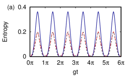
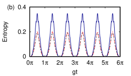
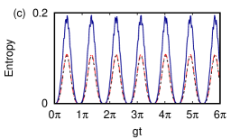
Figure 1: $\xi_{\textsc{tei}}$ (black dashed curve), $\xi^{\prime}_{\textsc{tei}}$ (blue solid curve) and $0.1\,\xi_{\textsc{qmi}}$ (red dot-dashed curve) versus scaled time $gt$ for the field subsystem in the double JC model. (a) $\Delta=0$, initial state $\ket{0;0;\phi_{0}}$  (b) $\Delta=0$, initial state $\ket{0;0;\psi_{0}}$  (c) $\Delta=1$, initial state $\ket{0;0;\psi_{0}}$.

Figs. 2 (a)-(c) depict plots of $\xi_{\textsc{tei}},\xi^{\prime}_{\textsc{tei}}$ and $\xi_{\textsc{qmi}}$ corresponding to the atomic subsystem for the same set of parameters and initial states as in Figs. 1. In this case, although $\xi_{\textsc{tei}}$ is in good agreement with $\xi_{\textsc{qmi}}$ over the time interval considered, $\xi^{\prime}_{\textsc{tei}}$ is not, in sharp contrast to the situation for the field subsystems. We note that when $\Delta=0$, $\xi_{\textsc{qmi}}$ returns to its initial value of $2$ at the instant $gt=\pi$. We will use this feature in the sequel, when we construct an equivalent circuit for the double JC model.

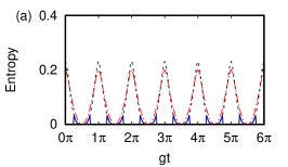
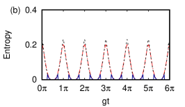
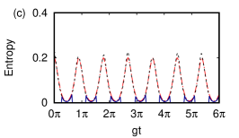
Figure 2: $\xi_{\textsc{tei}}$ (black dashed curve), $\xi^{\prime}_{\textsc{tei}}$ (blue solid curve) and $0.1\,\xi_{\textsc{qmi}}$ (red dot-dashed curve) versus $gt$ for the atomic subsystem in the double JC model. (a) $\Delta=0$, initial state $\ket{0;0;\phi_{0}}$  (b) $\Delta=0$, initial state $\ket{0;0;\psi_{0}}$  (c) $\Delta=1$, initial state $\ket{0;0;\psi_{0}}$.

The equivalent circuit from which bipartite qubit tomograms are obtained (analogous to the tomograms corresponding to the atomic subsystem of the double JC model) is shown in Fig. 3. We use the standard notation of the IBM platform ibm_main , as the circuit has been implemented experimentally and simulated numerically using IBM Q. In the circuit, $q[0]$ and $q[4]$ are the qubits that follow the dynamics of the atomic subsystem while $q[2]$ and $q[3]$ act as auxiliary qubits to aid the dynamics. Since transitions between the two energy levels of either atom in the double JC model involve absorption or emission of a single photon, each auxiliary qubit in the equivalent circuit toggles between the qubit states $\ket{0}$ and $\ket{1}$ respectively. Here

$$U_{3}(\theta,\varphi,\chi)=\begin{bmatrix}\cos\,(\theta/2)\;&\;\;-e^{i\chi}\,\sin\,(\theta/2)\\[4.0pt] e^{i\varphi}\,\sin\,(\theta/2)\;&\;\;e^{i(\chi+\varphi)}\,\cos\,(\theta/2)\end{bmatrix},$$ (15)

where $0\leqslant\theta<\pi,\,0\leqslant\varphi<2\pi$ and $0\leqslant\chi<2\pi$. Each of the four qubits is initially in the qubit state $\ket{0}$. The initial entangled state between $q[0]$ and $q[4]$ (analogous to the initial state $\ket{\psi_{0}}$ of the atomic subsystem) is prepared in the circuit using an Hadamard and a controlled-NOT gate between $q[4]$ and $q[2]$ and a SWAP gate between $q[2]$ and $q[0]$. Here, $\theta$ is analogous to $gt$ in the double JC model. We choose $\theta=\pi$, $\varphi=0$ and $\chi=\pi/2$. As noted earlier, the extent of entanglement is equal to its initial value ($=2$) if $\theta=\pi$, and the values of $\varphi$ and $\chi$ are set for implementation of the circuit. The matrix $U_{3}(\pi,\pi/2,\pi)$ which appears in the equivalent circuit is equal to $U_{3}^{\dagger}(\pi,0,\pi/2)$.

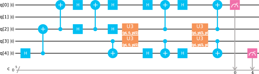
Figure 3: Equivalent circuit diagram for the double JC model (created using IBM Q).

Measurements are carried out in the $x$, $y$ and $z$ bases. A measurement in the $x$-basis is achieved by applying an Hadamard gate followed by a $z$-basis measurement. (The measurement in the $z$-basis is automatically provided by the IBM platform). Defining the operator

$$S^{\dagger}=\begin{bmatrix}1&0\\ 0&-i\end{bmatrix},$$ (16)

measurement in the $y$-basis is achieved by applying $S^{\dagger}$, then an Hadamard gate, and finally a measurement in the $z$-basis. Measurements in the $x$, $y$ and $z$ bases are needed for obtaining the spin tomogram, Fig. 4 (a). (This is equivalent to the bipartite atomic tomogram in the double JC model, in the basis sets of $\sigma_{x}$, $\sigma_{y}$ and $\sigma_{z}$).

These spin tomograms have been obtained experimentally using the IBM superconducting circuit with appropriate Josephson junctions (Fig. 4 (a)), and the QASM simulator provided by IBM which does not take into account losses at various stages of the circuit (Fig. 4 (b)). These tomograms are compared with the atomic tomograms (Fig. 4 (c)) of the double JC model with decoherence effects neglected.

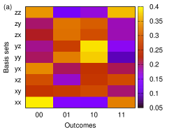
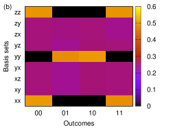
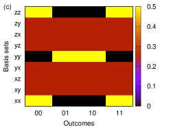
Figure 4: Tomograms obtained by (a) experimental realization (b) simulation of the equivalent circuit (c) simulation of the double JC model.

The qualitative features are very similar in Figs. 4 (b) and (c) as the circuit follows the dynamics of the atomic subsystem of the double JC model. As expected, Fig. 4 (a) is distinctly different.

From these tomograms, we have calculated the corresponding tomographic entanglement indicator $\xi_{\textsc{tei}}$. The values obtained from the experiment, simulation and numerical analysis are $0.0410\pm 0.0016$, $0.2311$ and $0.2310$, respectively. In the first case, tomograms were obtained from six executions of the experiment (each execution is $8192$ runs over each of the 9 basis sets), and the error bar was calculated from the standard deviation of $\xi_{\textsc{tei}}$. Owing to losses at various stages of the experiment, $\xi_{\textsc{tei}}$ is significantly smaller than the value expected from simulation of the circuit and from the JC model.

It is instructive to estimate the extent of loss in state preparation alone. For this purpose, an entangled state of two qubits was prepared using an Hadamard and a controlled-NOT gate, to effectively mimic $\ket{\psi_{0}}$. Tomograms were obtained experimentally in six trials as before, and $\xi_{\textsc{tei}}$ computed from these. They were compared with corresponding values from numerical simulation of the entangled state and from the atomic tomogram corresponding to $\ket{\psi_{0}}$. These values are $0.0973\pm 0.0240$, $0.2310$ and $0.2310$ from the experiment, simulation and numerical analysis respectively. This demonstrates that substantial losses arise even in state preparation. In order to examine the extent to which an increase in the number of atoms in the system increases these losses, we turn to the double Tavis-Cummings (TC) model.

3.2 The double Tavis-Cummings model

The model comprises four two-level atoms, $C_{1}$, $C_{2}$, $D_{1}$ and $D_{2}$, with $C_{1}$ and $C_{2}$ (respectively, $D_{1}$ and $D_{2}$) coupled with strength $g$ to a radiation field $A$ (respectively, $B$) of frequency $\omega$. The effective Hamiltonian (setting $\hbar=1$) is dtcm

$$H_{\textsc{DTC}}=\sum_{j=A,B} \omega\,a_{j}^{\dagger}a_{j}+\sum_{k=1}^{2}\big{\{}\tfrac{1}{2}\omega_{0}\,\sigma_{\textsc{c}_{k}z}+\tfrac{1}{2}\omega_{0}\,\sigma_{\textsc{d}_{k}z}$$

$$+g(a_{\textsc{a}}^{\dagger}\sigma_{\textsc{c}_{k}-}+a_{\textsc{a}}\sigma_{\textsc{c}_{k}+})+g(a_{\textsc{b}}^{\dagger}\sigma_{\textsc{d}_{k}-}+a_{\textsc{b}}\sigma_{\textsc{d}_{k}+})\big{\}},$$ (17)

where the notation is self-explanatory. Initially, $C_{1}$ and $D_{1}$ (respectively, $C_{2}$ and $D_{2}$) are considered to be in a bipartite entangled state. This state could either be $\ket{\psi_{0}}$ (Eq. 13) or $\ket{\phi_{0}}$ (Eq. 14). Each field is initially in $\ket{0}$. We consider three initial states of the full system, namely, $\ket{0;0;\psi_{0};\psi_{0}}$, $\ket{0;0;\phi_{0};\phi_{0}}$ and $\ket{0;0;\psi_{0};\phi_{0}}$. The notation $\ket{0;0;\psi_{0};\phi_{0}}$ indicates, for instance, that $A$ and $B$ are in the state $\ket{0}$, the bipartite subsystem $(C_{1},D_{1})$ is in the state $\ket{\psi_{0}}$, and the bipartite subsystem $(C_{2},D_{2})$ is in the state $\ket{\phi_{0}}$. For brevity, we refer to the bipartite atomic subsystems $(C_{1},C_{2})$ and $(D_{1},D_{2})$ as subsystems $C$ and $D$, respectively.

An equivalent circuit for the double TC model will require 4 qubits to mimic the four two-level atoms together with a minimum of 4 auxiliary qubits to aid the dynamics. In order to assess the extent of losses in state preparation alone, 4 qubits were prepared in a pairwise entangled state (analogous to the initial state $\ket{\psi_{0};\psi_{0}}$ of the atomic subsystem $(C,D)$) using $2$ Hadamard and $2$ controlled-NOT gates (Fig. 5). Here qubits $q[2]$ and $q[3]$ are entangled with qubits $q[0]$ and $q[4]$ respectively. As in the earlier case, tomograms have been obtained (a) experimentally using the IBM quantum computer, (b) from the QASM simulator, and (c) from the corresponding atomic tomogram for $\ket{\psi_{0};\psi_{0}}$. Note that the pair ($q[2]$,$q[3]$) is analogous to subsystem $C$, and ($q[0]$,$q[4]$) is analogous to $D$. We have calculated the extent of entanglement $\xi_{\textsc{tei}}$ between the two $2$-qubit subsystems. The numerical values obtained from (a), (b) and (c) are $0.2528$, $0.4761$ and $0.4621$, respectively. As 4 qubits are involved in this circuit, the number of possible outcomes is 16. (Recall that the number of outcomes in the earlier case was 4.) The maximum number of experimental runs possible in both cases is 8192ibm_main . Hence, the experimental losses, as well as the difference between the simulated and the numerically obtained values, are higher than those obtained for the double JC model. We therefore proceed to investigate the entanglement dynamics of the double TC model numerically in the absence of losses.

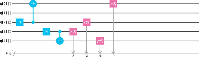
Figure 5: Circuit for preparing an entangled state analogous to $\ket{\psi_{0};\psi_{0}}$ (created using IBM Q).

We have investigated the entanglement between the field subsystems $A$ and $B$, and between the atomic subsystems $C$ and $D$, as the system evolves in time. For this purpose, we have numerically generated the states of the full system and the corresponding tomograms during temporal evolution, at 300 instants separated by a time step 0.02 in units of $\pi/g$. From these, we have obtained the two entanglement indicators $\xi_{\textsc{tei}}$ and $\xi^{\prime}_{\textsc{tei}}$ as functions of time. These indicators and the corresponding $\xi_{\textsc{qmi}}$ between $A$ and $B$ are plotted in Figs. 6 (a)-(c). (Here, the detuning parameter may be set equal to zero, without loss of generality.) $\xi_{\textsc{tei}}$, $\xi^{\prime}_{\textsc{tei}}$ and $\xi_{\textsc{qmi}}$ corresponding to entanglement between $C$ and $D$ are plotted in Figs. 7 (a)-(c).

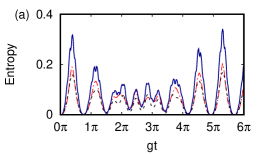
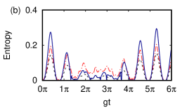
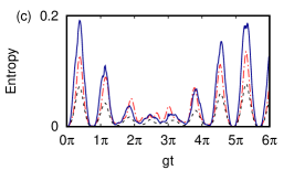
Figure 6: $\xi_{\textsc{tei}}$ (black dashed curve), $\xi^{\prime}_{\textsc{tei}}$ (blue solid curve) and $\xi_{\textsc{qmi}}/10$ (red dot-dashed curve) between the two radiation fields $A$ and $B$ versus time $gt$ with $\Delta=0$. The fields are in the initial state in $\ket{0;0}$, while the atoms are in (a) $\ket{\psi_{0};\psi_{0}}$  (b) $\ket{\phi_{0};\phi_{0}}$  (c) $\ket{\psi_{0};\phi_{0}}$.

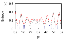
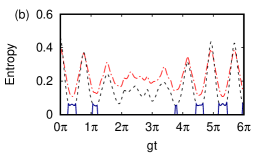
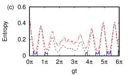
Figure 7: $\xi_{\textsc{tei}}$ (black dashed curve), $\xi^{\prime}_{\textsc{tei}}$ (blue solid curve) and $\xi_{\textsc{qmi}}/10$ (red dot-dashed curve) between the two atomic subsystems $C$ and $D$ versus $gt$ with $\Delta=0$. The initial states of the fields and atoms are the same as in Figs. 6 (a)-(c).

The inferences drawn from the double JC model are seen to hold good in this case too: namely, that both the indicators effectively mimic $\xi_{\textsc{qmi}}$ for the field subsystem, while $\xi^{\prime}_{\textsc{tei}}$ does not reflect $\xi_{\textsc{qmi}}$ for the atomic subsystem.

4 Concluding remarks

We have compared an entanglement indicator $\xi_{\textsc{tei}}$ obtained directly from tomograms, and an approximation to it ($\xi^{\prime}_{\textsc{tei}}$), with the quantum mutual information $\xi_{\textsc{qmi}}$, in the case of the double JC and the double TC models. In both models, the approximation is satisfactory for the field subsystem, but not for the atomic subsystem. $\xi_{\textsc{tei}}$, however, is found to be a good estimate in both models and for both subsystems. This would imply that a good entanglement indicator could be obtained directly from tomograms, circumventing error-prone and lengthy procedures of state reconstruction in multipartite hybrid systems involving field-atom interactions. An equivalent circuit for the double JC model was both experimentally run and numerically simulated to obtain entanglement indicators. This facilitates the estimation of experimental losses and establishes that the results from the IBM simulator agree well with numerical simulation of the double JC model. By constructing equivalent circuits for state preparation in both models, we have shown that the difference in the values of the entanglement indicator obtained experimentally and numerically increases significantly with an increase in the number of atoms.

- (1) T. Yu, J. Eberly, Science 323, 598 (2009)
- (2) Z.X. Man, Y.J. Xia, N.B. An, Eur. Phys. J. D. 53, 229 (2009)
- (3) W. Vogel, R.L.d.M. Filho, Phys. Rev. A 52, 4214 (1995)
- (4) F. Deppe, M. Mariantoni, E. Menzel, A. Marx, S. Saito, K. Kakuyanagi, H. Tanaka, T. Meno, K. Semba, H. Takayanagi, et al., Nat. Phys. 4, 686 (2008)
- (5) A. Retzker, E. Solano, B. Reznik, Phys. Rev. A 75, 022312 (2007)
- (6) P. Laha, B. Sudarsan, S. Lakshmibala, V. Balakrishnan, Int. J. Theor. Phys. 55, 4044 (2016)
- (7) P. Laha, S. Lakshmibala, V. Balakrishnan, J. Opt. Soc. Am. B 36, 575 (2019)
- (8) X. Li, J. Shang, H.K. Ng, B.G. Englert, Phys. Rev. A 94, 062112 (2016)
- (9) M. Rohith, C. Sudheesh, J. Opt. Soc. Am. B 33, 126 (2016)
- (10) B. Sharmila, K. Saumitran, S. Lakshmibala, V. Balakrishnan, J. Phys. B: At. Mol. Opt. 50, 045501 (2017)
- (11) B. Sharmila, S. Lakshmibala, V. Balakrishnan, Quantum Inf. Process. 18, 236 (2019)
- (12) L. Lamata, A. Parra-Rodriguez, M. Sanz, E. Solano, Adv. Phys. X 3, 1457981 (2018)
- (13) IBM Q: Documentation and support. https://quantum-computing.ibm.com/support
- (14) Qiskit: An Open-source Framework for Quantum Computing. https://qiskit.org
- (15) K. Vogel, H. Risken, Phys. Rev. A 40, 2847 (1989)
- (16) A. Ibort, V.I. Man’ko, G. Marmo, A. Simoni, F. Ventriglia, Phys. Scripta 79, 065013 (2009)
- (17) A.I. Lvovsky, M.G. Raymer, Rev. Mod. Phys. 81, 299 (2009)
- (18) R.T. Thew, K. Nemoto, A.G. White, W.J. Munro, Phys. Rev. A 66, 012303 (2002)