Recovering Localized Adversarial Attacks

Recovering Localized Adversarial Attacks

Abstract

Deep convolutional neural networks have achieved great successes over recent years, particularly in the domain of computer vision. They are fast, convenient, and – thanks to mature frameworks – relatively easy to implement and deploy. However, their reasoning is hidden inside a black box, in spite of a number of proposed approaches that try to provide human-understandable explanations for the predictions of neural networks. It is still a matter of debate which of these explainers are best suited for which situations, and how to quantitatively evaluate and compare them [1]. In this contribution, we focus on the capabilities of explainers for convolutional deep neural networks in an extreme situation: a setting in which humans and networks fundamentally disagree. Deep neural networks are susceptible to adversarial attacks that deliberately modify input samples to mislead a neural network’s classification, without affecting how a human observer interprets the input. Our goal with this contribution is to evaluate explainers by investigating whether they can identify adversarially attacked regions of an image. In particular, we quantitatively and qualitatively investigate the capability of three popular explainers of classifications – classic salience, guided backpropagation, and LIME – with respect to their ability to identify regions of attack as the explanatory regions for the (incorrect) prediction in representative examples from image classification. We find that LIME outperforms the other explainers.

1 Introduction

In recent years, deep learning has led to astonishing achievements in several domains, including gaming, machine translation, speech processing, and computer vision [2]. The deep neural networks involved act mostly as black boxes, and as a result they are often met with a certain wariness, especially in safety-critical environments, matters where fairness is important, or when rigorous explanations of a decision are legally required. A number of approaches have been proposed which aim to explain the decisions of neural networks to human users. They include methods that determine particularly relevant input regions for a certain decision, methods that locally approximate complex decisions via human-understandable sparse surrogates, classifier visualization techniques, or more general methods that supplement automated decisions by a notion of their domain of expertise, and explicit reject options whenever their validity is questionable [3, 4, 5, 6].

Explainers need to address two contradictory goals: they need to preserve the explained (highly nonlinear) model’s behavior as much as possible, but simplify it such that it becomes accessible to humans in the form of an explanation. In practice, it is unclear in how far established explainers master this compromise. One problem is that, given an input and a prediction, it is not necessarily clear what a correct explanation for the prediction should look like, because the ground truth of which features truly influence the network’s prediction is unknown. It might be tempting to judge explanatory methods on whether they succeed in identifying features that a human observer thinks should be relevant to the classification, but the existence of adversarial examples shows that the reasoning of humans and neural networks can differ dramatically. In this contribution, we exploit the existence of adversarial examples, using localized adversarial attacks to construct pairs of inputs and predictions together with ground-truth information about which image pixels determine the prediction of the network.

Adversarial attacks are an unsolved challenge for deep neural networks – and more generally for black-box approaches that aim to classify high-dimensional data as is present in computer vision. These attacks result in adversarial examples, which are deliberately generated to fool a classifier. Depending on the specifics of the attack, it may or may not not be recognizable by humans, with noticeable artifacts being produced in some cases [7]. In any case, a proper adversarial attack modifies a given input in such a way that the attacked neural network estimates a different (wrong) label, while a human user would assign the same label to the modified input as to the original input.

In this contribution, we use adversarial examples as an extreme setting in which we can investigate the capabilities of explainers with regards to what makes an input adversarial. In other words, we want to understand how adversarial attacks affect explanations of predictions of deep neural networks and make use of them to produce ground-truth explanations, which allows a quantitative evaluation of explainers. For this we explain adversarial attacks in Section 2. Then, we take a look at three popular explainers for neural networks in Section 3, namely:

• classic salience [8] maps, which are based on gradients propagated through a neural network

• guided backpropagation [9], which also takes into account the representations that are implicitly learned by neural networks, and

• LIME [4], which locally approximates the usually highly nonlinear neural network by a sparse, linear, human-understandable surrogate model.

In Section 4, we define the setting and evaluate the behavior of these methods within the field of computer vision: we quantitatively evaluate in how far methods that explain the decision of deep neural networks can locate where an adversarial attack has modified an image. We finish with a conclusion in Section 5.

(a)

(b)

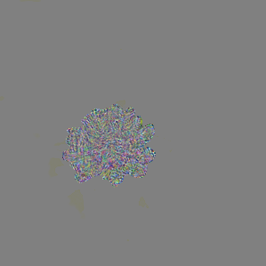
(c)

Figure 1: An adversarial attack: The original image (a) is classified flower. After a localized adversarial attack is performed the resulting adversarial example (b) is classified wolf spider. The difference (c) between the two images is seemingly random noise. It is confined to one of the blossoms in the image.

2 Adversarial Attacks

Given a classifier $f$, a sample $x$ and a label $y=f(x)$ that $f$ assigns to $x$, the goal of an adversarial attack is to modify $x$ just enough such that $f$ assigns a different label $z$ to the modified sample $x^{\prime}$, where $z\neq y$ can be any other label (in which case the attack is called untargeted) or a specific label (in which case the attack is called targeted). In the simplest setting, $f$ is known to the attacker in its entirety. Black-box attacks, on the other hand, attack deep networks without requiring access to $f$ itself. Instead, they use a surrogate that is inferred from a representative training set. In this work we assume that $f$ is available. Commonly, an untargeted attack on a sample $x$ is formalized as the optimization problem

$$\min\lVert x^{\prime}-x\rVert\quad\text{such that}\quad f(x^{\prime})\neq f(x),x^{\prime}\in C(x),$$ (1)

where $C$ denotes additional constraints on the adversarial example $x^{\prime}$, such as box constraints or sparsity. Early approaches aim for an optimization of this problem by standard solvers such as LBFGS, while more recent approaches vary the objective and optimization strategies; software suites available include foolbox [10] and cleverhans [11].

For our evaluation, we need to efficiently perform targeted adversarial attacks constrained to varying regions within a number of different input images. This process yields adversarial examples together with ground truth as to which region in an example is responsible for its (mis-)classification. We use a targeted, iterative variant of the Fast Gradient Sign Method (FGSM) [12], the Basic Iterative Method (BIM) [13]. BIM, just as FGSM, relies on the fact that adversarial attacks can be observed also for linear mappings in high dimensional input spaces. Based on this rationale, attacks move an input $x$ along a linear approximation of the objective $J(x,y)$ of the network, adding the change $\epsilon\cdot\mathrm{sign}[\nabla_{x}J(x,y)]$.

Localized attacks

We want to investigate whether an explanation can identify the attack as the reason for the prediction of the neural network. For this purpose, we use a modified version of BIM, a localized attack [7], for which a quantitative evaluation of the question, whether an explainer identified the right region, is straightforward: we implement an additional constraint $C(x)$ by allowing $x^{\prime}$ to deviate from the original input image $x$ only in a specified region of $x$. This enables us to evaluate the explanation of the resulting adversarial example by measuring the overlap of the pixels (i. e. features) that constitute the explanation with those within the attack region.

3 Explaining Predictions

There exist different methods to explain predictions as produced by black-box mechanisms such as deep networks. Explanations can be either local for the decision $f(x)$ for input $x$, or they can be global for the function $f$. They typically focus on either features or prototypes as the basic “language” to explain the model. Here, we are interested in explaining adversarial examples generated by changing a limited number of features. Hence, we focus on local explanations of $f(x)$ where $x$ is an adversarial example, and use for methods that provide a set of features which best explain this decision. Our quantitative evaluation of the results relies on the overlap of features which we changed during generation of an adversarial example $x$, and the set of features that are used to explain the decision $f(x)$. We compare three different local explanation strategies with respect to their ability in identifying the features where attacks have taken place.

Classic Salience

Salience maps were proposed e. g. by [8] as a visual feedback about the most relevant regions of an image for a specific classification. Essentially, an input feature $x_{i}$ is highlighted according to its relevance for the classification as given by the gradient $\partial J(x,y)/\partial x_{i}$.

Guided Backpropagation

One of the reasons for the success of deep convolutional networks is attributed to their ability to learn higher level feature representations of the object as represented within the activation of the hidden layers [14]. A plain gradient as used for salience maps does not focus on these features because it propagates back both positive and negative contributions of the gradients. Guided backpropagation [9] circumvents this problem by truncating negative gradients during backpropagation.

LIME

[4] proposed Local Interpretable Model-agnostic Explanations (LIME) as an agnostic method that does not use the specific form of the classifying function $f$ that it explains. It tries to approximate the function $f$ locally around $x$ by an interpretable surrogate in the form of a sparse model in features $\tilde{x}_{i}$ derived from $x$. For this purpose, examples are generated around $x$ by jittering, and labeled according to $f$. The resulting training set is used to infer a sparse, explainable, linear model, which describes $f$ locally around $x$. For image classification, the basic features $\tilde{x}_{i}$ are typically superpixels, which are obtained from a perceptual grouping of the image pixels.

4 Experimental Evaluation

We evaluate the information which is provided by these explanations about adversarial attacks for the popular deep neural network Inception v3 [15] as provided by pytorch’s torchvision package. We are interested in two research questions:

R1

Is it possible to uncover substantial information about the location of adversarial attacks in an image by means of explainers?

R2

If the answer is yes, are there substantial differences with regards to the effectiveness of different explanation strategies as introduced above?

Generating adversarial examples

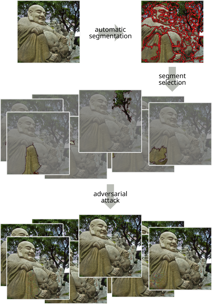
Figure 2: Overview of our process of generating multiple adversarial examples via localized adversarial attacks from a single input image. First, the image is automatically segmented. Then, the largest segments are chosen and individually used to constrain an adversarial attack.

(a)

(b)

(c)

(d)

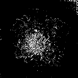
(e)

(f)

Figure 3: Partial explanations for the adversarial example from Figure 1 for classic salience (d), guided backpropagation (e), and LIME (f). (c) is the ground truth. White indicates pixels relevant for the classification. All explanations contain the same number of white pixels.

To guarantee that our test images were not part of the attacked network’s training set, we use crops of $112$ images that we took ourselves. For each attack, we set the constraint $C(x)$ such that only a relatively small region within the input image is modified. We obtain those regions by automatic segmentation using the graph-based algorithm proposed by [16] – during this process, semantics are not explicitly taken into account, and regions are instead constructed based on color statistics. When a region contains exactly one object, the attack can resemble the replacement of said object – to illustrate this, we manually segment a small number of input images, e. g. the one seen in Figure 1. Out of every original input image we generate up to 10 adversarial examples via BIM restricted to the 10 largest regions (cf. Figure 2). The same target label wolf spider is used for every attack. If an attack is not successful or ceases to progress after a certain number of iterations, we discard the attempt. In total, we produce $608$ adversarial examples. With this setup we can guarantee that there exist different regions of the same image, which are attacked and should be uncovered, i.e. finding the location of an attack is a non-trivial task, which is not already determined by the image itself.

Evaluation of Explanations

We explain each adversarial example using Classic Salience, Guided Backpropagation, and LIME. LIME segments the adversarial example into disjoint superpixels and ranks those by their influence on the prediction. We look at the $20$ most influential superpixels $S_{1},\dots,S_{20}$ and see how well the partial union $\mathop{{\bigcup}}_{i=1}^{n}S_{i}$ for $n=1,\dots,20$ recovers the constraint region $C$. For Classic Salience and Guided Backpropagation we sort the pixels in the adversarial example by the $\ell_{1}$ norm of the respective gradients, i. e. by their influence on the prediction. In order to compare the results to those produced by LIME, we look at the $\left|\mathop{{\bigcup}}_{i=1}^{n}S_{i}\right|$ pixels with the highest influence (cf. Figure 3). In total, we compare $12\,160$ explanations for each of the three explainers.

To determine how well such a set of pixels $P$ recovers the region $C$ we calculate the Jaccard Index of the two sets

$$J(P,C)=\frac{P\cap C}{P\cup C}$$ (2)

and a likeness

$$H(P,C)=1-\frac{\mathop{\text{Ham}(P,C)}}{N}$$ (3)

which we base on the Hamming distance between $P$ and $C$ interpreted as binary masks over the entire image with $N$ pixels in total. Both values are between zero and one, with one indicating a perfect match.

LIME distinguishes between superpixels that strongly contribute towards a certain prediction and those that strongly oppose it. We only take into account the former, and in order to interpret the salience maps accordingly, we discard negative gradients in the input layer before we calculate the gradients’ magnitudes.

Results

Table 1: Mean ranks for all three explainers over all $12\,160$ explanations with respect to the Jaccard index and the Hamming-based likeness. $1.0$ is best, $3.0$ is worst.

	Mean rank
Explainer	Jaccard	Hamming
Classic salience	2.58	2.59
Guided backprop	2.06	2.03
LIME	1.36	1.38

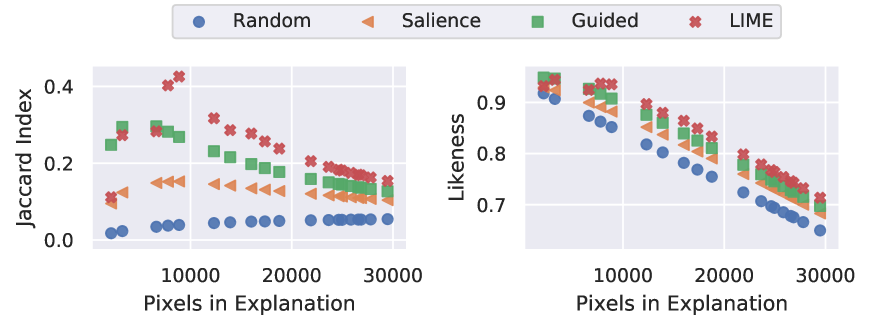
Figure 4: Jaccard index and Hamming-based likeness for different explanation sizes for the adversarial example from Figure 1.

When we compare the explanations provided by LIME with the ground truth, if for a certain $n\in\{1,\dots,20\}$ the partial union $\mathop{{\bigcup}}_{i=1}^{n}S_{i}$ contains all ground-truth pixels, larger unions can only perform worse. We see this in Figure 4, where the best Jaccard index is reached early for a relatively small number of pixels in the explanation. Classic salience and guided backpropagation behave comparably. To demonstrate that the obtained values are indeed meaningful, we include a random baseline – selecting pixels at random yields a very low Jaccard index.

Note that the default segmentation algorithm inside LIME differs from the one we use to automatically determine regions we attack. Hence, it is almost impossible for LIME to achieve perfect scores.

To compare all three explainers with regards to the entire $608$ adversarial examples, we rank them according to the Jaccard index and Hamming index for each example from $1$ (best) to $3$ (worst). The mean ranks are listed in Table 1. LIME outperforms the other two methods, even though those are based on gradients, just as the adversarial attacks.

All explainers include pixels outside the ground-truth region in their explanations. This is especially noticable for LIME, where entire contiguous segments are selected. This is to be expected, because the neural network’s prediction is reached considering the entire input image. Our attacks only change the prediction from one label to a different one. Pixels outside the attacked region can still contribute to both.

5 Conclusion

The results in Section 4 allow us to answer the initial two research questions:

R1

All three tested explanation techniques detect a substantial part of the region where adversarial attacks have taken place which is clearly better than random.

R2

Explanation methods that focus on semantics rather than mere gradients, as offered by guided backpropagation and LIME, perform distinctly better in the tested settings.

The latter finding is particularly interesting in the sense that saliency is essentially based on the same information, which also guides adversarial attacks, namely gradient information. Still, LIME or truncated gradient, both relying on simplifying assumptions, result in a better recovering of the regions where attacks have taken place.

We have investigated the behavior of explanatory methods for deep learning when confronted with adversarial examples. We found that semantics-based approaches in particular are able to identify a substantial part of regions in which an attack has taken place, for a representative set of samples.

In general, we desire a better understanding of adversarial attacks, robustness against them, the certainty of predictions and their explanations, and of how deep convolutional neural networks divide the input space into class regions. With this work, we contribute but a small step towards a more comprehensive grasp of these interlinked concepts. Understanding how labels relate to each other might allow us to construct ground truth with a clearer distinction between strongly and weakly relevant pixels, so that pixels outside attacked regions do not contribute to the prediction as much. Unfortunately, current state-of-the-art classifiers ignore semantic similarities between classes.

Our findings support the idea that it is possible to recover regions that are – by design – the cause for incorrect (adversarial) classifications. In subsequent work we will investigate whether our findings generalize to alternative classification methods and whether explanations of adversarial examples display systematic differences when compared to explanations of proper (correctly classifiable) samples. Furthermore, we will produce an extension towards an interactive scenario in which a human user is aided in understanding principles and pitfalls of automated classification.

References

- [1] Sina Mohseni, Niloofar Zarei and Eric D. Ragan “A Survey of Evaluation Methods and Measures for Interpretable Machine Learning”, 2018 arXiv:1811.11839
- [2] Jürgen Schmidhuber “Deep Learning in Neural Networks: An Overview” In Neural Networks 61 Elsevier, 2015, pp. 85–117 DOI: 10.1016/j.neunet.2014.09.003
- [3] Lydia Fischer, Barbara Hammer and Heiko Wersing “Optimal local rejection for classifiers” In Neurocomputing 214, 2016, pp. 445–457 DOI: 10.1016/j.neucom.2016.06.038
- [4] Marco Túlio Ribeiro, Sameer Singh and Carlos Guestrin ““Why Should I Trust You?”: Explaining the Predictions of Any Classifier” In Proceedings of the 22nd ACM SIGKDD International Conference on Knowledge Discovery and Data Mining, 2016 DOI: 10.18653/v1/n16-3020
- [5] Wojciech Samek, Thomas Wiegand and Klaus-Robert Müller “Explainable Artificial Intelligence: Understanding, Visualizing and Interpreting Deep Learning Models”, 2017 arXiv:1708.08296
- [6] Alexander Schulz, Andrej Gisbrecht and Barbara Hammer “Using Discriminative Dimensionality Reduction to Visualize Classifiers” In Neural Processing Letters 42, 2014, pp. 27–54 DOI: 10.1007/s11063-014-9394-1
- [7] Jan Philip Göpfert, Heiko Wersing and Barbara Hammer “Adversarial attacks hidden in plain sight”, 2019 arXiv:1902.09286
- [8] Ramprasaath R. Selvaraju et al. “Grad-CAM: Visual Explanations from Deep Networks via Gradient-Based Localization” In IEEE International Conference on Computer Vision (ICCV), 2017, pp. 618–626 DOI: 10.1109/iccv.2017.74
- [9] Jost Tobias Springenberg et al. “Striving for Simplicity: The All Convolutional Net”, 2014 arXiv:1412.6806
- [10] Jonas Rauber, Wieland Brendel and Matthias Bethge “Foolbox: A Python toolbox to benchmark the robustness of machine learning models”, 2017 arXiv:1707.04131
- [11] Nicolas Papernot et al. “Technical Report on the CleverHans v2.1.0 Adversarial Examples Library”, 2016 arXiv:1610.00768
- [12] Ian J. Goodfellow, Jonathon Shlens and Christian Szegedy “Explaining and Harnessing Adversarial Examples”, 2014 arXiv:1412.6572
- [13] Alexey Kurakin, Ian J. Goodfellow and Samy Bengio “Adversarial Machine Learning at Scale”, 2016 arXiv:1611.01236
- [14] Yoshua Bengio, Aaron C. Courville and Pascal Vincent “Representation Learning: A Review and New Perspectives” In IEEE Transactions on Pattern Analysis and Machine Intelligence 35, 2013, pp. 1798–1828
- [15] Christian Szegedy et al. “Rethinking the Inception Architecture for Computer Vision” In IEEE Conference on Computer Vision and Pattern Recognition (CVPR), 2016, pp. 2818–2826 DOI: 10.1109/cvpr.2016.308
- [16] Pedro F. Felzenszwalb and Daniel P. Huttenlocher “Efficient Graph-Based Image Segmentation” In International Journal of Computer Vision 59, 2004, pp. 167–181 DOI: 10.1023/b:visi.0000022288.19776.77