Graphene under bichromatic driving: Commensurability and spatio-temporal symmetries

Abstract

We study the non-linear current response of a Dirac model that is coupled to two time-periodic electro-magnetic fields with different frequencies. We distinguish between incommensurable and commensurable frequencies, the latter characterized by $\Omega_{2}=(p/q)\Omega_{1}$ with co-prime integers $p$ and $q$. Coupling the (effective) two-level system to a dissipative bath ensures a well-defined long-time solution for the reduced density operator and, thus, the current. We then analyze the spatio-temporal symmetries that force certain current components to vanish and close with conclusions for directed average currents.

1 Introduction

Driven systems are ubiquitous in solid-state physicsGrifoni1998a ; Forster2015b ; Kohler2005a , and recently their relation to emergent topological phases has attracted much attention Kitagawa10 ; Lindner11 ; Gu11 ; Jiang11 ; Gomez13 ; Cayssol13 . Remarkably, a non-trivial Berry curvature can also induce a temporal phase transition if the driving is sufficiently strong Rudner19 and driving protocols can further be extended to quantum dot arrays that might be used as quantum simulators for 1D topological phases PerezGonzalez19 . This opens up new possibilities for manipulating states of matter via strong external, time-periodic fields. For a two-level system with Chern number $C$, a quantized energy pumping with rate $(C/2\pi)\omega_{1}\omega_{2}$ can then occur if the two frequencies $\omega_{1}$ and $\omega_{2}$ are incommensurable Martin17 .

An established technique for treating ac driven systems beyond linear response is Floquet theory which is usually employed for simple harmonic time-dependences. Nevertheless, multi-frequency driving with incommensurable frequencies can be treated as well, but requires a multi-dimensional Floquet lattice Hanggi1998a . Moreover, one can map such quasi-periodic systems to periodic systems leading to Floquet time spirals Zhao19 .

In this paper, we shall investigate a two-level system driven by two frequencies that may be commensurable as well as incommensurable. The system is further coupled to a dissipative decay channel which leads to a master equation description for the reduced dynamics. Its long-time solution provides the time averaged current. We are then interested in analyzing the symmetries of the system that lead to a vanishing current.

The creation of directed currents by purely oscillating forces has a long history in classical Brownian motion, where it is known as ratchet effect Reimann2002a ; Hanggi2009a . It has been studied also in the quantum realm Reimann1997a ; Lehmann2002b . Generally, ratchet effects stem from an interplay of non-linearities and ac driving that brings the system out of equilibrium such that detailed balance is broken. Symmetries that inhibit the ratchet effect usually take the shape of the driving as a function of time into account, i.e., they are of spatio-temporal nature Flach2000a ; Reimann2001a . Lately, such concepts have been developed also in the context of Floquet topological insulators Peng2019a .

The paper is organised as follows: In Sec. 2, we will introduce the Dirac model and Chern number and relate the two-level system to various physical systems. In Sec. 3, we will then outline the master equation and the Floquet techniques for its solution. In Sec. 4, we discuss the conditions for a vanishing current in a certain direction and in Sec. 5, we present the numerical results resolved in $k$-space. We close with conclusions and final remarks.

2 Model

2.1 Graphene in two electromagnetic fields

The motivation of this work is to discuss the non-linear current response of graphene, but in order to simplify the general discussion, we will constrain ourselves to only one valley. The Hamiltonian is thus given by (in units with $\hbar=v_{F}=e=1$)

$$H_{0}({\vec{k}})=\vec{k}\cdot{\vec{\sigma}}+m\sigma_{z},\quad{\vec{\sigma}}=\begin{pmatrix}\sigma_{x}\\ \sigma_{y}\end{pmatrix}\;,$$ (1)

with the gap parameter $m$ and the quasi momentum $\vec{k}$ measured relatively to the $K$-point.

Via minimal coupling, two orthogonal driving fields are introduced as the time-dependent Hamiltonians

$$H_{1}(t)={} a_{1}\sigma_{x}\cos(\Omega_{1}t),$$ (2)

$$H_{2}(t)={} a_{2}\sigma_{y}\cos(\Omega_{2}t+\theta),$$ (3)

where the frequency ratio $\Omega_{2}/\Omega_{1}$ may be irrational or rational, i.e., equal to $p/q$ with co-prime integers $p$ and $q$. Without loss of generality, we allow for a phase shift in the second field, only.

The total Hamiltonian thus reads $H(t)=H_{0}+H_{1}(t)+H_{2}(t)$, and we assume that for a chemical potential at the Dirac point, the two single-particle states for a given momentum $\vec{k}$ are fully occupied and empty, respectively, such that the current density reads

$$\vec{j}=\frac{1}{A}\sum_{\vec{k}}\langle{\vec{\sigma}}\rangle=\frac{1}{4\pi^{2}}\int d^{2}k\,\langle\vec{\sigma}\rangle\;,$$ (4)

where $\langle\vec{\sigma}\rangle$ denotes the time-averaged expectation value.

For a realistic description of many-body effects, this one-particle approach may represent a severe limit. However, within the present work we restrict ourselves to analyzing the spatio-temporal symmetries of single-particle states in an idealized situation.

2.2 General two-level systems and Chern number

Our approach can be applied to any two-level system and the general Hamiltonian defined on a two-dimensional torus would read

$$H={\vec{g}}({\vec{k}})\cdot{\vec{\sigma}}\;.$$ (5)

For ${\vec{g}}({\vec{k}})=(\tau k_{x},k_{y},m)$, this reduces to the Dirac Hamiltonian, i.e., single-valley gapped graphene with $\tau=\pm$ denoting the different valleys Neto09 ; Xiao10 . As already said, this Hamiltonian will be treated in detail below.

For ${\vec{g}}({\vec{k}})=(k_{x}^{2}-k_{y}^{2},2\tau k_{x}k_{y},\Delta)$, we would model biased bilayer graphene Li10 , resembling one of the first examples of topological edge states localized in the region for which a sign change in the bias voltage occursMartin08 . Setting ${\vec{g}}({\vec{k}})=(v_{x}\sin(k_{x}),v_{y}\sin(k_{y}),m-b_{1}\cos(k_{x})-b_{2}\cos(k_{y}))$, one obtains a half of the BHZ model Bernevig06 . The last version was discussed in Ref. Martin17 after coupling it to two independent driven fields.

The Chern number of a two-level system in two dimension can be defined as

$$C=\frac{1}{4\pi}\int d^{2}k\ \hat{\vec{g}}\cdot(\partial_{k_{x}}\hat{\vec{g}}\times\partial_{k_{y}}\hat{\vec{g}})\;,$$ (6)

with $\hat{\vec{g}}={\vec{g}}/|{\vec{g}}|$. For gapped graphene, $C=\tau\mathop{\mathrm{sgn}}(m)$, while for biased bilayer $C=\tau\mathop{\mathrm{sgn}}(\Delta)$ and for the half BHZ model we have a quantum Hall insulator with $C=\pm 1$ for $-|b_{1}|-|b_{2}|<m<-||b_{1}|-|b_{2}||$ and $||b_{1}|-|b_{2}||<m<|b_{1}|+|b_{2}|$, respectively.

Coupling the graphene Hamiltonian to a circularly polarized light field

$$H_{\mathrm{circ}}(t)=g(\sigma_{+}e^{i\Omega_{1}t}+\sigma_{-}e^{-i\Omega_{1}t})$$ (7)

may lead to non-trivial topological properties, i.e., for the Dirac Hamiltonian, we obtain $C=\mathop{\mathrm{sgn}}(m+g)$ for $\tau=+$ and $C=-\mathop{\mathrm{sgn}}(m-g)$ for $\tau=-$ Cayssol13 . The net Chern number can thus become non-trivial even after including both valleys if the coupling is sufficiently strong or the gap sufficiently small, i.e., $|g|\geq|m|$.

In addition to the Chern, we could also calculate the more general dynamical conductivity tensor defined as

$$\sigma_{nm}(\omega)=\frac{1}{\omega}\int_{0}^{\infty}e^{i\omega t}\langle[j_{n}(t),j_{m}(0)]\rangle\;,$$ (8)

with $n,m=x,y$. In the static limit $\omega\rightarrow 0$, we then have the relation

$$\sigma_{xy}=\frac{e^{2}}{2\pi\hbar}C\;,$$ (9)

where we have restored SI-units for the moment. The above equation resembles the main result of the celebrated integer Hall effect Klitzing80 ; Thouless82 ; Streda82 .

In the following, we will go beyond linear response theory and discuss the current in the non-linear regime. As a special case, we also analyze the dynamical Hall response.

3 Long-time solution

3.1 Quantum dissipation

To obtain a well-defined steady state, we introduce a weak dissipation mechanism. To this end, one may start from a system-bath model to obtain an equation of motion for the reduced density operator of the dissipative system. Then one can show that generally dissipation is quantitatively affected by the driving Kohler1997a ; Grifoni1998a . Here, however, we are interested in the generic response to bichromatic driving and we will follow a less involved path which allows an efficient numerical solution for rather long propagation times. Therefore, we simply employ a Lindblad master equation for the density operator Breuer2003a , $\dot{\rho}=-i[H_{0}+H_{1}+H_{2},\rho]+\gamma\mathcal{D}(\rho)$ with the Lindblad dissipator Breuer2003a

$$\mathcal{D}(\tilde{\sigma}_{-})\rho=\tilde{\sigma}_{-}\rho\tilde{\sigma}_{+}^{\dagger}-\frac{1}{2}\tilde{\sigma}_{+}^{\dagger}\tilde{\sigma}_{-}\rho-\frac{1}{2}\rho\tilde{\sigma}_{+}^{\dagger}\tilde{\sigma}_{-},$$ (10)

where $\tilde{\sigma}_{-}=|\varphi_{0}\rangle\langle\varphi_{1}|$ is the ladder operator in the eigenbasis of $H_{0}$ which maps the excited state to the ground state.

3.2 Solution of the master equation

For time-dependent master equations of this type, the time-averaged long-time solution of the density operator can be obtained with Floquet methods, both in the commensurable and the incommensurable case. In the following, we sketch the underlying ideas and for details refer the reader to Ref. Forster2015b .

3.2.1 Commensurable frequencies

For $\Omega_{2}=(p/q)\Omega_{1}$, with co-prime $p$ and $q$, the system is periodic with a fundamental frequency $\Omega=\Omega_{1}/q$. Then, since the master equation is linear and (generally) ergodic, $\rho(t)$ becomes $2\pi/\Omega$ periodic after a transient stage and can be written as a Fourier series

$$\rho(t)=\sum_{k}e^{-ik\Omega t}\rho_{k}.$$ (11)

Inserting this Floquet ansatz into the master equation and choosing a suitable cutoff for the Fourier index $k$, yields a set of linear equations for the coefficients $\rho_{k}$ which we solve numerically. We are finally interested in the time average over one period given by $\rho_{0}$.

3.2.2 Incommensurable frequencies

For incommensurable frequencies, i.e., for irrational values of $\Omega_{2}/\Omega_{1}$, one may decompose the long-time solution of $\rho(t)$ into a two-dimensional Fourier series, one for each frequency Hanggi1998a ; Chu2004a . This however may lead to rather large sets of equations which are hard to solve numerically. For a more efficient treatment, we employ a method Forster2015b based on the combination of the Floquet decomposition explained above, the $t$-$t^{\prime}$ formalism Peskin1993a , and matrix-continued fractions Risken .

The method starts by replacing one time argument in the Liouvillian by $t^{\prime}$ to obtain the modified master equation

$$\Big{(}\frac{\partial}{\partial t}+\frac{\partial}{\partial t^{\prime}}\Big{)}R(t,t^{\prime})=\mathcal{L}(t,t^{\prime})R(t,t^{\prime})$$ (12)

with

$$\mathcal{L}(t,t^{\prime})=L_{0}+L_{1}\cos(\Omega_{1}t)+L_{2}\cos(\Omega_{2}t^{\prime}+\theta).$$ (13)

It can be shown straightforwardly that when $R(t,t^{\prime})$ is a solution of Eq. (13), then $R(t,t^{\prime})|_{t^{\prime}=t}$ solves the original master equation Peskin1993a . Practically, one treats the additional time $t^{\prime}$ (or equivalently, some angle $\alpha=\Omega_{2}t^{\prime}$) as additional canonical coordinate with conjugate momentum $i\partial/\partial t$.

For Eq. (13), the ansatz

$$R(t,t^{\prime})=\sum_{k,n}e^{-ik\Omega_{1}t}e^{-in\Omega_{2}t^{\prime}}r_{k,n}\,,$$ (14)

yields a set of equations which is tri-diagonal in both indices, $k$ and $n$. It is solved by writing the dependence on one index as a Floquet matrix like in Sect. 3.2.1 while the dependence on the other index is expressed as a recurrence relation that can be solved by matrix-continued fractions. The latter numerical method scales only linearly with the cutoff index, which makes the method considerably more efficient than the direct matrix representation of the two-frequency decomposition. Finally, we obtain the coefficient $r_{0,0}$ which contains the full information about the long-time average of $\rho(t)$.

It has been shown Forster2015b that $r_{0,0}$ does not depend on the relative phase of the drivings, $\theta$. This is indeed expected from physical intuition, because for quasi-periodic driving fields, any relative phase between the two ac signals can be mapped to a time translation which should not affect long-time averages. Below we derive this phase independence more formally within a symmetry analysis.

4 Spatio-temporal symmetries

The first term of the time-independent Hamiltonian $H_{0}$, i.e., $\vec{k}\cdot\vec{\sigma}$, is given by a inner product which is invariant under time-reversal (which changes the sign of both $\vec{k}$ and $\vec{\sigma}$) and under a rotation around the $z$-axis. However, as $m$ and $\sigma_{z}$ are not components of a vector, a rotation around any other axis does not correspond to a transformation in real space. Nevertheless, such rotations may be symmetry operations for $H(t)$ and must be considered. For this reason, we treat in our symmetry analysis $\vec{k}$ as well as the driving amplitudes $a_{1,2}$ as parameters that are not affected by the transformations. Notice that this does not imply any restriction, because a possible sign in $k_{x}$ or $k_{y}$ is irrelevant for the integral in Eq. (4), while possible minus signs of the amplitudes can be absorbed by the relative phase of the driving fields.

The principal observable for our setup is the current density $\vec{j}$ which is given by an integral of the time-averaged expectation value $\langle\vec{\sigma}\rangle$, see Eq. (4). Thus, whenever a component of this quantity possesses some anti-symmetry as a function of $\vec{k}$, the corresponding current component will vanish. The aim of this section is a symmetry analysis of $H(\vec{k},t)$ in the spirit of Refs. Flach2000a ; Reimann2001a that reveals under which conditions one or both current components are symmetry forbidden. In doing so, we consider spatio-temporal transformations that map $H(\vec{k},t)$ to some $H(\vec{k}^{\prime})$, where $\vec{k}$ and $\vec{k}^{\prime}$ are related by a mirror or point symmetry. The spatial part of the mapping is formally a rotation or inversion in three-dimensions with the corresponding transformation of the Pauli matrices.

4.1 Commensurable frequencies

4.1.1 Periodicity in the phase $\theta$

Before considering transformations of Pauli matrices, let us derive for later use a symmetry property for the phase $\theta$ of the driving defined in Eq. (3). Obviously, $H_{2}(t)$ is $2\pi$ periodic in $\theta$. In the long-time limit, however, time-averaged expectation values as a function of $\theta$ possess a higher symmetry, namely a $2\pi/q$ periodicity which we derive in the following.

As already mentioned above, for rational $\Omega_{2}/\Omega_{1}=p/q$, the Hamiltonian is periodic in time. Then after a transient stage, the density operator $\rho(t)$ generally assumes the same time periodicity, and so does any expectation value of a time-independent observable. Hence, all averages over one driving period are invariant under time translations. We are now interested in phase transformations $\theta\to\theta+\Delta\theta$ with a $\Delta\theta$ that can be absorbed into a time translation $\tau$, such that averages over one driving period remain invariant.

From the definition of $H_{2}(t)$, we immediately see that such a phase shift corresponds to a time translation by $\tau=\Delta\theta/\Omega_{2}$. This, in turn, provides for the driving $H_{1}$ a phase shift $\Delta\theta\Omega_{1}/\Omega_{2}=\Delta\theta q/p$. Whenever this phase is a multiple of $2\pi$, $\Delta\theta$ will not affect stationary expectation values. This is the case for $\Delta\theta=2\pi p\ell/q$, where $\ell$ may be any integer.

We choose $\ell=p^{\varphi(q)-1}$, with $\varphi$ being Euler’s totient function which counts the natural numbers up to $q$ that are co-prime to $q$. As 1 is considered co-prime to all natural numbers, $\varphi(q)\geq 1$ which ensures that the chosen $\ell$ is an integer number. As $p$ and $q$ are co-prime, Euler’s theorem states that $p^{\varphi(q)}\equiv 1\mod q$. Hence, for the present choice,

$$\Delta\theta=\frac{2\pi}{q},$$ (15)

which implies the to be demonstrated $2\pi/q$ periodicity of time-averaged expectation values.

4.1.2 Temporal symmetries of the driving shape

Next we consider the time dependent functions in the driving Hamiltonians $H_{1,2}(t)$ given by

$$f_{1}(t)={} \cos(q\Omega t),$$ (16)

$$f_{2}(t)={} \cos(p\Omega t+\theta).$$ (17)

We are interested in transformations that change the sign of at least one of these functions and accordingly classify them by $\vec{s}=(s_{1},s_{2})$ with $s_{i}=\pm$. For the cosine, two transformations come to mind. First, a time translation and, second, time-reversal at times that correspond to zeros of $f_{1,2}$. Importantly, due to the periodicity worked out above, we have the freedom to change $\theta$ by any multiple of $2\pi/q$ without affecting the time-averaged response.

Time translation

The first option is the mapping $t\to t+\tau$, where $\tau$ will be determined such that $f_{1}$ acquires a sign $s_{1}$. Thus, $\tau=2\pi\ell/q\Omega$ for $s_{1}=+$ and $\tau=\pi(2\ell+1)/q\Omega$ for $s_{1}=-$, where $\ell$ is an arbitrary integer. The corresponding condition on $f_{2}$ reads

$$\cos(p\Omega t+\theta)=s_{2}\cos(p\Omega t+p\Omega\tau+\theta^{\prime})$$ (18)

and must be fulfilled for all $t$, while $\theta^{\prime}\equiv\theta\pmod{2\pi/q}$ owing to the aforementioned $2\pi/q$ periodicity. Inserting the already determined values of $\tau$ straightforwardly leads to the conditions summarized in the first line of Table 1. Notice that a minus sign in $f_{2}$, i.e. a phase $\pi$, can be absorbed by $\theta^{\prime}$ provided that $q$ is even.

Time reversal

As $t$ enters as argument of the cosines, its sign is irrelevant for $f_{1}$. For $f_{2}$, the mapping $t\to-t$ is equivalent to changing the sign of $\theta$. Allowing again also an additional time translation and a phase shift by a multiple of $2\pi/q$, the most general time inversion reads $(t,\theta)\to(t+\tau,-\theta^{\prime})$. Then, $f_{1}$ is not affected such that we find for $\tau$ the same possible values as above. The difference lies in the minus sign in front of $\theta^{\prime}$ such that for $\vec{s}=(-+)$, the condition on the arguments of $f_{2}$ becomes

$$\theta\equiv\frac{\pi p}{q}(2\ell+1)-\theta\mod\frac{2\pi}{q},$$ (19)

where we have used $\theta\equiv\theta^{\prime}\pmod{2\pi/q}$. Thus, $\theta$ no longer disappears from the symmetry condition, but for even $q$ must be $\theta\equiv 0\pmod{\pi/q}$. For odd $q$, it is restricted to $\theta\equiv\pi/2q\pmod{\pi/q}$. Notice the absence of the factor $2$ in the modulus. The conditions for $\vec{s}=(-+)$ and $\vec{s}=(--)$ are evaluated in the same manner and provide the second and third line of Table 1.

Table 1: Symmetries of the driving under time translation $t\to t+\tau$ and time reversal $t\to-(t+\tau)$. The signs of the driving shapes $f_{1}(t)=\cos(q\Omega t)$ and $f_{2}(t)=\cos(p\Omega t+\theta)$ change as indicated in the first line provided that $p$, $q$, and $\theta$ obey the conditions listed in the subsequent lines. Notice that as $p$ and $q$ are co-prime by assumption, $p+q$ is even only when both $p$ and $q$ are odd.

Sign change $\vec{s}$ of $f_{1}$, $f_{2}$	$+-$	$-+$	$--$
Time translation	$q$ even	$p$ even	$p+q$ even
Time reversal, $\theta=0$	$q$ even	$p$ even	$p+q$ even
Time reversal, $\theta=\pi/2q$	$q$ odd	$p$ odd	$p+q$ odd

4.1.3 Transformation of the Pauli matrices

The spatial part consists of the usual behavior of Pauli matrices under rotation and time reversal Sakurai . Due to the fact that a symmetry transformation must not mix the couplings to the ac drivings (unless $\Omega_{1}=\Omega_{2}$, the only possibilities are transformations that change the sign of one or several Pauli matrices. They are given by combinations of rotations at the coordinate axis by an angle $\pi$ and time reversal, where all $2^{3}-1$ possibilities (the identity is not relevant for our purpose) are listed in the top row of Table 2.

Let us once more emphasize that we consider the momentum $\vec{k}$ and the amplitudes $a_{1}$, $a_{2}$ as mere parameters, such that $T$ only acts on the (pseudo)-spin space and the arguments of the cosines. Their action on the Pauli matrices is displayed in the second row of Table 2.

Table 2: Spatio-temporal symmetries for which the current $\vec{j}=(j_{x},j_{y})$ or one of its components are zero. They include all possible combinations the time-reversal $T$ and rotations $R_{i}$ by an angle $\pi$ at the coordinate axes $i=x,y,z$. The conditions on the phase $\theta$ are modulo $\pi/q$ and, thus, in the range $[0,2\pi)$ are fulfilled $2q$ times. The last two columns list the most relevant symmetries as for those the entire current vanishes. The mapping via $TR_{z}$ solely affects $\sigma_{z}$ which is not linked to any current.

Symmetry operation	$TR_{x}$	$TR_{y}$	$TR_{z}$	$R_{x}$	$R_{y}$	$R_{z}$	$T$
Signature, impact on $\sigma_{x},\sigma_{y},\sigma_{z}$	$-++$	$+-+$	$++-$	$+--$	$-+-$	$--+$	$---$
Restrictions:
– gap			$m=0$	$m=0$	$m=0$		$m=0$
– frequency ratio $\Omega_{2}/\Omega_{1}=p/q$				$q$ even	$p$ even	$p,q$ odd
– phase $\theta\pmod{\pi/q}$	$\begin{cases}0&\text{$p$ even}\\ \frac{\pi}{2q}&\text{$p$ odd}\end{cases}$	$\begin{cases}0&\text{$q$ even}\\ \frac{\pi}{2q}&\text{$q$ odd}\end{cases}$					$\begin{cases}0&\text{$p+q$ even}\\ \frac{\pi}{2q}&\text{$p+q$ odd}\end{cases}$
Consequence for current	$j_{x}=0$	$j_{y}=0$		$j_{y}=0$	$j_{x}=0$	$\vec{j}=\vec{0}$	$\vec{j}=\vec{0}$

4.1.4 Combining both transformations

Armed with the knowledge of the previous subsections, we are in the position to analyze the spatio-temporal symmetries of our problem. Notably, the spatial transformations in Table 2 invert the sign of at least one Pauli matrix. Then, under the conditions listed in Table 1, there exists a time transformation that restores the original sign of the driving Hamiltonians $H_{1}$ and $H_{2}$. Thus, the combination of both transformations maps $H(\vec{k})$ to some $H(\vec{k}^{\prime})$ with $\vec{k}^{\prime}=(\pm k_{x},\pm k_{y})$. Therefore owing to the integration in Eq. (4), a current component $j_{i}$ vanishes if the transformation inverts the sign of $\sigma_{i}$.

An important point is that $\sigma_{z}$ does not couple to any driving field nor does it depend on the momentum. Therefore, any mapping that involves $\sigma_{z}\to-\sigma_{z}$ can be a symmetry operation only in the gapless case $m=0$.

As an example, let us consider a $\pi$-rotation around the $z$ axis, which maps $H_{0}(\vec{k})$ to $H_{0}(-\vec{k})$ and $H_{1,2}(t)\to-H_{1,2}(t)$. According to the last column of Table 1, there exists for even $p+q$ (i.e., $p,q$ both odd) a time translation that restores the sign of both drivings. Therefore, we can conclude that the momenta $\vec{k}$ and $-\vec{k}$ are symmetry related. As both $\sigma_{x}$ and $\sigma_{y}$ have changed their sign, the contributions of these momenta to the current $\vec{j}$ cancel each other. Thus, the current is symmetry forbidden. Let us remark that this case represents the most important symmetry: first, because both current components vanish and, second, as it holds also in the gapped case.

Generally, for any spatial transformation, one has to look at Table 1 for a time transformation with the same signature (ignoring the last one which corresponds to $\sigma_{z}$), such that the driving Hamiltonians remains invariant. Then all $\sigma_{i}$ that change their sign possess some anti-symmetry in $\vec{k}$ space. Hence, $j_{i}=0$. The conditions under which a proper time transformation exists can be read off from Table 1 and provide the restrictions on $p$, $q$, and $\theta$ displayed in Table 2.

Notice that in some cases, a symmetry may represent a special case of a higher symmetry. For example, time reversal symmetry $T$ predicts for the gapless case $m=0$ and $p+q\equiv 0\mod{2}$ (implying that both $p$ with $q$ are odd) a vanishing current for particular values of $\theta$. For this case, however, the rotation around the $z$-axis is less restrictive and leads to the same conclusion for any phase and even for a finite gap.

4.1.5 Generalization of the Hamiltonian

Rotation around the $z$ axis, $R_{z}$, as well as time reversal $T$ have in common that both Pauli matrices relevant for the current, $\sigma_{x}$ and $\sigma_{y}$, transform in the same way. Therefore, in the driving Hamiltonians we may replace $\sigma_{x}$ and $\sigma_{y}$ by any linear combination of the two without loosing the corresponding symmetry properties. Physically, this means that the polarization of the two incident electric fields need not be orthogonal, but may have any orientation in the $x$-$y$ plane. Interestingly, this property holds true precisely for those symmetries for which both current components vanish.

For the other symmetries (besides for $TR_{Z}$ which does not have consequences for the current), this generalization is not possible, because the spatial part of the transformation changes the sign of only one of the two Pauli matrices that define the current.

4.2 Incommensurable frequencies

For irrational $\Omega_{2}/\Omega_{1}$, the system always possesses the highest symmetry that can be achieved in the commensurable case. This can be understood as follows. The symmetry analysis for the commensurable case is based on the compensation of a prefactor $-1$ in the driving by a proper time transformation. For an arbitrary frequency $\Omega_{1}$, the sign of $H_{1}$ can be inverted by a time translation $t\to t+\pi(2\ell+1)/\Omega_{1}$ with an arbitrary integer $\ell$. Then, the phase in $H_{2}$ effectively changes by

$$\Delta\theta=\pi\frac{\Omega_{2}}{\Omega_{1}}(2\ell+1)\mod 2\pi.$$ (20)

If $\Omega_{2}/\Omega_{1}$ is irrational, one can always choose $\ell$ such that it brings $\Delta\theta$ arbitrarily close to its original value (or to any other desired values, e.g., to $\pi$ if one wishes to establish a minus sign). By contrast, for $\Omega_{2}/\Omega_{1}=p/q$ with $p,q$ being co-prime, the possible phase shifts can assume only $q$ different values.

Notice that this argument silently assumes that the average is computed over an infinitely large time. Therefore, it will be difficult to distinguish in an experiment an incommensurable case from a commensurable case with rather large $p$ and $q$.

The arguments used in Sec. 4.1.5 for the generalization of the driving also hold here. Therefore, also for incommensurable frequencies, we can replace in $H_{1}$ and $H_{2}$ the Pauli matrices by any linear combination of $\sigma_{x}$ and $\sigma_{y}$ without loosing the symmetry properties that lead to a point symmetry of $\langle\sigma_{x,y}\rangle$ with respect to the origin of $k_{x}$-$k_{y}$ plane and, thus, to a vanishing current density.

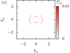
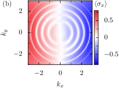
Figure 1: (a) Excitation probability as function of the momentum $\vec{k}$ for driving frequencies $\Omega_{2}=2\Omega_{1}$ and equal amplitudes $a_{1}=a_{2}=0.01$ within the linear response regime. (b) Time-averaged $\langle\sigma_{x}\rangle$ for monochromatic driving $\Omega_{2}=\Omega_{1}$ with a phase $\theta=\pi/2$ that corresponds to circular polarization. The much larger amplitudes $a_{1}=a_{2}=3$ create a response dominated by higher harmonics. For illustrative purposes, the dissipation rate is chosen rather large, $\gamma=0.05$.

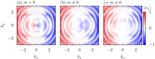
Figure 2: Expectation value $\langle\sigma_{x}\rangle$ as a function of momentum $\vec{k}$ for the resonance $p/q=2/3$ with $\Omega_{1}=1$. (a) In the absence of a gap ($m=0$) for the phase $\theta=\pi/2q$. (b) For a gap $m=0.5$ and phase $\theta=\pi/2q$. (c) For a gap $m=0.5$ and phase $\theta=0$. The amplitudes are $a_{1}=a_{2}=3$, while the dissipation rate is $\gamma=10^{-3}$.

4.3 Hall response

By setting one driving field to zero, we can also discuss the possibility of a non-linear Hall response of the system, i.e., we are looking for a current in, say, $y$-direction if the external driving field is applied in $x$-direction.

One might expect some non-trivial response in the case of a finite gap, but since there is only one driving field, the highest possible symmetry is attained by the system. The highest symmetry class is also represented by both $p$ and $q$ odd and we infer from Table 2 that the total current is always zero and thus no non-linear Hall current can be generated. This is true for any finite frequency and there is thus no dynamical Hall effect induced by non-linear radiation.

5 Numerical results

Besides the current densities $j_{x,y}$, our main quantity of interest are the time-averaged expectation values of the Pauli matrices $\sigma_{x,y}$ as a function of $\vec{k}$. Both are linked by the integral in Eq. (4). Physical insight may also be provided by the probability of finding the system in the excited state. To compute the latter, we determine the excited state $|\phi_{1}\rangle$ of the undriven $H_{0}(\vec{k})$ (the index $\vec{k}$ in the energies and eigenstates is suppressed). Then we evaluate $P_{\text{ex}}=\langle\phi_{1}|\rho_{\infty}|\phi_{1}\rangle$, where $\rho_{\infty}$ in the one-period average of the density operator or, in the incommensurable case, its long-time average.

5.1 Commensurable frequencies

To set the stage, we first consider the excitation probability for bichromatic driving with small amplitudes, such that the parameters stay within the linear response limit, see Figure 1a. As is characteristic for linear response, there emerge two independent excitations, one for each driving frequency. Their shape as a ring reflects the rotational symmetry of $H_{0}(\vec{k})$. The zeros of the excitations at $k_{x}=0$ and $k_{y}=0$, respectively, are due to the fact that for these momenta, one of the drivings commutes with the bare Hamiltonian $H_{0}$. Hence it cannot cause any excitation. The displayed color-coded intensities are $\propto\cos^{2}\theta$.

Another instructive case is monochromatic driving with circular polarization shown in Figure 1b, but now with a much larger amplitude far beyond linear response. Owing to the equal amplitudes and the circular polarization, the driving still possesses the rotational symmetry of $H_{0}$. An interesting feature is the counter-clockwise smearing, which is a consequence of dissipation. For the opposite circular polarization, the smearing is clockwise (not shown). To make this effect visible, we here used an unphysically large dissipation. In all other figures it is much smaller such that dissipative effects are not significant.

To see how symmetries may be destroyed by the presence of a gap and be restored by choosing a proper phase between the two drivings, let us have a closer look at a resonance with $p/q=2/3$, for zero gap, $m=0$, and phase $\theta=\pi/2q$, see Figure 2. As $p$ is even, according to Table 2, the system has a symmetry whose spatial part consists of a rotation by $\pi$ around the $y$ axis, $R_{y}$. Consequently, the time-averaged $\langle\sigma_{x}\rangle$ as a function of $\vec{k}$ possesses an anti-symmetry by reflection at the $y$ axis which is evident in Figure 2a.

For finite gap (panel b), this symmetry is no longer present. There is also no other symmetry that would affect $\sigma_{x}$. Nevertheless, there is still one symmetry present, namely $TR_{y}$ which implies reflection symmetry of $\sigma_{x}$ at the $x$ axis. Notice, however, that this has no consequences for the current component $j_{x}$, because only anti-symmetries have the effect that the integral in Eq. (4) vanishes. Upon changing the phase to $\theta=0$ (panel c), we find invariance under $TR_{x}$, which for even $p$ has the same consequence as $R_{y}$, which is the mentioned anti-symmetry of $\langle\sigma_{x}\rangle$.

5.2 Incommensurable frequencies

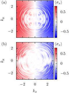
Figure 3: (a) Expectations value $\langle\sigma_{x}\rangle$ for incommensurable frequencies with $\Omega_{2}/\Omega_{1}=(1+\sqrt{5})/2$, i.e., equal to the golden ratio. (b) The same for a modified $H_{2}$ in which $\sigma_{y}$ replaced by $(\sigma_{x}+\sigma_{y})/\sqrt{2}$. The corresponding plots for $\langle\sigma_{y}\rangle$, besides a ration by $90^{\circ}$, look similar and have the same point symmetry.

As a significant example of incommensurable frequencies, we consider a frequency ratio equal to the golden mean, which is considered as the “most irrational number”. The resulting expectation value shown in Figure 3a exhibits many resonance islands without a particular structure. On a rough scale, the excitation probability does not possess any preferential direction despite its lack of rotational symmetry. Nevertheless, as both driving fields are orthogonal to each other, the reflection symmetry at the $k_{x}$ and $k_{y}$ axis remains. For the expectation values of $\sigma_{x}$ and $\sigma_{y}$, this turns into an anti-symmetry. Consequently, after integration over $\vec{k}$ space, the response vanishes as in the case of commensurable frequencies with a particular phase.

Figure 3b depicts the corresponding result when the polarization of the driving $H_{2}$ is rotated by $45^{\circ}$, i.e., when $\sigma_{y}$ is replaced by $(\sigma_{x}+\sigma_{y})/\sqrt{2}$. As expected, then the reflection (anti-) symmetry at the coordinate axis gets lost. Nevertheless, the point anti-symmetry at the origin still holds, thus again leading to $\vec{j}=\vec{0}$.

5.3 Directed average current

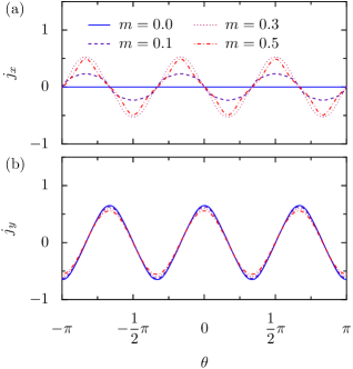
Figure 4: Current for $p/q=2/3$ for various values of the gap. All other parameters are as in Figure 2

Let us now discuss an experimentally accessible quantity namely the dc current. From our symmetry analysis, we have already seen that it must vanish when the system is driven by incommensurable frequencies. The same is true for commensurable frequencies for $\Omega_{2}/\Omega_{1}=p/q$ with both $p$ and $q$ odd. Therefore, we focus on cases with either $p$ or $q$ being even and study the role of the phase $\theta$ between the two driving fields.

We again consider the case $\Omega_{2}/\Omega_{1}=2/3$ for which the time-averaged current is depicted in Figure 4. As $p$ is even, the ungapped case $m=0$ has the symmetry $R_{y}$, such that we expect $j_{x}$ to vanish. In the presence of a gap, we may still have a situation with $TR_{x}$ and $TR_{y}$, which however are symmetries only for certain phases. Since $p$ is even and $q$ odd, the current components $j_{x}$ and $j_{y}$ vanish for $\theta\equiv 0\pmod{\pi/q}$ and for $\theta\equiv\pi/2q\pmod{\pi/q}$, respectively. The numerical data confirm the conjectured appearance of $2q=4$ zeros of each current component. While $j_{y}$ depends only weakly on the gap, the behavior of $j_{x}$ changes significantly. For $m=0$, it vanishes owing to the discussed invariance of $H(t)$ under $R_{y}$. With increasing $m$, $j_{x}$ grows until it reaches the order of magnitude of $j_{y}$. When $p$ and $q$ are interchanged (not shown), the behavior of $j_{x}$ and $j_{y}$ is interchanged as well. The qualitative difference to the former case is that each current component vanishes 6 times since now $q=3$.

We have already argued and seen in Figure 3 that for incommensurable frequencies, the symmetry is always the highest one that we can get in the commensurable case. Therefore, the current will always vanish also beyond linear response and at any order. This summarizes the predominant consequence of incommensurability in our strongly bichromatically driven system.

6 Conclusions

We have analyzed the Dirac model coupled to the radiation of two time-periodic fields with different, possibly incommensurable frequencies. Based on an extensive symmetry analysis, we found that inducing a steady, long-time current requires a frequency ratio $p/q$ with odd $p+q$ (if co-prime). Theoretically, the $q$ different equivalent values of $\theta$ may lie so close to each other that they cannot be resolved experimentally, especially for large $q$. This limits the possibilities for distinguishing in an experiment between commensurable and incommensurable frequencies to clear cases such as the golden ratio or ratios with rather small $p$ and $q$.

Some points have been left open. So far, many-body effects due to the anti-symmetrization of the fermionic wave function have been neglected. Also, in order to address topological quantities more thoroughly, the static limit would have to be performed which can be done within the presented scheme by treating one driving field as perturbation via linear response. These issues raise intriguing questions for further investigations.

- (1) M. Grifoni, P. Hänggi, Phys. Rep. 304, 229 (1998)
- (2) F. Forster, M. Mühlbacher, R. Blattmann, D. Schuh, W. Wegscheider, S. Ludwig, S. Kohler, Phys. Rev. B 92, 245422 (2015)
- (3) S. Kohler, J. Lehmann, P. Hänggi, Phys. Rep. 406, 379 (2005)
- (4) T. Kitagawa, E. Berg, M. Rudner, E. Demler, Phys. Rev. B 82, 235114 (2010)
- (5) N.H. Lindner, G. Refael, V. Galitski, Nature Physics 7, 490 (2011)
- (6) Z. Gu, H.A. Fertig, D.P. Arovas, A. Auerbach, Phys. Rev. Lett. 107, 216601 (2011)
- (7) L. Jiang, T. Kitagawa, J. Alicea, A.R. Akhmerov, D. Pekker, G. Refael, J.I. Cirac, E. Demler, M.D. Lukin, P. Zoller, Phys. Rev. Lett. 106, 220402 (2011)
- (8) A. Gómez-León, G. Platero, Phys. Rev. Lett. 110, 200403 (2013)
- (9) J. Cayssol, B. Dóra, F. Simon, R. Moessner, physica status solidi (RRL) – Rapid Research Letters 7, 101 (2013)
- (10) M.S. Rudner, J.C.W. Song, Nature Physics (2019)
- (11) B. Pérez-González, M. Bello, G. Platero, A. Gómez-León, Phys. Rev. Lett. 123, 126401 (2019)
- (12) I. Martin, G. Refael, B. Halperin, Phys. Rev. X 7, 041008 (2017)
- (13) P. Hänggi, in Quantum Transport and Dissipation (Wiley-VCH, Weinheim, 1998), chap. 5, pp. 249–286
- (14) H. Zhao, F. Mintert, J. Knolle, arXiv:1906.06989 (2019)
- (15) P. Reimann, Phys. Rep. 361, 57 (2002)
- (16) P. Hänggi, F. Marchesoni, Rev. Mod. Phys. 81, 387 (2009)
- (17) P. Reimann, M. Grifoni, P. Hänggi, Phys. Rev. Lett. 79, 10 (1997)
- (18) J. Lehmann, S. Kohler, P. Hänggi, A. Nitzan, Phys. Rev. Lett. 88, 228305 (2002)
- (19) S. Flach, O. Yevtushenko, Y. Zolotaryuk, Phys. Rev. Lett. 84, 2358 (2000)
- (20) P. Reimann, Phys. Rev. Lett. 86, 4992 (2001)
- (21) Y. Peng, G. Refael, Phys. Rev. Lett. 123, 016806 (2019)
- (22) A.H. Castro Neto, F. Guinea, N.M.R. Peres, K.S. Novoselov, A.K. Geim, Rev. Mod. Phys. 81, 109 (2009)
- (23) D. Xiao, M.C. Chang, Q. Niu, Rev. Mod. Phys. 82, 1959 (2010)
- (24) J. Li, A.F. Morpurgo, M. Büttiker, I. Martin, Phys. Rev. B 82, 245404 (2010)
- (25) I. Martin, Y.M. Blanter, A.F. Morpurgo, Phys. Rev. Lett. 100, 036804 (2008)
- (26) B.A. Bernevig, T.L. Hughes, S.C. Zhang, Science 314, 1757 (2006)
- (27) K.v. Klitzing, G. Dorda, M. Pepper, Phys. Rev. Lett. 45, 494 (1980)
- (28) D.J. Thouless, M. Kohmoto, M.P. Nightingale, M. den Nijs, Phys. Rev. Lett. 49, 405 (1982)
- (29) P. Streda, J. Phys. C: Solid State Phys. 15, L717 (1982)
- (30) S. Kohler, T. Dittrich, P. Hänggi, Phys. Rev. E 55, 300 (1997)
- (31) H.P. Breuer, F. Petruccione, Theory of Open Quantum Systems (Oxford University Press, Oxford, 2003)
- (32) S.I. Chu, D.A. Telnov, Phys. Rep. 390, 1 (2004)
- (33) U. Peskin, N. Moiseyev, J. Chem. Phys. 99, 4590 (1993)
- (34) H. Risken, The Fokker-Planck Equation, Vol. 18 of Springer Series in Synergetics, 2nd edn. (Springer, Berlin, 1989)
- (35) J.J. Sakurai, Modern Quantum Mechanics, 2nd edn. (Addison-Wesley, Reading, MA, 1995)