Learning a Generic Adaptive Wavelet Shrinkage Function for Denoising

Abstract

The rise of machine learning in image processing has created a gap between trainable data-driven and classical model-driven approaches: While learning-based models often show superior performance, classical ones are often more transparent. To reduce this gap, we introduce a generic wavelet shrinkage function for denoising which is adaptive to both the wavelet scales as well as the noise standard deviation. It is inferred from trained results of a tightly parametrised function which is inherited from nonlinear diffusion. Our proposed shrinkage function is smooth and compact while only using two parameters. In contrast to many existing shrinkage functions, it is able to enhance image structures by amplifying wavelet coefficients. Experiments show that it outperforms classical shrinkage functions by a significant margin.

Index Terms—  Wavelet Shrinkage, Adaptive Thresholding, Denoising, Interpretable Learning

1 Introduction

With the advent of machine learning, most of the state of the art solutions in image processing tasks have become data-driven: Many degrees of freedom allow a trainable model to adapt well to the input data. While yielding highly tailored solutions, results are often too complex for a rigorous analysis. In contrast to this, classical model-driven approaches provide a sound theoretical foundation but often cannot compete with their learning-based counterparts.

The goal of this work is to combine the advantages of model- and data-driven approaches on the basis of wavelet shrinkage for denoising: Given a signal that has been corrupted by noise, the goal is to reconstruct the original image as well as possible by modifying parts of the signal in the wavelet domain. We exploit the flexibility of a learning-based approach to train a smooth shrinkage function that adapts both to the wavelet scales and to the noise level. The proposed shrinkage function can even amplify wavelet coefficients and thus enhance important image structures, a property that most established shrinkage functions do not share. A low number of trainable parameters allows us to manually inspect the learned results and infer smooth connections between them. From these, we design a generic compact shrinkage function that incorporates the learned adaptivity, while only using two parameters. Experiments show that our shrinkage function outperforms classical ones by a significant margin. To the best of our knowledge, this is the first work to present a learning-based shrinkage function with this level of compactness.

Wavelet shrinkage has first been proposed by Donoho and Johnstone [1]. Therein, a noisy signal is transformed to a wavelet basis, resulting coefficients are modified by a shrinkage function, and then transformed back to obtain a denoised result. Classical shrinkage functions use a single threshold parameter for all scales of the wavelet transformation. However, individual scales might require distinct thresholds as they are differently affected by noise. To this end, adaptive shrinkage methods have been proposed. Early works of Zhang et al. [2, 3] already study a smooth adaptive shrinkage function with trainable thresholds. Other authors train arbitrarily shaped shrinkage functions [4], some also train the wavelets [5] or even general adaptive filters for shrinkage operations [6]. Non-trainable adaptive statistical models include [7, 8]. Most learning-based methods produce large amounts of trained parameters while relations between them are rarely investigated. In contrast to this, we directly employ a tightly parametrised model from which it is easy to infer smooth underlying parameter relations.

An important connection between 2D wavelet shrinkage and nonlinear diffusion filtering has been established by Mrázek and Weickert [9]. It allows us to directly translate a diffusivity into a trainable shrinkage function. We use a so-called Forward-and-Backward (FAB) diffusivity, resulting in a shrinkage function that can amplify coefficients. Only few works employ this property directly [10], but also results for learned shrinkage functions suggest its usefulness [4]. The corresponding concept of backward diffusion has also shown to be successful [11, 12, 13].

The remainder of this paper is structured as follows: In Section 2 we review classical wavelet shrinkage. We propose our model in Section 3, which is experimentally evaluated in Section 4. Finally, Section 5 summarises our conclusions.

2 Classical Wavelet Shrinkage

2.1 Basic Concept

Classical discrete wavelet shrinkage represents a noisy signal $\bm{f}=\bm{v}+\bm{n}$ in the wavelet basis, wherein the additive noise $\bm{n}$ is better separated from the true signal $\bm{v}$. This is achieved by the following three-step framework:

1. Analysis: The input data $\bm{f}$ is transformed to wavelet and scaling coefficients. In this representation, the noise affects all wavelet coefficients while the signal is represented by only a few significant ones [14].

2. Shrinkage: A shrinkage function $S_{\theta}$ with a threshold parameter $\theta$ is applied individually to the wavelet coefficients. The scaling coefficients remain unchanged.

3. Synthesis: The denoised version $\bm{u}$ of $\bm{f}$ is obtained by back-transforming the modified wavelet coefficients.

Many shrinkage functions have been proposed. We will consider the most prominent ones of soft [15], hard [14], and garrote [16] shrinkage for comparison. While these functions are easy to use in a practical setting, they suffer from applying the same threshold parameter to all scales and their binary decision structure. Finer scales might require a different threshold than coarser scales as they are more affected by noise. Furthermore, there is no clear separation between noise and signal coefficients such that eliminating too many coefficients always destroys signal details and eliminating too few leaves noise in the reconstruction.

The classical wavelet transformation is not shift-invariant: Shifting the input signal $\bm{f}$ will produce a different set of wavelet coefficients. To overcome this problem, Coifman and Donoho suggested cycle spinning [17]: The input signal is shifted, wavelet shrinkage is applied, and the results are averaged for all possible shifts. This yields the shift-invariant but redundant non-decimating wavelet transformation.

2.2 Relation to Nonlinear Diffusion

For the two-dimensional wavelet transform, wavelet coefficient channels $w_{x},w_{y}$, and $w_{xy}$ for $x$-, $y$-, and diagonal direction are obtained. To design rotationally invariant shrinkage rules, special care is required. Mrázek and Weickert [9] achieve this by a channel coupling that is inspired by nonlinear diffusion filtering. Their Haar wavelet shrinkage rule is given by

$$S_{\theta}\left(\!\!\begin{pmatrix}w_{x}\\ w_{y}\\ w_{xy}\end{pmatrix}\!\!\right)=\Big{(}1-g\left(w_{x}^{2}+w_{y}^{2}+2\,w_{xy}^{2}\right)\!\!\Big{)}\begin{pmatrix}w_{x}\\ w_{y}\\ w_{xy}\end{pmatrix}\!.$$ (1)

The argument $\,w_{x}^{2}+w_{y}^{2}+2\,w_{xy}^{2}\,$ is a consistent approximation to the rotationally invariant expression $\left|\operatorname*{\bm{\nabla}\!}u\right|^{2}$, where $\left|\,.\,\right|$ is the $L^{2}$ norm and $\operatorname*{\bm{\nabla}\!}=\left(\partial_{x},\partial_{y}\right)^{\top}$ denotes the spatial gradient operator. The function $g$ is a diffusivity function from a nonlinear diffusion filter [18]. In nonlinear diffusion, filtered versions $u(\bm{x},t)$ of an image $f(\bm{x})$ are obtained by solving the partial differential equation

$$\partial_{t}u=\text{div}(g(\left|\operatorname*{\bm{\nabla}\!}u\right|^{2})\operatorname*{\bm{\nabla}\!}u)$$ (2)

with $u(\bm{x},0)=f(\bm{x})$ as initial condition and diffusion time $t$. The diffusivity $g$ steers the activity of the process. It is scalar-valued and becomes small at edges where $\left|\operatorname*{\bm{\nabla}\!}u\right|^{2}$ is large. This results in rotationally invariant edge-preserving denoising.

Mrázek and Weickert [9] have shown that one explicit time step of nonlinear diffusion with diffusivity $g$ is equivalent to coupled Haar wavelet shrinkage (1). Thus, we can directly translate existing diffusivities into shrinkage functions.

3 Trainable Adaptive Wavelet Shrinkage

In our model, we equip the two-dimensional coupled Haar wavelet shrinkage approach from [9] with a trainable adaptive shrinkage function. We sample a noisy image $f$ on a discrete grid with $2^{L}\times 2^{L}$ sampling positions and grid distance $h_{x}=h_{y}=:h$. The discrete image is represented by a vector $\bm{f}$. It is transformed with the non-decimating two-dimensional Haar wavelet transformation $\bm{W}$ into lowpass scaling coefficients at scale $L$ denoted by $\bm{w}^{L}$, and directional wavelet coefficients $\left(\bm{w}_{x}^{\ell},\bm{w}_{y}^{\ell},\bm{w}_{xy}^{\ell}\right)_{\ell=1}^{L}$ for different scales. To ensure that coefficients have the same range on all scales, we rescale the basis functions accordingly. A shrinkage function $S_{\bm{\theta}}$ with parameters $\bm{\theta}=\left(\bm{\theta}^{1},\dots,\bm{\theta}^{L}\right)$ for each scale is applied to the wavelet coefficients. Coefficients on scale $\ell$ are modified component-wise by $S_{\bm{\theta}^{\ell}}$ according to the coupled shrinkage rule (1). We obtain the reconstruction $\bm{u}$ by applying the backward transformation $\bm{\tilde{W}}$ to the modified set of wavelet coefficients and the unaltered scaling coefficients:

$$\bm{u}=\bm{\tilde{W}}S_{\bm{\theta}}\left(\bm{W}\bm{f}\right).$$ (3)

3.1 Choice of Shrinkage Function

We found the Forward-and-Backward (FAB) diffusivity of Smolka [19] to be a good candidate for modelling our shrinkage function. It uses two contrast parameters $\lambda_{1}$ and $\lambda_{2}$ that control the amount of forward and backward diffusion. The diffusivity is given by

$$g(s^{2})=2\,\exp\left(\frac{-s^{2}}{\lambda_{1}^{2}}\right)-\exp\left(\frac{-s^{2}}{\lambda_{2}^{2}}\right),\quad\lambda_{2}\geq\lambda_{1}.$$ (4)

It is translated into the shrinkage function according to the coupled shrinkage rule (1). For the extreme case of $\lambda_{1}=\lambda_{2}$, the diffusivity simplifies to the exponential Perona-Malik diffusivity [18], corresponding to pure shrinkage. For larger differences between $\lambda_{2}$ and $\lambda_{1}$, the backward diffusion becomes more pronounced and the shrinkage function damps small coefficients and amplifies larger ones.

3.2 Learning Framework

To train the shrinkage functions, we add Gaussian noise to a database of ground truth images $\left(\bm{v}_{k}\right)_{k=1}^{K}$. This yields noisy images $\bm{f}_{k}$ from which we compute denoised results $\bm{u}_{k}$. The trainable parameters for the proposed shrinkage function on scale $\ell$ are given by $\bm{\theta}^{\ell}=\left(\lambda_{1}^{\ell},\lambda_{2}^{\ell}\right)$. As an objective function, we choose the mean square error between the reconstruction $\bm{u}_{k}$ and the corresponding ground truth image $\bm{v}_{k}$, averaged over all image pairs and normalised by the number of pixels:

$$E\left(\bm{\theta}\right)=\frac{1}{K}\sum_{k=1}^{K}\frac{\lVert\bm{u}_{k}-\bm{v}_{k}\rVert_{2}^{2}}{2^{2L}}.$$ (5)

The parameters are trained with the gradient-based L-BFGS algorithm [20]. To that end, we compute the gradients of the objective function w.r.t. all trainable parameters.

4 Experiments

In our experimental setup, we use $400$ images from the BSDS500 database [21] as a training set and the $68$ images introduced in [22] as a test set. Their grey values are in $\left[0,255\right]$ and the grid size is set to $h=1$. From each image we select random regions of size $256\times 256$, i.e. the number of scales is $L=8$. All images are corrupted by Gaussian noise of mean 0 and standard deviation $\sigma$. We do not clamp the resulting pixel grey values to the original grey value range to preserve the Gaussian statistics of the noise. We have found the learned parameters to be robust w.r.t. any reasonable initialisation, so no pretraining is performed.

4.1 Evaluation of the Learned Shrinkage Functions

In a first experiment, we train the adaptive shrinkage function for $\sigma=25$. The learned shrinkage functions for different scales are presented in Figure 1. On the first and finest wavelet scale, all coefficients are shrunken. On the second scale, we observe coefficient amplification. We presume that this compensates the loss of image details caused by shrinking coefficients on the first scale. All further scales do not perform significant shrinkage as the learned function approaches the identity. Therefore, we do not display coarser scales $\ell>4$.

Scale 1 (finest)	Scale 2	Scale 3	Scale 4

Fig. 1: Trained shrinkage functions for $\sigma=25$. On fine scales, both shrinkage and amplification are performed. The coarser the scale, the less wavelet coefficients are modified.

When we increase the noise level to $\sigma=50$, we observe that more scales are involved in the shrinkage process. The trained shrinkage functions are displayed in Figure 2. Both configurations are in line with our conjecture that the diffusivity should change smoothly over the scales and the noise levels. Shrinkage and amplification decrease for coarser scales, i.e. $\lambda_{1}^{\ell}$ and $\lambda_{2}^{\ell}$ tend to $0$. With increasing noise, shrinkage and amplification become stronger and affect more scales.

Scale 1 (finest)	Scale 2	Scale 3	Scale 4

Fig. 2: Trained shrinkage functions for $\sigma=50$. With increasing noise, shrinkage becomes more drastic and more scales are involved.

4.2 Ablation Study

To investigate the effectiveness of different aspects of our model, we perform the following ablation study. We start with classical hard wavelet shrinkage and equip it with the non-decimating wavelet transformation and the coupled shrinkage rule to enable a fair comparison. For $\sigma=20$, we obtain an average PSNR on the test set of $27.88$dB. In a second step, we use the proposed shrinkage function restricted to $\lambda_{2}=\lambda_{1}$, so no amplification can take place. Still, the shrinkage function does not adapt to the individual scales. This yields a comparable PSNR of $27.83$dB, showing that smoothness of the shrinkage function alone does not matter for reconstruction quality. When we remove the restriction on the shrinkage function, the PSNR increases to $28.06$dB which indicates that the amplification of wavelet coefficients is helpful for a good reconstruction. Finally, introducing adaptivity to the scales boosts the PSNR to $28.55$dB, demonstrating that the scale dynamic is the crucial ingredient for a good denoising result.

4.3 Finding a Generalised Shrinkage Function

So far, the contrast parameters are trained for each pair of scale $\ell$ and noise level $\sigma$ from which we will now infer a generic relation. Figure 4.3 shows the evolution of both contrast parameters over the scales and the noise levels. A function of type $\frac{\alpha}{\ell^{2}}$ with an appropriate scalar $\alpha$ can provide a good description of the scale dependence of $\lambda_{1}^{\ell}$. For $\lambda_{2}^{\ell}$, the values on fine scales do not follow this relation, but in these cases all relevant coefficients are already covered by shrinkage through a large $\lambda_{1}$, making the choice of $\lambda_{2}$ irrelevant.

Regarding the relationship between the shrinkage functions and the noise standard deviation it was already noted in [4] that a simple rescaling of shrinkage functions is sufficient for adapting to a new noise level. For our parametrisation, rescaling the complete shrinkage function is equivalent to rescaling both $\lambda_{1}$ and $\lambda_{2}$. In Figure 4.3 we can see that indeed such a rescaling is learned.

&

Fig. 3: Relations between trained parameters $\lambda_{1}^{\ell},\lambda_{2}^{\ell}$ and scale $\ell$ (left, middle) and noise level $\sigma$ (right).

These two insights suggest that a suitable generalisation of the shrinkage function parameters which is smooth over the scales $\ell$ and the noise standard deviation $\sigma$ is given by $\lambda_{1}(\ell,\sigma)=\frac{\alpha\sigma}{\ell^{2}}$ and $\lambda_{2}(\ell,\sigma)=\frac{\beta\sigma}{\ell^{2}}$ where $\alpha$ and $\beta$ are scalars that have yet to be determined. To empirically show that this parametrisation indeed captures the underlying relations in a reasonable way, we compare two models: One model trains the proposed shrinkage function for each pair $\left(\ell,\sigma\right)$ individually, while the other one only optimises the factors $\alpha$ and $\beta$ of the generalised parameters. To ensure a fair comparison, both models are trained on a new training and test set combining images with noise levels between $\sigma=10$ and $\sigma=60$ in steps of $2.5$. Indeed, the generic model performs only $0.3$dB worse than the model with individual parameters in terms of PSNR, while training only $2$ instead of $336$ parameters. With this result we conclude that the generic shrinkage function captures the adaptivity to scales and noise levels well. The scalars are learned as $\alpha=5.4$ and $\beta=8.9$, yielding a combined generic coupled shrinkage function (1) with diffusivity

$$g(s^{2},\ell,\sigma)=2\exp\left(\frac{-s^{2}}{\left(\frac{5.4\,\sigma}{\ell^{2}}\right)^{2}}\right)-\exp\left(\frac{-s^{2}}{\left(\frac{8.9\,\sigma}{\ell^{2}}\right)^{2}}\right).$$ (6)

4.4 Comparison to Classical Shrinkage

Lastly, we compare our generic shrinkage function to soft, hard, and garrote shrinkage over a range of noise levels. We optimise the threshold parameter of the classical functions individually for each noise level, while the generic function is used as is from (6). The results are displayed in Figure 4. Although the classical approaches are optimised for each noise level, they are inferior to the generic shrinkage function. Over the range of noise levels used for training, improvements of up to $0.65$dB with an average of $0.34$dB are obtained compared to the best classical approaches.

For $\sigma=50$, Figure 5 shows reconstructions along with the noisy input and the ground truth image. Soft shrinkage blurs the image too strongly since all wavelet coefficients are decreased by the same margin. Hard shrinkage suffers from remaining noise as it does not shrink large noisy wavelet coefficients. While less pronounced, this is also the case for garrote shrinkage. Both garrote and hard shrinkage also blur important image structures. Our generic shrinkage function outperforms all classical approaches. By strongly shrinking coefficients on fine scales, noise is efficiently removed. To compensate for lost image details, amplification of wavelet coefficients on coarser scales enhances important structures.

Fig. 4: PSNR values on the test set (higher is better) for individually optimised classical approaches and our generic shrinkage function. The proposed function outperforms all classical shrinkage functions.

noisy image, PSNR $14.74$dB	soft, PSNR $21.62$dB	hard, PSNR $22.19$dB
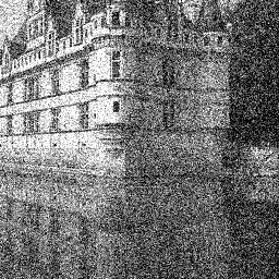
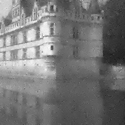
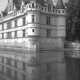
garrote, PSNR $22.10$dB	proposed, PSNR $22.88$dB	ground truth

Fig. 5: Comparison the results of classical shrinkage functions and the generic shrinkage function for $\sigma=50$. For the generic function, the image is significantly less blurred.

5 Conclusions

Our approach of learning a compact shrinkage function for wavelet denoising combines the advantages of model-driven and data-driven approaches: In contrast to other parameter learning strategies, we can cope with as little as two parameters without substantially sacrificing performance. This results in an interpretable shrinkage function and a transparent, but adaptive model.

In our ongoing work we extend these findings to other adaptive nonlinear approaches such as diffusion evolutions.

References

- [1] D. L. Donoho and I. M. Johnstone, “Ideal spatial adaptation by wavelet shrinkage,” Biometrica, vol. 81, no. 3, pp. 425–455, 1994.
- [2] X.-P. Zhang and M. D. Desai, “Nonlinear adaptive noise suppression based on wavelet transform,” in Proc. IEEE International Conference on Acoustics, Speech and Signal Processing, Seattle, WA, May 1998, vol. 3, pp. 1589–1592.
- [3] X.-P. Zhang, “Thresholding neural network for adaptive noise reduction,” IEEE Transactions on Neural Networks, vol. 12, no. 3, pp. 567–584, May 2001.
- [4] Y. Hel-Or and D. Shaked, “A discriminative approach for wavelet denoising,” IEEE Transactions on Image Processing, vol. 17, no. 4, pp. 443–457, Mar. 2008.
- [5] T. Grandits and T. Pock, “Optimizing wavelet bases for sparser representations,” in Energy Minimisation Methods in Computer Vision and Pattern Recognition, M. Pelillo and E. Hancock, Eds., vol. 10746 of Lecture Notes in Computer Science, pp. 249–262. Springer, Cham, 2018.
- [6] U. Schmidt and S. Roth, “Shrinkage fields for effective image restoration,” in Proc. 2014 IEEE Conference on Computer Vision and Pattern Recognition, Columbus, OH, June 2014, pp. 2774–2781.
- [7] S.G. Chang, B. Yu, and M. Vetterli, “Adaptive wavelet thresholding for image denoising and compression,” IEEE Transactions on Image Processing, vol. 9, no. 9, pp. 1532–1546, Sept. 2002.
- [8] J. Portilla, V. Strela, M. J. Wainwright, and E. P. Simoncelli, “Image denoising using scale mixtures of Gaussians in the wavelet domain,” IEEE Transactions on Image Processing, vol. 12, no. 11, pp. 1338–1351, Nov. 2003.
- [9] P. Mrázek and J. Weickert, “From two-dimensional nonlinear diffusion to coupled Haar wavelet shrinkage,” Journal of Visual Communication and Image Representation, vol. 18, no. 2, pp. 162–175, Apr. 2007.
- [10] J.-L. Starck, F. Murtagh, E. Candès, and D. L. Donoho, “Gray and color image contrast enhancement by the curvelet transform,” IEEE Transactions on Image Processing, vol. 12, no. 6, pp. 706–717, June 2003.
- [11] G. Gilboa, N. A. Sochen, and Y. Y. Zeevi, “Forward-and-backward diffusion processes for adaptive image enhancement and denoising,” IEEE Transactions on Image Processing, vol. 11, no. 7, pp. 689–703, Nov. 2002.
- [12] Y. Chen and T. Pock, “Trainable nonlinear reaction diffusion: A flexible framework for fast and effective image restoration,” IEEE Transactions on Pattern Analysis and Machine Intelligence, vol. 39, no. 6, pp. 1256–1272, Aug. 2016.
- [13] M. Welk, J. Weickert, and G. Gilboa, “A discrete theory and efficient algorithms for forward-and-backward diffusion filtering,” Journal of Mathematical Imaging and Vision, vol. 60, no. 9, pp. 1399–1426, Nov. 2018.
- [14] S. Mallat, A Wavelet Tour of Signal Processing, Academic Press, San Diego, second edition, 1999.
- [15] D. L. Donoho, “De-noising by soft thresholding,” IEEE Transactions on Information Theory, vol. 41, pp. 613–627, May 1995.
- [16] H.-Y. Gao, “Wavelet shrinkage denoising using the non-negative garrote,” Journal of Computational and Graphical Statistics, vol. 7, no. 4, pp. 469–488, Dec. 1998.
- [17] R. R. Coifman and D. Donoho, “Translation invariant denoising,” in Wavelets in Statistics, A. Antoine and G. Oppenheim, Eds., pp. 125–150. Springer, New York, 1995.
- [18] P. Perona and J. Malik, “Scale space and edge detection using anisotropic diffusion,” IEEE Transactions on Pattern Analysis and Machine Intelligence, vol. 12, pp. 629–639, July 1990.
- [19] B. Smolka, “Combined forward and backward anisotropic diffusion filtering of color images,” in Pattern Recognition, L. Van Gool, Ed., vol. 2449 of Lecture Notes in Computer Science, pp. 314–320. Springer, Berlin, 2002.
- [20] D. C. Liu and J. Nocedal, “On the limited memory BFGS method for large scale optimization,” Mathematical Programming, vol. 45, no. 1–3, pp. 503–528, Aug. 1989.
- [21] P. Arbelaez, M. Maire, C. Fowlkes, and J. Malik, “Contour detection and hierarchical image segmentation,” IEEE Transactions on Pattern Analysis and Machine Intelligence, vol. 33, no. 5, pp. 898–916, Aug. 2011.
- [22] S. Roth and M. J. Black, “Fields of experts: A framework for learning image priors,” in Proc. 2005 IEEE Conference on Computer Vision and Pattern Recognition, San Diego, CA, June 2005, vol. 2, pp. 860–867.