Sequential Adversarial Anomaly Detection
for One-Class Event Data

Abstract

We consider the sequential anomaly detection problem in the one-class setting when only the anomalous sequences are available and propose an adversarial sequential detector by solving a minimax problem to find an optimal detector against the worst-case sequences from a generator. The generator captures the dependence in sequential events using the marked point process model. The detector sequentially evaluates the likelihood of a test sequence and compares it with a time-varying threshold, also learned from data through the minimax problem. We demonstrate our proposed method’s good performance using numerical experiments on simulations and proprietary large-scale credit card fraud datasets. The proposed method can generally apply to detecting anomalous sequences.

Keywords: sequential anomaly detection, adversarial learning, imitation learning, credit card fraud detection

1 Introduction

Spatio-temporal event data are ubiquitous nowadays, ranging from electronic transaction records, earthquake activities recorded by seismic sensors and police reports. Such data consist of sequences of discrete events that indicate when and where each event occurred and other additional descriptions such as its category or volume. We are particularly interested in financial transaction fraud, which is often caused by stolen credit or debit card numbers from an unsecured website or due to identity theft. Collected financial transaction fraud typically consists of a series of anomalous events: unauthorized uses of a credit or debit card or similar payment tools (Automated Clearing House(ACH), Electronic Funds Transfer(EFT), recurring charge, et cetera.) to obtain money or property [14]. As illustrated in Figure 1, such events sequence corresponds to anomalous transaction records, typically including the time, location, amount, and type of the transactions.

Early detection of financial fraud plays a vital role in preventing further economic loss for involved parties. In today’s digital world, credit card fraud and ID theft continue to rise in recent years. Losses to fraud incurred by payment card issuers worldwide reached $19.21 billion in 2019. Card issuers accounted for 68.97% of gross fraud losses [48] since the liability usually comes down to the merchant or the card issuer, according to the “zero-liability policies” – merchants and banks could face a significant risk of economic losses. Credit card fraud also causes much loss and trouble to the customers with stolen identities have been stolen: victims need to report unauthorized charges to the card issuer, canceling the current card, waiting for a new one in the mail, and subbing the new number into all auto-pay accounts linked to the old card. The entire process can take days or even weeks.

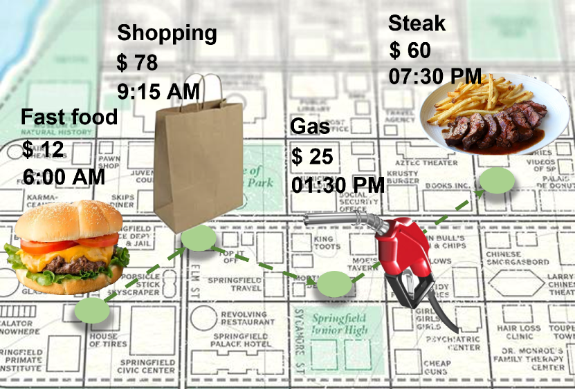
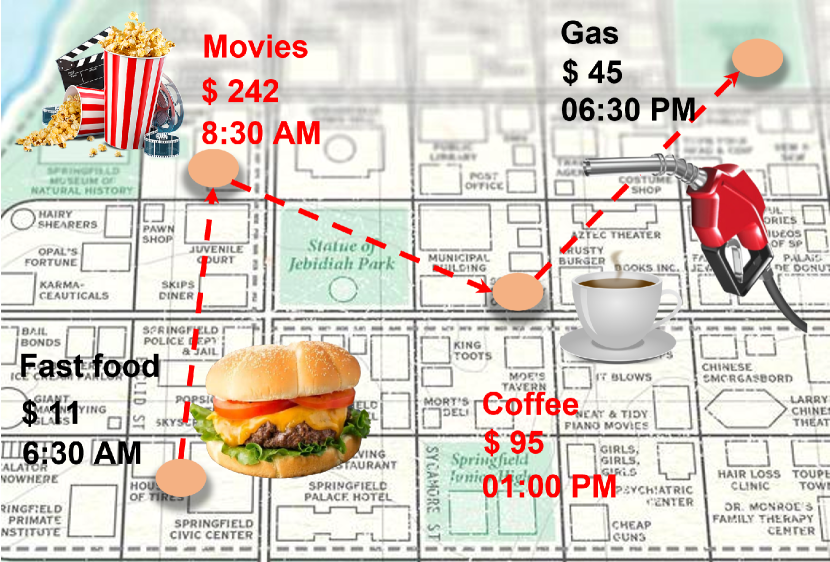
Figure 1: Examples of a sequence of ordinary events (left) and a sequence of anomalous events (right) that are dependent: one leads to another. The events on the left show an ordinary pattern of transactions for a consumer. For the events on the right, it is unusual for a consumer to execute a transaction at a movie theater in the early morning and then a high-volume transaction at a coffee shop. It indicates the events are abnormal.

For applications such as financial fraud detection, we usually only have access to the anomalous event sequences. This can be due to protecting consumer privacy, so only fraudulent transaction data are collected for the study. The resulting one-class problem makes the task of anomaly detection even more challenging. Still, there are distinctive patterns of anomalies that enable us to develop powerful detection algorithms. For instance, Figure 2(a) shows an example of a sequence of fraudulent transactions that we extracted from real data. A fraudster used a stolen card twelve times in just six days and made electronic transactions at stores that are physically far away from each other, ranging from California to New England. The types of transactions are also different from the regular spending pattern. Figure 2(b) illustrates the distribution of a collection of fraudulent transactions for location (store ID), season, and the number of transactions. We can observe a significant portion of transactions at the department store in San Francisco and New York.

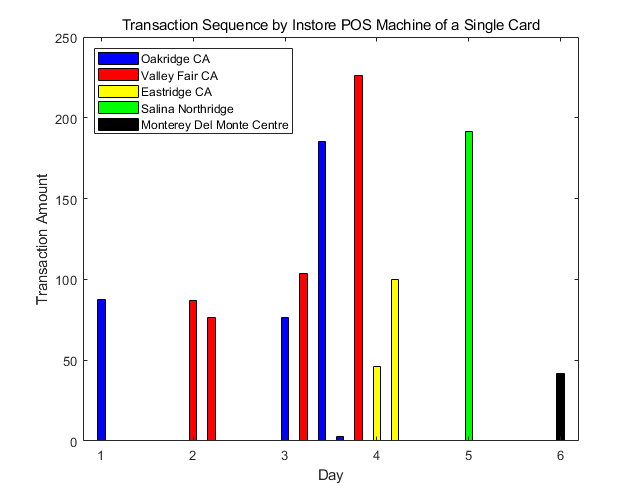
(a) transactions by one card

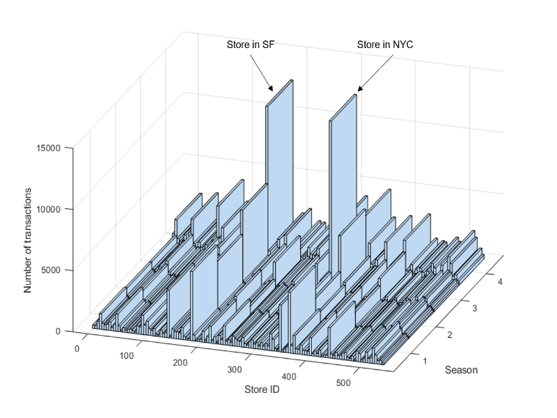
(b) locations of the transactions

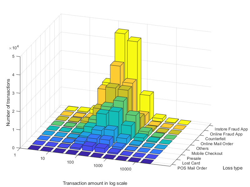
(c) types of the transactions

Figure 2: Example of sequential fraud credit card transactions data set provided by a major department store in the US: (a) shows a sequence of transactions made by one stolen credit card; each bar represents a fraudulent transaction, and the bar’s height indicates the transaction amount in dollars and the color of the bar indicates the location of the transaction; (b) shows an overview of how these fraudulent transactions were distributed over stores and seasons; (c) shows an overview of how these fraudulent transactions were distributed over the amount of purchase for different loss types.

Although there has been much research effort in machine learning and statistics for anomaly detection using sequential data [7, 55, 8, 11], we cannot use existing methods here directly for the following reasons. First, many existing works consider detecting anomalous sequences “as a whole” rather than detecting in an online fashion. Second, the one-class data situation requires an unsupervised approach for anomaly detection; however, most sequential anomaly detection algorithms are based on supervised learning.

This paper presents an adversarial anomaly detection algorithm for one-class sequential detection, where only anomalous data are available. The adversarial sequential detector is solved from a minimax problem to find an optimal detector against the worst-case sequences from a generator that captures the dependence in sequential events using the marked point process model. The detector sequentially evaluates the likelihood of a test sequence and compares it with a time-varying threshold, which is also learned from data through the minimax problem. We demonstrate the proposed method’s good performance by comparing state-of-the-art methods on synthetic and proprietary large-scale credit card fraud data provided by a major department store in the US.

On a high-level, our minimax formulation is inspired by imitation learning [21], which minimizes the maximum mean discrepancy [18] (MMD). In particular, the generator is built upon the Long Short-Term Memory (LSTM) [20] which specifies the conditional distribution of the next event. We parameterize the detector by comparing the likelihood function of marked Hawkes processes with a deep Fourier kernel [63, 58] with a threshold. The resulted likelihood function is computationally efficient to implement in the online fashion and can capture complex dependence between events in anomalous sequences. A notable feature of our framework is a time-varying threshold learned from data by solving the minimax problem, which achieves tight control of the false-alarms and hard to obtain precisely in theory. This is a drastic departure from prior approaches in sequential anomaly detection.

The rest of the paper is organized as follows. We first discuss the related work in sequential anomaly detection and revisit some basic definitions in imitation learning. Section 3 sets up the problem and introduces our sequential anomaly detection framework. Section 4 proposes a new marked point process model equipped with a deep Fourier kernel to model-dependent sequential data. Section 5 presents the adversarial sequence generator and learning algorithms. Finally, we present our numerical results on both real and synthetic data in Section 6. Proofs to all propositions can be found in the appendix.

1.1 Related work

Several research lines are related to this work, including imitation learning, the long-term-short-term (LSTM) architecture for modeling sequence data, one-class anomaly detection, and fraud detection, which we review below.

Imitation learning [21] aims to mimic the expert’s behavior in a given task. An agent (a learning machine) is trained to perform a task from demonstrations by learning a mapping between observations and actions. Landmark works by [1, 47] attack this problem via inverse reinforcement learning (IRL). In their work, the learning process is achieved by devising a game-playing procedure involving two opponents in a zero-sum game. This alteration not only allows them to achieve the same goal of doing nearly as well as the expert as in [1] but achieves better performances in various settings. However, this strategy cannot be directly applied to event data modeling without adaptation. A recent work [26] filled this gap by introducing a reward function with a non-parametric form, which measures the discrepancy between the training and generated sequences. Their proposed approach models the events using a temporal point process, which draws similarities in our work’s spatio-temporal point process model. However, our work differs from [26] in two major ways. Rather than constructing a generative model, we focus on sequential anomaly detection, which is a different type of problem. Besides, we design a structured reward function that is more suitable for modeling the triggering effects between events and more computationally efficient to carry out.

There is another work on inverse reinforcement learning related to our work. The work in [64] first proposed a probabilistic approach to the imitation learning problem via maximum entropy. The work proposed an efficient state frequency algorithm that is composed of both backward and forward passes recursively. A more recent similar article by [37] seeks to integrate IRL with anomaly detection based on the above maximum entropy IRL framework. They aim to learn the unknown reward function to test a given sequence. The significant difference, however, is they focus on time series data instead of event data. Also, we formulate the problem as a minimax optimization, whereas they used a Bayesian method to estimate the model parameters.

A large body of recent works performs sequential anomaly detection using LSTM, similar to the proposed stochastic LSTM used as the adversarial generator in our work. In [30], the authors proposed an encoder-decoder scheme using LSTM to learn the normal behavior of data and used reconstruction errors to find anomalies. The work of [35] built a Recurrent Neural Network (RNN) model with LSTM structure to conduct anomaly detection for multivariate time series data for flight operations. Another paper from [28] looks into anomaly detection in videos by convolutional neural networks with the LSTM modeling. It is clear that the LSTM model is versatile for various applications and can model unknown complex sequential data. However, the LSTM used here in this paper is stochastic (as a generative model to capture data distribution), whereas most LSTM architectures are deterministic. Specifically, the input at each time step in the stochastic LSTM is drawn from a random variable whose distribution is specified by the LSTM’s parameters.

There is a wide array of existing research in anomaly detection. Principle Component Analysis (PCA) has traditionally been used to detect outliers, which naturally fits into anomaly detection. In [5] the authors propose a robust auto-encoder model, which is closely related to PCA for anomaly detection, and a deep neural network is introduced for the training process. Additionally, [6] proposed a one-class neural network to detect anomalies in complex data sets by creating a tight envelope around the normal data. It is improved from the one-class singular value decomposition formulation to be more robust. A closely related work is [43], which looks into one-class anomaly detection through a deep support vector data description model that finds a data-enclosing hyper-sphere with minimum volume. However, most previous studies on one-class anomaly detection assumed independent and identically distributed data samples, whereas we consider data dependency.

As an important application of anomaly detection, credit card fraud detection has also drawn a lot of research interest [3, 22]. Most commonly, supervised methods have been adopted to use a database of known fraudulent/legitimate cases to construct a model that yields a suspicion score for new cases. Traditional statistical classification methods, such as linear discriminant analysis [52], logistic classification [44], and $k$-nearest neighbors [31], have proved to be effective tools for many applications. However, more powerful tools [15, 29], especially neural networks, have also been extensively applied. Unsupervised methods are used when there are no prior sets of legitimate and fraudulent observations. A large body of approaches [2, 46, 49] employed here are usually a combination of profiling and outlier detection methods, which models a baseline distribution to represent the normal behavior and then detect observations departure from this. Compared to the previous unsupervised studies in credit card fraud detection, the most notable feature of our approach is to learn the fraudulent behaviors by “mimicking” the limited amount of anomalies via an adversarial learning framework. Our anomaly detector equipped with the deep Fourier kernel is more flexible than conventional approaches in capturing intricate marked spatio-temporal dynamics between events while being computationally efficient.

Our work is a significant extension of the previous conference paper [62], which studies the one-class sequential anomaly detection using a framework of Generative Adversarial Network (GAN) [16, 17] based on the cross-entropy between the real and generated distributions. Here, we focus on a different loss function motivated by imitation learning and MMD distances that is more computationally efficient. In addition, we introduce a new time-varying threshold, which can be learned in a data-driven manner.

2 Background: Inverse reinforcement learning

Since imitation learning is a form of reinforcement learning (RL), in the following, we will provide some necessary background about RL. Consider an agent interacting with the environment. At each step, the agent selects an action based on its current state, to which the environment responds with a reward value and the next state. The return is the sum of (discounted) rewards through the agent’s trajectory of interactions with the environment. The value function of a policy describes the expected return from taking action from a state. The inverse reinforcement learning (IRL) aims to find a reward function from the expert demonstrations explaining the expert behavior. Seminal works [1, 36] provide a max-min formulation to address the problem. The authors propose a strategy to match an observed expert policy’s value function and a learner’s behavior. Let $\pi$ denote the expert policy, and $\pi_{\varphi}$ denote the learner policy, respectively. The optimal reward function $r$ can be found as the saddle-point of the following max-min problem [47], i.e.,

$$\underset{r\in\mathcal{F}}{\max}~{}\underset{\varphi\in\mathcal{G}}{\min}~{}\Bigg{\{} \mathbb{E}_{\boldsymbol{x}\sim\pi}\left[\sum_{i=1}^{N_{x}}r(x_{i},s_{i})\right]-\mathbb{E}_{\boldsymbol{z}\sim\pi_{\varphi}}\left[\sum_{j=1}^{N_{z}}r(z_{j},s_{j})\right]\Bigg{\}},$$

where $\mathcal{F}$ is the family class for reward function and $\mathcal{G}$ is the family class for learner policy. Here, $\boldsymbol{x}=\{x_{1},\dots,x_{N_{x}}\}$ is a sequence of actions generated by the expert policy $\pi$, $\boldsymbol{z}=\{z_{1},\dots,z_{N_{z}}\}$ is a roll-out sequence generated from the learner policy $\pi_{\varphi}$, and $N_{x}$ and $N_{z}$ are the numbers of actions for sequences $\boldsymbol{x}$ and $\boldsymbol{z}$, respectively. The formulation means that a proper reward function should provide the expert policy a higher reward than any other learner policy in $\mathcal{G}$. The learner can also approach the expert performance by maximizing this reward.

3 Adversarial sequential anomaly detection

We aim to develop an algorithm to detect anomalous sequences when the training dataset consists of only abnormal sequences and without normal sequences. In particular, the algorithm will process data sequentially and raise the alarm as soon as possible after the sequence has been identified as anomalous. Denote such a detector as $\ell$ with parameter $\theta$. At each time $t$, the detector evaluates a statistic and compares it with a threshold. For a length-$N$ sequence $\boldsymbol{x}$, define $\boldsymbol{x}_{1:i}:=[x_{1},\ldots,x_{i}]^{\top}$, $i=1,2,\ldots,N$ be its first $i$ observations. We define the detector as a stopping rule, which stops and raises the alarm the first time that the detection statistic exceeds the threshold:

$$T=\inf\{t:\ell(\boldsymbol{x}_{1:i};\theta)>\eta_{i},~{}t_{i}\leq t<t_{i+1}\},\quad i=1,\ldots,N.$$

Once an alarm is raised, the sequence is flagged as an anomaly. If there is no alarm raised till the end of the time horizon, the sequence is considered normal. Note that the test sequence can be an arbitrary (finite) length.

3.1 Proposed: Adversarial anomaly detection

Assume a set of anomalous sequences drawn from an empirical distribution $\pi$. Since normal sequences are not available, we introduce an adversarial generator, which produces “normal” sequences that are statistically similar to the real anomalous sequences. The detector has to discriminate the true anomalous sequence from the counterfeit “normal” sequences. We introduce competition between the anomaly detector and the generator to drive both models to improve their performances until anomalies can distinguish from the worst-case counterfeits. We can also view this approach as finding the “worst-case” distribution that defines the “border region” for detection. Formally, we formulate this as a minimax problem as follows:

$$\underset{\varphi\in\mathcal{G}}{\min}~{}\underset{\theta\in\Theta}{\max}~{}J(\theta,\varphi)\coloneqq\mathbb{E}_{\boldsymbol{x}\sim\pi}~{}\ell(\boldsymbol{x};\theta)-\mathbb{E}_{\boldsymbol{z}\sim G_{z}(\varphi)}~{}\ell(\boldsymbol{z};\theta),$$ (1)

where $G_{z}$ is an adversarial generator specified by the parameter $\varphi\in\mathcal{G}$ and $\mathcal{G}$ is a family of candidate generators. Here the detection statistic corresponds to $\ell(\theta)$, the log-likelihood function of the sequence specified by $\theta\in\Theta$ and $\Theta$ is its parameter space. The choices of the adversarial generator and the detector are further discussed in Section 4. The detector compares the detection statistic to a threshold. We define the following:

Definition 1 (Adversarial sequential anomaly detector).

Denote the solution to the minimax problem (1) as $(\theta^{*},\varphi^{*})$. A sequential adversarial detector raises an alarm at the time $i$ if

$$\ell(\boldsymbol{x}_{1:i};\theta^{*})>\eta_{i}^{*},$$

where the time-varying threshold $\eta_{i}^{*}\propto\mathbb{E}_{\boldsymbol{z}\sim G_{z}(\varphi^{*})}~{}\ell(\boldsymbol{z}_{1:i};\theta^{*})$.

3.2 Time-varying threshold

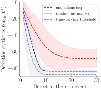
Figure 3: An example of the adversarial anomaly detection and threshold using synthetic data with 1000 synthetic sequences. The two lighter dashed lines represent mean detection statistics ($\ell(\theta^{*})$) for anomalous and normal sequences. The dashed line in the middle corresponds to the time-varying threshold suggested by our model. Clearly, the threshold can separate the anomalous sequences from the normal sequences.

We choose the time-varying threshold $\eta_{i}^{*}\propto\mathbb{E}_{\boldsymbol{z}\sim G_{z}(\varphi^{*})}~{}\ell(\boldsymbol{z}_{1:i};\theta^{*})$. Since the value of log-likelihood function $\ell(x_{1:i};\theta^{*})$ for partial sequence observation $\boldsymbol{x}_{1:i}$ may vary over the time step $i$ (the $i$-the event is occurred), we need to adjust the threshold accordingly for making decisions as a function of $i$. Note that our time-varying threshold $\eta_{i}^{*}$ is different from sequential statistical analysis, where the threshold for performing detection is usually constant or pre-set (not adaptive to data) based on the known distributions of the data sequence (e.g., set the threshold growing over time as $\sqrt{t}$ [45]). The rationale behind the design of the threshold $\eta_{i}^{*}$ is that, at any given time step, the log-likelihood of the data sequence is larger than that of the generated adversarial sequence; therefore, $\eta_{i}^{*}$ provides the tight lower bound for the likelihood of anomalous sequences $\ell(\boldsymbol{x};\theta^{*})$ due to the minimization in (1). That is, for any $\varphi\in\mathcal{G}$,

$$0\leq ~{}\mathbb{E}_{\boldsymbol{x}\sim\pi}~{}\ell(\boldsymbol{x}_{1:i};\theta^{*})-\eta_{i}^{*}$$

$$\leq ~{}\mathbb{E}_{\boldsymbol{x}\sim\pi}~{}\ell(\boldsymbol{x}_{1:i};\theta^{*})-\mathbb{E}_{\boldsymbol{z}\sim G_{z}(\varphi)}~{}\ell(\boldsymbol{z}_{1:i};\theta^{*}).$$

The adversarial sequences drawn from $G_{z}(\varphi^{*})$ can be viewed as the normal sequences that are statistically “closest” to anomalous sequences. Therefore, the log-likelihood of such sequences in the “worst-case” scenario defines the “border region” for detection. In practice, the threshold $\eta_{i}^{*}$ can be estimated by $1/n^{\prime}\sum_{l=1}^{n^{\prime}}\ell(\boldsymbol{z}^{l}_{1:i};\theta^{*})$, where $\{\boldsymbol{z}^{l}\}_{l=1,\dots,n^{\prime}}$ are adversarial sequences sampled from $G_{z}(\varphi)$ and $n^{\prime}$ is the number of the sequences. As a real example presented in Figure 3, the time-varying threshold in the darker dashed line can sharply separate the anomalous sequences from the normal sequences. More experimental results are presented in Section 6.

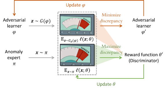
Figure 4: An illustration of the imitation learning interpretation.

3.3 Connection to imitation learning

The problem formulation (1) resembles the minimax formulation in inverse reinforcement learning (IRL) proposed by seminal works [1, 36]. As shown in Figure 4, an observed anomalous samples $\boldsymbol{x}\sim\pi$ can be regarded as an expert demonstration sampled from the expert policy $\pi$, where each $\boldsymbol{x}=\{x_{1},\dots,x_{N}\}$ is a sequence of events with length of $N$ and the sequences may be of different lengths. Each event $x_{i},i=1,\dots,N$ of the sequence is analogous to the $i$-th action made by the expert given the history of past events $\{x_{1},x_{2},\dots,x_{i-1}\}$ as the corresponding state. Accordingly, the generator can be regarded as a learner that generates convincing counterfeit trajectories.

The log-likelihood of observed sequences can be interpreted as undiscounted return, i.e., the accumulated sum of rewards evaluated at past actions, where the logarithm of the conditional probability of each event (action) can be regarded as the event’s reward. The ultimate goal of the proposed framework (1) is to close the gap between the return of the expert demonstrations and the return of the learner trajectories so that the counterfeit trajectories can meet the lower bound of the real demonstrations.

3.4 Connection to MMD-like distance

The proposed approach can also be viewed as minimizing a maximum mean discrepancy (MMD)-like distance metric [18] as illustrated in Figure 5. More specifically, the maximization in (1) is analogous to an MMD metric in a reduced function class specified by $\Theta$, i.e., $\sup_{\theta\in\Theta}~{}\mathbb{E}_{\boldsymbol{x}\sim\pi}~{}\ell(\boldsymbol{x};\theta)-\mathbb{E}_{\boldsymbol{z}\sim\varphi}~{}\ell(\boldsymbol{z};\theta)$, where $\Theta$ may not necessarily be a space of continuous, bounded functions on sample space. As shown in [18], if $\Theta$ is sufficiently expressive (universal), e.g., the function class on reproducing kernel Hilbert space (RKHS), then maximization over such $\Theta$ is equivalent to the original definition. Based on this, we select a function class that serves our purpose for anomaly detection (characterizing the sequence’s log-likelihood function), which has enough expressive power for our purposes. Therefore, the problem defined in (1) can be regarded as minimizing such an MMD-like metric between the empirical distribution of anomalous sequences and the distribution of adversarial sequences. The minimal MMD distance corresponds to the best “detection radius” that we can find without observing normal sequences.

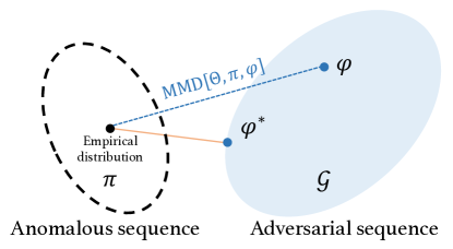
Figure 5: The empirical distribution of anomalous sequences is $\pi$. The assumed family of candidate generators is $\mathcal{G}$. Our proposed framework aims to minimize the maximum mean discrepancy (MMD) in a reduced function class $\Theta$ between $\pi$ and $\varphi\in\mathcal{G}$.

4 Point process with deep Fourier kernels

In this section, we present a model for the discrete events, which will lead to the detection statistic (i.e., the form of the likelihood function $\ell(\boldsymbol{x};\theta)$). We present a marked Hawkes process model that captures marked spatio-temporal dynamics between events. The most salient feature of the model is that we develop a novel deep Fourier kernel for Hawkes process (c.f. Section 6.6 [34] for discussion of Fourier kernel), where the deep Fourier kernel empowers the model to characterize the intricate non-linear dependence between events while enabling efficient computation of the likelihood function by leading to a closed-form expression of an integral in the likelihood function – a notorious difficulty in evaluating the likelihood function for Hawkes processes.

Assume each observation is a marked spatio-temporal tuple which consists of time, location, and marks: $x_{i}=(t_{i},m_{i})$, where $t_{i}\in[0,T)$ is the time of occurrence of the $i$th event, and $m_{i}\in\mathcal{M}\subseteq\mathbb{R}^{d}$ is the $d$-dimensional mark (here we treat location as one of a mark). The event’s time is important because it defines the event’s order and the time interval, which carries the key information.

4.1 Preliminary: Marked temporal point processes

The marked temporal point processes (MTPPs) [19, 41] offer a versatile mathematical framework for modeling sequential data consisting of an ordered sequence of discrete events localized in time and mark spaces (space or other additional information). They have proven useful in a wide range of applications [13, 9, 27, 40, 25]. Recent works [12, 32, 26, 50, 54, 53, 62] have achieved many successes in modeling temporal event data (some with marks) correlated in the time domain using Recurrent Neural Networks (RNNs).

Let $\{x_{1},x_{2},\dots,x_{N_{T}}\}$ represent a sequence of observations. Denote $N_{T}$ as the number of the points generated in the time horizon $[0,T)$. The events’ distributions in MTPPs are characterized via a conditional intensity function $\lambda(t,m|\mathcal{H}_{t})$, which is the probability of observing an event in the marked temporal space $[0,T)\times\mathcal{M}$ given the events’ history $\mathcal{H}_{t}=\{(t_{i},m_{i})|t_{i}<t\}$, i.e.,

$$\lambda(t,m|\mathcal{H}_{t})=\frac{\mathbb{E}\left[N([t,t+dt)\times B(m,dm))|\mathcal{H}_{t}\right]}{|B(m,dm)|dt},$$ (2)

where $N(A)$ is the counting measure of events over the set $A\subseteq[0,T)\times\mathcal{M}$ and $|B(m,dm)|$ is the Lebesgue measure of the ball $B(m,dm)$ centered at $m$ with radius $dm$. Assuming that influence from past events are linearly additive for the current event, the conditional intensity function of a Hawkes process is defined as

$$\lambda(t,m|\mathcal{H}_{t})=\mu+\sum_{t_{i}<t}g(t-t_{i},m-m_{i}),$$ (3)

where $\mu\geq 0$ is the background intensity of events, $g(\cdot,\cdot)\geq 0$ is the triggering function that captures spatio-temporal and marked dependencies of the past events. The triggering function can be chosen in advance, e.g., in one-dimensional cases, $g(t-t_{i})=\alpha\exp\{-\beta(t-t_{i})\}$.

Let $t_{n}$ denote the last occurred event before time $t$. The conditional probability density function of a point process is defined as

$$f(t,m|\mathcal{H}_{t})=\lambda(t,m|\mathcal{H}_{t})\exp\left\{-\int_{t_{n}}^{t}\int_{\mathcal{M}}\lambda(t^{\prime},m^{\prime}|\mathcal{H}_{t^{\prime}})dm^{\prime}dt^{\prime}\right\}.$$

The log-likelihood of observing a sequence with $N_{T}$ events denoted as $\boldsymbol{x}=\{(t_{i},m_{i})\}_{i=1}^{N_{T}}$ can be obtained by:

$$\ell(\boldsymbol{x};\theta)=\sum_{i=1}^{N_{T}}\log\lambda(t_{i},m_{i}|\mathcal{H}_{t_{i}})-\int_{0}^{T}\int_{\mathcal{M}}\lambda(t,m|\mathcal{H}_{t})dmdt.$$ (4)

4.2 Hawkes processes with deep Fourier kernel

One major computational challenge in evaluating the log-likelihood function is the computation of the integral in (4), which is multi-dimensional and performed in the possibly continuous mark and time-space. It can be intractable for a general model without a carefully crafted structure.

To tackle this challenge, we adopt an approach to represent the Hawkes process’s triggering function via a Fourier kernel. The Fourier features spectrum is parameterized by a deep neural network, as shown in Figure 6. For the sake of notational simplicity, we denote $x\coloneqq(t,m)\in\mathcal{X}$ as the most recent event and $x^{\prime}\coloneqq(t^{\prime},m^{\prime})\in\mathcal{X},~{}t^{\prime}<t$ as an occurred event in the past, where $\mathcal{X}\coloneqq[0,T]\times\mathcal{M}\subset\mathbb{R}^{d+1}$ is the space for time and mark. Define the conditional intensity function as

$$\lambda(x|\mathcal{H}_{t};\theta)=\mu+\alpha\sum_{t^{\prime}<t}K(x,x^{\prime}),$$ (5)

where $\alpha$ represents the magnitude of the influence from the past, $\mu\geq 0$ is the background intensity of events. The kernel function $K(x,x^{\prime})$ measures the influence of the past event on the current event $x,x^{\prime}\in\mathcal{X}$, and we will parameterize its kernel-induced feature mapping using a deep neural network $\theta\in\Theta$.

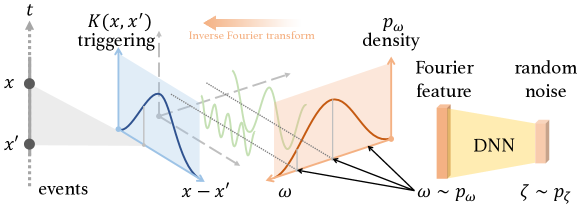
Figure 6: An illustration of the Fourier kernel function $K(x,x^{\prime})$ and its Fourier representation; a deep neural network represents the spectrum of Fourier features.

The formulation of deep Fourier kernel function relies on Bochner’s Theorem [42], which states that any bounded, continuous, and shift-invariant kernel is a Fourier transform of a bounded non-negative measure:

Theorem 1 (Bochner [42]).

A continuous kernel of the form $K(x,x^{\prime})=g(x-x^{\prime})$ defined over a locally compact set $\mathcal{X}$ is positive definite if and only if $g$ is the Fourier transform of a non-negative measure:

$$K(x,x^{\prime})=g(x-x^{\prime})=\int_{\Omega}p_{\omega}(\omega)e^{\boldsymbol{i}w^{\top}(x-x^{\prime})}d\omega,$$ (6)

where $\boldsymbol{i}=\sqrt{-1}$, $p_{\omega}$ is a non-negative measure, $\Omega$ is the Fourier feature space, and kernels of the form $K(x,x^{\prime})$ are called shift-invariant kernel.

If a shift-invariant kernel in (6) is positive semi-definite and scaled such that $g(0)=1$, Bochner’s theorem ensures that its Fourier transform $p_{\omega}$ can be viewed as a probability distribution function since it normalize to 1 and is non-negative. In this sense, the spectrum $p_{\omega}$ can be viewed as the distribution of $r$-dimensional Fourier features indexed by $\omega\in\Omega\subset\mathbb{R}^{r}$. Hence, we may obtain a triggering function in (5) between two events $x,x^{\prime}\in\mathcal{X}\subset\mathbb{R}^{d+1}$ which satisfies the “kernel embedding”:

Proposition 1.

Let the triggering function $K$ be a continuous real-valued shift-invariant kernel and $p_{\omega}$ a probability distribution function. Then

$$K(x,x^{\prime})\coloneqq\mathbb{E}_{\omega\sim p_{\omega}}\big{[}\phi_{\omega}(x)\cdot\phi_{\omega}(x^{\prime})\big{]},$$ (7)

where $\phi_{\omega}(x)\coloneqq\sqrt{2}\cos(\omega^{\top}Wx+u)$ and $W\in\mathbb{R}^{r\times(d+1)}$ is a weight matrix. These Fourier features $\omega\in\Omega\subset\mathbb{R}^{r}$ are sampled from $p_{\omega}$ and $u$ is drawn uniformly from $[0,2\pi]$.

In practice, the expression (7) can be approximated empirically, i.e.,

$$\widetilde{K}(x,x^{\prime})=\frac{1}{D}\sum_{k=1}^{D}\phi_{\omega_{k}}(x)\cdot\phi_{\omega_{k}}(x^{\prime})=\Phi(x)^{\top}\Phi(x^{\prime}),$$ (8)

where $\omega_{k},~{}k=1,\dots,D$ are $D$ Fourier features sampled from the distribution $p_{\omega}$. The vector $\Phi(x)\coloneqq[\phi_{\omega_{1}}(x),\dots,\phi_{\omega_{D}}(x)]^{\top}$ can be viewed as the approximation of the kernel-induced feature mapping for the score. In the experiments, we substitute $\exp\{\boldsymbol{i}w^{\top}(x-x^{\prime})\}$ with a real-valued feature mapping, such that the probability distribution $p_{\omega}$ and the kernel $K$ are real [39].

The next proposition shows the empirical estimation (8) converges to the population value uniformly over all points in a compact domain $\mathcal{X}$ as the sample size $D$ grows. It is a lower variance approximation to (7).

Proposition 2.

Assume $\sigma_{p}^{2}=\mathbb{E}_{\omega\sim p_{\omega}}[\omega^{\top}\omega]<\infty$ and a compact set $\mathcal{X}\subset\mathbb{R}^{d+1}$. Let $R$ denote the radius of the Euclidean ball containing $\mathcal{X}$. Then for the kernel-induced feature mapping $\Phi$ defined in (8), we have

$$\mathbb{P}\left\{\underset{x,x^{\prime}\in\mathcal{X}}{\sup}\left|\Phi(x)^{\top}\Phi(x^{\prime})-K(x,x^{\prime})\right|\geq\epsilon\right\}\leq~{}\left(\frac{48R\sigma_{p}}{\epsilon}\right)^{2}\exp\left\{-\frac{D\epsilon^{2}}{4(d+3)}\right\}.$$ (9)

The proposition ensures that kernel function can be consistently estimated using a finite number of Fourier features. In particular, note that for an error bound $\epsilon$, the number of samples needed is on the order of $D=O((d+1)\log(R\sigma_{p}/\epsilon)/\epsilon^{2})$, which grows linearly as data dimension $d$ increases, implying the sample complexity is mild in the high-dimensional setting.

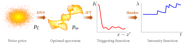
Figure 7: An instance of calculating the conditional intensity $\lambda$ through performing inverse Fourier transform: (1) generate random noise; (2) map the noises to the frequencies according to the optimal spectrum; (3) performs inverse Fourier transform (IFT) in the frequency domain and obtain the triggering function; (4) calculate the intensity function based on the triggering function.

To represent the distribution $p_{\omega}$, we assume it is a transformation of random noise $\zeta\sim p_{\zeta}$ through a non-linear mapping $\psi_{0}:\mathbb{R}^{q}\rightarrow\mathbb{R}^{r}$, as shown in Figure 6, where $\psi_{0}$ is a differentiable and it is represented by a deep neural network and $q$ is the dimension of the noise. Roughly speaking, $p_{\omega}$ is the probability density function of $\psi_{0}(\zeta)$, $\zeta\sim p_{\zeta}$. Note that the triggering kernel is jointly controlled by the deep network parameters and the weight matrix $W$. We represent the Fourier feature generator as $G_{\zeta}$ and denote its parameters as $\theta\in\Theta$.

Figure 7 gives an illustrative example of representing the conditional intensity given sequence history using our approach. We choose $q=r=2$ to visualize the noise prior $p_{\zeta}$ and the optimal spectra $p^{*}_{\omega}$ in a two-dimensional space. The optimal spectrum learned from data uniquely specifies a kernel function capable of capturing various non-linear triggering effects. Unlike Hawkes processes, underlying long-term influences of some events, in this case, can be preserved in the intensity function.

4.3 Efficient computation of log-likelihood function

As discussed in Section 4.2, the technical difficulty of evaluating the log-likelihood function is to perform the multi-dimensional integral of the kernel function. In particular, given a sequence of events $\boldsymbol{x}$, the log-likelihood function of our model can be written by substituting the conditional intensity function in (4) with (5), and thus we need to evaluate $\int_{\mathcal{X}}\lambda(x|\mathcal{H}_{t};\theta)dx$. In many existing works, this term is carried out by numerical integration, which can be computationally expensive. For instance, if we randomly sample $\kappa$ points in a $d$-dimensional space and the total number of events is $N$, the computational complexity will be $O(\kappa DN)$ ($\kappa\gg N^{d}$) using common numerical integration techniques. Here we present a way to simplify the computation by deriving a closed-form expression for the integral as presented in the following proposition – a benefit offered by the Fourier kernel.

Proposition 3 (Integral of conditional intensity function).

Let $t_{N_{T}+1}=T$ and $t_{0}=0$. Given ordered events $\{x_{1},\dots,x_{N_{T}}\}$ in the time horizon $[0,T]$. The integral term in the log-likelihood function can be written as

$$\int_{\mathcal{X}}\lambda(x|\mathcal{H}_{t};\theta)dx=\mu T(b-a)^{d}+\frac{1}{D}\sum_{k=1}^{D}\sum_{i=0}^{N_{T}}\sum_{t_{j}<t_{i}}$$ (10)

$$\cos\left(-\omega_{k}^{\top}Wx_{j}\right)\cos\left(\frac{t_{i+1}+t_{i}}{2}\right)\sin\left(\frac{t_{i+1}-t_{i}}{2}\right)\cos^{d}\left(\frac{b+a}{2}\right)\sin^{d}\left(\frac{b-a}{2}\right)\prod_{\ell=1}^{d+1}\frac{2e^{\omega_{k}^{\top}w_{\ell}}}{\omega_{k}^{\top}w_{\ell}},$$

where $w_{\ell},\ell=1,\dots,d$ is the $\ell$-th column vector in the matrix $W$, and $[a,b]$ are the range for each dimension of the mark space $\mathcal{M}$. Note that the computational complexity is $O(DN)$.

Remark 1.

From the right-hand side of (10), the second term only depends on the weight matrix $W$, $D$ randomly sampled Fourier features, the time of events that occurred before $t$, and the region of the marked space. If we re-scale the range of each coordinate of the mark to be $[0,2\pi]$, i.e., $b=2\pi$ and $a=0$, then the second term of the integral equals to 0 and the integral defined in (10) can be further simplified as

$$\int_{\mathcal{X}}\lambda(x|\mathcal{H}_{t};\theta)dx=\mu T(2\pi)^{d}.$$

In particular, when we only consider time ($d=0$), the integral becomes:

$$\int_{\mathcal{X}}\lambda(x|\mathcal{H}_{t};\theta)dx=\mu T+\frac{1}{D}\sum_{k=1}^{D}\sum_{i=0}^{N_{T}}\sum_{t_{j}<t_{i}}\cos\left(-\omega_{k}^{\top}Wx_{j}\right)\cos\left(\frac{t_{i+1}+t_{i}}{2}\right)\sin\left(\frac{t_{i+1}-t_{i}}{2}\right)\frac{2e^{\omega_{k}^{\top}W}}{\omega_{k}^{\top}W}.$$

4.4 Recursive computation of log-likelihood function

Note that, leveraging the conditional probability decomposition, we can compute of the log-likelihood function $\ell(\boldsymbol{x}_{1:i};\theta^{*})$ recursively:

$$\ell(\boldsymbol{x}_{1:1};\theta^{*})= ~{}\log f(x_{1}|\mathcal{H}_{t_{1}});$$ (11)

$$\ell(\boldsymbol{x}_{1:i};\theta^{*})= ~{}\ell(\boldsymbol{x}_{1:i-1};\theta^{*})+\log f(x_{i}|\mathcal{H}_{t_{i}};\theta^{*}),~{}\forall i>1,$$

where

$$f(x_{i}|\mathcal{H}_{t_{i}};\theta)=\lambda(x_{i}|\mathcal{H}_{t_{i}};\theta)e^{-\mu(t_{i}-t_{i-1})(2\pi)^{d}}.$$

This recursive expression makes it convenient to evaluate the detection statistic sequentially and perform online detection, which we summarize in Algorithm 1.

Input: An unknown sequence $\boldsymbol{x}$ with $N_{T}$ events and optimal model parameters $\theta^{*},\varphi^{*}$;

Generate $D$ Fourier features from $G_{\zeta}(\theta^{*})$ denoted as $\widehat{\Omega}=\{\omega_{k}\}_{k=1,\dots,D}$;

Generate $n^{\prime}$ adversarial sequences from $G_{z}(\varphi^{*})$ denoted as $\widehat{Z}=\{\boldsymbol{z}^{l}\}_{l=1,\dots,n^{\prime}}$;

while $i\leq N_{T}$ do

       Compute the log-likelihood $\ell(\boldsymbol{x}_{1:i};\theta^{*})$ given $\widehat{\Omega}$ according to (11);

       $\eta^{*}_{i}\leftarrow 1/n^{\prime}\sum_{l=1}^{n^{\prime}}\ell(\boldsymbol{z}^{l}_{1:i};\theta^{*})$;

       if $\ell(\boldsymbol{x}_{1:i};\theta)\geq\eta_{i}^{*}$ then

             Declare that it is an anomaly and record the stopping time $t_{i}$;

            

       end if

      $i\leftarrow i+1$;

      

end while

Declare that it is not an anomaly;

Algorithm 1 Online detection algorithm

5 Adversarial sequence generator

Now we describe the parameterization for the adversarial sequence generator. To achieve rich representation power for the adversarial generator $G_{z}$, we borrow the idea of the popular Recurrent Neural Network (RNN) structure.

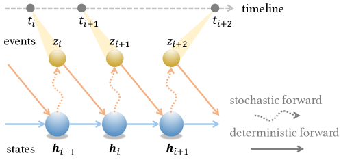
Figure 8: RNN-based adversarial sequence generator.

In particular, we develop an RNN-type generator with stochastic neurons [26, 8] as shown in Figure 8, which can represent the nonlinear and long-range sequential dependency structure. Denote the $i$-th generated adversarial event as $z_{i}\coloneqq(t_{i-1}+\Delta t_{i},m_{i})$, where $\Delta t_{i}$ is the time interval between event $z_{i-1},z_{i}$. The generating process is described below:

$$[\Delta t_{i},m_{i}^{\top}]^{\top} \sim\mathcal{N}(\boldsymbol{\mu}_{i-1},\text{diag}(\boldsymbol{\sigma}_{i-1})),$$

$$[\boldsymbol{\mu}_{i},\boldsymbol{\sigma}_{i}^{\top}]^{\top} =\psi_{1}(\boldsymbol{h}_{i}),$$

$$\boldsymbol{h}_{i} =\psi_{2}(\boldsymbol{h}_{i-1},z_{i}),~{}~{}i=1,\dots,N_{T},$$

$$\boldsymbol{h}_{0} =\boldsymbol{0},~{}$$

where the hidden state $\boldsymbol{h}_{i}\in\mathbb{R}^{p}$ encodes the sequence of past events $\{z_{1},\dots,z_{i-1}\},z_{i}\in\mathcal{X}$; $\mathcal{N}(\boldsymbol{\mu},\Sigma)$ stands for the multivariate Gaussian distribution with mean $\boldsymbol{\mu}\in\mathbb{R}^{d+1}$ and covariance matrix $\Sigma\in\mathbb{R}^{({d+1})\times({d+1})}$; here we only consider variance terms and thus the covariance matrix is diagonal with diagonal entries specified by a vector $\boldsymbol{\sigma}_{i}$, and $\mbox{diag}(\boldsymbol{x})$ means to convert the vector $\boldsymbol{x}$ to a diagonal matrix. Here we adopt the (two-sided) truncated normal distribution in our adversarial sequence generator by bounding the support of each mark to the interval $(a,b)$. The probabilistic density function (p.d.f.) therefore is given by $\mathcal{N}(x|\mu,\sigma,a,b)=(1/\sigma)\phi((x-\mu)/\sigma)/({\Phi((b-\mu)/\sigma)-\Phi((a-\mu)/\sigma})),$ where $\phi(x)$ is the p.d.f. of a standard normal distribution and $\Phi(x)$ is the corresponding cumulative density function (c.d.f.); $\mu,\sigma$ are represented by the LSTM structure, and $a,b$ are determined such that the percentage of density that lie within an interval for the normal is 99.7% (the so-called three-sigma rule-of-thumb). Note that the process stops running until $t_{i}<T$ and $t_{i}+\Delta t_{i+1}\geq T$.

Function $\psi_{2}:\mathbb{R}^{p+d+1}\rightarrow\mathbb{R}^{p}$ is an extended LSTM cell and function $\psi_{1}:\mathbb{R}^{p}\rightarrow\mathbb{R}^{(d+1)^{2}+d+1}$ can be any nonlinear mappings. There are two significant differences from the vanilla version of RNNs: (1) the outputs are sampled from hidden states rather than obtained by deterministic transformations (as in the vanilla version); randomly sampling will allow the learner to explore the events’ space; (2) the sampled time point will be fed back to the RNN. We note that the model architecture for $\psi_{1}$ may be problem-specific. For example, $\psi_{1}$ can be represented by convolution neural network (CNN) [23] if the high dimensional marks are images and can be represented by LSTM or Bidirectional Encoder Representations from Transformers (BERT) [10] if the marks are text. In this paper, because the mark is three-dimensional, we use a fully-connected neural network to represent $\psi_{1}$, which achieves significantly better performance than baselines. The set of all trainable parameters in $\psi_{1},\psi_{2}$ are denoted by $\varphi\in\mathcal{G}$.

input: dataset $X=\{\boldsymbol{x}^{i}\}_{i=1,\dots,n}$;

initialization: model parameters $\theta,\varphi$;

for $1,\dots,M_{0}$ do

       (1) Randomly draw $n^{\prime\prime}$ training sequences from $X$ denoted as $\widehat{X}=\{\boldsymbol{x}^{l}\in X\}_{l=1,\dots,n^{\prime\prime}}$;

       (2) Generate $n^{\prime}$ adversarial sequences from $G_{z}(\varphi)$ denoted as $\widehat{Z}=\{\boldsymbol{z}^{l}\}_{l=1,\dots,n^{\prime}}$;

       (3) Generate $D$ Fourier features from $G_{\zeta}(\theta)$ denoted as $\widehat{\Omega}=\{\omega_{k}\}_{k=1,\dots,D}$;

       Update $\varphi$ by descending gradient given $\widehat{X},\widehat{Z},\widehat{\Omega}$:

$$\nabla_{\varphi}\frac{1}{n^{\prime\prime}}\sum_{l=1}^{n^{\prime\prime}}\ell(\boldsymbol{x}^{l};\theta)-\frac{1}{n^{\prime}}\sum_{l=1}^{n^{\prime}}\ell(\boldsymbol{z}^{l};\theta);$$

       for $1,\dots,M_{1}$ do

             Redo steps (1), (2), (3) to obtain new $\widehat{X},\widehat{Z},\widehat{\Omega}$;

             Update $\theta$ by ascending gradient given $\widehat{X},\widehat{Z},\widehat{\Omega}$:

$$\nabla_{\theta}\frac{1}{n^{\prime\prime}}\sum_{l=1}^{n^{\prime\prime}}\ell(\boldsymbol{x}^{l};\theta)-\frac{1}{n^{\prime}}\sum_{l=1}^{n^{\prime}}\ell(\boldsymbol{z}^{l};\theta);$$

            

       end for

      

end for

Algorithm 2 Adversarial learning algorithm

We learn the adversarial detector’s parameters in an off-line fashion by performing alternating minimization between optimizing the generator $G_{z}(\varphi)$ and optimizing the anomaly discriminator $\ell(\theta)$, using stochastic gradient descent. Let $M_{0}$ be the number of iterations, and $M_{1}$ be the number of steps to apply to the discriminator. Let $n^{\prime},n^{\prime\prime}<n$ be the number of generated adversarial sequences and the number of training sequences in a mini-batch, respectively. We follow the convention of choosing mini batch size in stochastic optimization algorithm [24], and only require to use the same value for both $n^{\prime}$ and $n^{\prime\prime}$. There is a clear trade-off between the model generalization and the estimation accuracy. Large $n^{\prime}$ and $n^{\prime\prime}$ tend to converge to sharp minimizers of the training and testing functions, which lead to poorer generalization. In contrast, small $n^{\prime}$ and $n^{\prime\prime}$ consistently converge to flat minimizers due to the inherent noise in the gradient estimation. We also note that large $n^{\prime}$ and $n^{\prime\prime}$ may cause the training to be computationally expensive. The learning process is summarized in Algorithm 2.

6 Numerical experiments

In this section, comprehensive numerical studies are presented to compare the proposed adversarial anomaly detector’s performance with the state-of-the-art.

6.1 Comparison and performance metrics

We compare our method (referred to as AIL) with four state-of-the-art approaches: the one-class support vector machine [56] (One-class SVM), the cumulative sum of features extracted by principal component analysis [38] (PCA+CUMCUM), the local outlier factor [4] (LOF), and a recent work leveraging IRL framework for sequential anomaly detection [37] (IRL-AD).

The performance metrics are standard, including precision, recall, and $F_{1}$ score, all of which have been widely used in the information retrieval literature [33]. This choice is because anomaly detection can be viewed as a binary classification problem, where the detector identifies if an unknown sequence is an anomaly. The $F_{1}$ score combines the precision and recall. Define the set of all true anomalous sequences as $U$, the set of positive sequences detected by the optimal detector as $V$. Then precision $P$ and recall $R$ are defined by:

$$P=|U\cap V|/|V|,~{}R=|U\cap V|/|U|,$$

where $|\cdot|$ is the number of elements in the set. The $F_{1}$ score is defined as $F_{1}=2PR/(P+R)$ and the higher $F_{1}$ score the better. Since positive and negative samples in real data are highly unbalanced, we do not use the receiver operating characteristic (ROC) curve (true positive rate versus false-positive rate) in our setting.

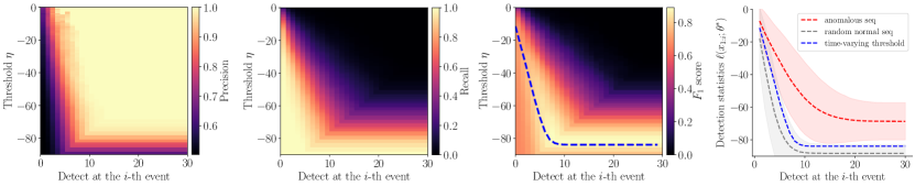
(a) singleton synthetic data

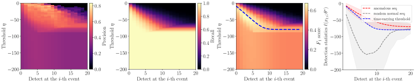
(b) composite synthetic data

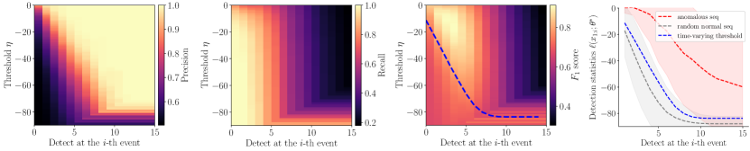
(c) real credit card fraud data

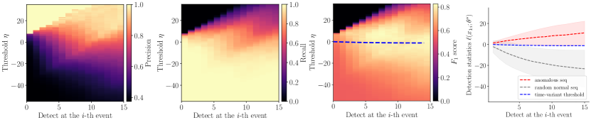
(d) real robbery data

Figure 9: The performance of our method (AIL) on four data sets. The first three columns correspond to the precision, recall, and $F_{1}$ score of our method using different thresholds. The dashed lines in the third column indicate our time-varying thresholds. The fourth column shows the step-wise detection statistics for both anomalous and normal sequences.

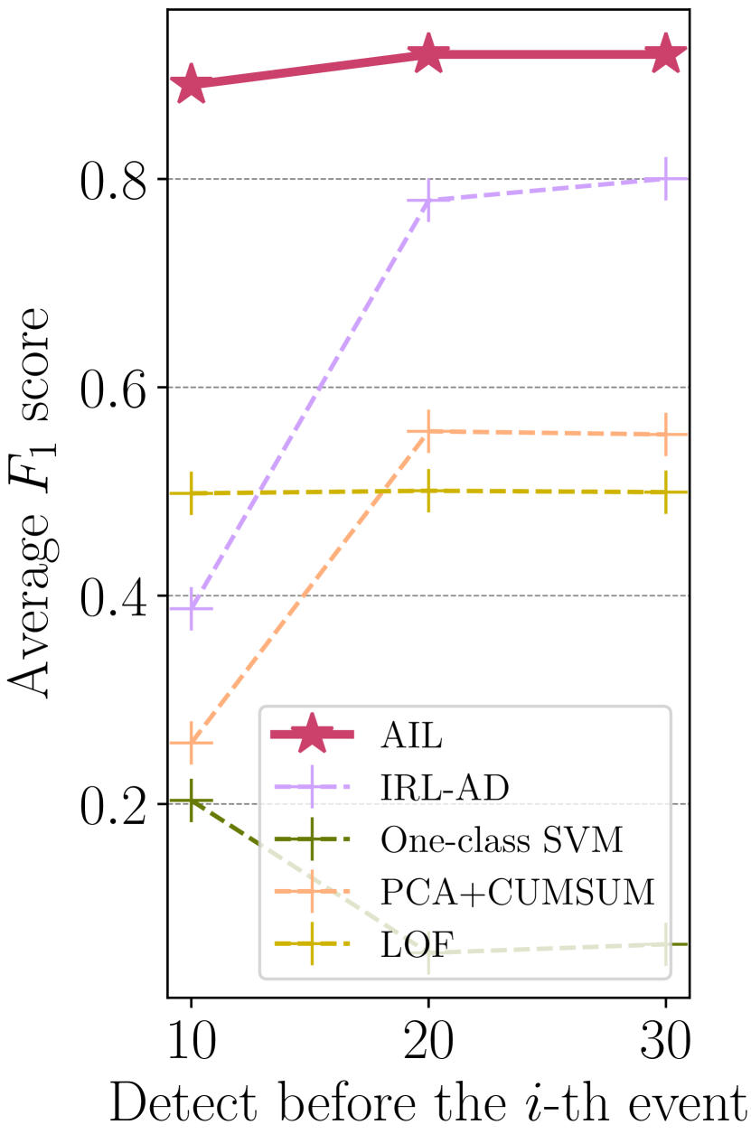
(a) singleton synthetic

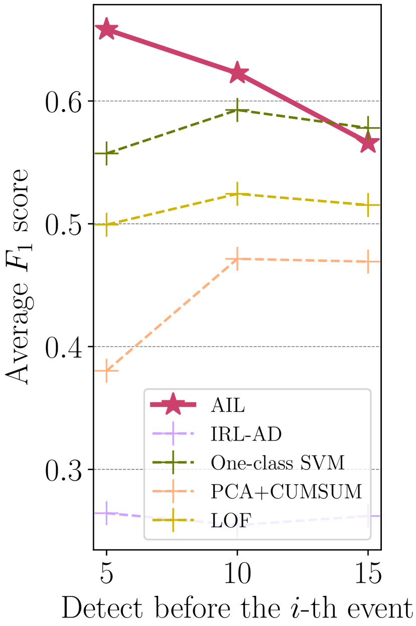
(b) composite synthetic

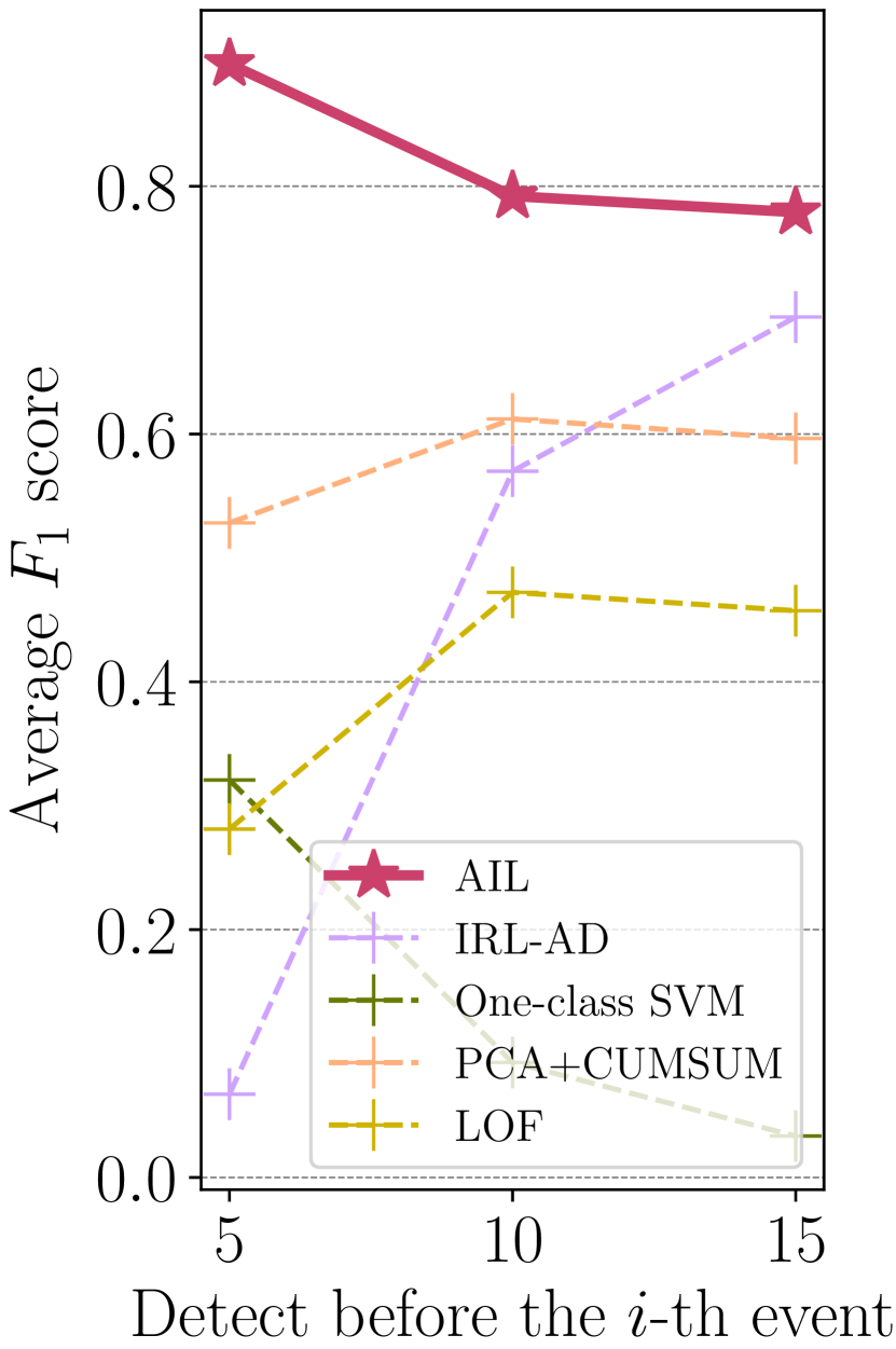
(c) credit card fraud

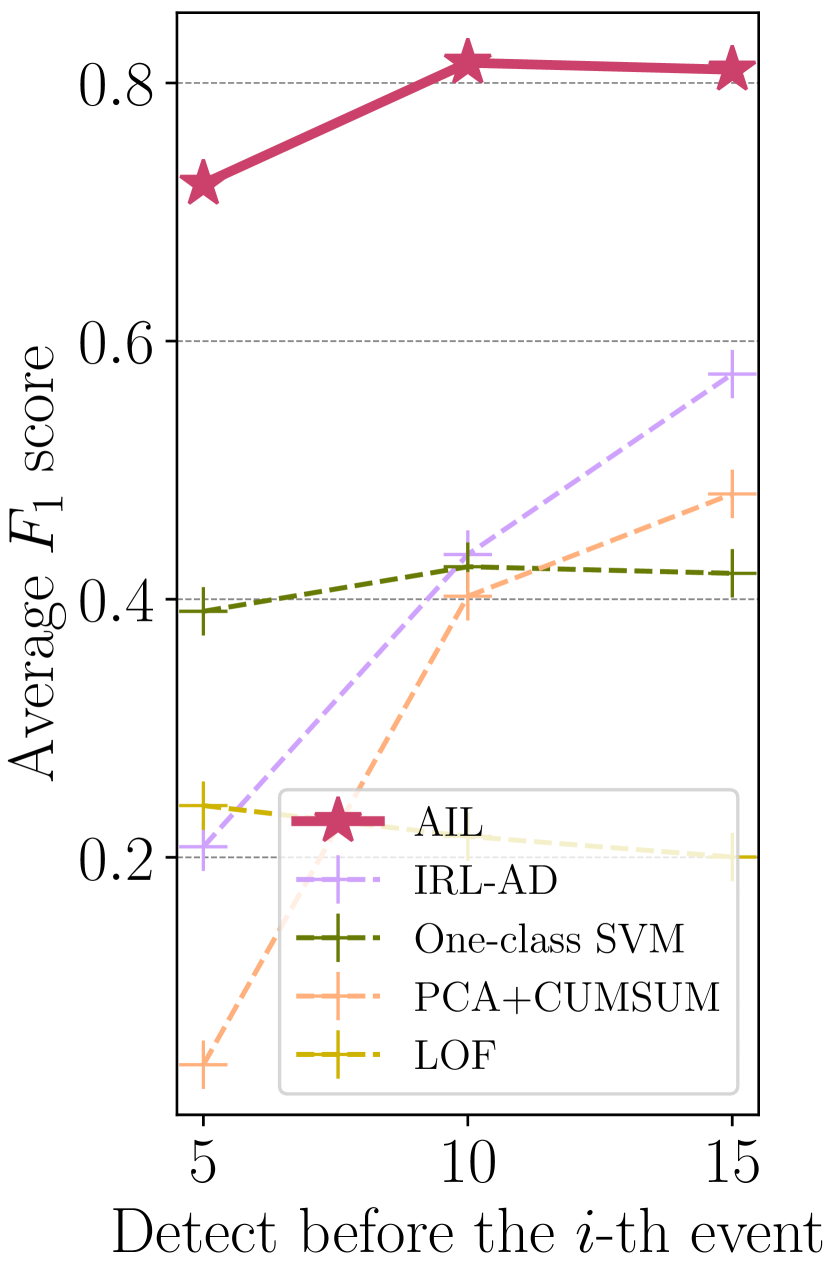
(d) robbery

Figure 10: The performance of our method (AIL) and four baselines on three data sets. The marks show the average $F_{1}$ score tested on testing sequences when decisions are made with observing part of the sequences.

6.2 Experiments set-up

Consider two synthetic and two real data sets: (1) singleton synthetic data consists of 1,000 anomalous sequences with an average length of 32. Each sequence is simulated by a Hawkes process with an exponential kernel specified in (3), where $\beta=3$ and $\mu=10,\alpha=1$; (2) composite synthetic data consists of 1,000 mixed anomalous sequences with an average length of 29. Every 200 of the sequences are simulated by five Hawkes processes with different exponential kernels, where $\mu=10,\alpha=1$, and $\beta=1,2,3,4,5$, respectively; and a real dataset (3) real credit card fraud data consists of 1,121 fraudulent credit transaction sequences with an average length of 21. Each anomalous transaction in a sequence includes the occurrence geolocation (latitude and longitude), time, and corresponding transaction amount in the dollar. (4) Robbery data contains the 911-calls-for-service events in Atlanta from 2015 to 2017 (see, e.g., [59, 60, 61, 57]). We consider each crime series as a sequence of events: each event consists of the time (in seconds) and the geolocation (in latitude and longitude), indicating when and where the event occurred. We extract a series of events in the same category identified by the police detectives and treat them as one sequence. There exists intricate spatial and temporal dependency between these events with the same category. As indicated by [61], the 911 calls of some crime incidents committed by the same individual share similar crime behaviours (e.g., forced entry) and tend to aggregate in time and space. This phenomenon is called modus operandi (M.O.) [51]. Within two years of data, this gives us 44 sequences with the sub-category of robbery. We test whether the algorithm can discriminate a series that is a robbery series or not. To create such an experiment, we also created 391 other types of crime series, which consist of randomly selected categories mixed together. We treat them as “anomalous” and “normal” data, respectively. In the experiments, we under-sample the Fourier features, where $D=20$, to improve training efficiency. In addition, we select $n^{\prime}=n^{\prime\prime}=32$ empirically based on the computational resource of the experimental set-up on a standard laptop with a quad-core 4.7 GHz processor. The model obtains its convergence around $M_{0}=1,000$ iterations with $M_{1}=5$.

Our evaluation procedure is described as follows. We consider two sets of simulation data and two sets of real data, respectively. Each data set is divided into 80% for training and 20% for testing. To evaluate the performance of the fitted model, we first mix the testing set with 5,000 normal sequences, which are simulated by multiple Poisson processes, and then perform online detection. Note that we do not simulate normal sequences for the robbery data experiment, since we treat other types of crime as the alternative. The precision, recall, and $F_{1}$ score will be recorded accordingly. The method with higher precision, recall, and $F_{1}$ score at an earlier time step is more favorable than the others.

6.3 Results

First, we summarize the performance of our method on three data sets in Figure 9 and confirm that the proposed time-varying threshold can optimally separate the anomalies from normal sequences. To be specific, the fourth column in Figure 9 shows the average log-likelihood (detection statistics) and its corresponding 1$\sigma$ region for both anomalous sequences and normal sequences. As we can see, the anomalous sequences attain a higher average log-likelihood than the normal sequences for all three data sets. Their log-likelihoods fall into different value ranges with rare overlap. Additionally, the time-varying threshold indicated by darker dash lines lies between the value ranges of anomalous and normal sequences, which produces an amicable separation of these two types of sequences at any given time. The first three columns in Figure 9 present more compelling evidence that the time-varying threshold is near-optimal. Colored cells of these heat-maps are calculated with different constant thresholds $\eta$ at each step $i$ by performing cross-validation. The brightest regions indicate the “ground truth” of the optimal choices of the threshold. As shown in the third column, the time-varying thresholds are very close to the optimal choices found by cross-validation.

Table 1: $F_{1}$ score before $i$-th event using different adversarial generators in the proposed framework.

Generator in AIL	Singleton synthetic data				Composite synthetic data
	$i=5$	$i=10$	$i=15$		$i=5$	$i=10$	$i=15$
vanilla Hawkes process	.821	.889	.911		.421	.411	.370
vanilla LSTM	.761	.830	.878		.594	.542	.519
proposed extended LSTM	.888	.916	.916		.658	.623	.566

We also compare the step-wise $F_{1}$ scores of our method with the other four baselines in Figure 10. The results show that (1) from an overall standpoint, our method outperforms other baselines with significantly higher $F_{1}$ scores and (2) our method allows for easier and faster detection of anomalous sequences (before ten events being observed in our experiments), which is critically vital in sequential scenarios for most of the applications.

Finally, we present an ablation study to investigate the performance of our method using different generators. As shown in Table 1, the proposed generator based on an extended LSTM structure significantly outperforms other generators in step-wise $F_{1}$ score. As a sanity check, the generator using the vanilla Hawkes process achieves competitive performances on the singleton synthetic data since the true anomalous sequences are from a Hawkes process; However, we can observe a dramatic performance deterioration on the composite synthetic data. The anomalous sequences are generated by multiple distributions and can hardly be captured by the vanilla Hawkes process. This result confirms that using a generic generative model cannot achieve the best performance.

7 Conclusion and Discussions

We have presented a novel unsupervised anomaly detection framework on sequential data based on adversarial learning. A robust detector can be found by solving a minimax problem, and the optimal generator also helps define the time-varying threshold for making decisions in an online fashion. We model the sequential event data using a marked point process model with a neural Fourier kernel. Using both synthetic and real data, we demonstrated that our proposed approach outperforms other state-of-the-art. In particular, the experimental results suggest that the proposed framework has achieved excellent performance on a proprietary large-scale credit-card fraud dataset from a major department store in the U.S., which shows the potential of proposed methods to apply to real-world problems.

Given the prevalence of sequential event data (in many applications, there is only one-class data), we believe our proposed method can be broadly applicable to many scenarios. Such applications include financial anomaly detection, internet intrusion detection, system anomaly detection such as power systems cascading failures, all of which are sequential discrete events data with complex temporal dependence. On the methodology side, we believe the proposed framework is a natural way to tackle the one-class anomaly detection problem, leveraging adversarial learning advances. It may provide a first step towards bridging imitation learning and sequential anomaly detection.

Appendix A Deriving Conditional Intensity of MTPPs

Assume that we have total number of $N([0,T]\times\mathcal{M})$ observations in $\boldsymbol{x}$. For any given $t\in[0,T]$, we assume that $n$ events happened before $t$ and denote the occurrence time of the latest event as $t_{n}$. Let $\Omega=[t,t+dt)\times B(m,dm)$ where $m\in\mathcal{M}$. Let $F(t)=\mathbb{P}(x_{n+1},t_{n+1}<t|\mathcal{H}_{t_{n}}\cup x_{n})$ be the conditional cumulative probability function, and $\mathcal{H}_{t_{n}}\cup x_{n}$ represents the history events happened up to time $t_{n}$ and at $t_{n}$. Let $f(t,m)\triangleq f(t,m|\mathcal{H}_{t_{n}}\cup x_{n})$ be the corresponding conditional probability density function of new event happening in $\Omega$. As defined in (2), $\lambda(t,m)$ can be expressed as

$$\lambda(t,m) =\mathbb{P}\{x_{n+1}\in\Omega|\mathcal{H}_{t}\}=\mathbb{P}\{x_{n+1}\in\Omega|\mathcal{H}_{t_{n}}\cup x_{n}\cup\{t_{n+1}\geq t\}\}$$

$$=\frac{\mathbb{P}\{x_{n+1}\in\Omega,t_{n+1}\geq t|\mathcal{H}_{t_{n}}\cup x_{n}\}}{\mathbb{P}\{t_{n+1}\geq t|\mathcal{H}_{t_{n}}\cup x_{n}\}}$$

$$=\frac{f(t,m)}{1-F(t)}.$$

We multiply the differential of time and space $dtdm$ on both side of the equation, and integral over $m$

$$dt\cdot\int_{\mathcal{M}}\lambda(t,u)du=\frac{dt\cdot\int_{\mathcal{M}}f(t,u)du}{1-F(t)}=\frac{dF(t)}{1-F(t)}=-d\log{(1-F(t))}.$$

Hence, integrating over $t$ on $(t_{n},t)$ leads to $F(t)=1-\exp(-\int_{t_{n}}^{t}\int_{\mathcal{M}}\lambda(\tau,u)dud\tau)$ because $F(t_{n})=0$. Then we have

$$f(t,m)=\lambda(t,m)\cdot\exp\left(-\int_{t_{n}}^{t}\int_{\mathcal{M}}\lambda(\tau,u)dud\tau\right)\ ,$$

The joint p.d.f. for a realization is then, by the chain rule, $f(x_{1},\dots,x_{N([0,T]\times\mathcal{M})})=\prod_{i=1}^{N([0,T]\times\mathcal{M})}f(t_{i},m_{i})$. Then the log-likelihood of an observed sequence $\boldsymbol{x}$ can be written as

$$l(\boldsymbol{x})=\sum_{i=1}^{N([0,T]\times\mathcal{M})}\log\lambda(t_{i},m_{i})-\int_{0}^{T}\int_{\mathcal{M}}\lambda(\tau,u)dud\tau.$$

Appendix B Deriving Log-Likelihood of MTPPs

The likelihood function is defined as:

$$\mathcal{L}=f(t_{1},\dots,t_{n};m_{1},\dots,m_{n})=f(t_{1},m_{1}|\mathcal{H}_{t_{1}})\times\dots\times f(t_{n},m_{n}|\mathcal{H}_{t_{n}})=\prod_{i=1}^{n}f(t_{i},m_{i}|\mathcal{H}_{t_{i}})$$

Note from the definition of conditional intensity function, we get:

$$\int_{\mathcal{M}}\lambda(t,m|\mathcal{H}_{t})= ~{}\frac{\int_{\mathcal{M}}f(t,m|\mathcal{H}_{t})}{1-F(t|\mathcal{H}_{t})}=-\frac{\partial}{\partial t}\log(1-F(t|\mathcal{H}_{t_{n}})).$$

Integrating both side from $t_{n}$ to $T$ (since $\lambda(t,m|\mathcal{H}_{t})$ depends on history events, so its support is $[t_{n},T)$) where $t_{n}$ is the last event before $T$. Integrate over all $\mathcal{M}$, we can get: $\int_{t_{n}}^{T}\int_{m\in\mathcal{M}}\lambda(t,m|\mathcal{H}_{t})dtdm-\log\left(1-F(t,m|\mathcal{H}_{t_{n}})\right)$, obviously, using basic calculus we could find:

$$f(t,m|\mathcal{H}_{t})=\lambda(t,m|\mathcal{H}_{t})\cdot\exp\bigg{(}-\int_{t_{n}}^{T}\int_{m\in\mathcal{M}}\lambda(t,m|\mathcal{H}_{t})dtdm\bigg{)}.$$

Plugging in the above formula into the definition of likelihood function, we have:

$$\mathcal{L}=\prod_{i=1}^{n}\bigg{(}\lambda(t_{i},m_{i}|\mathcal{H}_{t})\bigg{)}\cdot\exp\bigg{(}-\int_{0}^{T}\int_{m\in\mathcal{M}}\lambda(t,m|\mathcal{H}_{t})dtdm\bigg{)},$$

and the log-likelihood function of marked spatio-temporal point process can be the written as :

$$\ell=\sum_{i=1}^{n}\log\lambda(t_{i},m_{i}|\mathcal{H}_{t})\\ -\int_{0}^{T}\int_{m\in\mathcal{M}}\lambda(t,m|\mathcal{H}_{t})dtdm.$$

Appendix C Proof for Proposition 1

For the notational simplicity, we denote $Wx$ as $x$. First, since both $K$ and $p_{\omega}$ are real-valued, it suffices to consider only the real portion of $e^{ix}$ when invoking Theorem 1. Thus, using $\text{Re}[e^{ix}]=\text{Re}[\cos(x)+i\sin(x)]=cos(x)$, we have

$$K(x,x^{\prime})=\text{Re}[K(x,x^{\prime})]=\int_{\Omega}p_{\omega}(\omega)\cos(\omega^{\top}(x-x^{\prime}))d\omega.$$

Next, we have

$$\int_{\Omega}p_{\omega}(\omega)\cos\left(\omega^{\top}(x-x^{\prime})\right)d\omega\overset{(i)}{=} ~{}\int_{\Omega}p_{\omega}(\omega)\cos\left(\omega^{\top}(x-x^{\prime})\right)d\omega$$

$$+ ~{}\int_{\Omega}\int_{0}^{2\pi}\frac{1}{2\pi}p_{\omega}(\omega)\cos\left(\omega^{\top}(x+x^{\prime})+2u\right)dud\omega$$

$$= ~{}\int_{\Omega}\int_{0}^{2\pi}\frac{1}{2\pi}p_{\omega}(\omega)\big{[}\cos\left(\omega^{\top}(x-x^{\prime})\right)+\cos\left(\omega^{\top}(x+x^{\prime})+2u\right)\big{]}dud\omega$$

$$= ~{}\int_{\Omega}\int_{0}^{2\pi}\frac{1}{2\pi}p_{\omega}(\omega)\left[2\cos(\omega^{\top}x+u)\cdot\cos(\omega^{\top}x^{\prime}+u)\right]dud\omega$$

$$= ~{}\int_{\Omega}p_{\omega}(\omega)\int_{0}^{2\pi}\frac{1}{2\pi}\bigg{[}\sqrt{2}\cos(\omega^{\top}x+u)\cdot\sqrt{2}\cos(\omega^{\top}x^{\prime}+u)\bigg{]}dud\omega$$

$$= ~{}\mathbb{E}\left[\phi_{\omega}(x)\cdot\phi_{\omega}(x^{\prime})\right].$$

where $\phi_{\omega}(x)\coloneqq\sqrt{2}\cos(\omega^{\top}x+u)$, $\omega$ is sampled from $p_{\omega}$, and $u$ is uniformly sampled from $[0,2\pi]$. The equation $(i)$ holds since the second term equals to 0 as shown below:

$$\int_{\Omega}\int_{0}^{2\pi}p_{\omega}(\omega)\cos\left(\omega^{\top}(x+x^{\prime})+2u\right)dud\omega= ~{}\int_{\Omega}p_{\omega}(\omega)\int_{0}^{2\pi}\cos\left(\omega^{\top}(x+x^{\prime})+2u\right)dud\omega$$

$$= ~{}\int_{\Omega}p_{\omega}(\omega)\cdot 0\cdot d\omega=0.$$

Therefore, we can obtain the result in Proposition 1.

Appendix D Proof for Proposition 9

Similar to the proof in Appendix C, we denote $Wx$ as $x\in\mathcal{X}$ for the notational simplicity. Recall that we denote $R$ as the radius of the Euclidean ball containing $\mathcal{X}$ in Section 4.2. In the following, we first present two useful lemmas.

Lemma 1.

Assume $\mathcal{X}\subset\mathbb{R}^{d}$ is compact. Let $R$ denote the radius of the Euclidean ball containing $\mathcal{X}$, then for the kernel-induced feature mapping $\Phi$ defined in (8), the following holds for any $0<r\leq 2R$ and $\epsilon>0$:

$$\mathbb{P}\left\{\underset{x,x^{\prime}\in\mathcal{X}}{\sup}\left|\Phi(x)^{\top}\Phi(x^{\prime})-K(x,x^{\prime})\right|\geq\epsilon\right\}\leq~{}2\mathcal{N}(2R,r)\exp\left\{-\frac{D\epsilon^{2}}{8}\right\}+\frac{4r\sigma_{p}}{\epsilon}.$$

where $\sigma_{p}^{2}=\mathbb{E}_{\omega\sim p_{\omega}}[\omega^{\top}\omega]<\infty$ is the second moment of the Fourier features, and $\mathcal{N}(R,r)$ denotes the minimal number of balls of radius $r$ needed to cover a ball of radius $R$.

Proof.

Proof of Lemma 1 Now, define $\Delta=\{\delta:\delta=x-x^{\prime},~{},x,x^{\prime}\in\mathcal{X}\}$ and note that $\Delta$ is contained in a ball of radius at most $2R$. $\Delta$ is a closed set since $\mathcal{X}$ is closed and thus $\Delta$ is a compact set. Define $B=\mathcal{N}(2R,r)$ the number of balls of radius $r$ needed to cover $\Delta$ and let $\delta_{j}$, for $j\in[B]$ denote the center of the covering balls. Thus, for any $\delta\in\Delta$ there exists a $j$ such that $\delta=\delta_{j}+r^{\prime}$ where $|r^{\prime}|<r$.

Next, we define $S(\delta)=\Phi(x)^{\top}\Phi(x^{\top})-K(x,x^{\prime})$, where $\delta=x-x^{\prime}$. Since $S$ is continuously differentiable over the compact set $\Delta$, it is $L$-Lipschitz with $L=\sup_{\delta\in\Delta}||\nabla S(\delta)||$. Note that if we assume $L<\epsilon/2r$ and for all $j\in[B]$ we have $|S(\delta_{j})|<\epsilon/2$, then the following inequality holds for all $\delta=\delta_{j}+r^{\prime}\in\Delta$:

$$|S(\delta)|=|S(\delta_{j}+r^{\prime})|\leq L|\delta_{j}-(\delta_{j}+r^{\prime})|+|S(\delta_{j})|\leq rL+\frac{\epsilon}{2}<\epsilon.$$ (12)

The remainder of this proof bounds the probability of the events $L>\epsilon/(2r)$ and $|S(\delta_{j})|\geq\epsilon/2$. Note that all following probabilities and expectations are with respect to the random variables $\omega_{1},\dots,\omega_{D}$.

To bound the probability of the first event, we use Proposition 1 and the linearity of expectation, which implies the key fact $\mathbb{E}[\nabla(\Phi(x)^{\top}\Phi(x^{\prime}))]=\nabla K(x,x^{\top})$. We proceed with the following series of inequalities:

$$\mathbb{E}\left[L^{2}\right]= ~{}\mathbb{E}\left[\underset{\delta\in\Delta}{\sup}||\nabla S(\delta)||^{2}\right]$$

$$= ~{}\mathbb{E}\bigg{[}\underset{x,x^{\prime}\in\mathcal{X}}{\sup}||\nabla(\Phi(x)^{\top}\Phi(x^{\prime}))-\nabla K(x,x^{\prime})||^{2}\bigg{]}$$

$$\overset{(i)}{\leq} ~{}2\mathbb{E}\left[\underset{x,x^{\prime}\in\mathcal{X}}{\sup}||\nabla(\Phi(x)^{\top}\Phi(x^{\prime}))||^{2}\right]+2\underset{x,x^{\prime}\in\mathcal{X}}{\sup}||\nabla K(x,x^{\prime})||^{2}$$

$$= ~{}2\mathbb{E}\left[\underset{x,x^{\prime}\in\mathcal{X}}{\sup}||\nabla(\Phi(x)^{\top}\Phi(x^{\prime}))||^{2}\right]+2\underset{x,x^{\prime}\in\mathcal{X}}{\sup}||\mathbb{E}\left[\nabla(\Phi(x)^{\top}\Phi(x^{\prime}))\right]||^{2}$$

$$\overset{(ii)}{\leq} ~{}4\mathbb{E}\left[\underset{x,x^{\prime}\in\mathcal{X}}{\sup}||\nabla(\Phi(x)^{\top}\Phi(x^{\prime}))||^{2}\right],$$

where the first inequality $(i)$ holds due to the the inequality $||a+b||^{2}\leq 2||a||^{2}+2||b||^{2}$ (which follows from Jensen’s inequality) and the subadditivity of the supremum function. The second inequality $(ii)$ also holds by Jensen’s inequality (applied twice) and again the subadditivity of supremum function. Furthermore, using a sum-difference trigonometric identity and computing the gradient with respect to $\delta=x-x^{\prime}$, yield the following for any $x,x^{\prime}\in\mathcal{X}$:

$$\nabla(\Phi(x)^{\top}\Phi(x^{\prime}))=\nabla\left(\frac{1}{D}\sum_{k=1}^{D}\cos(\omega_{k}^{\top}(x-x^{\prime}))\right)=\frac{1}{D}\sum_{k=1}^{D}\omega_{k}\sin(\omega_{k}^{\top}(x-x^{\prime})).$$

Combining the two previous results gives

$$\mathbb{E}[L^{2}] \leq 4\mathbb{E}\left[\underset{x,x^{\prime}\in\mathcal{X}}{\sup}||\frac{1}{D}\sum_{k=1}^{D}\omega_{k}\sin(\omega_{k}^{\top}(x-x^{\prime}))||^{2}\right]$$

$$\leq 4\underset{\omega_{1},\dots,\omega_{D}}{\mathbb{E}}\left[\left(\frac{1}{D}\sum_{k=1}^{D}||\omega_{k}||\right)^{2}\right]$$

$$\leq 4\underset{\omega_{1},\dots,\omega_{D}}{\mathbb{E}}\left[\frac{1}{D}\sum_{k=1}^{D}||\omega_{k}||^{2}\right]=4\underset{\omega}{\mathbb{E}}[||\omega||^{2}]=4\sigma_{p}^{2},$$

which follows from the triangle inequality, $|\sin(\cdot)|\leq 1$, Jensen’s inequality and the fact that the $\omega_{k}$s are drawn i.i.d. derive the final expression. Thus, we can bound the probability of the first event via Markov’s inequality:

$$\mathbb{P}\left[L\geq\frac{\epsilon}{2r}\right]\leq\left(\frac{4r\sigma_{p}}{\epsilon}\right)^{2}.$$ (13)

To bound the probability of the second event, note that, by definition, $S(\delta)$ is a sum of $D$ i.i.d. variables, each bounded in absolute value by $\frac{2}{D}$ (since, for all $x$ and $x^{\prime}$, we have $|K(x,x^{\prime})|\leq 1$ and $|\Phi(x)^{\top}\Phi(x^{\prime})|\leq 1$), and $\mathbb{E}[S(\delta)]=0$. Thus, by Hoeffding’s inequality and the union bound, we can write

$$\mathbb{P}\left[\exists j\in[B]:|S(\delta_{j})|\geq\frac{\epsilon}{2}\right]\leq~{}\sum_{j=1}^{B}\mathbb{P}\left[|S(\delta_{j})|\geq\frac{\epsilon}{2}\right]\leq~{}2B\exp\left(-\frac{D\epsilon^{2}}{8}\right).$$ (14)

Finally, combining (12), (13), (14), and the definition of $B$ we have the result in Proposition 9, i.e.,

$$\mathbb{P}\left[\underset{\delta\in\Delta}{\sup}|S(\delta_{j})|\geq\epsilon\right]\leq 2\mathcal{N}(2R,r)\exp\left\{-\frac{D\epsilon^{2}}{8}\right\}+\left(\frac{4r\sigma_{p}}{\epsilon}\right)^{2},$$

∎

As we can see now, a key factor in the bound of the proposition is the covering number $N(2R,r)$, which strongly depends on the dimension of the space $d$. In the following proof, we make this dependency explicit for one especially simple case, although similar arguments hold for more general scenarios as well.

Lemma 2.

Let $\mathcal{X}\subset\mathbb{R}^{d}$ be a compact and let $R$ denote the radius of the smallest enclosing ball. Then, the following inequality holds:

$$\mathcal{N}(R,r)\leq\left(\frac{3R}{r}\right)^{d}.$$

Proof.

Proof of Lemma 2 By using the volume of balls in $\mathbb{R}^{d}$, we already see that $R^{d}/(r/3)^{d}=(3R/r)^{d}$ is a trivial upper bound on the number of balls of radius $r/3$ that can be packed into a ball of radius $R$ without intersecting. Now, consider a maximal packing of at most $(3R/r)^{d}$ balls of radius $r/3$ into the ball of radius $R$. Every point in the ball of radius $R$ is at distance at most $r$ from the center of at least one of the packing balls. If this were not true, we would be able to fit another ball into the packing, thereby contradicting the assumption that it is a maximal packing. Thus, if we grow the radius of the at most $(3R/r)^{d}$ balls to $r$, they will then provide a (not necessarily minimal) cover of the ball of radius $R$. ∎

Finally, by combining the two previous lemmas, we can present an explicit finite sample approximation bound. We use lemma 1 in conjunction with lemma 2 with the following choice of $r$:

$$r=\left[\frac{2(6R)^{d}\exp(-\frac{D\epsilon^{2}}{8})}{\left(\frac{4\sigma_{p}}{\epsilon}\right)^{2}}\right]^{\frac{2}{d+2}},$$

which results in the following expression

$$\mathbb{P}\left[\underset{\delta\in\Delta}{\sup}|S(\delta)|\geq\epsilon\right]\leq 4\left(\frac{24R\sigma_{p}}{\epsilon}\right)^{\frac{2d}{d+2}}\exp\left(-\frac{D\epsilon^{2}}{4(d+2)}\right).$$

Since $32R\sigma_{p}/\epsilon\geq 1$, the exponent $2d/(d+2)$ can be replaced by 2, which completes the proof.

Appendix E Proof for Proposition 3

To calculate the integral (the second term of the log-likelihood function defined in (4)), we first need consider the time and the mark of events separately, i.e., $x=[t,m]^{\top}$. Denote $\boldsymbol{i}$ as the imaginary unit. Hence the integral can be written as

$$~{}\int_{0}^{T}\int_{\mathcal{M}}\left(\mu+\sum_{t_{j}<t}\widetilde{K}([t,m]^{\top},[t_{j},m_{j}]^{\top})\right)dmdt$$

$$= ~{}\int_{0}^{T}\int_{\mathcal{M}}\left(\mu+\sum_{t_{j}<t}\frac{1}{D}\sum_{k=1}^{D}e^{\boldsymbol{i}\omega_{k}^{\top}W([t,m]^{\top}-[t_{j},m_{j}]^{\top})}\right)dmdt$$

$$= ~{}\mu T|\mathcal{M}|+\frac{1}{D}\sum_{k=1}^{D}\int_{0}^{T}\int_{\mathcal{M}}\sum_{t_{j}<t}e^{\boldsymbol{i}\omega_{k}^{\top}W([t,m]^{\top}-[t_{j},m_{j}]^{\top})}dmdt$$

$$= ~{}\mu T|\mathcal{M}|+\frac{1}{D}\sum_{k=1}^{D}\sum_{i=0}^{N_{T}}\int^{t_{i+1}}_{t_{i}}\int_{\mathcal{M}}\sum_{t_{j}<t}e^{\boldsymbol{i}\omega_{k}^{\top}W([t,m]^{\top}-[t_{j},m_{j}]^{\top})}dmdt$$

$$= ~{}\mu T|\mathcal{M}|+\frac{1}{D}\sum_{k=1}^{D}\sum_{i=0}^{N_{T}}\sum_{t_{j}<t_{i}}\int^{t_{i+1}}_{t_{i}}\int_{\mathcal{M}}e^{\boldsymbol{i}\omega_{k}^{\top}W([t,m]^{\top}-[t_{j},m_{j}]^{\top})}dmdt$$

Then the remainder of the proof calculates the integral $\int^{t_{i+1}}_{t_{i}}\int_{\mathcal{M}}e^{\boldsymbol{i}\omega_{k}^{\top}W([t,m]^{\top}-[t_{j},m_{j}]^{\top})}dmdt$. First, let the linear mapping matrix $W=[w_{0}|w_{1}|\dots|w_{d}]$ be split into $d+1$ column vectors, where $w_{0}\in\mathbb{R}^{r\times 1}$, $w_{\ell}\in\mathbb{R}^{r\times 1},\ell=1,\dots,d$ correspond to the linear mappings for the time and mark subspace, respectively. Denote the matrix formed by first $\ell$ column vectors of matrix $W$ as $W_{1:\ell}\coloneqq[w_{1}|\dots|w_{\ell}]$. Denote the $\ell$-th dimension of $\mathcal{M}$ as $\mathcal{M}_{\ell}\in\mathbb{R},\ell=1,\dots,d$. Assume each dimension of the mark space $\mathcal{M}_{\ell},\ell=1,\dots,d$ is normalized to range $[a,b]$. Denote the sub-space of $\mathcal{M}$ with the first $\ell$ dimensions as $\mathcal{M}_{1:\ell}\coloneqq\mathcal{M}_{1}\times,\dots,\times\mathcal{M}_{\ell},\ell=1,\dots,d$. Denote the mark vector with first $\ell$ elements as $m_{1:\ell}=[m_{1},\dots,m_{\ell}]$. Then the integral can be written as

$$\int^{t_{i+1}}_{t_{i}}\int_{\mathcal{M}}e^{\boldsymbol{i}\omega_{k}^{\top}W([t,m]^{\top}-[t_{j},m_{j}]^{\top})}dmdt= ~{}e^{-\boldsymbol{i}\omega_{k}^{\top}W[t_{j},m_{j}]^{\top}}\int^{t_{i+1}}_{t_{i}}\int_{\mathcal{M}}e^{\boldsymbol{i}\omega_{k}^{\top}W[t,m]^{\top}}dmdt$$

$$= ~{}e^{-\boldsymbol{i}\omega_{k}^{\top}W[t_{j},m_{j}]^{\top}}\int^{t_{i+1}}_{t_{i}}e^{\boldsymbol{i}\omega_{k}^{\top}w_{0}t}dt\int_{\mathcal{M}}e^{\boldsymbol{i}\omega_{k}^{\top}W_{1:d}m^{\top}}dm.$$ (16)

To avoid notational overload, let $f_{k,\ell}(m)$ denote $e^{\boldsymbol{i}\omega_{k}^{\top}w_{\ell}m_{\ell}}$, and $F_{k,\ell}(m)$ denote $e^{\boldsymbol{i}\omega_{k}^{\top}W_{1:\ell}m_{1:\ell}^{\top}}$. Note that

$$\int_{a}^{b}f_{k,\ell}(m)dm_{\ell}=\frac{e^{\boldsymbol{i}\omega_{k}^{\top}w_{\ell}b}-e^{\boldsymbol{i}\omega_{k}^{\top}w_{\ell}a}}{\boldsymbol{i}\omega_{k}^{\top}w_{\ell}},$$

and $F_{k,\ell}(m)=f_{k,\ell}(m)F_{k,\ell-1}(m)$. Then $\int_{\mathcal{M}}e^{\boldsymbol{i}\omega_{k}^{\top}W_{1:d}m^{\top}}dm$ can be written as

$$\int_{\mathcal{M}}e^{\boldsymbol{i}\omega_{k}^{\top}W_{1:d}m^{\top}}dm= ~{}\int_{\mathcal{M}}F_{k,d}(m)dm=\int_{\mathcal{M}_{1:d-1}}F_{k,d-1}(m)dm_{1:d-1}\int_{a}^{b}f_{k,d}(m)dm_{d}$$

$$= ~{}\prod_{\ell=1}^{d}\left(\int_{a}^{b}f_{k,\ell}(m)dm_{\ell}\right)=\prod_{\ell=1}^{d}\left(\frac{e^{\boldsymbol{i}\omega_{k}^{\top}w_{\ell}b}-e^{\boldsymbol{i}\omega_{k}^{\top}w_{\ell}a}}{\boldsymbol{i}\omega_{k}^{\top}w_{\ell}}\right).$$ (17)

Substitute (17) into (16), we have

$$~{}e^{-\boldsymbol{i}\omega_{k}^{\top}W[t_{j},m_{j}]^{\top}}\int^{t_{i+1}}_{t_{i}}e^{\boldsymbol{i}\omega_{k}^{\top}w_{0}t}dt\int_{\mathcal{M}}e^{\boldsymbol{i}\omega_{k}^{\top}W_{1:d}m^{\top}}dm$$

$$= ~{}e^{-\boldsymbol{i}\omega_{k}^{\top}W[t_{j},m_{j}]^{\top}}\left(\frac{e^{\boldsymbol{i}\omega_{k}^{\top}w_{0}t_{i+1}}-e^{\boldsymbol{i}\omega_{k}^{\top}w_{0}t_{i}}}{\boldsymbol{i}\omega_{k}^{\top}w_{0}}\right)\prod_{\ell=1}^{d}\left(\frac{e^{\boldsymbol{i}\omega_{k}^{\top}w_{\ell}b}-e^{\boldsymbol{i}\omega_{k}^{\top}w_{\ell}a}}{\boldsymbol{i}\omega_{k}^{\top}w_{\ell}}\right).$$

Due to the fact that, for any $b>a$ where $a,b\in\mathbb{R}$,

$$\frac{e^{\boldsymbol{i}\omega_{k}^{\top}w_{\ell}b}-e^{\boldsymbol{i}\omega_{k}^{\top}w_{\ell}a}}{\boldsymbol{i}\omega_{k}^{\top}w_{\ell}}= ~{}\frac{e^{\omega_{k}^{\top}w_{\ell}}}{\omega_{k}^{\top}w_{\ell}}\cdot\frac{e^{\boldsymbol{i}b}-e^{\boldsymbol{i}a}}{\boldsymbol{i}}$$

$$= ~{}\frac{e^{\omega_{k}^{\top}w_{\ell}}}{\omega_{k}^{\top}w_{\ell}}\cdot e^{\boldsymbol{i}\frac{b+a}{2}}\cdot\frac{e^{\boldsymbol{i}\frac{b-a}{2}}-e^{\boldsymbol{i}\frac{a-b}{2}}}{\boldsymbol{i}}$$

$$\overset{(i)}{=} ~{}\frac{2e^{\omega_{k}^{\top}w_{\ell}}}{\omega_{k}^{\top}w_{\ell}}\left(\cos\left(\frac{b+a}{2}\right)+\boldsymbol{i}\sin\left(\frac{b+a}{2}\right)\right)\sin\left(\frac{b-a}{2}\right)$$

$$\overset{(ii)}{=} ~{}\frac{2e^{\omega_{k}^{\top}w_{\ell}}}{\omega_{k}^{\top}w_{\ell}}\cos\left(\frac{b+a}{2}\right)\sin\left(\frac{b-a}{2}\right).$$

The equality $(i)$ holds because of Euler’s formula. The equality $(ii)$ holds, since both $K$ and $p_{\omega}$ are real-valued, it suffices to consider only the real portion. Let $x_{j}$ denote $[t_{j},m_{j}]^{\top}$ and substitute $\exp\{-\boldsymbol{i}\omega_{k}^{\top}W[t_{j},m_{j}]^{\top}\}$ with $\cos(-\omega_{k}^{\top}Wx_{j})$. Thus, the integral (16) can be written as

$$\cos\left(-\omega_{k}^{\top}Wx_{j}\right)\cos\left(\frac{t_{i+1}+t_{i}}{2}\right)\sin\left(\frac{t_{i+1}-t_{i}}{2}\right)\cos^{d}\left(\frac{b+a}{2}\right)\sin^{d}\left(\frac{b-a}{2}\right)\prod_{\ell=1}^{d+1}\frac{2e^{\omega_{k}^{\top}w_{\ell}}}{\omega_{k}^{\top}w_{\ell}}.$$ (18)

Finally, combining previous results in (LABEL:eq:loglik-integral-1), (16), and (18) gives the result in Proposition 3, i.e.,

$$~{}\int_{\mathcal{X}}\lambda(x|\mathcal{H}_{t};\theta_{0})dx=\mu T(b-a)^{d}+\frac{1}{D}\sum_{k=1}^{D}\sum_{i=0}^{N_{T}}\sum_{t_{j}<t_{i}}$$

$$~{}\cos\left(-\omega_{k}^{\top}Wx_{j}\right)\cos\left(\frac{t_{i+1}+t_{i}}{2}\right)\sin\left(\frac{t_{i+1}-t_{i}}{2}\right)\cos^{d}\left(\frac{b+a}{2}\right)\sin^{d}\left(\frac{b-a}{2}\right)\prod_{\ell=1}^{d+1}\frac{2e^{\omega_{k}^{\top}w_{\ell}}}{\omega_{k}^{\top}w_{\ell}}.$$

References

- [1] Pieter Abbeel and Andrew Y. Ng. Apprenticeship learning via inverse reinforcement learning. In Proceedings of the Twenty-First International Conference on Machine Learning, ICML ’04, page 1, New York, NY, USA, 2004. Association for Computing Machinery.
- [2] Richard J Bolton and David J Hand. Unsupervised profiling methods for fraud detection. In Proceedings of Credit Scoring and Credit Control VII, pages 235–255. Credit Research Centre, University of Edinburgh, 2001.
- [3] Richard J Bolton and David J Hand. Statistical fraud detection: A review. Statistical science, 17(3):235–255, 2002.
- [4] Markus Breunig, Hans-Peter Kriegel, Raymond T. Ng, and Jörg Sander. Lof: Identifying density-based local outliers. In Proceedings of the 2000 ACM SIGMOD International Conference on Management of Data, pages 93–104. ACM, 2000.
- [5] Raghavendra Chalapathy, Aditya Krishna Menon, and Sanjay Chawla. Robust, deep and inductive anomaly detection. In Michelangelo Ceci, Jaakko Hollmén, Ljupco Todorovski, Celine Vens, and Saso Dzeroski, editors, Machine Learning and Knowledge Discovery in Databases - European Conference, ECML PKDD 2017, Skopje, Macedonia, September 18-22, 2017, Proceedings, Part I, volume 10534 of Lecture Notes in Computer Science, pages 36–51. Springer, 2017.
- [6] Raghavendra Chalapathy, Aditya Krishna Menon, and Sanjay Chawla. Anomaly detection using one-class neural networks. arXiv preprint arXiv:1802.06360, 2018. (submitted Feb.18th, 2018, updated Jan.11th, 2019).
- [7] Varun Chandola, Arindam Banerjee, and Vipin Kumar. Anomaly detection for discrete sequences: A survey. IEEE transactions on knowledge and data engineering, 24(5):823–839, 2010.
- [8] Junyoung Chung, Kyle Kastner, Laurent Dinh, Kratarth Goel, Aaron C Courville, and Yoshua Bengio. A recurrent latent variable model for sequential data. In C. Cortes, N. D. Lawrence, D. D. Lee, M. Sugiyama, and R. Garnett, editors, Advances in Neural Information Processing Systems 28, pages 2980–2988. Curran Associates, Inc., 2015.
- [9] David Andrew Clifton, Samuel Hugueny, and Lionel Tarassenko. Novelty detection with multivariate extreme value statistics. J. Signal Process. Syst., 65(3):371–389, December 2011.
- [10] Jacob Devlin, Ming-Wei Chang, Kenton Lee, and Kristina Toutanova. BERT: pre-training of deep bidirectional transformers for language understanding. In Jill Burstein, Christy Doran, and Thamar Solorio, editors, Proceedings of the 2019 Conference of the North American Chapter of the Association for Computational Linguistics: Human Language Technologies, NAACL-HLT 2019, Minneapolis, MN, USA, June 2-7, 2019, Volume 1 (Long and Short Papers), pages 4171–4186. Association for Computational Linguistics, 2019.
- [11] Keval Doshi and Yasin Yilmaz. Any-shot sequential anomaly detection in surveillance videos. In Proceedings of the IEEE/CVF Conference on Computer Vision and Pattern Recognition Workshops, pages 934–935, New York, 2020. IEEE.
- [12] Nan Du, Hanjun Dai, Rakshit Trivedi, Utkarsh Upadhyay, Manuel Gomez-Rodriguez, and Le Song. Recurrent marked temporal point processes: Embedding event history to vector. In Proceedings of the 22Nd ACM SIGKDD International Conference on Knowledge Discovery and Data Mining, KDD ’16, pages 1555–1564, New York, NY, USA, 2016. ACM.
- [13] Paul Embrechts, Thomas Mikosch, and Claudia Klüppelberg. Modelling Extremal Events: For Insurance and Finance. Springer-Verlag, Berlin, Heidelberg, 1997.
- [14] FBI. Credit card fraud, Jan 2021. (accessed Feb.12th, 2023).
- [15] Sushmito Ghosh and Douglas L Reilly. Credit card fraud detection with a neural-network. In System Sciences, 1994. Proceedings of the Twenty-Seventh Hawaii International Conference on, volume 3, pages 621–630. IEEE, 1994.
- [16] Ian Goodfellow, Jean Pouget-Abadie, Mehdi Mirza, Bing Xu, David Warde-Farley, Sherjil Ozair, Aaron Courville, and Yoshua Bengio. Generative adversarial nets. In Z. Ghahramani, M. Welling, C. Cortes, N. D. Lawrence, and K. Q. Weinberger, editors, Advances in Neural Information Processing Systems 27, pages 2672–2680. Curran Associates, Inc., 2014.
- [17] Ian J Goodfellow. On distinguishability criteria for estimating generative models. arXiv preprint arXiv:1412.6515, 2014. (submitted Dec.19th, 2014, updated May.21st, 2015).
- [18] Arthur Gretton, Karsten M. Borgwardt, Malte J. Rasch, Bernhard Schölkopf, and Alexander Smola. A kernel two-sample test. Journal of Machine Learning Research, 13(25):723–773, 2012.
- [19] Alan G. Hawkes. Spectra of some self-exciting and mutually exciting point processes. Biometrika, 58(1):83–90, 04 1971.
- [20] Sepp Hochreiter and Jürgen Schmidhuber. Long short-term memory. Neural Comput., 9(8):1735–1780, November 1997.
- [21] Ahmed Hussein, Mohamed Medhat Gaber, Eyad Elyan, and Chrisina Jayne. Imitation learning: A survey of learning methods. ACM Computing Surveys (CSUR), 50(2):1–35, 2017.
- [22] Yufeng Kou, Chang-Tien Lu, Sirirat Sirwongwattana, and Yo-Ping Huang. Survey of fraud detection techniques. In IEEE International Conference on Networking, Sensing and Control, 2004, volume 2, pages 749–754. IEEE, 2004.
- [23] Yann LeCun and Yoshua Bengio. Convolutional networks for images, speech, and time series. The handbook of brain theory and neural networks, 3361(10):1995, 1995.
- [24] Mu Li, Tong Zhang, Yuqiang Chen, and Alexander J Smola. Efficient mini-batch training for stochastic optimization. In Proceedings of the 20th ACM SIGKDD international conference on Knowledge discovery and data mining, pages 661–670, 2014.
- [25] S. Li, Y. Xie, M. Farajtabar, A. Verma, and L. Song. Detecting changes in dynamic events over networks. IEEE Transactions on Signal and Information Processing over Networks, 3(2):346–359, 2017.
- [26] Shuang Li, Shuai Xiao, Shixiang Zhu, Nan Du, Yao Xie, and Le Song. Learning temporal point processes via reinforcement learning. In Proceedings of the 32nd International Conference on Neural Information Processing Systems, NIPS’18, page 10804–10814, Red Hook, NY, USA, 2018. Curran Associates Inc.
- [27] Stijn Luca, Peter Karsmakers, Kris Cuppens, Tom Croonenborghs, Anouk [Van de Vel], Berten Ceulemans, Lieven Lagae, Sabine [Van Huffel], and Bart Vanrumste. Detecting rare events using extreme value statistics applied to epileptic convulsions in children. Artificial Intelligence in Medicine, 60(2):89 – 96, 2014.
- [28] Weixin Luo, Wen Liu, and Shenghua Gao. Remembering history with convolutional LSTM for anomaly detection. In 2017 IEEE International Conference on Multimedia and Expo (ICME), pages 439–444. IEEE, 2017.
- [29] Sam Maes, Karl Tuyls, Bram Vanschoenwinkel, and Bernard Manderick. Credit card fraud detection using bayesian and neural networks. In Proceedings of the 1st international naiso congress on neuro fuzzy technologies, pages 261–270, 2002.
- [30] Pankaj Malhotra, Anusha Ramakrishnan, Gaurangi Anand, Lovekesh Vig, Puneet Agarwal, and Gautam Shroff. LSTM-based encoder-decoder for multi-sensor anomaly detection. arXiv preprint arXiv:1607.00148, 2016. (submitted Jul.1st, 2016).
- [31] N Malini and M Pushpa. Analysis on credit card fraud identification techniques based on knn and outlier detection. In 2017 Third International Conference on Advances in Electrical, Electronics, Information, Communication and Bio-Informatics (AEEICB), pages 255–258. IEEE, 2017.
- [32] Hongyuan Mei and Jason Eisner. The neural hawkes process: A neurally self-modulating multivariate point process. In Proceedings of the 31st International Conference on Neural Information Processing Systems, NIPS’17, pages 6757–6767, USA, 2017. Curran Associates Inc.
- [33] Steinbach Michael, Karypis George, and Kumar Vipin. A comparison of document clustering techniques. In KDD Workshop on Text Mining, 2002.
- [34] Mehryar Mohri, Afshin Rostamizadeh, and Ameet Talwalkar. Foundations of Machine Learning. The MIT Press, 2012.
- [35] Anvardh Nanduri and Lance Sherry. Anomaly detection in aircraft data using recurrent neural networks (rnn). In 2016 Integrated Communications Navigation and Surveillance (ICNS), pages 5C2–1. Ieee, 2016.
- [36] Andrew Y. Ng and Stuart Russell. Algorithms for inverse reinforcement learning. In in Proc. 17th International Conf. on Machine Learning, pages 663–670. Morgan Kaufmann, 2000.
- [37] Min-Hwan Oh and Garud Iyengar. Sequential anomaly detection using inverse reinforcement learning. In Proceedings of the 25th ACM SIGKDD International Conference on Knowledge Discovery & Data Mining, pages 1480–1490, 2019.
- [38] Ewan S Page. Continuous inspection schemes. Biometrika, 41(1/2):100–115, 1954.
- [39] Ali Rahimi and Benjamin Recht. Random features for large-scale kernel machines. In J. C. Platt, D. Koller, Y. Singer, and S. T. Roweis, editors, Advances in Neural Information Processing Systems 20, pages 1177–1184. Curran Associates, Inc., 2008.
- [40] Marcello Rambaldi, Vladimir Filimonov, and Fabrizio Lillo. Detection of intensity bursts using hawkes processes: An application to high-frequency financial data. Physical Review E, 97(3):032318, 2018.
- [41] Alex Reinhart. A review of self-exciting spatio-temporal point processes and their applications. Statistical Science, 33(3):299–318, 2018.
- [42] Walter Rudin. Fourier analysis on groups, volume 121967. Wiley Online Library, 1962.
- [43] Lukas Ruff, Robert Vandermeulen, Nico Goernitz, Lucas Deecke, Shoaib Ahmed Siddiqui, Alexander Binder, Emmanuel Müller, and Marius Kloft. Deep one-class classification. In Jennifer Dy and Andreas Krause, editors, Proceedings of the 35th International Conference on Machine Learning, volume 80 of Proceedings of Machine Learning Research, pages 4393–4402, Stockholmsmässan, Stockholm Sweden, 10–15 Jul 2018. PMLR.
- [44] Yusuf Sahin and Ekrem Duman. Detecting credit card fraud by ann and logistic regression. In 2011 International Symposium on Innovations in Intelligent Systems and Applications, pages 315–319. IEEE, 2011.
- [45] David Siegmund. Sequential Analysis: Tests and Confidence Intervals. Springer Series in Statistics. Springer, 1985.
- [46] Abhinav Srivastava, Amlan Kundu, Shamik Sural, and Arun Majumdar. Credit card fraud detection using hidden markov model. IEEE Transactions on dependable and secure computing, 5(1):37–48, 2008.
- [47] Umar Syed and Robert E. Schapire. A game-theoretic approach to apprenticeship learning. In Proceedings of the 20th International Conference on Neural Information Processing Systems, NIPS’07, page 1449–1456, Red Hook, NY, USA, 2007. Curran Associates Inc.
- [48] The Nilson Report. Payment card fraud losses reach $27.85 billion, Nov 2019. Available at: https://nilsonreport.com/mention/407/1link/ (accessed Feb.12th, 2023).
- [49] Phuong Hanh Tran, Kim Phuc Tran, Truong Thu Huong, Cédric Heuchenne, Phuong HienTran, and Thi Minh Huong Le. Real time data-driven approaches for credit card fraud detection. In Proceedings of the 2018 International Conference on E-Business and Applications, ICEBA 2018, page 6–9, New York, NY, USA, 2018. Association for Computing Machinery.
- [50] Utkarsh Upadhyay, Abir De, and Manuel Gomez Rodriguez. Deep reinforcement learning of marked temporal point processes. Advances in Neural Information Processing Systems, 31, 2018.
- [51] Tong Wang, Cynthia Rudin, Daniel Wagner, and Rich Sevieri. Finding patterns with a rotten core: Data mining for crime series with cores. Big Data, 3(1):3–21, 2015.
- [52] Yibo Wang and Wei Xu. Leveraging deep learning with lda-based text analytics to detect automobile insurance fraud. Decision Support Systems, 105:87–95, 2018.
- [53] Shuai Xiao, Mehrdad Farajtabar, Xiaojing Ye, Junchi Yan, Le Song, and Hongyuan Zha. Wasserstein learning of deep generative point process models. In Proceedings of the 31st International Conference on Neural Information Processing Systems, NIPS’17, pages 3250–3259. Curran Associates Inc., 2017.
- [54] Shuai Xiao, Junchi Yan, Xiaokang Yang, Hongyuan Zha, and Stephen M. Chu. Modeling the intensity function of point process via recurrent neural networks. In Proceedings of the Thirty-First AAAI Conference on Artificial Intelligence, AAAI’17, page 1597–1603. AAAI Press, 2017.
- [55] Xin Xu. Sequential anomaly detection based on temporal-difference learning: Principles, models and case studies. Applied Soft Computing, 10(3):859–867, 2010.
- [56] Rui Zhang, Shaoyan Zhang, Sethuraman Muthuraman, and Jianmin Jiang. One class support vector machine for anomaly detection in the communication network performance data. In Proceedings of the 5th Conference on Applied Electromagnetics, Wireless and Optical Communications, ELECTROSCIENCE’07, page 31–37, Stevens Point, Wisconsin, USA, 2007. World Scientific and Engineering Academy and Society (WSEAS).
- [57] Shixiang Zhu, Shuang Li, Zhigang Peng, and Yao Xie. Imitation learning of neural spatio-temporal point processes. IEEE Transactions on Knowledge and Data Engineering, 34(11):5391–5402, 2021.
- [58] Shixiang Zhu, Haoyun Wang, Zheng Dong, Xiuyuan Cheng, and Yao Xie. Neural spectral marked point processes. arXiv preprint arXiv:2106.10773, 2021. (submitted Jun.20th, 2021, updated Feb.13th, 2022).
- [59] Shixiang Zhu and Yao Xie. Crime incidents embedding using restricted boltzmann machines. In 2018 IEEE International Conference on Acoustics, Speech and Signal Processing (ICASSP), pages 2376–2380, 2018.
- [60] Shixiang Zhu and Yao Xie. Crime event embedding with unsupervised feature selection. In ICASSP 2019 - 2019 IEEE International Conference on Acoustics, Speech and Signal Processing (ICASSP), pages 3922–3926, 2019.
- [61] Shixiang Zhu and Yao Xie. Spatiotemporal-textual point processes for crime linkage detection. The Annals of Applied Statistics, 16(2):1151–1170, 2022.
- [62] Shixiang Zhu, Henry Shaowu Yuchi, and Yao Xie. Adversarial anomaly detection for marked spatio-temporal streaming data. In ICASSP 2020-2020 IEEE International Conference on Acoustics, Speech and Signal Processing (ICASSP), pages 8921–8925. IEEE, 2020.
- [63] Shixiang Zhu, Minghe Zhang, Ruyi Ding, and Yao Xie. Deep Fourier kernel for self-attentive point processes. In Arindam Banerjee and Kenji Fukumizu, editors, Proceedings of The 24th International Conference on Artificial Intelligence and Statistics, volume 130 of Proceedings of Machine Learning Research, pages 856–864. PMLR, 13–15 Apr 2021.
- [64] Brian D. Ziebart, Andrew Maas, J. Andrew Bagnell, and Anind K. Dey. Maximum entropy inverse reinforcement learning. In Proceedings of the 23rd National Conference on Artificial Intelligence - Volume 3, AAAI’08, page 1433–1438. AAAI Press, 2008.