Heterogeneous Measurement Selection for Vehicle Tracking using Submodular Optimization

Abstract

We study a scenario where a group of agents, each with multiple heterogeneous sensors are collecting measurements of a vehicle and the measurements are transmitted over a communication channel to a centralized node for processing. The communication channel presents an information-transfer bottleneck as the sensors collect measurements at a much higher rate than what is feasible to transmit over the communication channel. In order to minimize the estimation error at the centralized node, only a carefully selected subset of measurements should be transmitted. We propose to select measurements based on the Fisher information matrix (FIM), as “minimizing” the inverse of the FIM is required to achieve small estimation error.

Selecting measurements based on the FIM leads to a combinatorial optimization problem. However, when the criteria used to select measurements is both monotone and submodular it allows the use of a greedy algorithm that is guaranteed to be within $1-1/e\approx 63\%$ of the optimum and has the critical benefit of quadratic computational complexity. To illustrate this concept, we derive the FIM criterion for different sensor types to which we apply FIM-based measurement selection. The criteria considered include the time-of-arrival and Doppler shift of passively received radio transmissions as well as detected key-points in camera images.

1 Introduction

Figure 1: An example scenario where two agents separately take measurements of a ship and transmit them to a satellite for estimation. The ship being tracked has a radio transmitter and the agent on the left passively receives the signal. The second agent on the right is observing the ship with a camera.

The scenario we consider is that of a group of agents, each with multiple sensors collecting noisy measurements of a vehicle, and the measurements are transmitted over a communication channel to a centralized node. The central node collects the measurements and estimates a vector of unknown parameters that describes the motion of the vehicle. The communication channel restricts the amount of measurements that can be transmitted to the centralized node. Inspired by the Cramér-Rao lower bound for the error estimate, we propose to select measurements based on the Fisher information matrix (FIM), as “minimizing” the inverse of the FIM is required to achieve small estimation error at the centralized node.

One can use the FIM as a criteria to select which subset of measurements are “best” by formulating a combinatorial optimization problem. However, this presents a computational challenge as finding the optimal selection of measurements is, in general, NP-hard. We show that one common criteria used to “minimize” the inverse of the FIM, maximizing $\log\det\left(\text{FIM}\right)$, is both monotone and submodular and therefore allows the use of a greedy algorithm [1, Chapter 16] to find the selection of measurements. While the greedy algorithm returns a sub-optimal solution, it is guaranteed to be within $1-1/e\approx 63\%$ of the optimum and has the critical benefit of quadratic computational complexity.

There have been numerous proposals [2, 3, 4, 5] to use submodular optimization for sensor selection, however, these typically seek to optimize a criteria based directly on the estimated error covariance. As a result, they require simplified estimation models such as linear Kalman filtering to be used as in [2, 3] or Gaussian process regression on a fixed, discrete grid of points as in [4, 5]. In general, estimation problems involving vehicle tracking contain non-linear dynamics and sensor models that result in non-Gaussian and often non-unimodal distributions, even when all the observation noises are simple independent zero-mean additive Gaussian distributions.

A key advantage of using the FIM is that we can utilize relatively simple and well-described distributions of the measurements, without having to know the (possibly complicated) distributions of the estimation error. This allows us to decompose the problem into two independent parts, one of measurement selection and another of performing estimates based on the selected measurements. The estimation can proceed with advanced estimation schemes such as non-parametric methods like particle filtering [6, Ch. 4.3, pp. 96] or optimization approaches [7], among others, without regard to the measurement selection process.

To illustrate this approach, we derive the FIM for different sensor types to which we apply measurement selection. This includes the time-of-arrival and Doppler shift of passively received radio transmissions as well as detected key-points in camera images. We compare the track estimation of the vehicle with the FIM selected measurements with that of random selection and show that selecting measurements based on the FIM can greatly outperform the estimation task when the bandwidth limitation becomes significant.

1.1 Problem Formulation

Consider an heterogeneous group of $n$ mobile agents, each $i\in\left\{1,2,\ldots,n\right\}$ with a sensor that collects a set of $m_{i}$ measurements, which we denote by

$$\left\{y_{k}^{i}:k\in{\mathcal{K}}_{i}\right\},$$

with ${\mathcal{K}}_{i}:=\left\{1,2,\ldots,m_{i}\right\}$. Based on these measurements, we want to estimate a random variable, $\theta$, of interest at a measurement fusion center. Due to bandwidth limitations, each agent must select a subset of their own measurements to be transmitted to the remote sensor fusion center. We denote by $F_{i}\subset{\mathcal{K}}_{i}$ the indices of the measures that agent $i$ sends to the fusion center. The bandwidth of the wireless channel imposes a constraint that $\left|F_{i}\right|\leq B_{i}$, where $B_{i}$ is the maximum number of measurements that can be transmitted over the channel. The set of all measurements available to the fusion center is given by

$${\mathcal{Y}}_{\text{fusion}}=\bigcup_{i=1}^{n}\left\{y_{k}^{i}:k\in F_{i}\right\}.$$

Our goal is to select the sets $F_{i}$ such that this set of measurements contains the “best” $\sum_{i}B_{i}$ measurements from the perspective of estimating $\theta$. Our goal is thus to design algorithms for each agent so they select subsets $F_{i}$ that optimize

$$\min_{F_{i}\subset{\mathcal{K}}_{i}}\left\{f\left(F_{i}\right):\left|F_{i}\right|\leq B_{i}\right\},$$ (1)

where $f\left(F_{i}\right)$ is a metric that relates the selected measurements to estimation performance. We propose to use the Fisher information matrix (FIM) to construct the functions $f$ as such to select the best measurements.

Directly finding the optimal value of $\left(\ref{eq:Basic problem}\right)$ is computationally challenging and, in general, NP-hard [8]. This leads to approximations and heuristics to efficiently compute the selection, such as branch and bound [9] or convex relaxation [10]. Branch and bound can still be unreasonably slow while convex relaxations improve speed but is still cubic in complexity. Neither of these two methods provide any guarantee on the performance the approximate value relative to the true optimal.

2 Fisher Information Matrix

Assuming that all measurements $y_{k}$ are conditionally independent given the unknown random variable, $\theta$, the Bayesian Fisher Information Matrix (FIM) associated with the estimation of $\theta$ is given by

$$\text{FIM}\left(F\right):=Q_{0}+\sum_{k\in F}Q_{k}$$ (2)

where

$$F:=\bigcup_{i=1}^{n}F_{i}$$

denotes the set of all measurements sent to the fusion center,

$$Q_{0}:={\mathbb{E}}\left[\frac{\partial\log p\left(\theta\right)}{\partial\theta}^{\top}\frac{\partial\log p\left(\theta\right)}{\partial\theta}\right],$$ (3)

denotes the contribution to the FIM due to the a-priori probability density function (pdf) $p\left(\theta\right)$ of $\theta$.

$$Q_{k}:={\mathbb{E}}\left[\frac{\partial\log p\left(y_{k}|\theta\right)}{\partial\theta}^{\top}\frac{\partial\log p\left(y_{k}|\theta\right)}{\partial\theta}\right],$$ (4)

is the contribution to the FIM due to the measurement $y_{k}$ with conditional pdf $p\left(y_{k}|\theta\right)$ given $\theta$. In both $\left(\ref{eq:Q0 def}\right)$ and $\left(\ref{eq:Qk def}\right)$, $\frac{\partial\left(\cdot\right)}{\partial\theta}$ denotes the gradient (as a row vector) with respect to the vector $\theta$.

The relevance of the FIM to our problem stems from the (Bayesian) Cramér-Rao lower bound, which under the usual regularity assumptions on the pdfs gives

$${\mathbb{E}}\left[\left(\theta-\hat{\theta}\right)\left(\theta-\hat{\theta}\right)^{\top}\right]\geq\text{FIM}\left(F\right)^{-1},$$

[11], which conceptually means that “minimizing” the inverse of the FIM is required to achieve a small estimation error. In this paper, we propose to minimize the criteria

$$\log\frac{\det\left(\text{FIM}\left(F\right)^{-1}\right)}{\det\left(\text{FIM}\left(\emptyset\right)^{-1}\right)}$$

$$=-\log\det\left(\text{FIM}\left(F\right)\right)+\log\det\left(\text{FIM}\left(\emptyset\right)\right)$$ (5)

which essentially corresponds to minimize the volume of the error ellipsoid, normalized by the volume of the a-priori error ellipsoid. Alternative criteria include

$$\frac{\text{trace}\left(\text{FIM}\left(F\right)^{-1}\right)}{\text{trace}\left(\text{FIM}\left(\emptyset\right)^{-1}\right)}$$ (6)

or

$$\frac{\lambda_{\max}\left(\text{FIM}\left(F\right)^{-1}\right)}{\lambda_{\max}\left(\text{FIM}\left(\emptyset\right)^{-1}\right)},$$ (7)

which correspond to minimizing the achievable normalized mean-square estimation error ${\mathbb{E}}[||\theta-\hat{\theta}||^{2}]$ or the length of the largest axis of the error ellipsoid, respectively. However, we shall see shortly that $\left(\ref{eq:proposed metric}\right)$ has the desirable property that it leads to a submodular optimization when the a-priori contribution to the FIM is nonsingular, whereas $\left(\ref{eq:trace inv metric}\right)$ and $\left(\ref{eq:max eig metric}\right)$ do not share this property [12, 3].

3 FIM-Based Measurement Selection

The selection of a set of measurements by agent $i\in\left\{1,2,\ldots,n\right\}$ that minimizes the (normalized) volume of the error ellipsoid associated with its own measurements, subject to communication constraints, can be formalized as the following maximization:

$$\begin{cases}\text{maximize}&f\left(F_{i}\right)\\ \text{subject to}&F_{i}\subset{\mathcal{K}}_{i},\\ &\left|F_{i}\right|\leq B_{i},\end{cases}$$ (8)

where $f\left(F_{i}\right)$ is the symmetric of $\left(\ref{eq:proposed metric}\right)$ with $\text{FIM}\left(F_{i}\right)$ given by $\left(\ref{eq:FIM structure}\right)$ with $F=F_{i}$, which leads to

$$f\left(F_{i}\right):=\log\det\left(Q_{0}+\sum_{k\in F_{i}}Q_{k}\right)-\log\det\left(Q_{0}\right).$$ (9)

We recall that a scalar-valued function $f:2^{\mathcal{K}}\rightarrow{\mathbb{R}}$ that maps subsets of a finite set ${\mathcal{K}}$ to ${\mathbb{R}}$ is called submodular if for every $X\subset Y\subset{\mathcal{K}},\,s\in{\mathcal{K}}\setminus Y$

$$f\left(X\cup\left\{s\right\}\right)-f\left(X\right)\geq f\left(Y\cup\left\{s\right\}\right)-f\left(Y\right),$$ (10)

monotone if

$$X\subseteq Y\implies f\left(X\right)\leq f\left(Y\right),$$ (11)

and normalized if

$$f\left(\emptyset\right)=0.$$ (12)

Submodular functions are important for us because of the following well-known result in combinatorial optimization, which provides an algorithm to approximate the solution to $\left(\ref{eq: primal optimization problem}\right)$ that has only quadratic complexity on the number of measurements and provides formal bounds on the performance of the approximation.

Theorem 1 ([13]).

When f$\left(\cdot\right)$ is normalized, monotone and submodular, then the Algorithm 1 returns a set $F_{i}^{*}$ that leads to a criteria $f\left(F_{i}^{*}\right)$ no less than $1-1/e$ of the optimum of $\left(\ref{eq: primal optimization problem}\right)$.

1:Inputs:

2:      $\left\{\Sigma_{k}\right\}_{k\in{\mathcal{K}}_{i}}$,$\left\{\mu_{k}\right\}_{k\in{\mathcal{K}}_{i}}$

3:Initialize:

4:      $Q=Q_{0}$, $F_{i}=\emptyset$, $c=0$

5:while $c<B_{i}$ do

6:     $j=\underset{k\in{\mathcal{K}}_{i}\setminus F_{i}}{\arg\min}\,f\left(F_{i}\cup\{k\}\right)-f\left(F_{i}\right)$

7:     $Q=Q+\text{FIM}\left(j\right)$

8:     $F_{i}=F_{i}\cup j$

9:     $c=c+1$

10:end while

11:Return:

12:      $F_{i}$

Algorithm 1 Greedy Optimization Algorithm.

It turns out that the maximization in $\left(\ref{eq: primal optimization problem}\right)$ has submodular structure:

Theorem 2.

Assuming that the a-priori pdf $p\left(\theta\right)$ leads to a positive definite matrix $Q_{0}$ in $\left(\ref{eq:Q0 def}\right)$, the function $f\left(\cdot\right)$ in $\left(\ref{eq:proposed f metric}\right)$ is normalized, monotone, and submodular.

To prove Theorem 2, we introduce a result on general functions $f$ of the form

$$f\left(X\right)=g\left(Q_{0}+\sum_{k\in X}Q_{k}\right),\,\forall S\subseteq{\mathcal{K}},$$ (13)

where all $Q_{0},Q_{k},\,k\in{\mathcal{S}}$ are $n\times n$ matrices and $g$ is a function from ${\mathbb{R}}^{n\times n}$ to ${\mathbb{R}}$. In the sequel, we use the notation

$$D_{g}\left(A\right):=\left[\frac{\partial g\left(A\right)}{\partial a_{ij}}\right]_{ij}\in{\mathbb{R}}^{n\times n},$$

which allow us to write

$$\frac{dg\left(A\left(\lambda\right)\right)}{d\lambda} =\sum_{i=1}^{n}\sum_{j=1}^{n}\left[D_{g}\left(A\left(\lambda\right)\right)\right]_{ij}\frac{d\left[A\left(\lambda\right)\right]_{ij}}{d\lambda}$$

$$=\text{trace}\left[D_{g}\left(A\left(\lambda\right)\right)^{\top}\frac{dA\left(\lambda\right)}{d\lambda}\right].$$ (14)

Lemma 3.

Assume that $Q_{0}$ is a symmetric positive definite matrix, that all the $Q_{k},\,k\in{\mathcal{S}}$ are symmetric positive semidefinite matrices, and that the function $g:{\mathbb{R}}^{n\times n}\rightarrow{\mathbb{R}}$ has the property that for every pair of symmetric positive definite matrices $A,B$, we have that $D_{g}\left(A\right)$ and $D_{g}\left(B\right)$ are both symmetric positive semidefinite and

$$A\succeq B\implies D_{g}\left(A\right)\preceq D_{g}\left(B\right),$$ (15)

then the function $f$ defined by $\left(\ref{eq: set function form}\right)$ is monotone and submodular.

Proof.

To prove that $f$ is monotone, pick $X\subset Y\subset{\mathcal{S}}$ and define

$$\delta\left(\lambda\right):=g\left(Q_{0}+\sum_{k\in X}Q_{k}+\lambda\sum_{k\in Y\setminus X}Q_{k}\right),$$

$\forall\lambda\in\left[0,1\right]$. For this function we have that

$$\delta\left(0\right)=g\left(Q_{0}+\sum_{k\in X}Q_{k}\right)=f\left(X\right),$$

and

$$\delta\left(1\right)=g\left(Q_{0}+\sum_{k\in X}Q_{k}+\sum_{k\in Y\setminus X}Q_{k}\right)=f\left(Y\right),$$

and, in view of $\left(\ref{eq:write Dg}\right),$

$$\frac{d\delta\left(\lambda\right)}{d\lambda} =\text{trace}\Bigg{[}D_{g}\left(Q_{0}+\sum_{k\in X}Q_{k}+\lambda\sum_{k\in Y\setminus X}Q_{k}\right)^{\top}$$

$$\times\left(\sum_{k\in Y\setminus X}Q_{k}\right)\Bigg{]}.$$ (16)

Since $Q_{0}$ is positive definite, $Q_{0}+\sum_{k\in X}Q_{k}+\lambda\sum_{k\in Y\setminus X}Q_{k}$ is also positive definite and by assumption

$$D_{g}\left(Q_{0}+\sum_{k\in X}Q_{k}+\lambda\sum_{k\in Y\setminus X}Q_{k}\right)\succeq 0.$$

Moreover, because the trace of the product of two positive semidefinite matrices is non-negative, we conclude from $\left(\ref{eq:ddelta-dlambda}\right)$ that $\frac{d\delta\left(\lambda\right)}{d\lambda}\geq 0$ and therefore

$$\delta\left(0\right)=f\left(X\right)\leq\delta\left(1\right)=f\left(Y\right),$$

from which monotonicity follows.

To prove that $f$ is submodular, we pick $X\subset Y\subset{\mathcal{S}},\,s\in{\mathcal{S}}\setminus Y$ and now define instead

$$\delta\left(\lambda\right) :=g\left(Q_{0}+Q_{s}+\sum_{k\in X}Q_{k}+\lambda\sum_{k\in Y\setminus X}Q_{k}\right)$$

$$-g\left(Q_{0}+\sum_{k\in X}Q_{k}+\lambda\sum_{k\in Y\setminus X}Q_{k}\right),$$

$\forall\lambda\in\left[0,1\right]$. We now have

$$\delta\left(0\right) =g\left(Q_{0}+Q_{s}+\sum_{k\in X}Q_{k}\right)-g\left(Q_{0}+\sum_{k\in X}Q_{k}\right)$$

$$=f\left(X\cup\left\{s\right\}\right)-f\left(X\right),$$

and

$$\delta\left(1\right) =g\left(Q_{0}+Q_{s}+\sum_{k\in X}Q_{k}+\sum_{k\in Y\setminus X}Q_{k}\right)$$

$$-g\left(Q_{0}+\sum_{k\in X}Q_{k}+\sum_{k\in Y\setminus X}Q_{k}\right)$$

$$=f\left(Y\cup\left\{s\right\}\right)-f\left(Y\right)$$

and

$$\frac{d\delta\left(\lambda\right)}{d\lambda} =-\text{trace}\Bigg{[}\Bigg{(}D_{g}\left(Q_{0}+\sum_{k\in X}Q_{k}+\lambda\sum_{k\in Y\setminus X}Q_{k}\right)$$

$$-D_{g}\left(Q_{0}+Q_{s}+\sum_{k\in X}Q_{k}+\lambda\sum_{k\in Y\setminus X}Q_{k}\right)\Bigg{)}^{\top}$$

$$\times\left(\sum_{k\in Y\setminus X}Q_{k}\right)\Bigg{]}.$$

Since $Q_{0}\succ 0$ and $Q_{s}\succeq 0$, we conclude from $\left(\ref{eq:ddelta-dlambda}\right)$ that

$$D_{g}\left(Q_{0}+\sum_{k\in X}Q_{k}+\lambda\sum_{k\in Y\setminus X}Q_{k}\right)$$

$$-D_{g}\left(Q_{0}+Q_{s}+\sum_{k\in X}Q_{k}+\lambda\sum_{k\in Y\setminus X}Q_{k}\right) \succeq 0$$

and therefore

$$\frac{d\delta\left(\lambda\right)}{d\lambda}\leq 0,$$

because the trace of the product of two positive semidefinite matrices is non-negative. This shows that

$$\delta\left(1\right)=f\left(Y\cup\left\{s\right\}\right)-f\left(Y\right)\leq f\left(X\cup\left\{s\right\}\right)-f\left(X\right)=\delta\left(0\right),$$

from which submodularity follows. ∎

Proof of Theorem 1.

The function in $\left(\ref{eq:proposed f metric}\right)$ is normalized since for $F_{i}=\emptyset$, the two terms cancel and therefore $f\left(\emptyset\right)=0$. We prove that this function is monotone and submodular by applying Lemma 3 to the function

$$g\left(A\right):=\log\det\left(A\right)-\log\det\left(Q_{0}\right),\,\forall A\in{\mathbb{R}}^{n\times n},$$

for which $\left(\ref{eq: set function form}\right)$ precisely matches $\left(\ref{eq:proposed f metric}\right)$. For this function $g$, we have that for any symmetric positive definite matrix $A\in{\mathbb{R}}^{n\times n}$

$$D_{g}\left(A\right)=A^{-T}>0,$$

and therefore, for every pair of symmetric positive definite matrices $A,B\in{\mathbb{R}}^{n\times n}$, we have that

$$A\succeq B \implies B^{-1/2}AB^{-1/2}\succeq I$$

$$\implies\lambda_{i}\left[B^{-1/2}AB^{-1/2}\right]\geq 1$$

$$\implies\lambda_{i}\left[B^{1/2}AB^{1/2}\right]\leq 1$$

$$\implies B^{1/2}AB^{1/2}\preceq I$$

$$\implies A^{-1}\preceq B^{-1}.$$

This shows that we can indeed apply Lemma 3 and the result follows.

∎

4 Motion Models

We consider a scenario in which the $n$ mobile agents carry a suite of onboard sensors to estimate the trajectory of a vehicle and denote by $q\left(t\right)$ the vehicle’s position at time $t$, expressed in an inertial coordinate system. We consider a constant curvature motion model for $q\left(t\right)$. Assuming that the vehicle’s linear and angular velocities have constant coordinates $v^{b}$ and $\omega^{b}$, respectively, when expressed in the body frame, we have

$$\dot{q}=Rv^{b},$$

and

$$\dot{R}=RJ\left(\omega^{b}\right),$$

with $R\in\text{SO}\left(3\right)$. For this model, the coordinates of the linear and angular accelerations expressed in the inertial frame satisfy the equations

$$\dot{v}^{i}=\dot{R}v^{b}=RJ\left(\omega^{b}\right)v^{b}=J\left(R\omega^{b}\right)Rv^{b}=J\left(\omega^{i}\right)v^{i},$$

and

$$\dot{\omega}^{i}=\dot{R}\omega^{b}=RJ\left(\omega^{b}\right)\omega^{b}=0,$$

which leads to the motion model

$$\dot{q}=v^{i},$$

and

$$\dot{v}^{i}=J\left(\omega^{i}\right)v^{i},$$

where we can view the angular velocity $\omega^{i}$ as an (unknown) constant parameter. This differential equation can be integrated exactly on a time interval $t\in\left[t_{\ell-1},t_{\ell}\right]$ since

$$v^{i}\left(t\right) =e^{J\left(\omega^{i}\right)\left(t-t_{\ell-1}\right)}v^{i}\left(t_{\ell-1}\right)$$

$$=\Bigg{(}I+\sin\left(\rho\left(t-t_{\ell-1}\right)\right)J\left(\bar{\omega}\right)$$

$$+\left(1-\cos\left(\rho\left(t-t_{\ell-1}\right)\right)\right)J\left(\bar{\omega}\right)^{2}\Bigg{)}v^{i}\left(t_{\ell-1}\right),$$

where

$$\bar{\omega}:=\frac{\omega^{i}}{\left\|\omega^{i}\right\|},$$

and

$$\rho:=\left\|\omega^{i}\right\|.$$

Since the exact formula for $q\left(t\right)$ is complex, we use its 2nd order Taylor series approximation for $t$ close to $t_{\ell-1}$, which leads to

$$v^{i}\left(t\right)=v^{i}\left(t_{\ell-1}\right)+\left(t-t_{\ell-1}\right)J\left(\omega^{i}\right)v^{i}\left(t_{\ell-1}\right),$$

and

$$q\left(t\right) =q\left(t_{\ell-1}\right)+\left(t-t_{\ell-1}\right)v^{i}\left(t_{\ell-1}\right)$$ (17)

$$+\frac{\left(t-t_{\ell-1}\right)}{2}J\left(\omega^{i}\right)v^{i}\left(t_{\ell-1}\right).$$

This motion model can be summarized as

$$q\left(t\right)=\theta_{1}+\left(t-t_{\ell-1}\right)\theta_{2}+\frac{\left(t-t_{\ell-1}\right)^{2}}{2}\theta_{3},$$ (18)

where $\theta_{1},\theta_{2},\theta_{3}\in{\mathbb{R}}^{2}$ can be viewed as three parameters that need to be estimated. These parameters can be viewed as the target’s position, linear velocity, and curvature on the interval $t\in\left[t_{\ell-1},t_{\ell}\right]$. For targets moving in along a straight line, this model simplifies to the case $\theta_{3}=0$ and for stationary targets $\theta_{2}=\theta_{3}=0$.

5 Measurement Models

We denote by $p\left(t\right)\in{\mathbb{R}}^{3}$ the known position of a sensing agent that collects measurements to estimate the vehicle’s trajectory. In this section, we specifically consider on-board RF sensors that measure (i) the times of arrival of radio packets emitted by the vehicle; (ii) the Doppler frequency shift in their carrier frequency arising from the relative motion between the vehicle and receiver; and (iii) image coordinates of distinguishable features of the vehicle, collected by on-board visible or IR cameras. With regard to the RF measurements, we do not assume the vehicle’s transmissions are synchronized with the receiver’s clock nor precise knowledge of the vehicle’s carrier frequency, which essentially means that our measurements should be viewed as time difference of arrival (TDoA) and frequency difference of arrival (FDoA). Because of the TDoA and FDoA ambiguity, in additional to the motion model parameters $\theta_{1},\theta_{2},\theta_{3}$ in $\left(\ref{eq:motion model}\right)$, we also need to estimate sensor-specific parameters that account for the lack of synchronization and knowledge of the carrier frequency.

The remainder of this section, discusses the different sensor measurement models and implicitly assume that the different sensors produce conditionally independent measurements, given all the parameters that need to be estimated. We also assume here that measurements $y_{k}$ occur at times $\tau_{k}\in\left[t_{\ell-1},t_{\ell}\right]$ and have multi-variable normal (conditional) distributions with mean $\mu_{k}(\theta)$ that depends on the vector $\theta$ of unknown parameters and covariance $\Sigma_{k}$ that, for simplicity, does not depend on $\theta$. In this case, the matrix $Q_{k}$ in $\left(\ref{eq:Qk def}\right)$ is given by

$$Q_{k}=\frac{\partial\mu_{k}\left(\theta\right)}{\partial\theta}^{\top}\Sigma_{k}^{-1}\frac{\partial\mu_{k}\left(\theta\right)}{\partial\theta},$$

[14], where $\frac{\partial\mu_{k}\left(\theta\right)}{\partial\theta}$ denotes the Jacobian matrix of $\mu_{k}$. Because of the nonlinearity of the map $\theta\mapsto\mu_{k}(\theta)$, the a-posteriori distribution of $\theta$ given such measurements will typically be non-Gaussian and often multi-modal.

5.1 Time-of-Arrival Measurements

The vehicle’s radio transmitter sends symbols at times $\tau_{k}\in\left[t_{\ell-1},t_{\ell}\right]$

$$\tau_{k}=kT+T_{0},$$

with $k\in\left\{0,1,\ldots,K-1\right\}$ where $T$ is only approximately know and $T_{0}$ is unknown to the receiver. Note that $T_{0}$ need not be the same as the initial time of the estimation interval, $t_{\ell-1}$. The receiver records noisy observations of the times-of-arrival of the symbols, denoted by ${\mathcal{T}}$ , which is given by

$${\mathcal{T}}\left(\tau_{k}\right)=\tau_{k}+\frac{\rho\left(\tau_{k}\right)}{c},$$

where $c$ denotes the speed of light and

$$\rho\left(t\right):=\left\|q\left(t\right)-p\left(t\right)\right\|.$$ (19)

Therefore, the times-of-arrival scaled by the speed of light are given by

$$c{\mathcal{T}}\left(\tau_{k}\right)=\rho\left(\tau_{k}\right)+\theta_{T}k+\theta_{T_{0}},$$ (20)

where

$$\theta_{T}:=cT,$$

and

$$\theta_{T_{0}}:=cT_{0}.$$

This model assumes that the relative motion between transmitter and receiver is sufficiently slow so that the receiver’s position at the time the symbol is received is the essentially the same as when it was transmitted. We regard the noisy measurements of the times-of-arrival as Gaussian random variables with means given by the actual times-of-arrival in $\left(\ref{eq: scaled time of arrival def}\right)$ and variance $\sigma_{c{\mathcal{T}}}^{2}$ independent of the unknown parameters, which means that the likelihood of a measurement $y_{k}$ of $\left(\ref{eq: scaled time of arrival def}\right)$ is given by

$$P\left(y_{k};\sigma_{c{\mathcal{T}}},\theta_{T},\theta_{T_{0}}\right)=\frac{1}{\sqrt{s\pi}\sigma_{c{\mathcal{T}}}}e^{-\frac{\left(\rho\left(\tau_{k}\right)+\theta_{T}k+\theta_{T_{0}}-y_{k}\right)^{2}}{2\sigma_{c{\mathcal{T}}}}}.$$

The parameters $\theta_{T}$ and $\theta_{T_{0}}$ are typically not known a priori and must be estimated jointly along with $\theta_{1}$, $\theta_{2}$, and $\theta_{3}$. For the motion model in $\left(\ref{eq:motion model}\right)$, the gradient with respect to the motion-specific parameters is given by

$$\frac{\partial c{\mathcal{T}}\left(\tau_{k}\right)}{\partial\theta_{1}}=\frac{\left(q\left(\tau_{k}\right)-p\left(\tau_{k}\right)\right)}{\rho\left(\tau_{k}\right)},$$

and

$$\frac{\partial c{\mathcal{T}}\left(\tau_{k}\right)}{\partial\theta_{2}}=\frac{\left(q\left(\tau_{k}\right)-p\left(\tau_{k}\right)\right)}{\rho\left(\tau_{k}\right)}\left(\tau_{k}-t_{\ell-1}\right),$$

and

$$\frac{\partial c{\mathcal{T}}\left(\tau_{k}\right)}{\partial\theta_{3}}=\frac{\left(q\left(\tau_{k}\right)-p\left(\tau_{k}\right)\right)}{\rho\left(\tau_{k}\right)}\frac{\left(\tau_{k}-t_{\ell-1}\right)^{2}}{2}.$$

The gradient with respect to the sensor specific parameters $\theta_{T}$, and $\theta_{T_{0}}$, is given as

$$\frac{\partial c{\mathcal{T}}\left(\tau_{k}\right)}{\partial\theta_{T}}=k,$$

and

$$\frac{\partial c{\mathcal{T}}\left(\tau_{k}\right)}{\partial\theta_{T_{0}}}=1.$$

5.2 Doppler Measurements

The vehicle’s radio decoder detects the frequency shift of the received carrier, which results from both a mismatch between transmitter and receiver center frequencies as well as from the relative motion between transmitter and receiver. Specifically, the frequency shift associated with the $k$th symbol is given by for $\tau_{k}\in\left[t_{\ell-1},t_{\ell}\right]$

$${\mathcal{F}}\left(\tau_{k}\right)=\Delta f\left(\tau_{k}\right)-\frac{\dot{\rho}\left(\tau_{k}\right)}{\lambda},$$ (21)

where $\lambda=\frac{c}{f_{c}}$, $f_{c}$ is the carrier frequency of the transmitter, $\Delta f$ is the difference between the carrier frequencies of the transmitter and receiver, and $\rho$ is defined in $\left(\ref{eq:rho def}\right)$, leading to

$$\dot{\rho}\left(t\right)=\frac{\left(q\left(t\right)-p\left(t\right)\right)^{\top}\left(\dot{q}\left(t\right)-\dot{p}\left(t\right)\right)}{\left\|q\left(t\right)-p\left(t\right)\right\|}.$$

Therefore, the frequency shifts $\left(\ref{eq:freq shift}\right)$ scaled by the wave length are given by

$$\lambda{\mathcal{F}}\left(\tau_{k}\right)=\theta_{\lambda}-\dot{\rho}\left(\tau_{k}\right),$$ (22)

where

$$\theta_{\lambda}:=\lambda\Delta f.$$

We regard the noisy measurements of the frequency shifts as Gaussian random variables with means given by the actual frequency shifts in $\left(\ref{eq: scaled freq shift}\right)$ and variance $\sigma_{\lambda{\mathcal{F}}}^{2}$ independent of the unknown parameters, from which follows that the likelihood of a measurement $y_{k}$ of $\left(\ref{eq: scaled freq shift}\right)$ is given by

$$P\left(y_{k};\sigma_{\lambda{\mathcal{F}}},\theta_{\lambda}\right)=\frac{1}{\sqrt{2\pi}\sigma_{\lambda{\mathcal{F}}}}e^{-\frac{\left(\theta_{\lambda}-\dot{\rho}\left(\tau_{k}\right)-y_{k}\right)^{2}}{2\sigma_{\lambda{\mathcal{F}}}^{2}}}.$$

Here, the parameter $\theta_{\lambda}$ is typically not know and also needs to be estimated. For the motion model in $\left(\ref{eq:motion model}\right)$, the gradient with respect to the motion parameters is given by

$$\frac{\partial\lambda{\mathcal{F}}\left(\tau_{k}\right)}{\partial\theta_{1}}= \frac{\left(\dot{q}\left(\tau_{k}\right)-\dot{p}\left(\tau_{k}\right)\right)^{\top}}{\left\|q\left(\tau_{k}\right)-p\left(\tau_{k}\right)\right\|}$$

$$\times\left(I-\frac{\left(q\left(\tau_{k}\right)-p\left(\tau_{k}\right)\right)\left(q\left(\tau_{k}\right)-p\left(\tau_{k}\right)\right)^{\top}}{\left\|q\left(\tau_{k}\right)-p\left(\tau_{k}\right)\right\|^{2}}\right),$$

and

$$\frac{\partial\lambda{\mathcal{F}}\left(\tau_{k}\right)}{\partial\theta_{2}} =\frac{\left(\dot{q}\left(\tau_{k}\right)-\dot{p}\left(\tau_{k}\right)\right)^{\top}}{\left\|q\left(\tau_{k}\right)-p\left(\tau_{k}\right)\right\|}$$

$$\times\left(I-\frac{\left(q\left(\tau_{k}\right)-p\left(\tau_{k}\right)\right)\left(q\left(\tau_{k}\right)-p\left(\tau_{k}\right)\right)^{\top}}{\left\|q\left(\tau_{k}\right)-p\left(\tau_{k}\right)\right\|^{2}}\right)$$

$$\times\left(\tau_{k}-t_{k-1}\right)$$

$$+\frac{\left(q\left(\tau_{k}\right)-p\left(\tau_{k}\right)\right)^{\top}}{\left\|q\left(\tau_{k}\right)-p\left(\tau_{k}\right)\right\|},$$

and

$$\frac{\partial\lambda{\mathcal{F}}\left(\tau_{k}\right)}{\partial\theta_{3}} =\frac{\left(\dot{q}\left(\tau_{k}\right)-\dot{p}\left(\tau_{k}\right)\right)^{\top}}{\left\|q\left(\tau_{k}\right)-p\left(\tau_{k}\right)\right\|}$$

$$\times\left(I-\frac{\left(q\left(\tau_{k}\right)-p\left(\tau_{k}\right)\right)\left(q\left(\tau_{k}\right)-p\left(\tau_{k}\right)\right)^{\top}}{\left\|q\left(\tau_{k}\right)-p\left(\tau_{k}\right)\right\|^{2}}\right)$$

$$\times\frac{\left(\tau_{k}-t_{k-1}\right)^{2}}{2}$$

$$+\frac{\left(q\left(\tau_{k}\right)-p\left(\tau_{k}\right)\right)^{\top}}{\left\|q\left(\tau_{k}\right)-p\left(\tau_{k}\right)\right\|}\left(\tau_{k}-t_{k-1}\right).$$

The gradient with respect to $\theta_{\lambda}$is given as

$$\frac{\partial\lambda{\mathcal{F}}\left(t_{k}\right)}{\partial\theta_{\lambda}}=1.$$

5.3 Camera Measurements

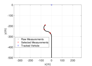
(a) 10 measurements selected.

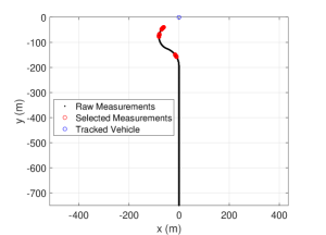
(b) 50 measurements selected.

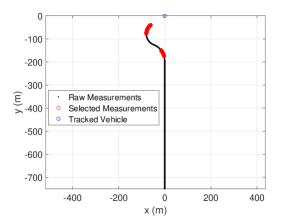
(c) 100 measurements selected.

Figure 2: Example 1, where 1000 total measurements are collected uniformly along the path shown in black. Small subsets of measurements are selected using the proposed methodology and are shown in red. The ground-truth location of the object to be tracked is marked in blue.

The sensing agent has an on-board camera and associated image-processing algorithms that determine the target’s image coordinates. Assuming a projective camera model with optical center at the agent’s position $p(\tau_{k})$ and a (known) camera orientation $R_{c}(\tau_{k})$, the target’s image coordinates at time $\tau_{k}\in\left[t_{\ell-1},t_{\ell}\right]$ are given as [15, Chapter. 5, p. 141]

$${\mathcal{I}}\left(\tau_{k}\right)=\frac{M\left(\tau_{k}\right)\left(q\left(\tau_{k}\right)-p\left(\tau_{k}\right)\right)}{m\left(\tau_{k}\right)\left(q\left(\tau_{k}\right)-p\left(\tau_{k}\right)\right)},$$ (23)

where

$$M\left(t\right):=\left[\begin{array}[]{ccc}1&0&0\\ 0&1&0\end{array}\right]AR_{c}\left(t\right),$$

and

$$m\left(t\right):=\left[\begin{array}[]{ccc}0&0&1\end{array}\right]AR_{c}\left(t\right),$$

and $A$ denotes the camera’s intrinsic parameters matrix, which is defined as

$$A=\left[\begin{array}[]{ccc}f_{x}&s_{xy}&o_{x}\\ 0&f_{y}&o_{y}\\ 0&0&1\end{array}\right],$$

where $f_{u}$, $f_{v}$ are the camera focal lengths in the $x$, and $y$ directions, respectively, in the image plane; $\left(o_{x},o_{y}\right)$ is the focal center of the image plane and $s_{xy}$ is the skew parameter. We regard the target’s image coordinates produced by the image processing algorithms as Gaussian random vectors in ${\mathbb{R}}^{2}$ with means given by $\left(\ref{eq:image projection}\right)$ and covariance matrix $\Sigma_{{\mathcal{I}}}$ independent of the unknown parameters, which means that the likelihood of a measurement $y_{k}$ of $\left(\ref{eq:image projection}\right)$ is given by

$$P\left(y_{k};\Sigma_{{\mathcal{I}}}\right)=\frac{1}{2\pi\sqrt{\det\Sigma_{{\mathcal{I}}}}}e^{-\frac{1}{2}\left({\mathcal{I}}\left(\tau_{k}\right)-y_{k}\right)^{\top}\Sigma_{{\mathcal{I}}}\left({\mathcal{I}}\left(\tau_{k}\right)-y_{k}\right)}.$$

For the motion model in $\left(\ref{eq:motion model}\right)$, the gradient with respect to the motion parameters is given by

$$\frac{\partial{\mathcal{I}}\left(\tau_{k}\right)}{\partial\theta_{1}}=\frac{M\left(\tau_{k}\right)}{d\left(\tau_{k}\right)}-\frac{U\left(\tau_{k}\right)}{d\left(\tau_{k}\right)^{2}}m\left(\tau_{k}\right),$$

and

$$\frac{\partial{\mathcal{I}}\left(\tau_{k}\right)}{\partial\theta_{2}}=\left(\tau_{k}-t_{k-1}\right)\left(\frac{M\left(\tau_{k}\right)}{d\left(\tau_{k}\right)}-\frac{U\left(\tau_{k}\right)}{d\left(\tau_{k}\right)^{2}}m\left(\tau_{k}\right)\right),$$

and

$$\frac{\partial{\mathcal{I}}\left(\tau_{k}\right)}{\partial\theta_{3}}=\frac{\left(\tau_{k}-t_{k-1}\right)^{2}}{2}\left(\frac{M\left(\tau_{k}\right)}{d\left(\tau_{k}\right)}-\frac{U\left(\tau_{k}\right)}{d\left(\tau_{k}\right)^{2}}m\left(\tau_{k}\right)\right),$$

where

$$U\left(t\right):=M\left(t\right)\left(q\left(t\right)-p\left(t\right)\right),$$

and

$$d\left(t\right):=m\left(t\right)\left(q\left(t\right)-p\left(t\right)\right).$$

6 Results

This section contains several examples based on synthetic data that illustrate the benefits of FIM-based measurement selection.

6.1 Example 1: A Single Camera

Our first example is that of an agent with a single imaging sensor, measuring the position of a stationary vehicle in the image plane as described in Sec. 5.3. The camera has a focal length of 50 pixels and image-plane noise with a standard deviation of $0.8$ pixels. An agent follows the path show in Fig. 2. This example highlights how the FIM can be used to asses how informative each of the vision measurements are. In this instance, when the path is facing straight at the object then little information is gained in the ’y’ direction since any single image cannot measure depth. However, when multiple images are captured at different angles relative to the object, then depth can be estimated. The FIM quantifies this phenomenon and we can optimally pick the most informative subset of measurements. This is shown in Fig. 2 where 1000 measurements are uniformly collected along the agent’s path and a small subset of measurements are selected using Algorithm 1 to pick those measurements that minimally reduce the degradation of estimation performance as compared to the full set of collected measurements. The FIM-selected measurements provide a compromise between closeness to the target (which is maximal right at the end of the path) and largest diversity of viewing angle. We use the unscented transform [16, 17] to estimate the parameters and the resulting estimation error is shown in Figure 3, though other state-of-the-art estimation schemes designed specifically for tracking could also be utilized such as interacting multiple model methods [18] or changepoint filtering [19]. Figure 3 shows tremendous reduction in estimation error when using FIM-based selection instead of random selection for regimes with very few measurements selected.

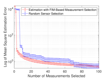
Figure 3: Averaged estimation error versus the number of measurements selected for Example 1. Red shows the average estimation error using measurement selected using the FIM-based method in Algorithm 1 and blue show the average estimation error using a random selection.

6.2 Example 2: Two Heterogeneous Sensors

The next example is based on similar trajectories for the vehicle and mobile agent as in Example 1, but the latter has an additional RF sensor that measures the Doppler shift, as in Section 5.2, with a noise standard deviation of 33ppb in frequency. The agent uses the FIM-based criteria to select a mixture of measurements between the two sensors.

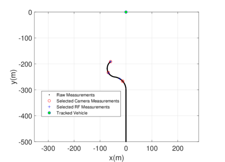
(a) 10 measurements selected from 1000 measurements collected each from a camera and RF sensor.

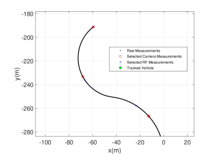
(b) Zoomed to show detail of the measurements selected during the final section of the trajectory.

Figure 4: Example 2, where 1000 total measurements are collected each from a camera and RF sensor, uniformly along the path shown in black. A subset of 10 measurements are selected between the sensors using the proposed methodology. Selected camera measurements are shown red and selected RF measurements are shown in blue. 7 vision measurements and 3 RF measurements were selected out of 1000 total available. The ground-truth location of the object to be tracked is marked in green.

The performance is compared to randomly selecting measurements and is shown in the Figure 5a, where we see a dramatic reduction in estimation estimation error with just a small number of measurements selected. Figure 5b shows the ratio of image measurements to RF measurements selected. Where we can see that, for this geometry FIM-based selections roughly pick 2/3 of the measurements from the camera versus 1/3 from the radio receiver.

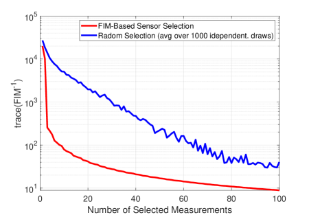
(a) Performance versus the number of total measurements selected from a pool of 1000 measurements collected each from a camera and RF sensor.

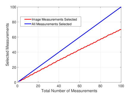
(b) Ratio of RF and image measurements selected.

Figure 5: Example 2, where measurements are jointly selected from two heterogeneous sensors.

6.3 Example 3: Multiple Platforms

We expand on Example 2 by having two agents, each with a camera and RF sensor measuring frequency shifts. Each agent selects a mixture of camera and RF measurements based in Algorithm 1 and sends it to a centralized node for processing. Figure 6 shows which measurements are selected from each agent. The error covariance versus the number of measurements selected by each agent is shown in Figure 7. Compared to estimation with only a single agent, multiple independent agents performing FIM-based measurement selection performs better.

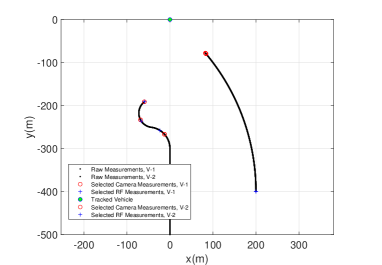
Figure 6: Example 3, where each of the 2 agents collects 1000 total measurements each from a camera and RF sensor, uniformly along the paths shown in black. A subset of 10 measurements are selected between the sensors using the proposed methodology from each agent. Selected camera measurements are shown red and selected RF measurements are shown in blue. The ground-truth location of the object to be tracked is marked in green.

6.4 Cooperative Measurement Selection

The measurement selection algorithm provided by Algorithm 1 operates independently across agents and therefore does not require inter-agent communication. However, when communication between agents is available, there is opportunity for further performance improvement, even when only a small amount of information can be exchanged between agents.

Consider Example 3 above, but after agent 1 chooses a set of measurements, the FIM matrix $\text{FIM}\left(F_{i}^{*}\right)$ is shared with agent 2 to use as a replacement of $Q_{0}$ in its local selection of measurements, $F_{2}^{*}$. This allows the consideration of agent 1’s selection to aid in selecting a better subset from agent 2. The result is a substantial decrease in estimation error compared to the independent selection and is shown in Figure 7.

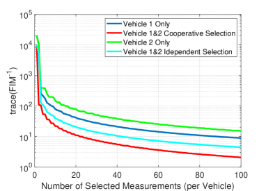
Figure 7: Estimation error performance using only the given number of measurements selected using the FIM-based approached. The blue and green show the performance for using only agent 1 or 2, respectively. The cyan curve is the performance when both are used at the centralized node to improve estimation after being selected independently with a FIM-based criteria. Red is the performance when cooperative FIM-based measurement selection is performed.

7 Conclusions and Future Work

We presented a FIM-based submodular criteria to select measurements for near-optimal estimation performance in a computationally efficient manor. We construct the FIM for several sensors that are commonly used in vehicle tracking problems. Future work includes establishing theoretical guarantees for cooperative sensor selection and validation on experimental data. We have preliminary results showing that the cooperative algorithm outlined in Section 6.4 provides theoretical guarantees of performance when compared to the optimal centralized algorithm.

Matthew R. KirchnerThumbnail.jpg received his B.S. in Mechanical Engineering from Washington State University in 2007 and his M.S. in Electrical Engineering from the University of Colorado at Boulder in 2013. He joined the Naval Air Warfare Center Weapons Division in 2007 and since 2012 has been with the Image and Signal Processing Branch in the Research Directorate, Code 4F0000D. He is currently a Ph.D. student in the Electrical and Computer Engineering Department at the University of California, Santa Barbara. His research interests include level set methods for optimal control, differential games, and reachability; multi-vehicle robotics; nonparametric signal and image processing; and navigation and flight control. He was the recipient of a Naval Air Warfare Center Weapons Division Graduate Academic Fellowship from 2010 to 2012 and in 2011 was named a Paul Harris Fellow by Rotary International. Matthew is a student member of the IEEE.

João P. HespanhaJoao_Office_Ratio.jpg received his Ph.D. degree in electrical engineering and applied science from Yale University, New Haven, Connecticut in 1998. From 1999 to 2001, he was Assistant Professor at the University of Southern California, Los Angeles. He moved to the University of California, Santa Barbara in 2002, where he currently holds a Professor position with the Department of Electrical and Computer Engineering. Dr. Hespanha is the recipient of the Yale University’s Henry Prentiss Becton Graduate Prize for exceptional achievement in research in Engineering and Applied Science, the 2005 Automatica Theory/Methodology best paper prize, the 2006 George S. Axelby Outstanding Paper Award, and the 2009 Ruberti Young Researcher Prize. Dr. Hespanha is a Fellow of the IEEE and he was an IEEE distinguished lecturer from 2007 to 2013. His current research interests include hybrid and switched systems; multi-agent control systems; distributed control over communication networks (also known as networked control systems); the use of vision in feedback control; stochastic modeling in biology; and network security.

Denis GaragićPictureDG.png is a Chief Scientist at BAE Systems FAST Labs. He is a key innovator, guiding FAST Labs’s creation of cognitive computing solutions that provide machine intelligence and anticipatory intelligence to solve challenges across any domain for multiple United States Department of Defense customers including DARPA, the services, and the intelligence community. Denis has 20 years of experience in the areas of autonomous cooperative control for unmanned vehicles; game theory for distributed and hierarchical multilevel decision-making, agent-based modeling and simulation; artificial intelligence and machine learning for multi-sensor data fusion, complex scene understanding, motion activity pattern learning and prediction, learning communications signal behavior, speech recognition, and automated text generation. He received his B.S. and M.S. (Mechanical Engineering and Technical Cybernetics; Applied Mathematics) degrees from The Czech Technical University, Prague, Czech Republic, and his Ph.D. in Mechanical Engineering – System Dynamics and Controls from The Ohio State University.

References

• [1] T. H. Cormen, C. E. Leiserson, R. L. Rivest, and C. Stein, Introduction to Algorithms, 3rd ed.   MIT press, 2009.
• [2] M. Shamaiah, S. Banerjee, and H. Vikalo, “Greedy sensor selection: Leveraging submodularity,” in 49th IEEE Conference on Decision and Control (CDC).   IEEE, 2010, pp. 2572–2577.
• [3] S. T. Jawaid and S. L. Smith, “Submodularity and greedy algorithms in sensor scheduling for linear dynamical systems,” Automatica, vol. 61, pp. 282–288, 2015.
• [4] A. Krause and C. Guestrin, “Near-optimal observation selection using submodular functions,” in AAAI, vol. 7, 2007, pp. 1650–1654.
• [5] A. Krause, H. B. McMahan, C. Guestrin, and A. Gupta, “Robust submodular observation selection,” Journal of Machine Learning Research, vol. 9, no. Dec, pp. 2761–2801, 2008.
• [6] S. Thrun, W. Burgard, and D. Fox, Probabilistic Robotics.   MIT Press, 2005.
• [7] S. Shankar, K. Ezal, and J. P. Hespanha, “Finite horizon maximum likelihood estimation for integrated navigation with RF beacon measurements,” Asian Journal of Control, vol. 21, no. 4, pp. 1470–1482, 2019.
• [8] F. Bian, D. Kempe, and R. Govindan, “Utility based sensor selection,” in Proceedings of the 5th International Conference on Information Processing in Sensor Networks.   ACM, 2006, pp. 11–18.
• [9] W. J. Welch, “Branch-and-bound search for experimental designs based on D-optimality and other criteria,” Technometrics, vol. 24, no. 1, pp. 41–48, 1982.
• [10] S. Joshi and S. Boyd, “Sensor selection via convex optimization,” IEEE Transactions on Signal Processing, vol. 57, no. 2, pp. 451–462, 2008.
• [11] R. D. Gill and B. Y. Levit, “Applications of the van Trees inequality: A Bayesian cramér-Rao bound,” Bernoulli, vol. 1, no. 1-2, pp. 59–79, 1995.
• [12] T. H. Summers, F. L. Cortesi, and J. Lygeros, “Corrections to "On submodularity and controllability in complex dynamical networks",” IEEE Transactions on Control of Network Systems, vol. 5, no. 3, pp. 1503–1503, 2018.
• [13] G. L. Nemhauser, L. A. Wolsey, and M. L. Fisher, “An analysis of approximations for maximizing submodular set functions-I,” Mathematical Programming, vol. 14, no. 1, pp. 265–294, 1978.
• [14] L. Malagò and G. Pistone, “Information geometry of the gaussian distribution in view of stochastic optimization,” in Proceedings of the 2015 ACM Conference on Foundations of Genetic Algorithms XIII.   ACM, 2015, pp. 150–162.
• [15] R. Hartley and A. Zisserman, Multiple View Geometry in Computer Vision.   Cambridge University Press, 2003.
• [16] E. A. Wan and R. Van Der Merwe, “The unscented Kalman filter for nonlinear estimation,” in Proceedings of the IEEE 2000 Adaptive Systems for Signal Processing, Communications, and Control Symposium.   IEEE, 2000, pp. 153–158.
• [17] S. J. Julier, “The scaled unscented transformation,” in Proceedings of the 2002 American Control Conference, vol. 6.   IEEE, 2002, pp. 4555–4559.
• [18] E. Mazor, A. Averbuch, Y. Bar-Shalom, and J. Dayan, “Interacting multiple model methods in target tracking: A survey,” IEEE Transactions on Aerospace and Electronic Systems, vol. 34, no. 1, pp. 103–123, 1998.
• [19] M. R. Kirchner, K. Ryan, and N. Wright, “Maneuvering vehicle tracking with Bayesian changepoint detection,” in 2017 IEEE Aerospace Conference.   IEEE, 2017, pp. 1–9.
\thebiography{biographywithpic}