New travelling wave solutions of the Porous-Fisher model with a moving boundary

Abstract

We examine travelling wave solutions of the Porous-Fisher model, $\partial_{t}u(x,t)=u(x,t)\left[1-u(x,t)\right]+\partial_{x}\left[u(x,t)\partial_{x}u(x,t)\right]$, with a Stefan-like condition at the moving front, $x=L(t)$. Travelling wave solutions of this model have several novel characteristics. These travelling wave solutions: (i) move with a speed that is slower than the more standard Porous-Fisher model, $c<1/\sqrt{2}$; (ii) never lead to population extinction; (iii) have compact support and a well-defined moving front, and (iv) the travelling wave profiles have an infinite slope at the moving front. Using asymptotic analysis in two distinct parameter regimes, $c\to 0^{+}$ and $c\to 1/\sqrt{2}\,^{-}$, we obtain closed-form mathematical expressions for the travelling wave shape and speed. These approximations compare well with numerical solutions of the full problem.

Keywords: Fisher’s equation , nonlinear degenerate diffusion, Stefan condition, moving boundary problem

1 Introduction

Travelling waves arise in many fields, including ecology [1, 2, 3, 4], cell biology[5, 6, 7, 8, 9, 10, 11], and industrial applications involving heat and mass transfer [12, 13, 14, 15]. Such processes are often modelled using reaction-diffusion equations and, depending on the choice of reaction and diffusion terms, three broad classes of monotone travelling waves are commonly reported (Figure 1). The most commonly-observed travelling wave is a smooth front (Figure 1a), whereby the concentration, $u(x,t)$, is a monotone decreasing function decaying to zero as $x\to\infty$. For example, travelling wave solutions of the Fisher-KPP model [1, 2, 7],

$$\partial_{t}u(x,t)=u(x,t)\left[1-u(x,t)\right]+\partial_{xx}u(x,t),\qquad-\infty<x<\infty,$$ (1)

are smooth. Unfortunately, smooth fronts do not have compact support, which makes defining the “edge” of the moving front ambiguous [8, 9, 16]. This feature of the Fisher-KPP model means that it can be hard to apply to practical problems, such as cell invasion [7, 8, 9], where well-defined fronts are often observed.

Figure 1: Schematic representation of various monotone travelling waves.

To obtain travelling wave solutiuons with a well-defined front, two main modifications of the Fisher-KPP model have been proposed. The first modification involves incorporating nonlinear degenerate diffusion, whereby the concentration flux is generalized to $-D(u)\partial_{x}u$, with $D(0)=0$. One common choice of degenerate diffusivity is $D(u)\equiv u$, which leads to the Porous-Fisher model [10, 17, 18, 19, 20, 21, 22, 23, 11]:

$$\partial_{t}u(x,t)=u(x,t)\left[1-u(x,t)\right]+\partial_{x}\left[u(x,t)\partial_{x}u(x,t)\right],\qquad-\infty<x<\infty.$$ (2)

The Porous-Fisher model supports travelling wave solutions that move with speed $c\geq c_{\textrm{min}}$, where $c_{\textrm{min}}=1/\sqrt{2}$ [1, 19, 20, 24]. Phase plane analysis shows that travelling wave solutions of the Porous-Fisher model are sharp-fronted, with compact support, when $c=1/\sqrt{2}$ [1, 20, 24]. In contrast, travelling wave solutions of the Porous-Fisher model with $c>1/\sqrt{2}$ are smooth and do not have compact support [1, 24]. Interestingly, travelling wave solutions of the Porous-Fisher model with $c<1/\sqrt{2}$ have never been reported.

The second modification of the Fisher-KPP model that leads to a well-defined front is to maintain the use of linear diffusion, but to incorporate a moving boundary condition so that we consider the Fisher-KPP model on $-\infty<x<L(t)$ [25, 4, 7]. This second modification of the Fisher-KPP model has been called the Fisher-Stefan model [25, 7], which incorporates a Stefan-like condition at the moving boundary, $L(t)$, to relate the concentration flux, $-\partial_{x}u(x,t)$, with the speed of the moving boundary. One of the limitations of the Fisher-Stefan model is that this model allows populations to become extinct [25, 7], since there is an outward flux of at the leading edge, $x=L(t)$. While the Fisher-Stefan model has the advantage that it can lead to sharp-fronted travelling waves, the physical or biological explanation of the outward flux at $x=L(t)$ is not obvious.

Both the Porous-Fisher and the Fisher-Stefan models have the advantage that they lead to travelling wave solutions with a well-defined front (Figure 1b,c). While these two modifications of the Fisher-KPP model have been considered previously, the extension of combining nonlinear degenerate diffusion with a moving boundary condition has yet to be considered. We refer to this combination of the Porous-Fisher model with a moving boundary condition as the Porous-Fisher-Stefan model, which we define as the Porous-Fisher equation (2) on $x\in(-\infty,L(t)]$ with a Stefan-like condition stating that the speed of the moving front, $\mathrm{d}L(t)/\mathrm{d}t$, is proportional to the nonlinear concentration flux, $-u(x,t)\partial_{x}u(x,t)$, with constant of proportionality $\kappa>0$. Unlike the Fisher-Stefan model [25, 7], the incorporation of nonlinear degenerate diffusion in the Porous-Fisher-Stefan model prevents $u(x,t)$ from being driven to extinction. Interestingly, preliminary numerical solutions of the Porous-Fisher-Stefan model suggest that travelling wave solutions exist with $0\leq c<1/\sqrt{2}$ and that these sharp-fronted travelling waves have infinite slope at $x=L(t)$ (Figure 1d). Neither of these properties have been reported or analyzed previously.

In this work, we examine sharp-fronted travelling waves that arise in the Porous-Fisher-Stefan model. By transforming this model into travelling wave coordinates, we examine the phase plane for various regimes of the wave speed $c$. Using asymptotic analysis, we obtain approximations of the resulting phase plane trajectories when $c\ll 1$ and when $c$ is close to the critical wave speed $1/\sqrt{2}$. Additionally, we determine the relationship between the travelling wave speed $c$ and the Stefan parameter $\kappa$. In doing so, we determine an approximate form of the travelling wave front that matches numerically-computed travelling wave solutions with high accuracy.

2 Travelling waves in the Porous-Fisher-Stefan model

We consider the non-dimensional Porous-Fisher model, describing the concentration $u(x,t)\in[0,1]$ with a Stefan-like condition at the moving boundary $x=L(t)$:

$$\partial_{t}u(x,t)=u(x,t)\left[1-u(x,t)\right] +\partial_{x}\left[u(x,t)\partial_{x}u(x,t)\right],\qquad-\infty<x<L(t),$$ (3)

$$\lim_{x\to-\infty} u(x,t)=1,\qquad u(L(t),t)=0,$$ (4)

$$\frac{\mathrm{d}L(t)}{\mathrm{d}t}=-\kappa \left.u(x,t)\partial_{x}u(x,t)\right|_{x\to L(t)^{-}},\qquad L(0)=L_{0}.$$ (5)

The Stefan-like condition relates the speed of the moving front, $\mathrm{d}L(t)/\mathrm{d}t$, to the concentration flux, $-u(x,t)\partial_{x}u(x,t)$, via the constant $\kappa>0$. Preliminary numerical solutions of (3)–(5) suggest that travelling waves exist and that these waves move with speed $0\leq c<1/\sqrt{2}$ with infinite gradient at $x=L(t)$. Consequently, we are motivated to examine travelling wave solutions of the Porous-Fisher-Stefan model and to determine the relationship between $c$ and $\kappa$. To do this, we define $\phi(x,t)=[u(x,t)]^{2}$ to obtain a corresponding PDE with a linear Stefan-like condition at $x=L(t)$:

$$\partial_{t}\phi(x,t)=2\phi(x,t)\left[1-\sqrt{\phi(x,t)}\right] +\sqrt{\phi(x,t)}\,\partial_{xx}\phi(x,t),\qquad-\infty<x<L(t),$$ (6)

$$\lim_{x\to-\infty} \phi(x,t)=1,\qquad\phi(L(t),t)=0,$$ (7)

$$\frac{\mathrm{d}L(t)}{\mathrm{d}t}=- \frac{\kappa}{2}\left.\partial_{x}\phi(x,t)\right|_{x\to L(t)^{-}},\qquad L(0)=L_{0}.$$ (8)

To study travelling wave solutions of (6)–(8), we transform the system into travelling wave coordinates via $z=x-L_{0}-ct,$ where $z\in(-\infty,0]$. Noting that when $x=L(t)$, we have $L(t)=L_{0}+ct$, and hence, $\mathrm{d}L(t)/\mathrm{d}t=c$. This change of coordinates gives

$$\sqrt{\phi(z)}\,\phi^{\prime\prime}(z)+ c\phi^{\prime}(z)+2\phi(z)\left(1-\sqrt{\phi(z)}\right)=0,\qquad-\infty<z<0,$$ (9)

$$\lim_{z\to-\infty}\phi(z)=1,\quad \phi(0)=0,\quad\lim_{z\to 0^{-}}\phi^{\prime}(z)=-\frac{2c}{\kappa},$$ (10)

where ${}^{\prime}=\mathrm{d}/\mathrm{d}z$. It is convenient to write (9) as a system of two first order differential equations:

$$\phi^{\prime}(z) =\psi(z),$$ (11)

$$\psi^{\prime}(z) =-\frac{c\psi(z)}{\sqrt{\phi(z)}}-2\sqrt{\phi(z)}\left(1-\sqrt{\phi(z)}\right).$$ (12)

A general explicit solution of (11)–(12) is not obvious, so we seek to study solutions of this system using the $(\phi(z),\psi(z))$ phase plane. There are only two fixed points of (11)–(12): $(0,0)$ and $(1,0)$. Typically, with phase plane analysis of travelling wave solutions, we explore the possibility of a heteroclinic orbit between these fixed points by considering the local behaviour of the linearized system near the fixed points [1, 23]. For the Porous-Fisher model, whose phase plane is identical to (11)–(12), such heteroclinic orbits can only occur for $c\geq 1/\sqrt{2}$ [1, 24]. However, for the Porous-Fisher-Stefan model, we have the addition of the Stefan-like condition in (10). Therefore, travelling wave solutions of the Porous-Fisher-Stefan model do not correspond to a heteroclinc orbit between $(0,0)$ and $(1,0)$, but rather a trajectory between $(1,0)$ and another point that is determined by the moving boundary condition in (10). This particular trajectory, $\psi(\phi;c)$, corresponds to the travelling wave solution for a given $c$ with $\displaystyle\lim_{z\to-\infty}\phi(z)=1$, as well as determining $\kappa$ via (10): $\kappa=-2c/\psi(0;c)$.

To determine $\psi(\phi;c)$, we divide (12) by (11) and obtain

$$-\frac{\mathrm{d}\psi(\phi)}{\mathrm{d}\phi}=\frac{c}{\sqrt{\phi}}+\frac{2\sqrt{\phi}\left(1-\sqrt{\phi}\right)}{\psi(\phi)},\qquad\psi(1)=0,\qquad\lim_{\phi\to 0^{+}}\psi(\phi)=-\frac{2c}{\kappa}.$$ (13)

As previously mentioned, physical travelling wave solutions in the Porous-Fisher model can only occur when $c\geq 1/\sqrt{2}$ [1, 24], and numerical simulations of the Porous-Fisher-Stefan model indicate that all travelling waves have $c<1/\sqrt{2}$. As a result, we examine (13) in two limiting regimes: $c\to 0^{+}$ and $c\to 1/\sqrt{2}\,^{-}$.

2.1 Travelling wave solutions for $c\ll 1$

We first consider the solution of (13) in the limit where $0\leq c\ll 1$ by expanding $\psi(\phi)$ as a regular perturbation expansion in $c$, i.e. $\psi(\phi)=V_{0}(\phi)+cV_{1}(\phi)+\mathcal{O}(c^{2})$. Substituting this expansion into (13) provides

$$\mathcal{O}(1):\qquad-V_{0}(\phi)\frac{\mathrm{d}V_{0}(\phi)}{\mathrm{d}\phi}=2\sqrt{\phi}\left(1-\sqrt{\phi}\right), V_{0}(1)=0,$$ (14)

$$\mathcal{O}(c):\qquad-V_{1}(\phi)\frac{\mathrm{d}V_{0}(\phi)}{\mathrm{d}\phi}-V_{0}(\phi)\frac{\mathrm{d}V_{1}(\phi)}{\mathrm{d}\phi}=\frac{V_{0}(\phi)}{\sqrt{\phi}}, V_{1}(1)=0.$$ (15)

The solution of (14)–(15) are

$$V_{0}(\phi)=-\sqrt{\frac{2}{3}-\frac{8}{3}\phi^{3/2}+2\phi^{2}}~{}~{}\text{ and }~{}~{}V_{1}(\phi)=-\frac{1}{V_{0}(\phi)}\int_{\phi}^{1}\sqrt{\frac{2}{3s}-\frac{8}{3}\sqrt{s}+2s}\,\mathrm{d}s.$$ (16)

Evaluating these expressions at $\phi=0$ gives a two-term approximation for the wave speed $c$ as a function of $\kappa$, provided that $c\ll 1$:

$$\kappa\sim\frac{54\sqrt{3}c}{27\sqrt{2}-\alpha c}\iff c\sim\frac{27\sqrt{2}\kappa}{54\sqrt{3}+\alpha\kappa},$$ (17)

where $\alpha=36\sqrt{2}-6\sqrt{3}+24\log[(\sqrt{3}-1)/(3\sqrt{2}-4)]\approx 67.02$. We note that since $\psi=2uu^{\prime}$ remains $\mathcal{O}(1)$ as $\phi\to 0^{+}$, this implies that $u^{\prime}=\mathcal{O}(u^{-1})$ as $u\to 0^{+}$, confirming that we are examining a new class of travelling wave solutions with infinite slope at the moving boundary.

2.2 Travelling wave solutions for $c\to 1/\sqrt{2}\,^{-}$

From [1, 20, 24], we know that when $c=1/\sqrt{2}$, (13) has the solution $u^{\prime}=(u-1)/\sqrt{2}$, implying that $\psi=2uu^{\prime}\to 0$ as $u\to 0^{+}$. The Stefan-like condition in (13) requires that $-2c/\kappa$ must also equal zero. Since $c\neq 0$, this implies that $\kappa\to\infty$ as $c\to 1/\sqrt{2}\,^{-}$. To determine the leading-order behaviour of $\kappa$ in this limit, we let $c=1/\sqrt{2}-\varepsilon$, with $0\leq\varepsilon\ll 1$, and (13) becomes

$$-\frac{\mathrm{d}\psi(\phi)}{\mathrm{d}\phi}=\frac{1}{\sqrt{2\phi}}-\frac{\varepsilon}{\sqrt{\phi}}+\frac{2\sqrt{\phi}\left(1-\sqrt{\phi}\right)}{\psi(\phi)},\quad\psi(1)=0,\quad\lim_{\phi\to 0^{+}}\psi(\phi)=-\frac{2}{\kappa}\left(\frac{1}{\sqrt{2}}-\varepsilon\right).$$ (18)

We perform a regular perturbation expansion in $\varepsilon$, i.e. $\psi=\Psi_{0}(\phi)+\varepsilon\Psi_{1}(\phi)+\mathcal{O}(\varepsilon^{2})$, which gives

$$\mathcal{O}(1):\qquad-\frac{\mathrm{d}\Psi_{0}(\phi)}{\mathrm{d}\phi}=\frac{1}{\sqrt{2\phi}}+\frac{2\sqrt{\phi}\left(1-\sqrt{\phi}\right)}{\Psi_{0}(\phi)},\qquad \Psi_{0}(1)=0,$$ (19)

$$\mathcal{O}(\varepsilon):\qquad-\Psi_{1}(\phi)\frac{\mathrm{d}\Psi_{0}(\phi)}{\mathrm{d}\phi}-\Psi_{0}(\phi)\frac{\mathrm{d}\Psi_{1}(\phi)}{\mathrm{d}\phi}=\frac{\Psi_{1}(\phi)}{\sqrt{2\phi}}-\frac{\Psi_{0}(\phi)}{\sqrt{\phi}},\qquad \Psi_{1}(1)=0.$$ (20)

Noting that $u_{0}^{\prime}=(u_{0}-1)/\sqrt{2}$ is the leading-order solution in the original variables, the solutions of (19)–(20) are

$$\Psi_{0}(\phi)=2u_{0}u^{\prime}_{0}=-\sqrt{2\phi}\left(1-\sqrt{\phi}\right)~{}~{}\text{ and }~{}~{}\Psi_{1}(\phi)=-\frac{2\left(1-\sqrt{\phi}\right)}{3}.$$ (21)

Evaluating $\Psi_{0},\Psi_{1}$ at $\phi=0$ retrieves the Stefan-like condition in (18); hence, for $c=1/\sqrt{2}-\varepsilon$, corresponding to $\kappa\gg 1$, we have

$$\kappa\sim\frac{3\sqrt{2}c}{1-\sqrt{2}c}\iff c\sim\frac{\kappa}{\sqrt{2}\,(\kappa+3)}.$$ (22)

In the limit where $\kappa\gg 1$, we can also approximate the travelling wave front $\phi(z)$. To do this, we note that

$$\frac{\mathrm{d}\phi}{\mathrm{d}z}\sim\Psi_{0}(\phi)+\varepsilon\Psi_{1}(\phi)=\sqrt{2}\left(\sqrt{\phi}-1\right)\left(\sqrt{\phi}+\frac{\varepsilon\sqrt{2}}{3}\right),\qquad\phi(0)=0,$$ (23)

with solution

$$z(\phi)=\frac{3\sqrt{2}}{3+\varepsilon\sqrt{2}}\left[\log\left(1-\sqrt{\phi}\right)+\frac{\varepsilon\sqrt{2}}{3}\log\left(1+\frac{3}{\varepsilon}\sqrt{\frac{\phi}{2}}\right)\right].$$ (24)

Equivalently, the original travelling wave $u(z)=\sqrt{\phi(z)}$ can be written implicitly, using (22), as

$$z(u)\sim\frac{(\kappa+3)\sqrt{2}}{\kappa+4}\left[\log\left(1-u\right)+\frac{\log\left(1+(\kappa+3)u\right)}{\kappa+3}\right].$$ (25)

Thus, we can approximate the sharp moving front $u(z)$, along with its corresponding wave speed $c$, in the regime where $\kappa$ is large. Furthermore, we note that in the limit where $\kappa\to\infty$, we have $z(u)\to\sqrt{2}\log(1-u)$, implying that $u(z)=1-\exp\left(z/\sqrt{2}\right)$. This result agrees with the sharp-fronted travelling wave determined in [1, 20, 24].

2.3 Comparison of travelling wave solutions

To validate our asymptotic approximations, we firstly examine the trajectory $\psi(\phi;c)$, which solves (13) for a given $c$, in the $(\phi,\psi)$-phase plane. To determine $\psi(\phi;c)$, we solve (13) numerically using ode45 in MATLAB. In Figure 2a, the two-term approximation $V_{0}(\phi)+cV_{1}(\phi)$, valid when $c\ll 1$, agrees very well with $\psi(\phi;c)$ up to $c=0.2$. Furthermore, in Figure 2b, we have good agreement between $\psi(\phi;c)$ and the two-term approximation $\Psi_{0}(\phi)+\varepsilon\Psi_{1}(\phi)$, in the limit when $c=1/\sqrt{2}-\varepsilon$ up to $\varepsilon=0.2$.

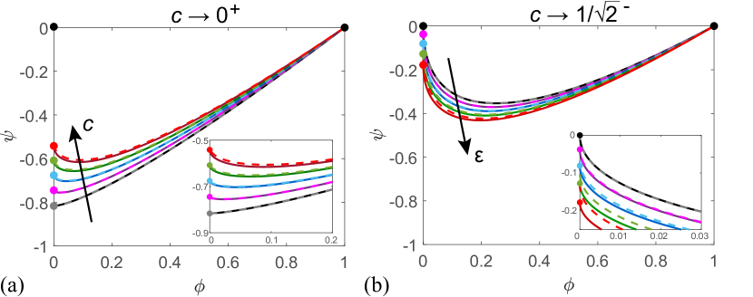
Figure 2: Comparison of the trajectory $\psi(\phi;c)$ in the $(\phi,\psi)$-phase plane (solid curves), which solves (13) for a given $c$, with its two-term asymptotic approximations (dashed curves). The fixed points $(\phi,\psi)=(0,0),(1,0)$ are shown as black circles, while the Stefan-like condition at $\phi=0$ is shown as coloured circles. (a) The two-term asymptotic approximation when $c\ll 1$ is $V_{0}+cV_{1}$, where $c=0$ (black/grey), $c=0.05$ (pink), $c=0.1$ (blue), $c=0.15$ (green), and $c=0.2$ (red). The black arrow points in the direction of increasing $c$. (b) The two-term asymptotic approximation when $c=1/\sqrt{2}-\varepsilon$ is $\Psi_{0}+\varepsilon\Psi_{1}$, where $\varepsilon=0$ (black/grey), $\varepsilon=0.05$ (pink), $\varepsilon=0.1$ (blue), $\varepsilon=0.15$ (green), and $\varepsilon=0.2$ (red). The insets in (a) and (b) show the solutions near $\phi=0$. The black arrow points in the direction of increasing $\varepsilon$.

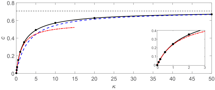
Figure 3: Comparison of the $c(\kappa)$ curves: numerically computed from (6)–(8) (black circles), numerically computed from (13) (black solid curve), and the two-term approximations for $c\ll 1$ (red dot-dash curve) and $\kappa\gg 1$ (blue dashed curve). The critical wave speed $c=1/\sqrt{2}$ is shown as a black dashed line.

Since the asymptotic approximations accurately describe $\psi(\phi;c)$ in the phase plane, we now examine the asymptotic relationship between $c$ and $\kappa$. We can estimate $c(\kappa)$ from the numerically-computed $\psi(\phi;c)$ by noting that $c=-\kappa\,\psi(0;c)/2$. Alternatively, we can use the numerical solutions of (6)–(8) to determine the speed of the moving front $L(t)$, once the solution has settled to the travelling wave solution (see Appendix A). Figure 3 shows that these two numerical approaches to determine $c(\kappa)$ are indeed equivalent. Furthermore, we see that both asymptotic approximations for $c(\kappa)$, (17) and (22), agree with the numerically-determined $c(\kappa)$ relationship. To minimize the error between $c(\kappa)$ and its asymptotic approximations, we recommend that (17) be used for $\kappa<2$ and (22) be used for $\kappa>20$. For intermediate values of $\kappa$, it appears that a numerical solution is warranted.

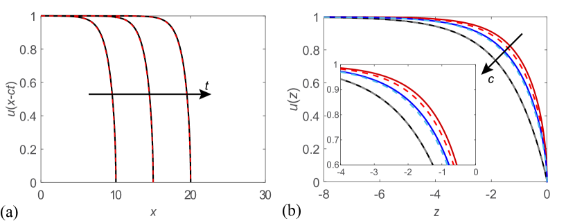
Figure 4: (a) Comparison of the travelling wave front $u(x-ct)$ for $\kappa=1$. The numerical solution of (6)–(8) is shown in black at equally-spaced times ($t=41.0,61.5,82.0$), using (25) as an initial condition. The red-dashed front is determined from large-$\kappa$ asymptotics (25). The black arrow points in the direction of increasing $t$. (b) Travelling wave fronts $u(z)$ (solid curves), superimposed on the corresponding asymptotic approximations (dashed curves) determined using (22) and (25), for $c=0.7$ (black/grey), $c=0.4$ (blue), and $c=0.1$ (red). The corresponding values of $\kappa$ are 287.1 (295.5), 2.711 (3.907), and 0.2958 (0.4941), respectively, where numerically-determined values are shown in the text and asymptotic approximations of $\kappa$ using (22) are shown in parentheses. The black arrow points in the direction of increasing $c$.

Finally, we compare the asymptotic approximation of the moving front $u(z)=u(x-ct)$, shown in (25), with the numerical solution of (6)–(8), after sufficient time has passed such that the travelling wave has formed (Appendix A). Despite the fact that the asymptotic approximation is only expected to match when $\kappa$ is large, we see in Figure 4a that the asymptotic approximation of the shape of the moving fronts, shown implicitly in (25), matches the numerically-determined travelling wave solution very well, even when $\kappa=1$. Furthermore, the asymptotic approximation in (25) agrees well with the numerically-computed travelling wave fronts for a variety of wave speeds (Figure 4b).

3 Conclusions

In this work, we consider new travelling wave solutions for the Porous-Fisher model with a moving boundary. This model has certain features that could be considered to be advantageous over other modifications of the Fisher-KPP model. In summary, the new travelling wave solutions: (i) move with a speed that is slower than the more standard Porous-Fisher model; (ii) never lead to population extinction; (iii) have compact support and a well-defined moving front, and (iv) the travelling wave profiles have an infinite slope at the moving front. Using travelling wave coordinates, we transform the model into a single nonlinear differential equation. The solution of this differential equation, corresponding to a particular trajectory in the associated phase plane, determines the travelling wave front and can be approximated using asymptotic analysis in two limiting parameter regimes. In both cases, we obtain a good approximation of this trajectory, which can also be used to relate the speed of the moving front to $\kappa$, a constant appearing in the Stefan-like condition. Finally, we determine a highly-accurate approximate form of the sharp-fronted travelling wave with infinite slope at the moving boundary, corresponding to solutions with wave speeds $0\leq c<1/\sqrt{2}$.

Further extensions of this Porous-Fisher-Stefan model can also be made. For instance, the asymptotic analysis performed in this work can be extended to include higher-order terms. Another possible extension could be to consider generalizing the nonlinear degenerate diffusivity function to $D(u)=u^{n}$, for some constant $n>0$ [10, 17, 19, 26, 6]. We leave both extensions for future consideration.

Acknowledgements

This work is supported by the Australian Research Council (DP170100474).

Appendix A Numerical Solution for the Porous-Fisher-Stefan model

A MATLAB implementation of the numerical solution of (6)–(8), described below, can be found at https://github.com/nfadai/Fadai_TW2019.

To numerically compute solutions of (6)–(8), we first approximate the semi-infinite domain $(-\infty,L(t)]$ as the finite domain $[0,L(t)]$, provided that $L_{0}>0$. Additionally, we transform (6)–(8) to a fixed-space domain by setting $\xi=x/L(t).$ Consequently,(6)–(8) becomes

$$\partial_{t}\phi(\xi,t)=\frac{\xi}{L(t)}\,\frac{\mathrm{d}L(t)}{\mathrm{d}t}\,\partial_{\xi}\phi(\xi,t)+2\phi(\xi,t)\left[1-\sqrt{\phi(\xi,t)}\right]+\frac{\sqrt{\phi(\xi,t)}}{[L(t)]^{2}}\,\partial_{\xi\xi}\phi(\xi,t),$$ (26)

$$\left.\partial_{\xi}\phi(\xi,t)\right|_{\xi=0}=0,\qquad\phi(1,t)=0,\qquad 0<\xi<1,$$ (27)

$$L(t)\frac{\mathrm{d}L(t)}{\mathrm{d}t}=-\frac{\kappa}{2}\left.\partial_{\xi}\phi(\xi,t)\right|_{\xi=1},\qquad L(0)=L_{0}.$$ (28)

To compute the numerical solution of (26)–(28), we must specify values for $L_{0}$, $\kappa$ and $\phi(\xi,0)$. We obtain numerical solutions of (26) on a uniformly-spaced mesh of $\xi\in[0,1]$, i.e. $\xi_{i}=i\Delta\xi$, $i=0,\dots,N$, where $\Delta\xi=1/N$. We denote $\phi(\xi_{i},t_{j})=\phi_{i}^{n}$ and $L(t_{j})=L_{j}$ for convenience, where $n\geq 1$ is the $n$th Picard iteration estimate at time $t_{j}$. Therefore, to determine $\phi_{i}$, we use

$$\frac{\phi_{i}^{n}-\phi_{i}^{p}}{\Delta t}= \frac{\xi_{i}(L_{j}-L_{j-1})(\phi_{i+1}^{n}-\phi_{i-1}^{n})}{2L_{j}\Delta t\Delta\xi}+2\phi_{i}^{n}\left[1-\sqrt{\phi_{i}^{n-1}}\right]$$ (29)

$$+\frac{(\phi_{i+1}^{n}-2\phi_{i}^{n}+\phi_{i-1}^{n})\sqrt{\phi_{i}^{n-1}}}{(L_{j})^{2}(\Delta\xi)^{2}},$$

$$\phi_{0}^{n}=\phi_{1}^{n},\qquad\phi_{N}^{n}=0.$$ (30)

Here, $\phi_{i}^{p}$ is the solution of $\phi_{i}$ at the previous timestep, $t_{j-1}$, and $\Delta t$ is the timestep. We identify the system (29)–(30) as a tridiagonal matrix in $\phi_{i}^{n}$ at time $t_{j}$, which we can solve efficiently using the Thomas algorithm. This solution is stored as $\boldsymbol{\Phi}_{n}$; if $\displaystyle\max\left|\boldsymbol{\Phi}_{n}-\boldsymbol{\Phi}_{n-1}\right|<\delta$, where $\delta$ is some user-specified tolerance, then the Picard loop terminates and we proceed to updating the moving boundary for the next timestep. Otherwise, $n=n+1$, the solution $\boldsymbol{\Phi}_{n}$ is stored as $\phi_{i}^{n-1}$, and the Picard iteration loop is performed again.

From the fixed-boundary PDE, the Stefan-like condition at $\xi=1$ is

$$L(t)\frac{\mathrm{d}L(t)}{\mathrm{d}t}=-\frac{\kappa}{2}\left.\partial_{\xi}\phi(\xi,t)\right|_{\xi=1},\qquad t\in[t_{j},t_{j+1}],\qquad L(t_{j})=L_{j}.$$ (31)

We approximate $\phi(\xi,t)$ as $\phi(\xi,t_{j})$ during the small interval $t\in[t_{j},t_{j+1}]$, allowing us to explicitly solve (31) to give a closed form approximation for $L(t)$:

$$L(t)=\sqrt{(L_{j})^{2}-\kappa\left.\partial_{\xi}\phi(\xi,t_{j})\right|_{\xi=1}(t-t_{j})},\qquad t_{j}\leq t\leq t_{j+1}.$$ (32)

Therefore, evaluating this expression at $t=t_{j+1}$ and using a second-order finite difference approximation of $\displaystyle\left.\partial_{\xi}\phi(\xi,t_{j})\right|_{\xi=1}$, we obtain the approximation

$$L_{j+1}=\sqrt{(L_{j})^{2}-\frac{\kappa\Delta t(3\phi_{N}^{n}-4\phi_{N-1}^{n}+\phi_{N-2}^{n})}{2\Delta\xi}}.$$ (33)

With these updated values of $L_{j+1}$ and $\boldsymbol{\Phi}_{n}=\phi_{i}^{p}$, we update $t=t+\Delta t$ and $j=j+1$; we then repeat the computation to integrate through the next time increment. The algorithm terminates when $t+\Delta t>t_{f}$, where $t_{f}$ is the user-specified final time. Once sufficient time has passed that the solution settles towards a travelling wave, we expect that $\mathrm{d}L(t)/\mathrm{d}t=c$, so we fit a straight line to our numerical estimate of $L(t)$ and use the slope of that line to provide an estimate of $c$.

References

- [1] Murray JD. Mathematical Biology I: An Introduction. Spring-Verlag; 2003.
- [2] Fisher RA. The wave of advance of advantageous genes. Annals of Eugenics. 1937;7(4):355–369.
- [3] Holmes EE, Lewis MA, Banks JE, Veit RR. Partial differential equations in ecology: spatial interactions and population dynamics. Ecology. 1994;75(1):17–29.
- [4] Bao W, Du Y, Lin Z, Zhu H. Free boundary models for mosquito range movement driven by climate warming. Journal of Mathematical Biology. 2018;76(4):841–875.
- [5] Sherratt JA, Murray JD. Models of epidermal wound healing. Proceedings of the Royal Society B: Biological Sciences. 1990;241(1300):29–36.
- [6] McCue SW, Jin W, Moroney TJ, Lo KY, Chou SE, Simpson MJ. Hole-closing model reveals exponents for nonlinear degenerate diffusivity functions in cell biology. Physica D: Nonlinear Phenomena. 2019;398:130–140.
- [7] El-Hachem M, McCue SW, Jin W, Du Y, Simpson MJ. Revisiting the Fisher–Kolmogorov–Petrovsky–Piskunov equation to interpret the spreading–extinction dichotomy. Proceedings of the Royal Society A: Mathematical, Physical and Engineering Sciences. 2019;475(20190378).
- [8] Maini PK, McElwain DLS, Leavesley DI. Travelling waves in a wound healing assay. Applied Mathematics Letters. 2004;17(5):575–580.
- [9] Maini PK, McElwain DLS, Leavesley DI. Traveling wave model to interpret a wound-healing cell migration assay for human peritoneal mesothelial cells. Tissue Engineering. 2004;10(3–4):475–482.
- [10] Simpson MJ, Landman KA, Hughes BD, Newgreen DF. Looking inside an invasion wave of cells using continuum models: proliferation is the key. Journal of Theoretical Biology. 2006;243(3):343–360.
- [11] Simpson MJ, Baker RE, McCue SW. Models of collective cell spreading with variable cell aspect ratio: a motivation for degenerate diffusion models. Physical Review E. 2011;83(021901).
- [12] McGuinness MJ, Please CP, Fowkes N, McGowan P, Ryder L, Forte D. Modelling the wetting and cooking of a single cereal grain. IMA Journal of Management Mathematics. 2000;11(1):49–70.
- [13] Dalwadi MP, O’Kiely D, Thomson SJ, Khaleque TS, Hall CL. Mathematical modeling of chemical agent removal by reaction with an immiscible cleanser. SIAM Journal on Applied Mathematics. 2017;77(6):1937–1961.
- [14] Fadai NT, Please CP, Van Gorder RA. Asymptotic analysis of a multiphase drying model motivated by coffee bean roasting. SIAM Journal on Applied Mathematics. 2018;78(1):418–436.
- [15] Brosa Planella F, Please CP, Van Gorder RA. Extended Stefan problem for solidification of binary alloys in a finite planar domain. SIAM Journal on Applied Mathematics. 2019;79(3):876–913.
- [16] Treloar KK, Simpson MJ. Sensitivity of edge detection methods for quantifying cell migration assays. PloS One. 2013;8(6):e67389.
- [17] Aronson DG. Density-dependent interaction–diffusion systems. In: Dynamics and modelling of reactive systems. Elsevier; 1980. p. 161–176.
- [18] Harris S. Fisher equation with density-dependent diffusion: special solutions. Journal of Physics A: Mathematical and General. 2004;37(24):6267.
- [19] Gilding BH, Kersner R. A Fisher/KPP-type equation with density-dependent diffusion and convection: travelling-wave solutions. Journal of Physics A: Mathematical and General. 2005;38(15):3367.
- [20] Sánchez Garduno F, Maini PK. An approximation to a sharp type solution of a density-dependent reaction-diffusion equation. Applied Mathematics Letters. 1994;7(1):47–51.
- [21] Witelski TP. Shocks in nonlinear diffusion. Applied Mathematics Letters. 1995;8(5):27–32.
- [22] Witelski TP. Merging traveling waves for the porous-Fisher’s equation. Applied Mathematics Letters. 1995;8(4):57–62.
- [23] Sánchez Garduno F, Maini PK. Traveling wave phenomena in some degenerate reaction-diffusion equations. Journal of Differential Equations. 1995;117(2):281–319.
- [24] Sherratt JA, Marchant BP. Nonsharp travelling wave fronts in the Fisher equation with degenerate nonlinear diffusion. Applied Mathematics Letters. 1996;9(5):33–38.
- [25] Du Y, Lin Z. Spreading-vanishing dichotomy in the diffusive logistic model with a free boundary. SIAM Journal on Mathematical Analysis. 2010;42(1):377–405.
- [26] Wang DS, Zhang ZF. On the integrability of the generalized Fisher-type nonlinear diffusion equations. Journal of Physics A: Mathematical and Theoretical. 2008;42(3):035209.