Classical algorithms, correlation decay, and complex zeros of partition functions of quantum many-body systems

Abstract

Various statistical properties of quantum many-body systems in thermal equilibrium such as the free energy, entropy, and average energy can be obtained from the partition function. The problem of estimating the partition function has been the subject of numerous studies in statistical physics, computer science, and machine learning. The aim of this work is to present a new classical algorithm for estimating the partition function of quantum systems. We achieve this by studying the connection between the hardness of approximating the partition function and the thermal phase transition. In particular, we show the following:

1. We demonstrate a quasi-polynomial time classical algorithm that estimates the partition function of quantum systems above the phase transition point. The running time of this algorithm relies heavily on the locus of the complex zeros of the partition function. Intriguingly, these complex zeros are known to mark where the phase transition occurs. By a result of [Sly10], in the worst case, the same problem is ${\sf{NP}}$-hard below this point. Together with our work, this shows that the transition in the phase of a quantum system is also accompanied by a transition in the hardness of approximation.

2. We show that in a system of $n$ particles at temperatures above the phase transition point, where the complex zeros are far from the real axis, the correlations between two observables whose distance is $\Omega(\log n)$ decay exponentially. We can improve the factor of $\log n$ to a constant when the Hamiltonian has commuting terms or is on a $1$D chain. Previously, the decay of correlations was only proved for translationally-invariant $1$D systems [Ara69] or at very high temperatures [KGK⁺14].

3. We find a deterministic quasi-polynomial time approximation algorithm for the $\mathrm{XXZ}$ model in the ferromagnetic regime at any temperature over arbitrary graphs. Previously, a randomized algorithm was known only for the ferromagnetic $\mathrm{XY}$ model [BG17].

This work is the first rigorous study of the connection between the complex zeros of the partition function and the decay of correlations in quantum many-body systems and extends a seminal work of Dobrushin and Shlosman on classical spin models [DS87]. On the algorithmic side, our result extends the scope of a recent approach due to Barvinok for solving classical counting problems [Bar16a] to quantum many-body problems.

1 Introduction

At low temperatures, the main characteristics of many-body systems in condensed matter physics or quantum chemistry are captured in the structure of the ground state of their Hamiltonian. The computational complexity of estimating the ground state energy has been extensively studied through numerous works. In particular, it has been shown that in the worst case, for many physically relevant systems including even a two-local Hamiltonian on a one-dimensional ($1$D) chain, estimating the ground state energy is QMA-complete [AGIK09]. On the other hand, there is a host of classical algorithms for efficiently estimating the ground state energy in certain restricted examples like a gapped Hamiltonian on a $1$D chain [ALVV17] or a dense interaction graph [BaH13].

While at low temperatures the system is in the vicinity of the ground space, at finite temperatures, the state of the system is a mixture of different excited states. In thermal equilibrium, a quantum system characterized by a local Hamiltonian $H$ is in the Gibbs (or thermal) state $\rho=\exp(-\beta H)/Z_{\beta}(H)$, where $\beta$ is the inverse of temperature and $Z_{\beta}(H)=\operatorname{tr}[\exp(-\beta H)]$ is the partition function of the system. A natural equivalent to the ground energy at finite temperatures is the free energy which is defined as $F_{\beta}(H)=-1/\beta\log Z_{\beta}(H)$. Many useful statistical properties of the system including the free energy and entropy can be obtained from the partition function and its derivatives. However, exactly evaluating the partition function is known to be ${\sf{\#P}}$-hard. Hence in order to characterize the finite-temperature behavior of the system, it is crucial to have efficient algorithms that approximate this quantity.

Our starting point for finding such approximation algorithms is based on the observation that the phenomenon of the thermal phase transition is an obstacle for finding efficient algorithms. Consider a quantum many-body system that consists of $n$ qudits interacting according to a local Hamiltonian $H$. As the temperature of this system increases, meaning $\beta\rightarrow 0$, the Gibbs state $\rho$ approaches the maximally mixed state $\mathds{1}/d^{n}$. Thus, in this case, finding the partition function is trivial since $Z_{\beta=0}(H)=d^{n}$. On the other hand, this problem becomes significantly harder at lower temperatures. In particular, as $\beta\rightarrow\infty$, the Gibbs state approaches the ground space of the Hamiltonian $H$ and the free energy $F_{\beta}(H)$ approaches the ground energy which is known to be ${\sf{QMA}}$-hard to estimate. Hence, we see that the computational hardness of estimating the partition function (or equivalently the free energy) depends on the inverse temperature $\beta$ and goes through a transition from being trivial to ${\sf{QMA}}$-hard as $\beta$ increases.

In statistical physics, however, another transition occurs as $\beta$ increases, namely, the transition in the phase of the system. At the thermal phase transition point, certain physical properties of the system undergo an abrupt change. An example of such a transition is when a magnetic material that consists of a network of interacting spins goes from the ferromagnetic to the paramagnetic phase. In the ferromagnetic phase, most spins are pointing in the same direction and their net magnetic effect is non-zero, whereas in the paramagnetic phase, the spins are distributed equally in opposite directions making their net magnetic effect zero. This transition does not happen gradually as $\beta$ varies. On the contrary, the phase of the system changes suddenly at some critical inverse temperature $\beta_{c}$ known as the phase transition point.

Does the computational hardness of estimating the partition function also undergo an abrupt change at the same transition point? This question has been studied in the context of the classical Ising or hard-core model, and the answer is known to be affirmative. For these systems, there are efficient algorithms for estimating the partition function when $\beta<\beta_{c}$ [Wei06, SST14] whereas by a result of Sly and Sun [SS12, Sly10] the same problem is ${\sf{NP}}$-hard for $\beta>\beta_{c}$.

Hence, it appears that the thermal phase transition poses a barrier to obtaining efficient algorithms, and we need a framework for characterizing this phenomenon. There are at least two methods for such purpose. One, which is the basis of our algorithm, stems from analyzing the locus of the complex zeros of the partition function. Another seemingly different method involves the decay of long-range order in the Gibbs state of the system. In this work, we study the interface between these two methods and their algorithmic implications. In particular, we find a quasi-polynomial time approximation algorithm for the partition function for temperatures far from the complex zeros and show that the correlations in the Gibbs state decay exponentially in the same temperature range. The following section summarizes our results.

1.1 Our main results

1.1.1 The complex zeros of the partition function

In general, the partition function can be written as $Z_{\beta}(H)=\sum_{k}\exp(-\beta E_{k})$, where each $E_{k}$ is an eigenvalue of the Hamiltonian $H$. If $\beta$ is real, the terms $\exp(-\beta E_{k})$ are all strictly positive, and hence the partition function $Z_{\beta}(H)$ is strictly positive itself. However, this changes when $\beta$ is allowed to be complex. In that case, the terms $\exp(-\beta E_{k})$ acquire complex phases that when added together might cancel each other and make the partition function zero. We call the solutions of $Z_{\beta}(H)=0$ for $\beta\in\mathbb{C}$ the complex zeros of the partition function.

The significance of these zeros becomes more clear if one looks at the free energy $F_{\beta}(H)$. The zeros of $Z_{\beta}(H)$ are the singularities of $\log Z_{\beta}(H)=-\beta F_{\beta}(H)$. Since $Z_{\beta}(H)\neq 0$ when $\beta$ is real, we see that all these singularities are located in the complex plane and the free energy is analytic near the real axis. As the number of particles $n$ grows, the number and location of these points change. Perhaps rather surprisingly, some of these singularities approach the real axis in the limit of a large number of particles, $n\rightarrow\infty$. The point on the real axis where these zeros converge in the large $n$ limit is called the critical inverse temperature and denoted by $\beta_{c}$ (see Figure 1). This critical temperature separates different phases of matter and important quantities such as the free energy become non-analytic in the vicinity of $\beta_{c}$. The study of these complex zeros in connection with the phase transition phenomenon in classical Ising models was initiated by Lee and Yang [LY52] and later extended by Fisher [Fis65]. This approach is one of the few rigorous methods available in the theory of phase transitions.

One can go beyond partition functions and consider complex roots of other high-degree polynomials that appear in combinatorics such as estimating the permanent of a matrix. Recently, there has been a surge of interest in studying these complex zeros in theoretical computer science due to their algorithmic applications. In particular, a new approach introduced by Barvinok [Bar16a] directly connects the locus of the complex zeros to approximation algorithms for counting problems. In this work, we extend the scope of this method by applying it to quantum many-body systems.

We first state the condition on the location of zeros that we use in our approximation algorithm. Under this condition, it is guaranteed that the inverse temperature $\beta$ at which the partition function is estimated is connected to $\beta=0$ by a path in the complex plane that avoids the complex zeros along its way with a significant margin. Even though this algorithm works for any such path, we restrict our attention to the physically-relevant case when this zero-free region contains the real $\beta$-axis. Hence, we define:

Definition 1.

The $\delta$-neighborhood of the interval $[0,\beta]$ for some $\beta\in\mathbb{R}^{+}$ is a region of the complex plane defined as $\Omega_{\delta,\beta}=\{z\in\mathbb{C}\mathrel{\mathop{\mathchar 58\relax}}\exists z^{\prime}\in[0,\beta],|z-z^{\prime}|\leq\delta\}$ (see Figure 1 for an example of such a region).

Definition 2 (Informal version of Conditions 1’ and 1).

For a system of $n$ particles with a local Hamiltonian $H$, we define:

1. A $\delta$-neighborhood $\Omega_{\delta,\beta}$ of the interval $[0,\beta]$ (see Definition 1) is called zero-free if $\delta$ is some constant and $\forall\beta^{\prime}\in\Omega_{\delta,\beta}$ the partition function $Z_{\beta^{\prime}}(H)\neq 0$ and moreover, $|\log Z_{\beta^{\prime}}(H)|\leq O(n)$.

2. Equivalently, the free energy $F_{\beta}(H)$ is called $\delta$-analytic along $[0,\beta]$ if $\Omega_{\delta,\beta}$ is a zero-free region.

We now state our first result.

Theorem 3 (Informal version of Theorem 19).

There is a deterministic classical algorithm that takes a local Hamiltonian $H$ and a number $\varepsilon$ as inputs, runs in time $n^{O(\log(n/\varepsilon))}$, and outputs a value within $\varepsilon$-multiplicative error of the partition function $Z_{\beta}(H)$ at inverse temperature $\beta$ as long as the free energy is $\delta$-analytic along the $[0,\beta]$ line (see Definition 2).

The critical point $\beta_{c}$ where the zero-free region ends has been precisely determined for some specific systems such as the classical Ising model. In general, though, it is a hard problem to exactly find this point given an arbitrary Hamiltonian. One can compare this with when a $1$D Hamiltonian is assumed to have a constant gap. Under this condition, there is an efficient algorithm for estimating the ground energy. However, it has been shown that validating this condition, i.e. determining if a Hamiltonian is gapped or not, is undecidable in the worst case [CPGW15].

In our next result, we find a constant lower bound on the critical point $\beta_{c}$. We show that there is a zero-free disk of radius $\beta_{0}$ around $\beta=0$ for some constant $\beta_{0}\leq\beta_{c}$. We prove this for geometrically-local Hamiltonians in which the local terms act on neighboring qudits that are located on a $D$-dimensional lattice $\Lambda\subset\mathbb{Z}^{D}$.

Theorem 4 (Informal version of Theorem 20).

There exists a real constant $\beta_{0}$ such that for all $\beta\in\mathbb{C}$ with $|\beta|\leq\beta_{0}$, the partition function $Z_{\beta}(\Lambda)$ of a geometrically-local Hamiltonian $H$ does not vanish, and furthermore, $\big{|}\log|Z_{\beta}(\Lambda)|\big{|}\leq O(n)$.

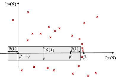
Figure 1: The location of complex zeros of the partition function, the critical point $\beta_{c}$, and the zero-free region near the real axis (as in Definition 2). The free energy is analytic in this region.

1.1.2 The decay of correlations in the Gibbs state

Another signature of the thermal phase transition is the appearance of long-range order in the system. In the example of a magnetic system, below the phase transition in the ferromagnetic phase (also called the ordered phase), distant spins are correlated and point in the same direction, whereas in the paramagnetic phase (also known as the disordered phase), the correlations between disjoint parts of the system decay exponentially with their distance. More precisely, we define the exponential decay of correlations as

Definition 5 (Informal version of Condition 2).

The Gibbs state $\rho_{\beta}(H)$ of a geometrically-local Hamiltonian $H$ at inverse temperature $\beta$ exhibits an exponential decay of correlations if for any two disjoint observables $O_{1}$ and $O_{2}$ there exist constants $\xi$ and $c$ such that

$$\big{|}\operatorname{tr}\left[\rho_{\beta}(H)O_{1}O_{2}\right]-\operatorname{tr}\left[\rho_{\beta}(H)O_{1}\right]\operatorname{tr}\left[\rho_{\beta}(H)O_{2}\right]\big{|}\leq c{||O_{1}||}{||O_{2}||}e^{-\mathrm{dist}(O_{1},O_{2})/\xi}.$$ (1)

Besides its physical significance, this property also has algorithmic applications and has been studied both in classical [Wei06] and quantum [KGK⁺14, BK16] settings. What is the relation between this notion of the phase transition and the complex zeros of the partition function? Note that the former involves correlations in the system at a real temperature while the latter concerns the complex temperature features of the partition function. Could it be that these two apparently distinct characterizations are indeed equivalent?

In a seminal work [DS87], Dobrushin and Shlosman proved that for translationally-invariant classical systems, the decay of correlations is actually equivalent to the analyticity of the free energy and the existence of a zero-free region. Recently, a more refined version of this equivalence was proved for the classical Ising model [LSS19a].

The same question has been open for quantum systems. Our next two results suggest an affirmative answer. Our first result shows that the absence of complex zeros around some real $\beta$ implies the exponential decay of correlations at that $\beta$.

Theorem 6 (Informal version of results in Section 5).

Let $\rho_{\beta}(H)$ be the Gibbs state of a geometrically-local Hamiltonian at inverse temperature $\beta$ in the zero-free region $\Omega_{\delta,\beta}$ given in Definition 2. This state has the decay of correlation property as in Definition 5 in any of the following cases:

• The distance between the observables $O_{1}$ and $O_{2}$ is at least $\Omega(\log n)$,

• The Hamiltonian $H$ is the sum of mutually commuting local terms, or

• The Hamiltonian $H$ is defined on a $1$D chain.

The class of commuting Hamiltonians include important examples such as stabilizer Hamiltonians like the Toric code, Color code, or Levin-Wen model [LW05].

Proving the converse of Theorem 6 turns out to be more challenging. Nevertheless, we can give evidence for this direction by generalizing the result of [DS87] to classical systems that are not translationally invariant, and also quantizing certain steps in the proof.

Theorem 7 (Informal version of Theorem 35).

Let $H$ be a geometrically-local Hamiltonian of a classical spin system, i.e. the local terms $H_{i}$ are all diagonal in the same product basis. For this system, the exponential decay of correlations given in Definition 5 implies the absence of zeros near the real axis as in Definition 2.

The importance of fully establishing this equivalence between the decay of correlations and the absence of zeros is twofold. On one hand, this can be thought of as an improvement on Theorem 4. This means we can prove the analyticity of the free energy not only below the lower bound $\beta_{0}$ that we found, which might be smaller than the exact value $\beta_{c}$, but also for any $\beta$ at which the decay of correlations holds. On the other hand, this equivalence allows us to use the locus of zeros to extend the range of $\beta$ where the system exhibits the decay of correlations from a constant (by a result of [KGK⁺14]) to the critical point $\beta_{c}$. Overall, this equivalence rigorously confirms the physical intuition that a quantum system enters the disordered phase at the point where the free energy becomes analytic.

1.1.3 Two-local Hamiltonians and Lee-Yang zeros

For our last result, we switch gears and focus on a specific family of $2$-local Hamiltonians. We again use the idea of extrapolation, but this time, our extrapolation parameter instead of $\beta$ is the strength of the external magnetic field applied to the system in the $z$-direction. The physical motivation is that when the system is subject to a large external field in a specific direction (the $z$-direction in our case), all spins align themselves in that direction, and estimating the properties of the system becomes trivial. On the other hand, as we move to smaller fields, the other interaction terms between the particles gain significance, making the problem non-trivial. Our result is an approximation algorithm for the quantum $\mathrm{XXZ}$ model with the following Hamiltonian:

Definition 8.

The anisotropic $\mathrm{XXZ}$ Hamiltonian on an interaction graph $G=(V,E)$ is given by

$$H(\mu)=-\sum_{(i,j)\in E}\left(J_{ij}(X_{i}X_{j}+Y_{i}Y_{j})+J_{ij}^{zz}Z_{i}Z_{j}\right)-\mu\sum_{i\in V}Z_{i}.$$ (2)

We find an approximation algorithm for this model. This is stated in the following theorem.

Theorem 9 (Informal version of Theorem 50).

There is a deterministic algorithm that runs in $n^{O(\log(n/\varepsilon))}$ time and outputs an $\varepsilon$-multiplicative approximation to the partition function of the anisotropic $\mathrm{XXZ}$ model (see Definition 8) in the ferromagnetic regime, i.e. when $J_{ij}^{zz}\geq|J_{ij}|$, and $\mu$ is an arbitrary constant.

1.2 Sketch of our techniques

Sketch of the proof for Theorem 3

The basis of our algorithm in Theorem 3 is the following observation. It is computationally easy to find the partition function and its derivatives at $\beta=0$. Note that in a system of $n$ qudits, $Z_{\beta=0}(H)=d^{n}$ and its derivatives are

$$\frac{d^{k}Z_{\beta}(H)}{d\beta^{k}}\Bigr{|}_{\beta=0}=(-1)^{k}\operatorname{tr}[H^{k}].$$ (3)

Since the local Hamiltonian $H$ equals $\sum_{i=1}^{m}H_{i}$ for some $m=\operatorname{poly}(n)$, its $k$th power $H^{k}$ is also the sum of $n^{O(k)}$ many local terms, i.e.

$$H^{k}=\sum_{j=1}^{n^{O(k)}}H^{(k)}_{j},$$ (4)

where $H^{(k)}_{j}$ is a product of $k$ local terms $H_{i}$. Each of the new terms $H^{(k)}_{j}$ acts on a region that is at most $k$ times larger than the support of the original terms $H_{i}$ which is still some constant. We can find $\operatorname{tr}[H^{k}]$ by adding $n^{O(k)}$ many terms like $\operatorname{tr}[H^{(k)}_{j}]$, which allows us to compute the derivatives (3) in time bounded by $n^{O(k)}$.

How can the solution at $\beta=0$ be used to estimate the one at some non-zero $\beta$? We use a technique due to Barvinok [Bar16b, Bar15] that has been applied to similar counting problems. The idea is to extrapolate this solution at $\beta=0$ to find $Z_{\beta}(H)$ at some non-zero $\beta$ where the problem is non-trivial. The extrapolation is done simply by using a truncated Taylor expansion of $\log Z_{\beta}(H)$ at $\beta=0$. Since our goal is to find the partition function with some $\varepsilon$-multiplicative error, it is sufficient to estimate $\log Z_{\beta}(H)$ within $\varepsilon$-additive error.

The main barrier to the reliability of this algorithm is establishing the fast convergence of the Taylor expansion. Such a Taylor expansion is only valid when $\log Z_{\beta}(H)$ remains a complex-analytic function, meaning the extrapolation is done along a path contained in the zero-free region. This is precisely the condition stated in Definition 2. Under this assumption, the Taylor theorem along with the bound $|\log Z_{\beta}(H)|\leq O(n)$ that we get from being in the zero-free region give

$$\left|\log Z_{\beta}(H)-\sum_{k=0}^{K-1}\frac{1}{k!}\frac{d^{k}\log Z_{\beta}(H)}{d\beta^{k}}\Bigr{|}_{\beta=0}\right|\leq c_{1}ne^{-c_{2}K}$$ (5)

for some constants $c_{1},c_{2}$ (see Proposition 18 in the body for details). The running time of computing the terms in this expansion is dominated by that of finding the derivatives which, as mentioned earlier, takes time $n^{O(K)}$. To get an additive error of $\varepsilon$ for $\log Z_{\beta}(H)$, it suffices to choose $K=O(\log(n/\varepsilon))$ resulting in a quasi-polynomial time algorithm.

The running time of this algorithm depends exponentially on the distance between the zeros and the extrapolation path. This allows us to clearly see why our algorithm fails beyond the phase transition point. If we try to extrapolate to $\beta\geq\beta_{c}$, we need to find a zero-free region that avoids the “armor” of zeros that are concentrated around the real axis at $\beta_{c}$. This results in a zero-free region with a vanishing width. Hence, the running time blows up, which matches our expectation from the ${\sf{NP}}$ hardness result above $\beta_{c}$ [SS12].

Sketch of the proof for Theorem 6

The technique used in the proof of Theorem 6 is inspired by the extrapolation idea of Theorem 3 and also the proof of the similar statement for the classical systems due to [DS87].

For any given disjoint observables $O_{1}$ and $O_{2}$, we define a function $f(\beta)$ that measures the correlation between them. This function is defined in a slightly different way than the covariance form in (1) and is tuned to have specific properties. In particular, we show that at $\beta=0$, the value of this function is zero, i.e. $f(0)=0$. This is expected intuitively since the system is in the maximally mixed state at $\beta=0$ and particles are distributed independently at random. However, we further show that the low order derivatives of this function up to $O(\mathrm{dist}(O_{1},O_{2}))$ are all zero at $\beta=0$, i.e.

$$\frac{d^{k}f(\beta)}{d\beta^{k}}\Bigr{|}_{\beta=0}=0,\quad\text{for\ }k=0,1,\dots,O(\mathrm{dist}(O_{1},O_{2})).$$ (6)

Hence, this function looks very flat around the origin. Additionally, we prove that $f(\beta)$ is an analytic function in the zero-free region. Finally, we show that this together with the constraints on the derivatives imply that the value of $f(\beta)$, which shows how correlated $O_{1}$ and $O_{2}$ are, remains exponentially small when moving from the origin to a constant $\beta$.

This gives us an upper bound $\propto n\exp(-\mathrm{dist}(O_{1},O_{2})/\xi)$ on the amount of correlation. The extra factor of $n$ makes this bound exponentially small when $\mathrm{dist}(O_{1},O_{2})=\Omega(\log n)$.

Remark 10.

Even with the extra factor of $n$, our bound remains useful for algorithmic applications such as in [BK16]. There one needs to split the system into computationally tractable smaller pieces and solve the problem for those pieces locally. The error of this strategy can be bounded using the exponential decay of correlations. To keep this error less than $1/\operatorname{poly}(n)$, one needs to choose the distances to be $O(\log n)$ which is the regime that our result covers.

We are able to remove the constraint $\mathrm{dist}(O_{1},O_{2})=\Omega(\log n)$ in certain instances. This includes when the Hamiltonian consists of commuting terms or when it is defined on a $1$D chain. In both cases, using either the commutativity of local terms or the quantum belief propagation [Has07] (refer to Proposition 14 in the body for the precise statement), we show that by removing the interaction terms acting on particles that are far from the observables $O_{1}$ and $O_{2}$, the correlations between $O_{1}$ and $O_{2}$ do not change by much. Hence, the system size reduces to the number of particles in the vicinity of the two observables. This number replaces the prefactor $n$ we had before and is negligible compared to the exponential factor $\exp(-\mathrm{dist}(O_{1},O_{2})/\xi)$. Thus, for these systems, the decay of correlations holds even when $\mathrm{dist}(O_{1},O_{2})$ is a constant.

Sketch of the proofs for Theorem 4 and Theorem 7

We first introduce a core idea which plays a central role in the proofs of both Theorem 20 and Theorem 6. For ease of notation, we denote the partition function of a geometrically-local Hamiltonian $H$ defined over a $D$-dimensional lattice $\Lambda\subset\mathbb{Z}^{D}$ by $Z_{\beta}(\Lambda)$. The particles are located on the vertices of this lattice.

In Theorem 4, our goal is to show that $Z_{\beta}(\Lambda)\neq 0$ inside a disk of radius $\beta_{0}$, i.e. for $\beta\in\mathbb{C}$ where $|\beta|\leq\beta_{0}$ for some constant $\beta_{0}$. We consider a series of sublattices $\emptyset=\Lambda_{0}\subset\Lambda_{1}\subset\Lambda_{2}\subset\dots\subset\Lambda_{n}=\Lambda$ such that each sublattice $\Lambda_{i}$ has one fewer vertex than $\Lambda_{i+1}$. By convention, we let $Z_{\beta}(\emptyset)=1$. As long as the sublattice $\Lambda_{i}$ has only a constant number of particles, we can always ensure $Z_{\beta}(\Lambda_{i})\neq 0$ by choosing $\beta$ to be a sufficiently small constant. One might worry that by adding more particles, the partition function vanishes. Our main contribution is to prove this does not happen. We do so by showing that the partition function after involving new particles cannot become smaller than a constant fraction of the partition function before adding the particles. In other words, we show there exists a constant $c>1$ such that

$$|Z_{\beta}(\Lambda_{i+1})|\geq c^{-1}|Z_{\beta}(\Lambda_{i})|,\quad i\in\{1,2,\dots,n-1\}.$$ (7)

By repeatedly applying this bound, we obtain the following exponentially small (yet sufficiently large for our purposes) lower bound on the partition function of the whole system

$$|Z_{\beta}(\Lambda)|\geq c^{-n}|Z_{\beta}(\Lambda_{1})|.$$ (8)

This leads to the bound given in Theorem 4. This lower bound is obtained using a method known as the cluster expansion. These expansions are widely used in statistical physics to study the high temperature behavior of classical and quantum many-body systems. The cluster expansion we use is due to Hastings [Has06, KGK⁺14], which represents the operator $\exp(H)$ as sum of products of local terms $H_{i}$. This allows us to express $Z_{\beta}(\Lambda_{i+1})$ in terms of $Z_{\beta}(\Lambda_{i})$ plus some small correction terms that account for the interaction terms acting on the added particle. Our main contribution is to use an inductive proof to connect such a decomposition to the lower bound (7) (see the proof of Theorem 20 in the body for details).

A similar strategy is used in the proof of Theorem 7 which closely follows the proof of the same statement for translationally-invariant systems in [DS87]. We essentially show a similar bound to (7) on how much the partition function can shrink after adding new particles. Here, instead of cluster expansions, we use the exponential decay of correlations to show such a lower bound. However, notice that the decay of correlations is a property of the system at a real $\beta$, whereas we want to bound the absolute value of the partition function at some complex $\beta$. There are multiple steps in the proof before we can get around this issue.

One crucial step is to reduce the proof of the analyticity of the free energy to a condition that roughly speaking (see Proposition 37 for the details) states that changing the value of a spin in the system only causes a small relative change in the partition function of the system even for complex $\beta$. We prove this by isolating the effect of this spin flip from the rest of the system using the decay of correlations. This requires removing the imaginary part of $\beta$ for all the interactions in the vicinity of the flipped spin and bounding the resulting error.

This overall approach involves a subtle use of the boundary conditions in the spin system. In the quantum case, this means applying local projectors to the Gibbs state before evaluating the partition function. These projectors can in general be entangled which makes using this proof technique more challenging for quantum systems.

Sketch of the proof for Theorem 9

Thus far we have only considered complex zeros of the partition function as a function of $\beta$. These are often called Fisher zeros [Fis65]. One can, however, fix $\beta$ and consider the partition function as a function of other parameters in the Hamiltonian. When that parameter is the strength of the external magnetic field denoted by $\mu$, these zeros are called Lee-Yang zeros [LY52]. In a pioneering result, Lee and Yang showed that for ferromagnetic systems, the locus of these zeros can be exactly determined and they are all on the imaginary axis in the complex $\mu$-plane.

A generalization of this theorem has been proved for a class of $2$-local quantum systems including the anisotropic Heisenberg model [SF71]. The result follows by mapping the quantum system to a classical spin system and applying a Lee-Yang type argument to the classical model.

Knowing the location of the complex zeros, we use the extrapolation algorithm to estimate the solution at a constant $\mu$ by finding the low-order derivatives of the partition function at $\mu=0$. We can apply this to the quantum $\mathrm{XXZ}$ model given in (2).

1.3 Previous work

1.3.1 Classical statistical physics and combinatorial counting

The Gibbs distribution and partition function appear naturally in combinatorial optimization, statistical physics, and machine learning. In particular, the classical Ising model has been studied extensively within these areas. These studies have cultivated in various probabilistic and deterministic approximation algorithms for this model and its variants. In the following, we summarize some of these results.

Most notable and the first rigorously proven efficient algorithm for the Ising model is the result of Jerrum and Sinclair [JS93] that uses a Markov chain Monte Carlo (MCMC) sampling algorithm to estimate the partition function in the ferromagnetic regime on arbitrary graphs. More generally, it has been shown that one can set up Markov chains for sampling from the Gibbs distribution that mix rapidly if and only if the correlations decay exponentially. This is known as the equivalence of mixing in time and mixing in space [Wei04] .

Another approach uses the decay of correlations in the Gibbs distribution. This property essentially allows one to decompose the interaction graph of the system into smaller computationally tractable pieces, and then combine the results of the computation on those pieces to find the overall partition function. In contrast to the MCMC approach, algorithms based on the decay of correlations can be deterministic – even in the regime where no MCMC algorithm is known. This approach, for instance, has lead to efficient deterministic algorithms for the hard-core model up to the hardness threshold [Wei06] and the antiferromagnetic Ising model [SST14].

There is a recent conceptually different approach to estimating the partition function, which is the basis of this work. This approach views the partition function as a high-dimensional polynomial and uses the truncated Taylor expansion to extend the solution at a computationally easy point to a non-trivial regime of parameters. Since its introduction [Bar16a], this method has been used to obtain deterministic algorithms for various interesting problems such as the ferromagnetic and antiferromagnetic Ising models [LSS19b, PR18] on bounded graphs.

As mentioned before, the equivalence of the analyticity of the free energy and the decay of correlations was first proved by Dobrushin and Shlosman [DS87]. The Fisher zeros of the classical Ising model and their relation to the correlation decay was also recently studied in [LSS19a].

1.3.2 Quantum many-body systems

The problem of estimating the partition function and correlation decay in quantum systems has also been studied in the past. We review some of these results here.

There are various results (e.g., [PW09, CS17]) that estimate the partition function by sampling from the Gibbs state using a quantum computer (also known as quantum Gibbs sampling). The best known bound on the running time of these algorithms is exponential in the number of particles. This running time can be reduced if we assume other conditions. For example, [KBa16] shows that a strong form of the decay of correlations implies an efficient quantum Gibbs sampler for commuting Hamiltonians. If in addition to the decay of correlations, we add the decay of quantum conditional mutual information, then this result can be extended to non-commuting Hamiltonians [BK16]. Turning these quantum algorithms into classical ones results in an $n^{\operatorname{polylog}(n)}$ running time. Although we cannot directly compare these results with our algorithm due to different conditions that are imposed, the $n^{O(\log n)}$ running time that we achieve outperforms that of these algorithms.

Considering the success of approximation schemes for the classical statistical problems, it is desirable to import those results to evaluate the thermal properties of interacting quantum many-body systems. This indeed can be done for some models like the quantum transverse field Ising model [Bra15] or the quantum $\mathrm{XY}$ model [BG17] in the ferromagnetic regime using what is called the quantum-to-classical mapping.

Establishing the decay of correlations in the Gibbs state has also been studied in quantum settings. In particular, it has been shown that the Gibbs state has this property in the $1$D translationally invariant case [Ara69] or above some constant temperature in higher dimensions [KGK⁺14]. Thus, in these regimes, there exist efficient representations for the state of the system using a tensor network ansatz like matrix product states or projected entanglement pair states [Has06, KGK⁺14, MSVC15]. However, this does not necessarily imply an efficient algorithm that finds and faithfully manipulates these tensor networks.

The decay of conditional mutual information is another property of the Gibbs state that has been rigorously proved for $1$D systems [KBa19] and conjectured for higher dimensions. This result has been used to find algorithmic schemes for preparing the Gibbs state on a quantum computer [BK16] or estimating the free energy in $1$D [Kim17, KS18]. A recent result of [KKB19] uses cluster expansions along with a technique very similar to the one we use in Theorem 6 (i.e. showing the low-order derivatives of the correlation function are zero) to establish the decay of conditional mutual information above some constant temperature.

1.4 Discussion and open questions

Our work raises many questions that we leave for future work. Here we mention some of them.

1. Perhaps the most immediate problem is to fully establish (or refute) the connection between the decay of correlations and the absence of zeros. There are at least two directions to pursue.

   1. It would be interesting to prove the exponential decay of correlations in the zero-free region of non-commuting Hamiltonians in higher dimensions. Currently we can only show this when the distance of the observables is $\Omega(\log n)$. It seems for this to work, the region of applicability of certain tools such as the quantum belief propagation needs to be extended to the complex regime.

   2. Establishing the absence of zeros in quantum systems when the correlations decay exponentially is also open. A first step might be to prove this for commuting Hamiltonians or $1$D chains. In Section 6, we have already extended some parts of the proof of this statement for the classical systems to commuting Hamiltonians, but it seems to complete the proof, a more careful analysis of the entangled boundary conditions is required.

2. While we focus on the covariance form of the correlations (1), one can also consider quantum conditional mutual information (qCMI) as a measure of correlations. Using the absence of zeros to prove the decay of qCMI is another interesting question. This would extend the result of [KKB19] to lower temperatures down to the phase transition point. Since the approach of [KKB19] resembles some of the techniques we use, this looks like a promising direction.

3. Is there some range of temperatures or Hamiltonian parameters that a quantum computer cannot efficiently sample from the Gibbs state but the extrapolation technique still works? At least, when the parameter of interest is temperature, this depends on the fate of the previous questions we mentioned, i.e. showing that the decay of correlations and qCMI are necessary for the absence of zeros. The result of [BK16] implies an efficient quantum sampler under the same conditions. Are there other parameters besides temperature for which one can show a separation between these notions?

4. Is it possible to improve the lower bound we obtained for the critical point $\beta_{c}$ in Theorem 4 without using other conditions such as the decay of correlations? In general, what is the computational hardness of determining the thermal phase transition point $\beta_{c}$?

5. Can the running time of our algorithm be improved for specific systems to polynomial time? This has been achieved for the classical Ising model [LSS19b, PR18] by relating the derivatives of the partition function to combinatorial objects that can be efficiently counted.

6. Can we use the extrapolation idea to avoid the sign problem? The easy regime, which includes the starting point of the extrapolation, could be a regime of parameters where the Hamiltonian is sign-free and MCMC algorithms yield a good estimate, whereas the end point is where the sign problem exists. A candidate parameter for extrapolation is the chemical potential. There are important physical systems such as lattice gauge theories for which at zero chemical potential the partition function is sign-free while there is a severe sign problem for non-zero chemical potentials.

7. Barvinok’s approach has been used to obtain approximation algorithms for other problems related to quantum computing [EM17, MB18, BGM19]. Are there other relevent applications for this method?

2 Preliminaries and notation

2.1 Local and geometrically-local Hamiltonians

Consider a $D$-dimensional lattice $\Lambda\subset\mathbb{Z}^{D}$ containing $n$ sites with a $d$-dimensional particle (qudit) on each site. The Hilbert space is ${\cal H}=\bigotimes_{i\in\Lambda}{\cal H}_{i}$ where ${\cal H}_{i}$ is the local Hilbert space of site $i$. For a region $A\subseteq\Lambda$, we denote its size by $|A|$ and its complement by $\bar{A}$. The diameter of $A$ is defined to be $\operatorname{diam}(A)=\sup\{\mathrm{dist}(x,y)\mathrel{\mathop{\mathchar 58\relax}}x,y\in A\}$. The interaction of these particles is described by a local Hamiltonian $H$ that has the following form:

$$H=\sum_{X\subset\Lambda}H_{X}.$$ (9)

Each term $H_{X}$ is a Hermitian operator with operator norm at most $h$ that is acting non-trivially only on the sites in $X$. We denote this by writing $\operatorname{supp}(H_{X})=X$. The local terms $H_{X}$ do not necessarily commute with each other. Similarly, we define $H_{A}=\sum_{X\subseteq A}H_{X}$ to be the Hamiltonian restricted to a region $A\subseteq\Lambda$. We denote the number of local terms in the Hamiltonian by $m$ and often also write $H=\sum_{i=1}^{m}H_{i}$. The $1$-norm of an operator $O$ is denoted by ${||O||}_{1}$ and its operator norm by ${||O||}$.

In order to impose geometric locality on the interactions between the particles, we consider the interactions that satisfy the following condition.

Definition 11 (Geometrically-local Hamiltonians).

A Hamiltonian $H=\sum_{X\subset\Lambda}H_{X}$ such that $\operatorname{supp}(H_{X})=0$ when $\operatorname{diam}(X)>R$ or $|X|>\kappa$ is called a $(\kappa,R)$-local Hamiltonian. We call $\kappa$ the locality and $R$ the range of $H$. We use the words geometrically-local and $(\kappa,R)$-local interchangeably when $\kappa,R$ are kept constant.

This should be contrasted with the case where $\operatorname{supp}(H_{X})=0$ when $|X|>\kappa$ but there is no restriction on $\operatorname{diam}(X)$. In order to distinguish between these two, we use the terms geometrically-local versus local throughout this paper. We also focus mostly on geometrically-local Hamiltonians with a finite range $R$, but most of our results also apply to Hamiltonians with interactions that decay fast enough, for example, with some exponential rate.

Remark 12.

In general, the locality $\kappa$ of a geometrically-local Hamiltonian on a $D$-dimensional lattice $\Lambda$ can be bounded as $\kappa\leq O(D^{R})$, which is the size of a ball of diameter $R$. Nevertheless, we treat both $\kappa$ and $R$ as independent parameters in this paper.

For the Hamiltonians we consider, the sum $|\sum_{X\cap\{x_{0}\}\neq\emptyset}H_{X}|$ is bounded from above by a constant like $O(hD^{\kappa R})$, but in general, this is a loose bound and we introduce the growth constant as an independent parameter such that:

Definition 13 (Growth constant).

Given a geometrically-local Hamiltonian $H$, the growth constant $g$ is defined such that $|\sum_{X\cap\{x_{0}\}\neq\emptyset}H_{X}|\leq gh$ for all sites $x_{0}\in\Lambda$.

Given a $(\kappa,R)$-local Hamiltonian $H$, we denote the boundary of a region $A\subseteq\Lambda$ by $\partial A$ and define it as $\partial A=\{v\in\Lambda\setminus A\mathrel{\mathop{\mathchar 58\relax}}\exists v^{\prime}\in A,\ \mathrm{dist}(v-v^{\prime})\leq R\}$. Defined this way, the boundary of $A$ is a subset of $\bar{A}$.

For local Hamiltonians with $\kappa=2$, we define an interaction graph which is an undirected graph $G=(V,E)$ with a qudit on each vertex $v\in V$ and an edge $(i,j)$ between any two vertices $i,j$ that are acted on by a local term in the Hamiltonian. For qubits, $d=2$ and such a Hamiltonian is of the following form:

$$H=-\sum_{\begin{subarray}{c}(i,j)\in E\\ a,b\in\{x,y,z\}\end{subarray}}J_{ij}^{ab}\sigma_{a}\otimes\sigma_{b}-\sum_{\begin{subarray}{c}i\in V\\ a\in\{x,y,z\}\end{subarray}}h^{a}_{i}\sigma_{a},$$ (10)

where $J_{ij}^{ab},h_{i}^{a}\in\mathbb{R}$ are the interaction coefficients and $\sigma_{a}\in\{X,Y,Z,\mathds{1}\}$ are Pauli matrices.

2.2 Quantum thermal state and partition function

The free energy of state $\rho$ at inverse temperature $\beta$ is defined as

$$F_{\beta}(\rho)=\operatorname{tr}(H\rho)-\frac{1}{\beta}S(\rho),$$

where $S(\rho)=-\operatorname{tr}(\rho\log\rho)$ is the von Neumann entropy of $\rho$ (here and throughout this paper, we assume $\log$ denotes the natural logarithm). In thermal equilibrium, the free energy of the system is minimized. Using the non-negativity of the relative entropy $S(\rho\|\frac{e^{-\beta H}}{Z(\beta)})\geq 0$, one can see that

$$\min_{\rho}F_{\beta}(\rho) =\min_{\rho}\operatorname{tr}(H\rho)-\frac{1}{\beta}S(\rho)$$ (11)

$$=-\frac{1}{\beta}\log(Z_{\beta}(\Lambda)),$$

where $Z_{\beta}(H)=\operatorname{tr}[\exp(-\beta H)]$ is the partition function of the system at inverse temperature $\beta$. When dealing with spin systems on a lattice, we often denote the partition function of the system by $Z_{\beta}(\Lambda)$ rather than $Z_{\beta}(H)$.

Furthermore, the state that achieves this minimization, known as the Gibbs (or thermal) state, is given by

$$\rho_{\beta}(H)=\frac{\exp(-\beta H)}{Z_{\beta}(H)}.$$ (12)

We often need to consider the Gibbs state after some measurement has been performed on a local region of the lattice. The post-selected state $\rho_{\beta}(H|N)$ associated with a positive operator $N$ is given by

$$\rho_{\beta}(H|N)=\frac{\sqrt{N}\exp(-\beta H)\sqrt{N}}{\operatorname{tr}[\exp(-\beta H)N]}.$$ (13)

2.3 Quantum belief propagation

Suppose certain local terms in Hamiltonian $H$ are removed and consider the Gibbs state before and after this change. We would like to relate these Gibbs states by applying a local operator on the old state to obtain the new one. This has been addressed before in [Has07] under the name quantum belief propagation. We only mention this result without the proof and refer the reader to [Has07, KBa19] for the derivation and more details.

Proposition 14 (Quantum belief propagation).

Let $H$ be a geometrically-local Hamiltonian on lattice $\Lambda$. Consider a sublattice $C\subset\Lambda$. We denote the terms in $H$ acting on both $C$ and $\bar{C}$ by $H_{\partial C}$. There exists a quasi-local operator $\eta$ such that

$$e^{-\beta H}=\eta e^{-\beta(H-H_{\partial C})}\eta^{{\dagger}},$$ (14)

where ${||\eta||}\leq\exp(\beta/2{||H_{\partial C}||})$. Moreover, there exists a truncation of $\eta$ denoted by $\eta_{\ell}$ supported non-trivially only on $\partial C$ and sites within distance $\ell$ from $\partial C$ such that for some positive constants $\alpha_{1},\alpha_{2}$,

$${\big{|}\big{|}\eta-\eta_{\ell}\big{|}\big{|}}\leq e^{\alpha_{1}|\partial C|-\alpha_{2}\ell}.$$ (15)

2.4 Tools from complex analysis

Given a function that is analytic in a region of the complex plane, i.e. it is complex differentiable, we are interested in approximating the function in that region with a low-degree polynomial. Conventional methods in complex analysis allow us to achieve this using a Taylor expansion around a point inside that region.

Definition 15 (Taylor expansion of analytical functions).

Given a complex function $f(z)$ that is analytic in a region $A$, the Taylor expansion of $f(z)$ around a point $z_{0}\in A$ is a power series $\sum_{k=0}^{\infty}a_{k}(z-z_{0})^{k}$, where for $\forall k=0,1,\dots$

$$a_{k}=\frac{1}{k!}\frac{d^{k}f(z_{0})}{dz^{k}}=\frac{1}{2\pi i}\oint_{C}\frac{f(w)}{(w-z_{0})^{k+1}}dw$$ (16)

for an arbitrary contour $C$ around $z_{0}$ inside the region $A$.

In Section 7, we map the partition function of a quantum system to that of a classical system. As we increase the precision of the mapping, we get a family of classical systems with increasing size that in the limit of an infinite number of particles have the same partition function as the quantum system. The following theorem guarantees that the zero-free region of the classical ensemble coincides with that of the original quantum system.

Theorem 16 (Multivariate Hurwitz’s theorem).

If a sequence of multivariate functions $f_{1},f_{2},f_{3},\dots$ are analytic and non-vanishing on a connected open set $D\subset\mathbb{C}^{n}$ and converge uniformly on compact subsets of $D$ to $f$, then f is either non-vanishing on $D$ or is identically zero.

The proof can be found in standard complex analysis textbooks [Gam03].

3 Algorithm for estimating the partition function

In this section, we provide more details about the approximation algorithm that we presented in Section 1.

Definition 17.

An approximation algorithm for the partition function $Z_{\beta}(H)$ takes as input the description of the local Hamiltonian $H$, the inverse temperature $\beta$, and a parameter $\varepsilon$ and gives an estimate $\tilde{Z}_{\beta}(H)$ with $\varepsilon$-multiplicative error, i.e.

$$\left|\tilde{Z}_{\beta}(H)-Z_{\beta}(H)\right|\leq\varepsilon Z_{\beta}(H).$$ (17)

This is, up to unimportant constants, equivalent to finding an $\varepsilon$-additive error for $\log Z_{\beta}(H)$ or $F_{\beta}(H)$.

We now make a connection between analyticity of functions and approximation algorithms precise. Similar propositions were first proved by [Bar16a] for bounded degree polynomials.

Suppose we want to estimate the value of a complex function $f(z)$. We consider two cases. One is when there is an upper bound on the absolute value of the function in the region that $f(z)$ is analytic. The other is when the given function is $f(z)=\log(g(z))$ for a polynomial $g(z)$ of degree $n$. The latter is used in Section 7.2 when studying the $\mathrm{XXZ}$ model. We need the former version since as we will see in Theorem 19, the partition function of quantum (or even some classical) systems is not always a polynomial in $\beta$.

Proposition 18 (Truncated Taylor series for bounded functions and polynomials).

We denote a disk of radius $b$ centered at the origin in the complex plane by $\Delta_{b}$, that is $\Delta_{b}=\{z\in\mathbb{C}\mathrel{\mathop{\mathchar 58\relax}}|z|\leq b\}$.

• Let $f(z)$ be a complex function that is analytic and bounded as $|f(z)|\leq M$ when $z\in\Delta_{b}$ for a constant $b>1$. Then the error of approximating $f(z)$ by a truncated Taylor series of order $K$ for all $|z|\leq 1$ is bounded by

  $$\left|f(z)-\sum_{k=0}^{K}a_{k}z^{k}\right|\leq\frac{M}{b^{K}(b-1)},\quad|z|\leq 1.$$ (18)

• Assume $b$ is fixed and there is a deterministic algorithm that finds the coefficients $a_{k}$ in time $O(N^{k})$ for some parameter $N$. Then there exists a deterministic algorithm with running time $N^{O(\log(M/\varepsilon))}$ that outputs an $\varepsilon$-additive approximation for $f(z)$.

• [cf. [Bar16a]] Let $f(z)=\log(g(z))$ for some polynomial $g(z)$ of degree $N$ that does not vanish when $z\in\Delta_{b}$. The error of approximating $f(z)$ by a truncated Taylor series of order $K$ for $|z|\leq 1$ is bounded by $\frac{N}{K+1}\frac{1}{b^{K}(b-1)}$.

• [cf. [Bar16a]] Assuming $b$ is fixed, there exists a deterministic algorithm with running time $N^{O(\log(N/\varepsilon))}$ that outputs an $\varepsilon$-additive approximation for $\log(g(z))$.

Proof.

The proof of (1) is a basic result in complex analysis based on the Cauchy integral theorem for analytic functions. Let $C^{\prime}$ be the circle $|z|=b$ that contains both $z$ and $z=0$. We have

$$f(z)= \frac{1}{2\pi i}\oint_{C^{\prime}}\frac{f(w)}{w-z}dw=\frac{1}{2\pi i}\oint_{C^{\prime}}\frac{f(w)}{w}\left(1-\frac{z}{w}\right)^{-1}dw$$

$$=\frac{1}{2\pi i}\oint_{C^{\prime}}\frac{f(w)}{w}\left(\sum_{k=0}^{K}\left(\frac{z}{w}\right)^{k}+\left(\frac{z}{w}\right)^{K+1}\left(1-\frac{z}{w}\right)^{-1}\right)dw$$

$$=\sum_{k=0}^{K}\frac{f^{(k)}(0)}{k!}z^{k}+\frac{1}{2\pi i}\oint_{C^{\prime}}\frac{f(w)}{w-z}\left(\frac{z}{w}\right)^{K+1}dw,$$

in which we used Eq. (16) to get to the last line. We can now bound the remainder as

$$\left|f(z)-\sum_{k=0}^{K}\frac{f^{(k)}(0)}{k!}z^{k}\right| \leq\frac{1}{2\pi}\oint_{C^{\prime}}\frac{|f(w)|}{|w-z|}\left(\left|\frac{z}{w}\right|\right)^{K+1}dw.$$

$$\leq M\frac{b}{b-1}\left(\frac{1}{b}\right)^{K+1},$$ (19)

where the last line follows from the fact that $|w-z|\geq b-1$, $|z|\leq 1$, and $|f(w)|\leq M$ on $C^{\prime}$.

The proof of part (3) is similar to that of (1). The degree $N$ polynomial $g(z)$ has at most $N$ complex roots $\{\zeta_{k}\}_{k=1}^{N}$ such that $|\zeta_{k}|\geq b$. Thus, $g(z)=g(0)\prod_{l=1}^{N}(1-\frac{z}{\zeta_{l}})$ and

$$\log(g(z))=\log(g(0))+\sum_{l=1}^{N}\log\left(1-\frac{z}{\zeta_{l}}\right),\quad\forall z\mathrel{\mathop{\mathchar 58\relax}}\ |z|\leq 1.$$ (20)

We can expand each term like $\log(1-\frac{z}{\zeta_{l}})$ as

$$\log\left(1-\frac{z}{\zeta_{l}}\right)=-\sum_{k=1}^{K}\frac{z^{k}}{k\zeta_{l}^{k}}+q_{\ell}(z),$$ (21)

where similar to part (1), we see that $q_{\ell}(z)$ is a term that can be bounded by

$$|q_{\ell}(z)|\leq\frac{1}{K+1}\frac{1}{b^{K}(b-1)}.$$ (22)

Hence, the remainder term in the Taylor expansion of $\log(g(z))$ up to order $K$ is $q(z)=\sum_{{\ell}=1}^{N}q_{\ell}(z)$, which is bounded by $|q(z)|\leq\frac{N}{K+1}\frac{1}{b^{K}(b-1)}$ as claimed in part (3).

In order to find the algorithms of part (2) and (4), we need to evaluate the Taylor coefficients of $f(z)$ up to some degree $K$. Since we want an $\varepsilon$-additive approximation of $f(z)$, one can see from parts (1) and (2) that it is sufficient to keep the Taylor expansion until order $K=O(\log(\frac{M}{\varepsilon}))$ for part (2) and $K=O(\log(\frac{N}{\varepsilon}))$ for part (4). To be able to evaluate the derivatives $\frac{d^{k}f(z)}{dz^{k}}$, we express them in terms of the derivatives of $g(z)$, i.e. $\frac{d^{k}g(z)}{dz^{k}}$ . This can be done by noticing that

$$\frac{d^{k}g(z)}{dz^{k}}=\sum_{\ell=0}^{k-1}\binom{k-1}{\ell}\frac{d^{\ell}g(z)}{dz^{\ell}}\frac{d^{k-\ell}f(z)}{dz^{k-\ell}},$$ (23)

so if we have access to $\frac{d^{k}g(z)}{dz^{k}}$, we can find $\frac{d^{k}f(z)}{dz^{k}}$ by solving the system of equations in time $\operatorname{poly}(k)$. The important step, however, is to estimate $\frac{d^{k}g(z)}{dz^{k}}$. This by assumption takes time $N^{O(k)}$ for the $k$th derivative. Thus, evaluating the Taylor expansion in parts (2) and (4) can be done in time $N^{O(\log(M/\varepsilon))}$ and $N^{O(\log(N/\varepsilon))}$, respectively.     $\sqcap$$\sqcup$

Theorem 19 (Extrapolation algorithm for estimating the partition function).

There exists a deterministic classical algorithm that runs in time $n^{O(\log(n/\varepsilon))}$ and outputs an estimate within $\varepsilon$-multiplicative error of the partition function $Z_{\beta}(H)$ at some constant $\beta$ in the zero-free region $\Omega_{\delta,\beta}$ (see Definition 2).

Proof of Theorem 19.

We apply the truncated Taylor expansion. To use that result, we first need to specify the zero-free region and then bound the running time of computing the $k$th derivative by $n^{O(k)}$.

We can without loss of generality assume that the zero-free region $\Omega_{\delta,\beta}$ is a rectangular region of constant width and size depicted in Figure 1. The result of Proposition 18, however, holds when the zero-free region is a disk of radius $b$. To match these domains, we can compose the partition function with a function $\phi(z)$ that maps a disk of radius $b$ to the rectangular region $\Omega_{\delta,\beta}$ such that $\phi(0)=0$ and $\phi(1)=\beta$ and $b$ is constant depending on $\delta$. It is shown in Lemma 2.2.3 of [Bar16a] that one can find such a $\phi(z)$ which is a constant degree polynomial. Hence, the composed partition function is non-zero and bounded on this disk and we can apply the bound (18) on the Taylor expansion.

As mentioned in Section 1.2, for a system of $n$ qudits, we can compute the order $k$ derivatives of $Z_{\beta}(H)$ in time $n^{O(k)}$. Similarly, we can evaluate the derivatives of $Z_{\beta}(H)$ composed with the constant-degree polynomial $\phi(z)$ using the same running time. Keeping only $k=O(\log(n/\varepsilon))$ many terms results in a quasi-polynomial algorithm with multiplicative error $\varepsilon$.     $\sqcap$$\sqcup$

4 Lower bound on the critical inverse temperature

In this section, we show that at high temperatures, there are no complex zeros near the real axis. More precisely, we prove that there exists a disk of constant radius $\beta_{0}$ centered at $\beta=0$ that does not contain any zeros and the free energy is analytic inside it. The radius $\beta_{0}$ depends only on the geometric parameters of the Hamiltonian such as the growth constant.

Theorem 20 (High temperature zeros).

Let $H$ be a gometrically-local Hamiltonian on qudits with range $R$, growth constant $g$, and local interactions with norm at most $h$ (see Definition 11 and Definition 13). There exists a real constant $\beta_{0}=1/(5egh\kappa)$ such that for all $\beta\in\mathbb{C}$ with $|\beta|\leq\beta_{0}$, the partition function $Z_{\beta}(\Lambda)$ of $H$ does not vanish and $\log(Z_{\beta}(\Lambda))$ is analytic and bounded by $\big{|}\log|Z_{\beta}(\Lambda)|\big{|}\leq(e^{2}gh|\beta|+\log d)n$.

This gives a lower bound $\beta_{0}\leq\beta_{c}$ on the phase transition point $\beta_{c}$. Also, as outlined in Theorem 19, if we can establish an upper bound like $\big{|}\log|Z_{\beta}(\Lambda)|\big{|}\leq O(n)$ for small enough complex $\beta$, we can devise an approximation algorithm for the partition function. Hence we get

Corollary 21 (Approximation algorithm for the partition function at high temperatures).

There exists a quasi-polynomial time algorithm with running time $n^{O(\log(n/\varepsilon))}$ that outputs an $\varepsilon$-multiplicative approximation to the partition function $Z_{\beta}(\Lambda)$ of a geometrically-local Hamiltonian $H$ when $|\beta|\leq\beta_{0}$.

Before getting to the proof of Theorem 20, we need to gather some facts and lemmas. Given a lattice $\Lambda\subset\mathbb{Z}^{D}$ with $n$ sites, we consider a series of sublattices $\Lambda_{0}\subset\Lambda_{1}\subset\Lambda_{2}\subset\Lambda_{2}\subset\dots\subset\Lambda_{n}=\Lambda$ such that each sublattice $\Lambda_{j}$ has one fewer vertex than $\Lambda_{j+1}$ and $\Lambda_{0}=\emptyset$. The partition function of $\Lambda_{0}$ is assigned to be $Z_{\beta}(\emptyset)=1$ for any complex $\beta$. Therefore, we can write

$$Z_{\beta}(\Lambda)=d^{n}\prod_{j=0}^{n-1}\left(\frac{1}{d}\frac{Z_{\beta}(\Lambda_{j+1})}{Z_{\beta}(\Lambda_{j})}\right),$$ (24)

where the factors of $d$ are added for later convenience and to account for the dimension of the removed sites. In order to show $\left|\log\left|Z_{\beta}(\Lambda)\right|\right|\leq O(n)$ for a $\beta\in\mathbb{C}$, we just need to bound the logarithm of each of the terms in Eq. (24) by a constant, i.e.

$$\left|\log\Big{|}\frac{1}{d}\frac{Z_{\beta}(\Lambda_{j+1})}{Z_{\beta}(\Lambda_{j})}\Big{|}\right|\leq O(1).$$ (25)

This bound tells us how much the partition function changes after removing a single site from the lattice. We later prove this by induction on the number of sites. However, as shown in the following lemma, this inequality is always satisfied when $\beta$ is real.

Lemma 22 (Site removal bound).

The following bound holds for any $X\subseteq\Lambda$ and $\beta\in\mathbb{R}^{+}$:

$$\left|\log\Big{|}\frac{1}{d^{|X|}}\frac{Z_{\beta}(\Lambda)}{Z_{\beta}(\Lambda\setminus X)}\Big{|}\right|\leq gh|\beta||X|.$$ (26)

Recall that $h$ is the maximum norm of the local terms $H_{X}$ in $H$ and the growth constant $g$ is chosen such that $|\sum_{X\cap\{x_{0}\}\neq\emptyset}H_{X}|\leq gh$ for all sites $x_{0}\in\Lambda$.

Proof.

We have

$$Z_{\beta}(\Lambda)=\operatorname{tr}_{\Lambda}\big{[}e^{-\beta(H_{\Lambda\setminus X}+\sum_{X^{\prime}\subset\Lambda\mathrel{\mathop{\mathchar 58\relax}}X^{\prime}\cap X\neq\emptyset}H_{X^{\prime}})}\big{]} \leq\operatorname{tr}_{\Lambda}\big{[}e^{-\beta H_{\Lambda\setminus X}}e^{-\beta\sum_{X^{\prime}\subset\Lambda\mathrel{\mathop{\mathchar 58\relax}}X^{\prime}\cap X\neq\emptyset}H_{X^{\prime}}}\big{]}$$

$$\leq\operatorname{tr}_{\Lambda}\big{[}e^{-\beta H_{\Lambda\setminus X}}\big{]}{\big{|}\big{|}e^{-\beta\sum_{X^{\prime}\subset\Lambda\mathrel{\mathop{\mathchar 58\relax}}X^{\prime}\cap X\neq\emptyset}H_{X^{\prime}}}\big{|}\big{|}}$$

$$\leq d^{|X|}\operatorname{tr}_{\Lambda\setminus X}\big{[}e^{-\beta H_{\Lambda\setminus X}}\big{]}e^{{\big{|}\big{|}\beta\sum_{X^{\prime}\subset\Lambda\mathrel{\mathop{\mathchar 58\relax}}X^{\prime}\cap X\neq\emptyset}H_{X^{\prime}}\big{|}\big{|}}}$$

$$\leq Z_{\beta}(\Lambda\setminus X)d^{|X|}e^{gh|\beta||X|},$$ (27)

where $H_{\Lambda\setminus X}$ corresponds to the terms in the Hamiltonian acting on the remaining sublattice $\Lambda\setminus X$. We used the Golden-Thompson inequality in the first line and the Hölder inequality to get to the second line. The factor $d^{|X|}$ is added since the original trace is over the Hilbert space of $\Lambda$ and not $\Lambda\setminus X$. Similarly, one can show $d^{|X|}Z_{\beta}(\Lambda\setminus X)\leq Z_{\beta}(\Lambda)e^{gh|\beta||X|}$. These bounds together prove the lemma.     $\sqcap$$\sqcup$

Theorem 20 extends bound (26) to the case where $\beta$ is a small complex number. We prove this in two steps.

First step:

In contrast to the proof of Lemma 22, the Golden-Thompson inequality can no longer be used in the complex regime. Hence, to compare the partition function before and after removing a site $x_{0}$, we need to find another way of separating the contribution of the terms in the Hamiltonian that act on $x_{0}$. We achieve this using a cluster expansion for the partition function that expands the operator $\exp(-\beta H)$ into a sum of products of local terms in $H$. The idea of using cluster expansions to study high temperature properties of classical or quantum spin systems has been widely applied before [KP86, Dob96, Par82, Gre69]. Here, we use a particular version of that expansion which is tailored for our application. This was first introduced in [Has06] and later improved and generalized in [KGK⁺14]. In Section 4.1, we modify the result of [Has06, KGK⁺14] and adapt it for complex partition functions.

Second step:

Our next step is to use the cluster expansion and show that in the partition function, the contribution of the sites acting on $x_{0}$ compared to the rest of the terms is bounded by a constant. We show this in Section 4.2 by induction on the number of sites. This is our main contribution and lets us prove the bound (26).

4.1 The cluster expansion for the partition function

When using the cluster expansion, we often need to consider products of local terms like $\prod_{j=1}^{\ell}H_{X_{j}}$, but since the local interaction terms $H_{X_{j}}$ do not necessarily commute with each other, we set an $\ell$-tuple $(X_{1},\dots,X_{\ell})$ to indicate the order of multiplication. We also need to decompose the sequence $(X_{1},\dots,X_{\ell})$ into the union of connected components. Let us define what we mean by connected more formally.

Definition 23 (Connected sets).

Fix a site $x_{0}\in\Lambda$. A collection of sublattices such as ${\cal X}=\{X_{1},X_{2},\dots,X_{k}\}$ is called a connected set containing $x_{0}$ with size $|{\cal X}|=k$ if the following conditions hold

• All the sublattices $X_{1},X_{2},\dots,X_{k}$ have bounded size and diameter. That is $1\leq|X_{i}|\leq\kappa$ and $\operatorname{diam}(X_{i})\leq R$.

• For any sublattice $X_{i}$ in ${\cal X}$, a series of other members of ${\cal X}$ connect this set to the site $x_{0}$. See Figure 2 for an example. More precisely we have: for any $X_{i}\in{\cal X}$, there exists $I\subseteq[k]$ such that $i\in I$ and $\forall j\in I,\exists\ell\in I\mathrel{\mathop{\mathchar 58\relax}}X_{j}\neq X_{\ell}$ yet $X_{j}\cap X_{l}\neq\emptyset$, and moreover, $x_{0}\in\cup_{j\in I}X_{j}$.

Although ${\cal X}$ consists of sublatices of $\Lambda$ and not individual sites, in a slight abuse of notation, we specify a set ${\cal X}$ that contains the site $x_{0}$ by $x_{0}\in{\cal X}$. We denote all the sites that a connected set ${\cal X}$ includes by $\operatorname{supp}({\cal X})$.

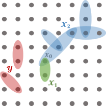
Figure 2: The sets ${\cal X}_{1},{\cal X}_{2}$ are connected, contain $x_{0}$, and have size $|{\cal X}_{1}|=1,|{\cal X}_{2}|=4$. However, the set ${\cal Y}$ is not connected, does not include $x_{0}$, and has size $|{\cal Y}|=2$.

Remark 24.

In Definition 23, we include an upper bound on the size and diameter of the subsets in ${\cal X}$, i.e. $|X_{i}|\leq\kappa,\operatorname{diam}(X_{i})\leq R$. This is because for geometrically-local Hamiltonians, ${||H_{X}||}=0$ for $|X_{i}|>\kappa,\ \operatorname{diam}(X_{i})>R$, so we do not need to consider those sets.

In the upcoming proofs, we need to have an upper bound on the number of the connected sets ${\cal X}$ that contains a specific site $x_{0}\in\Lambda$. This is stated in the following lemma.

Lemma 25 (Cf. [KGK⁺14]).

The number of connected sets ${\cal X}$ of size $|{\cal X}|$ containing the site $x_{0}\in\Lambda$ is upper bounded by $g^{|{\cal X}|}$ where $g$ is the growth constant of the Hamiltonian $H$ (see Definition 13). In particular, for a D-dimensional lattice and $\kappa=2$, we have $g\leq 2eD$.

The next lemma achieves the first step in our proof by setting up the cluster expansion for the partition function.

Lemma 26 (High temperature expansion).

For any $x_{0}\in\Lambda$, the partition function of the lattice $Z_{\beta}(\Lambda)$ admits the following decomposition for $|\beta|\leq\frac{1}{gh(e-1)}$:

$$Z_{\beta}(\Lambda)=d\cdot Z_{\beta}(\Lambda\setminus X_{0})+\sum_{\begin{subarray}{c}{\cal X}\mathrel{\mathop{\mathchar 58\relax}}x_{0}\in{\cal X}\\ {\cal X}\text{\ is connected\ }\end{subarray}}W_{\beta}({\cal X})Z_{\beta}(\Lambda\setminus\operatorname{supp}({\cal X})),$$ (28)

where $X_{0}=\{x_{0}\}$ and we define $W_{\beta}({\cal X})$ as

$$W_{\beta}({\cal X})=\sum_{p=|{\cal X}|}^{\infty}\frac{(-\beta)^{p}}{p!}\big{(}\sum_{\begin{subarray}{c}(X_{1},\dots,X_{p})\\ \forall i\in[p]\mathrel{\mathop{\mathchar 58\relax}}X_{i}\in{\cal X}\\ {\cal X}=\cup_{i=1}^{p}\{X_{i}\}\end{subarray}}\operatorname{tr}_{\operatorname{supp}({\cal X})}\big{[}\prod_{j=1}^{p}H_{X_{j}}\big{]}\big{)}.$$ (29)

The last sum in (29) is over all p-tuples $(X_{2},X_{2},\dots,X_{p})$ that one can form from members of ${\cal X}$ by repeating them at least once.

Proof.

We start by Taylor expanding $\exp(-\beta H)$. We have

$$Z_{\beta}(\Lambda) =\operatorname{tr}_{\Lambda}\big{[}\sum_{k=0}^{\infty}\frac{(-\beta)^{k}}{k!}(\sum_{X\subset\Lambda}H_{X})^{k}\big{]}$$

$$=\operatorname{tr}_{\Lambda}\big{[}\sum_{k=0}^{\infty}\frac{(-\beta)^{k}}{k!}(\sum_{X\subset\Lambda\setminus X_{0}}H_{X}+\sum_{X\subset\Lambda\mathrel{\mathop{\mathchar 58\relax}}X\cap X_{0}\neq\emptyset}H_{X})^{k}\big{]}$$

$$=\operatorname{tr}_{\Lambda}\big{[}\sum_{k=0}^{\infty}\frac{(-\beta)^{k}}{k!}(\sum_{X\subset\Lambda\setminus X_{0}}H_{X})^{k}\big{]}+\operatorname{tr}_{\Lambda}\big{[}\sum_{\ell=1}^{\infty}\frac{(-\beta)^{\ell}}{\ell!}\sum_{\begin{subarray}{c}(X_{1},\dots,X_{\ell})\\ \forall i\in[\ell]\mathrel{\mathop{\mathchar 58\relax}}X_{i}\subset\Lambda\\ \exists X_{i}\mathrel{\mathop{\mathchar 58\relax}}X_{i}\cap X_{0}\neq\emptyset\end{subarray}}\prod_{j=1}^{\ell}H_{X_{j}}\big{]},$$ (30)

where the trace is over the Hilbert space of $\Lambda$ as usual. The first term in the last line is just the Taylor expansion of $d\cdot Z_{\beta}(\Lambda\setminus X_{0})$. As in Eq. (27), the factor $d$ is included because the original trace is over $\Lambda$ and not $\Lambda\setminus X_{0}$. The last term, however, does not have a closed form, and involves summing over all the products of the local interaction terms $H_{X_{j}}$ such that at least one of the terms has non-empty overlap with the site $x_{0}$. We can simplify this term by partitioning the sequence $(X_{1},\dots,X_{l})$ into two parts. The first part forms a connected set ${\cal X}$ that contains the site $x_{0}$. The second part contains all $X_{i}$ that do not intersect with this connected set ${\cal X}$. We then change the order of the summation in (30) by first summing over all $X_{i}$ not connected to a fixed ${\cal X}$ and then varying the set ${\cal X}$. We get

$$\sum_{\ell=1}^{\infty}\frac{(-\beta)^{\ell}}{\ell!}\sum_{\begin{subarray}{c}(X_{1},\dots,X_{l})\\ \forall i\in[\ell]\mathrel{\mathop{\mathchar 58\relax}}X_{i}\subset\Lambda\\ \exists X_{i}\mathrel{\mathop{\mathchar 58\relax}}X_{i}\cap X_{0}\neq\emptyset\end{subarray}}\operatorname{tr}_{\Lambda}\big{[}\prod_{j=1}^{\ell}H_{X_{j}}\big{]}$$

$$=\sum_{p=|{\cal X}|,q=0}^{\infty}\binom{p+q}{p}\frac{(-\beta)^{p+q}}{(p+q)!}\sum_{\begin{subarray}{c}(X_{1},\dots,X_{p})\\ \forall i\in[p]\mathrel{\mathop{\mathchar 58\relax}}X_{i}\in{\cal X}\\ {\cal X}=\cup_{i=1}^{p}\{X_{i}\}\end{subarray}}\operatorname{tr}_{\operatorname{supp}({\cal X})}\big{[}\prod_{j=1}^{p}H_{X_{j}}\big{]}\sum_{\begin{subarray}{c}(X_{p+1},\dots,X_{p+q})\\ X_{p+i}\cap\operatorname{supp}({\cal X})=\emptyset\end{subarray}}\operatorname{tr}_{\Lambda\setminus\operatorname{supp}({\cal X})}\big{[}\prod_{j=p+1}^{p+q}H_{X_{j}}\big{]}\Big{)}.$$

The coefficient $\binom{p+q}{p}\frac{(-\beta)^{p+q}}{(p+q)!}$ in the second line counts the number of ways we can distribute our choices of $X_{i}\in{\cal X}$ inside the tuple $(X_{1},\dots,X_{p+q})$ and is equal to $\frac{(-\beta)^{p}}{(p)!}\frac{(-\beta)^{q}}{(q)!}$. The last sum in the right side term vanishes for $q=0$. We can restate this sum in terms of the Taylor expansion of $Z_{\beta}(\Lambda\setminus\operatorname{supp}({\cal X}))$. This gives us the following equality

$$\sum_{\ell=1}^{\infty}\frac{(-\beta)^{\ell}}{\ell!}\sum_{\begin{subarray}{c}(X_{1},\dots,X_{\ell})\\ \forall i\in[\ell]\mathrel{\mathop{\mathchar 58\relax}}X_{i}\subset\Lambda\\ \exists X_{i}\mathrel{\mathop{\mathchar 58\relax}}X_{i}\cap X_{0}\neq\emptyset\end{subarray}}\operatorname{tr}_{\Lambda}\big{[}\prod_{j=1}^{\ell}H_{X_{j}}\big{]}$$

$$=\sum_{\begin{subarray}{c}{\cal X}\mathrel{\mathop{\mathchar 58\relax}}x_{0}\in{\cal X}\\ {\cal X}\text{\ is connected\ }\end{subarray}}\sum_{p=|{\cal X}|}^{\infty}\frac{(-\beta)^{p}}{p!}\big{(}\sum_{\begin{subarray}{c}(X_{1},\dots,X_{p})\\ \forall i\in[p]\mathrel{\mathop{\mathchar 58\relax}}X_{i}\in{\cal X}\\ {\cal X}=\cup_{i=1}^{p}\{X_{i}\}\end{subarray}}\operatorname{tr}_{\operatorname{supp}({\cal X})}\big{[}\prod_{j=1}^{p}H_{X_{j}}\big{]}\big{)}Z_{\beta}\big{(}\Lambda\setminus\operatorname{supp}({\cal X})\big{)}$$

$$=\sum_{\begin{subarray}{c}{\cal X}\mathrel{\mathop{\mathchar 58\relax}}x_{0}\in{\cal X}\\ {\cal X}\text{\ is connected\ }\end{subarray}}W_{\beta}({\cal X})Z_{\beta}(\Lambda\setminus\operatorname{supp}({\cal X})),$$ (31)

which by plugging into Eq (30) gives us the expansion (28). Note that since we manipulated infinite series, we still need to prove the convergence of the expansion (28) for small enough complex $\beta$. We show the absolute convergence of this expansion by first bounding the infinite series $W_{\beta}({\cal X})$ and then the expression (31). A similar expansion for a different purpose has been considered before in [Has06, KGK⁺14] where an upper bound for $W_{\beta}({\cal X})$ is obtained. In particular, Lemma 5 in [KGK⁺14] implies

$$|W_{\beta}({\cal X})|\leq d^{|\operatorname{supp}({\cal X})|}\left(e^{|\beta|h}-1\right)^{|{\cal X}|}.$$ (32)

By using the result of Lemma 25, we see that

$$\sum_{\begin{subarray}{c}{\cal X}\mathrel{\mathop{\mathchar 58\relax}}x_{0}\in{\cal X}\\ {\cal X}\text{\ is connected\ }\end{subarray}}\big{|}W_{\beta}({\cal X})\big{|}\cdot\big{|}Z_{\beta}(\Lambda\setminus\operatorname{supp}({\cal X}))\big{|} \leq d^{n}e^{gh|\beta|n}\sum_{|{\cal X}|=1}^{\infty}g^{|{\cal X}|}\left(e^{|\beta|h}-1\right)^{|{\cal X}|},$$ (33)

in which we used the upper bound $|Z_{\beta}(\Lambda\setminus\operatorname{supp}{{\cal X}})|\leq d^{n-|\operatorname{supp}({\cal X})|}e^{gh|\beta|n}$ that can be shown using the Hölder inequality. This right-hand side of the inequality (33) is finitely bounded when

$$g(e^{|\beta|h}-1)\leq 1,$$ (34)

which along with the inequality $e^{x}\leq 1+(e-1)x$ implies an upper bound on the size of the admissible $\beta$

$$|\beta|\leq\frac{1}{gh(e-1)}.$$ (35)

Hence, we get

$$\sum_{\begin{subarray}{c}{\cal X}\mathrel{\mathop{\mathchar 58\relax}}x_{0}\in{\cal X}\\ {\cal X}\text{\ is connected\ }\end{subarray}}\big{|}W_{\beta}({\cal X})\big{|}\cdot\big{|}Z_{\beta}(\Lambda\setminus\operatorname{supp}({\cal X}))\big{|} \leq d^{n}e^{gh|\beta|n}\frac{g(e^{|\beta|h}-1)}{1-g(e^{|\beta|h}-1)},$$ (36)

which for a fixed $n$, shows the absolute convergence of (28) and completes the proof of the lemma.     $\sqcap$$\sqcup$

Having this lemma, we can now proceed to the second step of our proof of Theorem 20.

4.2 A zero-free region at high temperatures

Proof of Theorem 20.

As explained in the beginning of Section 4, to show the partition function does not vanish for small enough $|\beta|$, and moreover $|\log Z_{\beta}(\Lambda)|\leq O(n)$, it is sufficient to prove the bound in (25). More specifically, we prove

$$\left|\log\left|\frac{1}{d}\frac{Z_{\beta}(\Lambda)}{Z_{\beta}(\Lambda\setminus X_{0})}\right|\right|\leq e^{2}gh|\beta|,\quad\forall|\beta|\leq\beta_{0}=\frac{1}{5egh\kappa}$$ (37)

The proof of this bound is by induction on the number of lattice sites $n$.

For the base of the induction, we assume $Z_{\beta}(\emptyset)=1$ for all complex $\beta$. The induction hypothesis is the bound (37). Thus, our goal is to assume (37) for lattices of size $n-1$ and show that the same bound holds for lattices of size $n$. By using the ”telescoping products” as in Eq. (25) along with the induction hypothesis, we obtain the following bound for all lattices of size at most $n-1$ including $\Lambda\setminus X_{0}$,

$$\left|\log\left|\frac{1}{d^{|\operatorname{supp}(X\setminus{X_{0}})|}}\frac{Z_{\beta}(\Lambda\setminus X_{0})}{Z_{\beta}(\Lambda\setminus X)}\right|\right|\leq e^{2}gh|\beta||\operatorname{supp}(X\setminus X_{0})|,\quad|\beta|\leq\beta_{0},$$ (38)

where $X\subseteq\Lambda$ is an arbitrary non-empty set. According to the decomposition of $Z_{\beta}(\Lambda)$ obtained in Lemma 26, we have

$$\frac{1}{d}\frac{Z_{\beta}(\Lambda)}{Z_{\beta}(\Lambda\setminus X_{0})}=1+\sum_{\begin{subarray}{c}{\cal X}\mathrel{\mathop{\mathchar 58\relax}}x_{0}\in{\cal X}\\ {\cal X}\text{\ is connected\ }\end{subarray}}W_{\beta}({\cal X})\left(\frac{1}{d}\frac{Z_{\beta}(\Lambda\setminus\operatorname{supp}({\cal X}))}{Z_{\beta}(\Lambda\setminus X_{0})}\right).$$ (39)

Thus, we get

$$\left|\log\left|\frac{1}{d}\frac{Z_{\beta}(\Lambda)}{Z_{\beta}(\Lambda\setminus X_{0})}\right|\right| =\left|\log\Bigg{|}1+\sum_{\begin{subarray}{c}{\cal X}\mathrel{\mathop{\mathchar 58\relax}}x_{0}\in{\cal X}\\ {\cal X}\text{\ is connected\ }\end{subarray}}W_{\beta}({\cal X})\left(\frac{1}{d}\frac{Z_{\beta}(\Lambda\setminus\operatorname{supp}({\cal X}))}{Z_{\beta}(\Lambda\setminus X_{0})}\right)\Bigg{|}\right|$$

$$\leq-\log\left(1-\sum_{\begin{subarray}{c}{\cal X}\mathrel{\mathop{\mathchar 58\relax}}x_{0}\in{\cal X}\\ {\cal X}\text{\ is connected\ }\end{subarray}}|W_{\beta}({\cal X})|\left|\frac{1}{d}\frac{Z_{\beta}(\Lambda\setminus\operatorname{supp}({\cal X}))}{Z_{\beta}(\Lambda\setminus X_{0})}\right|\right)$$ (40)

$$\leq-\log\left(1-\sum_{\begin{subarray}{c}{\cal X}\mathrel{\mathop{\mathchar 58\relax}}x_{0}\in{\cal X}\\ {\cal X}\text{\ is connected\ }\end{subarray}}\left(e^{|\beta|h}-1\right)^{|{\cal X}|}e^{ghe^{2}|\beta||\operatorname{supp}({\cal X})|}\right),$$ (41)

where we used the following inequality to get to Eq. (40): for all $\zeta\in\mathbb{C},|\zeta|\leq 1$, we have $\big{|}\log|1+\zeta|\big{|}\leq-\log(1-|\zeta|)$. The last line (41) is obtained by plugging in the bound in (32) and the induction hypothesis (38).

It remains to show that Eq. (41) is bounded from above by $e^{2}gh|\beta|$. To get the desired upper bound on (41), it is sufficient to prove the following bound which we separately prove in Lemma 27:

$$\sum_{\begin{subarray}{c}{\cal X}\mathrel{\mathop{\mathchar 58\relax}}x_{0}\in{\cal X}\\ {\cal X}\text{\ is connected\ }\end{subarray}}\left(e^{|\beta|h}-1\right)^{|{\cal X}|}e^{ghe^{2}|\beta||\operatorname{supp}({\cal X})|}\leq e(e-1)gh|\beta|,\quad|\beta|\leq\beta_{0}.$$ (42)

The reason this implies the claimed upper bound on (41) is that we have

$$-\log\left(1-\sum_{\begin{subarray}{c}{\cal X}\mathrel{\mathop{\mathchar 58\relax}}x_{0}\in{\cal X}\\ {\cal X}\text{\ is connected\ }\end{subarray}}\left(e^{|\beta|h}-1\right)^{|{\cal X}|}e^{ghe^{2}|\beta||\operatorname{supp}({\cal X})|}\right) \leq-\log\left(1-e(e-1)gh|\beta|\right)$$

$$\leq e^{2}gh|\beta|.$$ (43)

To get to the last line we used the inequality $-\log(1-\frac{e-1}{e}y)\leq y,\ \forall y\in[0,1]$ with $y=e^{2}gh|\beta|$. Notice that $\beta_{0}=\frac{1}{5egh\kappa}$, which means $y=e^{2}gh|\beta|\leq 1$ for $|\beta|\leq\beta_{0}$.

This concludes the induction step and also the proof of the theorem.     $\sqcap$$\sqcup$

Lemma 27.

Consider the same setup as Theorem 20. The following bound holds:

$$\sum_{\begin{subarray}{c}{\cal X}\mathrel{\mathop{\mathchar 58\relax}}x_{0}\in{\cal X}\\ {\cal X}\text{\ is connected\ }\end{subarray}}\left(e^{|\beta|h}-1\right)^{|{\cal X}|}e^{ghe^{2}|\beta||\operatorname{supp}({\cal X})|}\leq e(e-1)gh|\beta|,\quad|\beta|\leq\beta_{0}.$$ (44)

Proof of Lemma 27.

Since for a connected set ${\cal X}$, both its size $|{\cal X}|$ and the size of its support $|\operatorname{supp}({\cal X})|$ show up in the summation, we need to take extra care in finding a proper upper bound. We achieve this again by induction, this time over the size of $|{\cal X}|$. We begin with restating the sum in (44) in a different form. This includes adding the contribution of all connected sets ${\cal X}$ that contain a site $x_{0}$ in the following order.

First, we consider the contribution of a fixed set $X\subset\Lambda$ with size and diameter at most $\kappa$ and $R$ that contains $x_{0}$. We then sum over all the connected sets that include a site $x\in X$. It is not hard to see that by selecting all possible choices of $X$ and performing the addition in this way, we overcount the number of connected sets ${\cal X}$ that contain $x_{0}$, and therefore get an upper bound on the original sum in (44). More formally, for any $x_{0}\in\Lambda$, we have

$$\sum_{\begin{subarray}{c}{\cal X}\mathrel{\mathop{\mathchar 58\relax}}x_{0}\in{\cal X}\\ {\cal X}\text{\ is connected\ }\end{subarray}}\left(e^{|\beta|h}-1\right)^{|{\cal X}|}e^{ghe^{2}|\beta||\operatorname{supp}({\cal X})|}$$

$$\leq\sum_{\begin{subarray}{c}X\mathrel{\mathop{\mathchar 58\relax}}x_{0}\in X\\ |X|\leq\kappa\\ \operatorname{diam}(X)\leq R\end{subarray}}\left(\left(e^{|\beta|h}-1\right)e^{ghe^{2}|\beta||X|}\prod_{x\in X}\left(\sum_{\begin{subarray}{c}{\cal X}\mathrel{\mathop{\mathchar 58\relax}}x\in{\cal X}\\ {\cal X}\text{\ is connected\ }\end{subarray}}\left(e^{|\beta|h}-1\right)^{|{\cal X}|}e^{ghe^{2}|\beta||\operatorname{supp}({\cal X})|}\right)\right)$$

$$\leq\sum_{\begin{subarray}{c}X\mathrel{\mathop{\mathchar 58\relax}}x_{0}\in X\\ |X|\leq\kappa\\ \operatorname{diam}(X)\leq R\end{subarray}}\left(\left(e^{|\beta|h}-1\right)e^{ghe^{2}|\beta||X|}\prod_{x\in X}\left(1+e(e-1)gh|\beta|\right)\right)$$ (45)

$$\leq g\left(e^{|\beta|h}-1\right)\left(e^{ghe^{2}|\beta|}\left(1+e(e-1)gh|\beta|\ \right)\right)^{\kappa}$$ (46)

$$\leq(e-1)g|\beta|he^{e(2e-1)gh|\beta|\kappa}$$ (47)

$$\leq e(e-1)g|\beta|h,$$ (48)

where we used the induction hypothesis to get from the second to the third line. Eq. (46) follows from the definition of the growth constant $g$ which gives an upper bound on the number of sets $X$ containing $x_{0}$ with size at most $\kappa$. To get to Eq. (47) and (48), we use the fact that $1+y\leq e^{y}$, $e^{y}-1\leq(e+1)y$ for $y\in[0,1]$ and $|\beta|\leq\frac{1}{5egh\kappa}$.     $\sqcap$$\sqcup$

5 Analyticity implies exponential decay of correlations

In this section, we show that the exponential decay of correlations is a necessary condition for the free energy to be analytic and bounded close to the real axis. Our bounds are stronger for commuting Hamiltonians on arbitrary lattices and non-commuting Hamiltonians on a $1$D chain and slightly weaker for generic geometrically-local cases.

Similar to the rest of this paper, our general strategy heavily uses extrapolation between different regimes of the inverse temperature parameter. We know that at $\beta=0$, the Gibbs state is just the maximally mixed state, so the decay of correlations property trivially holds. Additionally, we show that at $\beta=0$, the low-order derivatives of a function that encode the amount of correlation between two regions are zero. This combined with the absence of singularities coming from the analyticity condition puts an exponentially small bound on how fast this function (i.e. the correlations) can grow with $\beta$.

The proof is reminiscent of the one for classical systems first shown by [DS87]. As explained earlier, the essence of the proof is the following simple lemma from complex analysis.

Lemma 28 (cf. [DS87]).

Let $f(z_{1},\dots,z_{m})$ be a complex function that on a bounded connected open region $\Omega\subset\mathbb{C}^{m}$ is analytic and $|f(z_{1},\dots,z_{m})|\leq M$. Let $k_{1},\dots,k_{m}$ be non-negative integers summing to $K$. Suppose that $f(z_{1},\dots,z_{m})$ and its following derivatives are zero at some $\zeta_{0}\in\Omega$:

$$\frac{d^{K}}{d^{k_{1}}z_{i}\dots d^{k_{m}}z_{m}}f(z_{1},\dots,z_{m})\Bigr{|}_{\zeta_{0}}=0\quad\text{if }\ |\{i\in[m]\mathrel{\mathop{\mathchar 58\relax}}k_{i}\geq 1\}|\leq L-1,$$ (49)

that is, unless we take the derivative with respect to at least $L$ distinct variables $z_{i}$, this derivative is zero at $\zeta_{0}$. Then, for any $(z_{1},\dots,z_{m})\in\Omega$, there exist constants $c_{1},c_{2}$ depending on $\zeta_{0}$ and $(z_{1},\dots,z_{m})$ such that $|f(z_{1},\dots,z_{m})|\leq c_{1}Me^{-c_{2}L}$.

Proof of Lemma 28.

Without loss of generality, we can restrict ourselves to the single variable case, $m=1$, by defining a path parameterized by $z\in[0,1]$ that connects $\zeta$ to any point $(z_{1},\dots,z_{m})$ of interest. We denote the function on this path by $f(z)$. Region $\Omega$ in this case is just a region in the complex plane around $[0,1]$ that has a small imaginary part such that $f(z)$ remains analytic and bounded.

Using conformal mapping similar to what we did in Theorem 19, we can map the unit disk onto $\Omega$, which is the set of $z\in\mathbb{C}$ such that $|z|\leq 1$. Hence, without loss of generality, we assume $f(z)$ is analytic on the unit disk. It is also not hard to see that Eq. (49) implies the first $L$ derivatives of $f(z)$ vanish at the origin. Thus, the Taylor expansion of $f(z)$ converges and we have

$$\forall z\in\Omega,\quad f(z)=\sum_{k>L}a_{k}z^{k}=z^{L}\sum_{k>L}a_{k}z^{k-L},$$ (50)

but $\sum_{k>L}a_{k}z^{k-L}$ is itself an analytic function, so it is either a constant or attains its maximum absolute value on the boundary. It follows from $|f(z)|\leq M$ that in either case $|\sum_{k>L}a_{k}z^{k-L}|\leq M$. This implies $\forall|z|\leq 1,\ |f(z)|\leq M|z|^{L}$, which in turn proves the theorem.     $\sqcap$$\sqcup$

The connection between Lemma 28, the decay of correlations, and the analyticity condition becomes clear once we substitute our choice of function $f(z_{1},\dots,z_{m})$ and region $\Omega$. We begin by defining $\Omega$. Fixing our choice of function $f(z_{1},\dots,z_{m})$ is postponed until after we discuss the precise statement of the analyticity condition and the decay of correlations.

Region $\Omega$ corresponds to the region near the real $\beta$ axis where the partition function does not vanish. Given a local Hamiltonian $H=\sum_{i=1}^{m}H_{i}$, we define complex variables $z_{1},\dots,z_{m}$ such that each $z_{i}$ roughly equals $\beta$ plus some small complex deviation. Hence, instead of working with functions of $\beta H$ such as $\exp(-\beta H)$, we consider functions of $\sum_{i=1}^{m}z_{i}H_{i}$ as in $\exp(-\sum_{i=1}^{m}z_{i}H_{i})$. For a fixed inverse temperature $\beta$ and maximum deviation $\delta$, we denote the set of such tuples $(z_{1},\dots,z_{m})$ by $\Gamma_{\delta,\beta}$. By varying $\beta$ from zero to some constant $\beta$ and taking the union of corresponding $\Gamma_{\delta,\beta}$, the set $\Omega_{\delta,\beta}$ is obtained.

As discussed earlier, the critical temperature $\beta_{c}$ corresponds to the thermal phase transition point, where complex zeros of the partition function approach the real axis. Note that even with deviations, we do not want any of the variables $z_{i}$ to exceed $\beta_{c}$. More precisely, we have the following definition.

Definition 29 (The vicinity of the real $\beta$ axis).

Let $\Gamma_{\delta,\beta}$ be the set $\{(z_{1},\dots,z_{m})\mathrel{\mathop{\mathchar 58\relax}}\forall i\in[m],z_{i}\in\mathbb{C},|z_{i}-\beta|\leq\delta\}$. We define $\Omega_{\delta,\beta}$ to be $\Omega_{\delta,\beta}=\bigcup_{\begin{subarray}{c}\beta^{\prime}\in\mathbb{R}^{+}\\ \beta^{\prime}<\beta/(1+\delta)\end{subarray}}\Gamma_{\delta,\beta^{\prime}}$.

We also define the perturbed Gibbs state as follows.

Definition 30 (Complex perturbed Gibbs state).

The $\delta$-perturbed Gibbs state of a local Hamiltonian $H=\sum_{i}^{m}H_{i}$ at inverse temperature $\beta$ is defined as

$$\rho_{\vec{z}}(H)=\frac{e^{-\sum_{i=1}^{m}z_{i}H_{i}}}{\operatorname{tr}[e^{-\sum_{i=1}^{m}{z_{i}H_{i}}}]},\quad\vec{z}=(z_{1},\dots,z_{m})\in\Gamma_{\delta,\beta}$$ (51)

where $\Gamma_{\delta,\beta}$ is defined in Definition 29.

The analyticity condition we consider here is stronger than the ones derived in Section 4 in the high temperature regime or used in the approximation algorithm in Section 3. Previously we only included systems with open boundary conditions in our analysis, but here we also need to allow for other boundary conditions. This is not restricted to the quantum case, and Dobrushin and Shlosman use similar conditions in their proof for classical systems [DS87]. The precise statement of our condition is the following:

Condition 1 (Analyticity after measurement).

The free energy of a geometrically-local Hamiltonian $H$ is $\delta$-analytic at $\beta$ if for any local operator $N\geq 0$ with ${||N||}=1$, there exists a constant $c$ such that

$$\left|\log\left(\operatorname{tr}\left[e^{-\sum_{i=1}^{m}z_{i}H_{i}}N\right]\right)\right|\leq cn,\quad\forall(z_{1},\dots,z_{m})\in\Gamma_{\delta,\beta}.$$ (52)

To see the motivation for this condition, first note that for classical spin systems, the operator $N$ sets the boundary conditions. In that case, we can fix the value of certain spins in the system before computing the partition function, or more generally, finding the Gibbs distribution. A natural question then is how varying these boundary conditions affects the distribution. In particular, the uniqueness of the Gibbs distribution refers to the case that in the limit of a large number of particles, changing distant spins has a negligible effect on the distribution of spins on a finite region. Hence, a unique Gibbs distribution can be defined for such systems. This condition is not satisfied at all temperatures, and below the critical temperature, multiple Gibbs distributions exist.Thus, it seems natural to include the boundary conditions in the partition function when studying its complex zeros and the critical behavior of the system in general.

For quantum systems, one can think of fixing the boundary spin values by projecting them onto a specific state or more generally by post-selecting after a local measurement has been performed. Hence, $\operatorname{tr}\left[\exp\left(-\sum_{i=1}^{m}z_{i}H_{i}\right)N\right]$ is the partition function of the normalized Gibbs state after conditioning on the measurement outcome associated with $N$. Notice that, in principle, the state of the spins after post-selection can be entangled. As we will see, this causes technical difficulties in extending the classical results to the quantum regime.

Our goal is to show that Condition 1 on the analyticity of the free energy implies the exponential decay of correlations. This condition is stated as follows.

Condition 2 (Exponential decay of correlations).

The correlations in the Gibbs state $\rho_{\beta}(H)$ of a geometrically-local Hamiltonian decay exponentially if for any local Hermitian operators $O_{1}$ and $O_{2}$, there exist constants $\xi$ and $c$ such that

$$\big{|}\operatorname{tr}\left[\rho_{\beta}(H)O_{1}O_{2}\right]-\operatorname{tr}\left[\rho_{\beta}(H)O_{1}\right]\operatorname{tr}\left[\rho_{\beta}(H)O_{2}\right]\big{|}\leq c{||O_{1}||}{||O_{2}||}e^{-\mathrm{dist}(O_{1},O_{2})/\xi}.$$ (53)

We first prove a slightly weaker version of Condition 2 assuming Condition 1. We then improve our bound for commuting and $1$D Hamiltonians.

Theorem 31 (Analyticity implies exponential decay of correlations).

Suppose the free energy of a geometrically-local Hamiltonian is $\delta$-analytic for all $\beta\in[0,\beta_{c})$ as in Condition 1. Then the correlations between any two operators $O_{1},O_{2}$ with $\mathrm{dist}(O_{1},O_{2})=\Omega(\log n)$ decay exponentially for all $\beta\in[0,\beta_{c})$ as in Condition 2.

Proof of Theorem 31.

We can without loss of generality assume ${||O_{1}||},{||O_{2}||}\leq 1$. Let $A_{1}=\operatorname{supp}(O_{1})$ and $A_{2}=\operatorname{supp}(O_{2})$. Each of the observables $O_{1}$ and $O_{2}$ can be decomposed into two positive semi-definite (PSD) matrices: $O_{1}=O^{+}_{1}-O^{-}_{1}$ and $O_{2}=O^{+}_{2}-O^{-}_{2}$, where $O^{+}_{1},O^{+}_{2}$ include the positive eigenvalues of $O_{1},O_{2}$ and $-O^{-}_{1},-O^{-}_{2}$ include the negative ones. We can write the covariance in Eq. (53) as

$$\huge|\operatorname{tr}\left[\rho_{\beta}(H)O_{1}O_{2}\right]-\operatorname{tr}\left[\rho_{\beta}(H)O_{1}\right]\operatorname{tr}\left[\rho_{\beta}(H)O_{2}\right]\huge|$$

$$=\left|\sum_{\alpha,\gamma\in\{\pm\}}\alpha\gamma\left(\operatorname{tr}\left[\rho_{\beta}(H)O^{\alpha}_{1}O^{\gamma}_{2}\right]-\operatorname{tr}\left[\rho_{\beta}(H)O^{\alpha}_{1}\right]\operatorname{tr}\left[\rho_{\beta}(H)O^{\gamma}_{2}\right]\right)\right|$$

$$\leq 4\cdot\max_{\begin{subarray}{c}N_{2},N_{1}\geq 0\mathrel{\mathop{\mathchar 58\relax}}\\ {||N_{2}||},{||N_{1}||}\leq 1\end{subarray}}\left|\left(\operatorname{tr}\left[\rho_{\beta}(H)N_{2}N_{1}\right]-\operatorname{tr}\left[\rho_{\beta}(H)N_{2}\right]\operatorname{tr}\left[\rho_{\beta}(H)N_{1}\right]\right)\right|,$$ (54)

where $\operatorname{supp}(N_{2})=A_{1}$ and $\operatorname{supp}(N_{1})=A_{2}$. Recall that the post-selected state $\rho_{\beta}(H|N)$ is defined by

$$\rho_{\beta}(H|N)=\frac{\sqrt{N}\exp(-\beta H)\sqrt{N}}{\operatorname{tr}[\exp(-\beta H)N]}.$$ (55)

The bound (54) can be rewritten as

$$\left|\left(\operatorname{tr}\left[\rho_{\beta}(H)N_{2}N_{1}\right]-\operatorname{tr}\left[\rho_{\beta}(H)N_{2}\right]\operatorname{tr}\left[\rho_{\beta}(H)N_{1}\right]\right)\right| =\left|\operatorname{tr}\left[\rho_{\beta}(H)N_{2}\right]\right|\left|\operatorname{tr}[\rho_{\beta}(H|N_{2})N_{1}]-\operatorname{tr}\left[\rho_{\beta}(H|\mathds{1})N_{1}\right]\right|$$

$$\leq\left|\operatorname{tr}[\rho_{\beta}(H|N_{2})N_{1}]-\operatorname{tr}\left[\rho_{\beta}(H|\mathds{1})N_{1}\right]\right|.$$ (56)

Hence, our goal is to show

$$\left|\operatorname{tr}[\rho_{\beta}(H|N_{2})N_{1}]-\operatorname{tr}\left[\rho_{\beta}(H|\mathds{1})N_{1}\right]\right|\leq ce^{-\mathrm{dist}(O_{1},O_{2})/\xi}.$$ (57)

We instead show

$$\left|\log\left(\frac{\operatorname{tr}[\rho_{\beta}(H|N_{2})N_{1}]}{\operatorname{tr}\left[\rho_{\beta}(H|\mathds{1})N_{1}\right]}\right)\right|\leq ce^{-\mathrm{dist}(O_{1},O_{2})/\xi}.$$ (58)

To see why this implies (57), we can further upper bound the right-hand side using the inequality $x\leq-\log(1-x)$ for $x<1$ and choosing $x=c\exp(-\mathrm{dist}(O_{1},O_{2})/\xi)$. Then the fact that $|\operatorname{tr}(\rho_{\beta}(H)N_{1})|\leq 1$ implies the desired bound. We can prove a similar bound even when instead of $\mathds{1}$ there is any other PSD operator in the denominator. One way to interpret these bounds is that a local measurement on region $A_{2}$ is undetected from the perspective of local operators on region $A_{1}$.

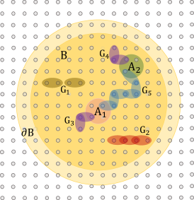
Figure 3: To study the correlations between regions $A_{1},A_{2}$, we can restrict the Gibbs state to region $B$ while adding an operator on the boundary $\partial B$ to include the effect of the rest of the lattice. Regions $G_{1},\dots,G_{5}$ show up when studying the derivatives of the correlation function. See the proofs of Theorem 31 and Theorem 32.

The proof follows from Lemma 28. We first consider a perturbed version of (58) using Definition 30. We define $f(z_{1},\dots,z_{m})$ as

$$f(z_{1},\dots,z_{m}) =\log\left(\frac{\operatorname{tr}[\rho_{\vec{z}}(H|N_{2})N_{1}]}{\operatorname{tr}[\rho_{\vec{z}}(H|\mathds{1})N_{1}]}\right)$$

$$=\log\left(\frac{\operatorname{tr}[e^{-\sum_{i=1}^{m}z_{i}H_{i}}N_{2}N_{1}]}{\operatorname{tr}[e^{-\sum_{i=1}^{m}z_{i}H_{i}}N_{2}]}\frac{\operatorname{tr}[e^{-\sum_{i=1}^{m}z_{i}H_{i}}]}{\operatorname{tr}[e^{-\sum_{i=1}^{m}z_{i}H_{i}}N_{1}]}\right).$$ (59)

This function is our choice for $f(z_{1},\dots,z_{m})$ in Lemma 28. In particular, we prove that assuming Condition 1 is satisfied, $f(z_{1},\dots,z_{m})$ is analytic in $\Omega_{\delta,\beta_{c}}$, has a bounded absolute value, and has vanishing derivatives at $z_{1}=\dots=z_{m}=0$. Let us begin with the analyticity and boundedness.

Analyticity and boundedness:

From (52) we see that for any positive operator $N$, the post-selected free energy is analytic and there exists some constant $c$ such that

$$\left|\log\left(\operatorname{tr}\left[e^{-\sum_{i=1}^{m}z_{i}H_{i}}N\right]\right)\right|\leq cn,$$ (60)

By using a proper choice for $N$, we see that $f(z_{1},\dots,z_{m})$ is a sum of analytic functions and therefore is itself analytic. We also get an upper bound on $|f(z_{1},\dots,z_{m})|$, that is,

$$\forall(z_{1},\dots,z_{m})\in\Omega_{\delta,\beta_{c}},\quad\left|f(z_{1},\dots,z_{m})\right| \leq\left|\log\left(\operatorname{tr}[e^{-\sum_{i=1}^{m}z_{i}H_{i}}N_{2}N_{1}]\right)\right|+\left|\log\left(\operatorname{tr}[e^{-\sum_{i=1}^{m}z_{i}H_{i}}N_{2}]\right)\right|$$

$$+\left|\log\left(\operatorname{tr}[e^{-\sum_{i=1}^{m}z_{i}H_{i}}N_{1}]\right)\right|+\left|\log\left(\operatorname{tr}[e^{-\sum_{i=1}^{m}z_{i}H_{i}}]\right)\right|$$

$$\leq 4cn.$$ (61)

Vanishing derivatives:

It remains to show that certain derivatives of $f(z_{1},\dots,z_{m})$ are zero at the point $\beta=0$, which is inside $\Omega_{\delta,\beta_{c}}$. The derivatives of $f(z_{1},\dots z_{m})$ are combinations of terms like

$$\frac{d^{K}}{d^{k_{1}}z_{i}\dots d^{k_{m}}z_{m}}\log\left(\operatorname{tr}\left[e^{-\sum_{i=1}^{m}z_{i}H_{i}}N_{2}N_{1}\right]\right)\Bigr{|}_{z=0},$$ (62)

where $k_{i}\geq 0$ and $K=\sum_{i=1}^{m}k_{i}$. Notice that we are including the $z_{i}$ that are not in the derivative by letting $k_{i}=0$. We claim in certain instances that these terms are either zero or cancel each other. Consider all the local terms $H_{i}$ that we are taking a derivative with respect to their $z_{i}$, i.e. $k_{i}\geq 1$. We denote the union of the support of these terms by $G$. Recall that $A_{1},A_{2}$ are the support of $O_{1},O_{2}$, respectively. Region $G$ fits into one of the following cases.

Case 1: $G$ is not connected and does not intersect with $A_{1}\cup A_{2}$ (see $G_{1}$ in Figure 3 for an example). In this case, the terms in the derivatives are

$$\frac{d^{K}}{d^{k_{1}}z_{i}\dots d^{k_{m}}z_{m}}\log\left(\operatorname{tr}\left[e^{-\sum_{i=1}^{m}z_{i}H_{i}}N_{2}N_{1}\right]\right)\Bigr{|}_{z=0} =\frac{d^{K}}{d^{k_{1}}z_{i}\dots d^{k_{m}}z_{m}}\log\left(\operatorname{tr}[N_{2}]\operatorname{tr}[N_{1}]\prod_{i\mathrel{\mathop{\mathchar 58\relax}}k_{i}\geq 1}\operatorname{tr}\left[e^{-z_{i}H_{i}}\right]\right)\Bigr{|}_{z=0}$$

$$=\frac{d^{K}}{d^{k_{1}}z_{i}\dots d^{k_{m}}z_{m}}\log\left(\operatorname{tr}[N_{2}]\operatorname{tr}[N_{1}]\right)$$

$$+\sum_{i\mathrel{\mathop{\mathchar 58\relax}}k_{i}\geq 1}\frac{d^{K}}{d^{k_{1}}z_{i}\dots d^{k_{m}}z_{m}}\log\left(\operatorname{tr}\left[e^{-z_{i}H_{i}}\right]\right)\Bigr{|}_{z=0}$$

$$=0.$$ (63)

In the first line, we used the fact that sublattices $A_{1}$, $A_{2}$, and $\operatorname{supp}(H_{i})$ with $k_{i}\geq 1$ do not intersect. The last line follows because $\operatorname{tr}[N_{2}]\operatorname{tr}[N_{1}]$ is a constant, and $\operatorname{tr}\left[e^{-z_{i}H_{i}}\right]$ only depends on $z_{i}$ and its derivative with respect to other $z_{i}$ is zero.

Case 2: $G$ is connected but does not intersect with $A_{1}\cup A_{2}$ (see $G_{2}$ in Figure 3 for an example). Similar to (5), we can still separate $\operatorname{tr}[N_{2}]\operatorname{tr}[N_{1}]$ from the remaining terms and their derivative is zero. Hence, we obtain

$$\frac{d^{K}}{d^{k_{1}}z_{i}\dots d^{k_{m}}z_{m}}\log\left(\operatorname{tr}\left[e^{-\sum_{i=1}^{m}z_{i}H_{i}}N_{2}N_{1}\right]\right)\Bigr{|}_{z=0}=\frac{d^{K}}{d^{k_{1}}z_{i}\dots d^{k_{m}}z_{m}}\log\left(\operatorname{tr}\left[e^{-\sum_{i\mathrel{\mathop{\mathchar 58\relax}}k_{i}\geq 1}z_{i}H_{i}}\right]\right)\Bigr{|}_{z=0}.$$ (64)

Although this term does not necessarily equal zero, the derivatives of $f(z_{1},\dots,z_{m})$ are combinations of terms like Eq. (64). These terms are all equal as we can separate traces involving $N_{2}$ and $N_{1}$ using the same argument as above, but they appear with opposite signs and thus cancel each other. More precisely, we have

$$\frac{d^{K}}{d^{k_{1}}z_{i}\dots d^{k_{m}}z_{m}}f(z_{1},\dots,z_{m})\Bigr{|}_{z=0}$$

$$=\frac{d^{K}}{d^{k_{1}}z_{i}\dots d^{k_{m}}z_{m}}\Big{(}\log\left(\operatorname{tr}[N_{2}N_{1}]\operatorname{tr}\left[e^{-\sum_{i\mathrel{\mathop{\mathchar 58\relax}}k_{i}\geq 1}z_{i}H_{i}}\right]\right)-\log\left(\operatorname{tr}[N_{2}]\operatorname{tr}\left[e^{-\sum_{i\mathrel{\mathop{\mathchar 58\relax}}k_{i}\geq 1}z_{i}H_{i}}\right]\right)$$

$$-\log\left(\operatorname{tr}[N_{1}]\operatorname{tr}\left[e^{-\sum_{i\mathrel{\mathop{\mathchar 58\relax}}k_{i}\geq 1}z_{i}H_{i}}\right]\right)+\log\left(\operatorname{tr}\left[e^{-\sum_{i\mathrel{\mathop{\mathchar 58\relax}}k_{i}\geq 1}z_{i}H_{i}}\right]\right)\Big{)}\Bigr{|}_{z=0}$$

$$=0.$$ (65)

Case 3: $G$ is connected and intersects with only one of $A_{1}$ or $A_{2}$ (see $G_{3}$ or $G_{4}$ in Figure 3 for an example). Similar to Case 2, the derivatives of $f(z_{1},\dots,z_{m})$ consist of equal terms with opposite signs and therefore vanish. Here, we show the case where $G$ only intersects $A_{2}$. The other ones similarly follow.

$$\frac{d^{K}}{d^{k_{1}}z_{i}\dots d^{k_{m}}z_{m}}f(z_{1},\dots,z_{m})\Bigr{|}_{z=0}$$

$$=\frac{d^{K}}{d^{k_{1}}z_{i}\dots d^{k_{m}}z_{m}}\Big{(}\log\left(\operatorname{tr}[N_{1}]\operatorname{tr}\left[e^{-\sum_{i\mathrel{\mathop{\mathchar 58\relax}}k_{i}\geq 1}z_{i}H_{i}}N_{2}\right]\right)-\log\left(\operatorname{tr}\left[e^{-\sum_{i\mathrel{\mathop{\mathchar 58\relax}}k_{i}\geq 1}z_{i}H_{i}}N_{2}\right]\right)$$

$$-\log\left(\operatorname{tr}[N_{1}]\operatorname{tr}\left[e^{-\sum_{i\mathrel{\mathop{\mathchar 58\relax}}k_{i}\geq 1}z_{i}H_{i}}\right]\right)+\log\left(\operatorname{tr}\left[e^{-\sum_{i\mathrel{\mathop{\mathchar 58\relax}}k_{i}\geq 1}z_{i}H_{i}}\right]\right)\Big{)}\Bigr{|}_{z=0}$$

$$=0,$$ (66)

in which the first two and last two terms cancel each other.

Case 4: $G$ is connected and intersects with both $A_{1}$ and $A_{2}$ (see $G_{5}$ in Figure 3 for an example). Here, the cancellation that appeared in the other cases does not happen. Thus, this is the only situation in which the derivatives are non-zero.

The important observation is that for Case 4 to happen, $G$ needs to be long enough to touch both $A_{1}$ and $A_{2}$. Hence, if the number of $z_{i}$ with $k_{i}\geq 1$ is less than roughly $\mathrm{dist}(O_{1},O_{2})$, their corresponding derivative vanishes. Having all the criteria needed for applying Lemma 28, i.e analyticity, boundedness, and zero derivatives, we can get the following bound on $|f(z_{1},\dots,z_{m})|$ for some constant $c$ and $\xi$:

$$|f(\beta,\dots,\beta)|\leq cne^{-\mathrm{dist}(O_{1},O_{2})/\xi},$$ (67)

which as explained before implies

$$\big{|}\operatorname{tr}\left[\rho_{\beta}(H)O_{1}O_{2}\right]-\operatorname{tr}\left[\rho_{\beta}(H)O_{1}\right]\operatorname{tr}\left[\rho_{\beta}(H)O_{2}\right]\big{|}\leq cne^{-\mathrm{dist}(O_{1},O_{2})/\xi}.$$ (68)

Due to the extra factor of $n$ in front of this bound, it implies the exponential decay of correlations only when $\mathrm{dist}(O_{1},O_{2})=\Omega(\log n)$.     $\sqcap$$\sqcup$

5.1 Tighter bounds for commuting Hamiltonians

Here we show how using the commutativity of $H$ enables us to remove the extra factor of $n$ in the bound (67) that we derived for general Hamiltonians. We state this in the following theorem.

Theorem 32.

Suppose $H$ is a geometrically-local Hamiltonian with mutually commuting terms that satisfies Condition 1 for $\beta\in[0,\beta_{c})$. Then the correlations between any two operators $O_{1},O_{2}$ decay exponentially for all $\beta\in[0,\beta_{c})$ as in Condition 2.

Proof of Theorem 32.

The proof of this theorem follows similar steps to that of Theorem 31. A crucial difference, which is the only part where we use the commutativity of local terms $H_{i}$, is the following. The Hamiltonian $H$ in states $\rho_{\beta}(H|N_{2})$ and $\rho_{\beta}(H|\mathds{1})$ involves terms acting on all $n$ sites in lattice $\Lambda$. In our analysis, we can essentially neglect the contribution of sites that are far from both region $A_{1}$ and $A_{2}$. In other words, as shown in Figure 3, let $B\subset\Lambda$ be a ball of diameter slightly larger than $\mathrm{dist}(O_{1},O_{2})$ centered at $A_{1}$ that encloses region $A_{2}$. We restrict the Hamiltonian and states $\rho_{\beta}(H|N_{2}),\rho_{\beta}(H|\mathds{1})$ to this region and include the effect of other sites by an operator acting on $\partial B$, the boundary of this enclosing region. We prove (58) for this smaller region. Without this step, we end up getting an upper bound like $cn\exp(-\mathrm{dist}(O_{1},O_{2})/\xi)$, which has an extra factor of $n$, the number of sites in $\Lambda$, whereas with the restriction to the enclosing region, this factor is the number of sites in $B$ which is negligible compared to the exponential decay factor. More formally, since $H$ is a commuting Hamiltonian, we have $e^{-\beta H}=e^{-\beta H_{B}}e^{-\beta(H-H_{B})}$. Hence, we get

$$\operatorname{tr}[\rho_{\beta}(H|N_{2})N_{1}] =\frac{\operatorname{tr}[e^{-\beta H}N_{2}N_{1}]}{\operatorname{tr}[e^{-\beta H}N_{2}]}$$

$$=\frac{\operatorname{tr}_{B}[e^{-\beta H_{B}}\operatorname{tr}_{\bar{B}}[e^{-\beta(H-H_{B})}]N_{2}N_{1}]}{\operatorname{tr}_{B}[e^{-\beta H_{B}}\operatorname{tr}_{\bar{B}}[e^{-\beta(H-H_{B})}]N_{2}]}$$

$$=\frac{\operatorname{tr}_{B}[e^{-\beta H_{B}}\sigma N_{2}N_{1}]}{\operatorname{tr}_{B}[e^{-\beta H_{B}}\sigma N_{2}]}$$

$$=\operatorname{tr}[\rho_{\beta}(H_{B}|\sigma N_{2})N_{1}],$$ (69)

where

$$\sigma=\frac{\operatorname{tr}_{\bar{B}}[e^{-\beta(H-H_{B})}]}{\operatorname{tr}_{\bar{B}\cup\partial\bar{B}}[e^{-\beta(H-H_{B})}]}$$ (70)

is a state acting on the boundary $\partial\bar{B}$ . Thus, we can replace the operator $N_{2}$ by $\sigma\otimes N_{2}$ acting on a larger region $\partial\bar{B}\cup A_{2}$, which is still only a constant, and restrict our attention to region $B$. We can now repeat the argument of Theorem 31. Let the perturbed Hamiltonian restricted to region $B$ be $H_{B}(\vec{z})=\sum_{H_{i}\mathrel{\mathop{\mathchar 58\relax}}\operatorname{supp}(H_{i})\subset B}z_{i}H_{i}$, where for simplicity, the number of local terms in $H_{B}$ is denoted again by $m$. By plugging (69) into (5), we see that the function $f(z_{1},\dots,z_{m})$ is

$$f(z_{1},\dots,z_{m}) =\log\left(\frac{\operatorname{tr}[\rho_{\vec{z}}(H_{B}|\sigma N_{2})N_{1}]}{\operatorname{tr}[\rho_{\vec{z}}(H_{B}|\sigma)N_{1}]}\right)$$

$$=\log\left(\frac{\operatorname{tr}[e^{-\beta H_{B}(\vec{z})}\sigma N_{2}N_{1}]}{\operatorname{tr}[e^{-H_{B}(\vec{z})}\sigma N_{2}]}\frac{\operatorname{tr}[e^{-\beta H_{B}(\vec{z})}\sigma]}{\operatorname{tr}[e^{-\beta H_{B}(\vec{z})}\sigma N_{1}]}\right)$$ (71)

The rest of the proof of Theorem 31 applies to this function. In particular, assuming Condition 1 holds, this function is bounded and analytic in $\Omega_{\delta,\beta_{c}}$, i.e. $|f(z_{1},\dots,z_{m})|\leq c|B|$. Similarly, one can see that the low-order derivatives of $f(z_{1},\dots,z_{m})$ are zero. Since the distance between $\partial{B}$ and $A_{1}$ is still $O(\mathrm{dist}(O_{1},O_{2}))$, Lemma 28 implies $|f(\beta,\dots,\beta)|\leq c|B|\exp(-\mathrm{dist}(O_{1},O_{2})/\xi)$. Hence, we have

$$\big{|}\operatorname{tr}\left[\rho_{\beta}(H)O_{1}O_{2}\right]-\operatorname{tr}\left[\rho_{\beta}(H)O_{1}\right]\operatorname{tr}\left[\rho_{\beta}(H)O_{2}\right]\big{|}\leq c\ \mathrm{dist}(O_{1},O_{2})^{D}e^{-\mathrm{dist}(O_{1},O_{2})/\xi}.$$ (72)

$\sqcap$$\sqcup$

5.2 Tighter bounds for 1D Hamiltonians

Theorem 33.

Let $H$ be a geometrically-local Hamiltonian on a $1D$ chain that satisfies Condition 1. Then, the exponential decay of correlations given in Condition 2 also holds for this Hamiltonian.

Proof of Theorem 33.

The proof is similar to that of Theorem 31 and Theorem 32. Recall that an important step is to introduce boundary states $\sigma$ that include the effect of terms in the Hamiltonian $H$ that are acting on the boundary or outside of some region $B$. Region $B$ encloses the support of operators whose correlations we want to bound. There, we use the commutativity of $H$ to find the boundary states $\sigma$ which does not hold in general. Here, we show how, by using the quantum belief propagation operator $\eta$ we introduced in Proposition 14, we can achieve the same boundary state in $1$D.

We do not go through all steps of the proof of Theorem 31 again. Instead, we directly show that by restricting the Hamiltonian to region $B$ and adding the boundary terms, the covariance in (53) changes negligibly. Then we apply bound (68) to this restricted covariance. Since the number of particles inside $B$ is constant, instead of the extra factor of $n$, we get a constant prefactor as desired.

Recall that using the belief propagation equation (14) and the bound (15), we can remove the boundary terms $H_{\partial B}$ acting between $B,\bar{B}$ from the Gibbs state and get

$$\operatorname{tr}[\rho_{\beta}(H)O_{1}O_{2}] =\operatorname{tr}\left[\frac{Z_{\beta}(H-H_{\partial B})}{Z_{\beta}(H)}\eta\rho_{\beta}(H-H_{\partial B})\eta^{{\dagger}}O_{1}O_{2}\right]$$

$$=\operatorname{tr}\left[\frac{Z_{\beta}(H-H_{\partial B})}{Z_{\beta}(H)}\eta_{\ell}\rho_{\beta}(H-H_{\partial B})\eta^{{\dagger}}_{\ell}O_{1}O_{2}\right]$$

$$+\operatorname{tr}\left[\frac{Z_{\beta}(H-H_{\partial B})}{Z_{\beta}(H)}\eta_{\ell}\rho_{\beta}(H-H_{\partial B})(\eta^{{\dagger}}-\eta_{\ell}^{{\dagger}})O_{1}O_{2}\right]$$

$$+\operatorname{tr}\left[\frac{Z_{\beta}(H-H_{\partial B})}{Z_{\beta}(H)}(\eta-\eta_{\ell})\rho_{\beta}(H-H_{\partial B})\eta^{{\dagger}}O_{1}O_{2}\right],$$ (73)

where in the second line, we replaced $\eta$ with the truncated operator $\eta_{\ell}$. To simplify this equation, we absorb the coefficient $Z_{\beta}(H-H_{\partial B})/Z_{\beta}(H)$ into the operators $\eta,\eta_{\ell}$, and define

$$\tilde{\eta}=\left(\frac{Z_{\beta}(H-H_{\partial B})}{Z_{\beta}(H)}\right)^{1/2}\eta,\quad\tilde{\eta}_{\ell}=\left(\frac{Z_{\beta}(H-H_{\partial B})}{Z_{\beta}(H)}\right)^{1/2}\eta_{\ell}.$$ (74)

Hence, we have

$$\left|\operatorname{tr}\left[\rho_{\beta}(H)O_{1}O_{2}\right]-\operatorname{tr}\left[\tilde{\eta}_{\ell}\rho_{\beta}(H-H_{\partial B})\tilde{\eta}^{{\dagger}}_{\ell}O_{1}O_{2}\right]\right| \leq\left|\operatorname{tr}\left[\tilde{\eta}\rho_{\beta}(H-H_{\partial B})(\tilde{\eta}^{{\dagger}}-\tilde{\eta}_{\ell}^{{\dagger}})O_{1}O_{2}\right]\right|$$

$$+\left|\operatorname{tr}\left[(\tilde{\eta}-\tilde{\eta}_{\ell})\rho_{\beta}(H-H_{\partial B})\tilde{\eta}^{{\dagger}}O_{1}O_{2}\right]\right|.$$ (75)

According to (15), we have ${||\eta-\eta_{\ell}||}\leq e^{\alpha_{1}|\partial B|-\alpha_{2}\ell}$ and ${||\eta||}\leq e^{\beta/2{||H_{\partial B}||}}$. Also, Lemma 22 implies $Z_{\beta}(H-H_{\partial B})/Z_{\beta}(H)\leq e^{\alpha_{3}|\partial B|}$ for some constant $\alpha_{3}$ that depends on the details of $H$. Using these bounds as well as the Cauchy-Schwarz and Hölder inequalities, we get the following bound for some constants $c^{\prime}$ and $\alpha_{4}$:

$$\left|\operatorname{tr}\left[\rho_{\beta}(H)O_{1}O_{2}\right]-\operatorname{tr}\left[\tilde{\eta}_{\ell}\rho_{\beta}(H-H_{\partial B})\tilde{\eta}^{{\dagger}}_{\ell}O_{1}O_{2}\right]\right| \leq 2{||O_{1}||}{||O_{2}||}{||\eta-\eta_{\ell}||}{||\eta||}$$

$$\leq c^{\prime}e^{-\alpha_{4}\ell}.$$ (76)

To arrive at the last line, we used the fact that $|\partial B|$ in $1$D is just a constant that depends on the range of $H$, and we assumed the truncation length $\ell$ is sufficiently larger than $|\partial B|$.

Note that since we removed the boundary terms $H_{\partial B}$, the Gibbs state decomposes into $\rho_{\beta}(H-H_{\partial B})=\rho_{\beta}(H_{\bar{B}})\rho_{\beta}(H_{B})$, which allows us to write

$$\operatorname{tr}\left[\tilde{\eta}_{\ell}\rho_{\beta}(H-H_{\partial B})\tilde{\eta}^{{\dagger}}_{\ell}O_{1}O_{2}\right]=\operatorname{tr}\left[\rho_{\beta}(H_{B})\tilde{\sigma}_{\partial B}O_{1}O_{2}\right],$$ (77)

in which we assume region $B$ is chosen to be wide enough so that both $O_{1},O_{2}$ are sufficiently far from the boundary $\partial B$ compared to length $\ell$. This means $\eta_{\ell}$ does not overlap with $O_{1},O_{2}$. We also define the unnormalized boundary state $\tilde{\sigma}_{\partial B}$ by

$$\tilde{\sigma}_{\partial B}=\tilde{\eta}^{{\dagger}}_{\ell}\tilde{\eta}_{\ell}\operatorname{tr}_{\bar{B}\setminus{\operatorname{supp}(\eta_{\ell})}}[\rho_{\beta}(H_{\bar{B}})].$$ (78)

Notice that $\tilde{\sigma}_{\partial B}$ is a PSD matrix. To see why, we use the fact that $\operatorname{tr}_{\bar{B}\setminus{\operatorname{supp}(\eta_{\ell})}}[\rho_{\beta}(H_{\bar{B}})]$ is a PSD matrix and hence can be written as $WW^{{\dagger}}$ for some operator $W$ supported on $\operatorname{supp}(\eta_{\ell})\cap\bar{B}$. Then it is not hard to see that for any state $|\phi\rangle$, we have

$$\langle\phi|\tilde{\sigma}_{\partial B}|\phi\rangle=\sum_{i=1}^{\dim(\operatorname{supp}(W))}\langle i|W^{{\dagger}}\langle\phi|\tilde{\eta}_{\ell}^{{\dagger}}\tilde{\eta}_{\ell}W|i\rangle|\phi\rangle\geq 0.$$ (79)

Overall, we have

$$\left|\operatorname{tr}\left[\rho_{\beta}(H)O_{1}O_{2}\right]-\operatorname{tr}\left[\rho_{\beta}(H_{B})\tilde{\sigma}_{\partial B}O_{1}O_{2}\right]\right|\leq c^{\prime}e^{-\alpha_{4}\ell}.$$ (80)

Similarly, we can replace $\operatorname{tr}[\rho_{\beta}(H)O_{i}]$ with $\operatorname{tr}[\rho_{\beta}(H_{B})\tilde{\sigma}_{\partial B}O_{i}]$ up to an exponentially small error in $\ell$,

$$\left|\operatorname{tr}\left[\rho_{\beta}(H)O_{i}\right]-\operatorname{tr}\left[\rho_{\beta}(H_{B})\tilde{\sigma}_{\partial B}O_{i}\right]\right|\leq c^{\prime}e^{-\alpha_{4}\ell},\quad i\in\{1,2\}.$$ (81)

We can now plug these expressions into the covariance (53). Since ${||\operatorname{tr}[\rho_{\beta}(H_{B})\tilde{\sigma}_{\partial B}O_{i}]||}$ is just a constant, we see that there exist constants $c^{\prime\prime}$ and $\alpha_{5}$ such that

$$\big{|}\operatorname{tr}\left[\rho_{\beta}(H)O_{1}O_{2}\right]-\operatorname{tr}\left[\rho_{\beta}(H)O_{1}\right]\operatorname{tr}\left[\rho_{\beta}(H)O_{2}\right]\big{|}$$

$$=\big{|}\left(\operatorname{tr}\left[\rho_{\beta}(H_{B})\tilde{\sigma}_{\partial B}O_{1}O_{2}\right]+c^{\prime}e^{-\alpha_{4}\ell}\right)-\left(\operatorname{tr}\left[\rho_{\beta}(H_{B})\tilde{\sigma}_{\partial B}O_{1}\right]-c^{\prime}e^{-\alpha_{4}\ell}\right)\left(\operatorname{tr}\left[\rho_{\beta}(H)\tilde{\sigma}_{\partial B}O_{2}\right]-c^{\prime}e^{-\alpha_{4}\ell}\right)\big{|}$$

$$\leq\big{|}\operatorname{tr}\left[\rho_{\beta}(H_{B})\tilde{\sigma}_{\partial B}O_{1}O_{2}\right]-\operatorname{tr}\left[\rho_{\beta}(H_{B})\tilde{\sigma}_{\partial B}O_{1}\right]\operatorname{tr}\left[\rho_{\beta}(H)\tilde{\sigma}_{\partial B}O_{2}\right]\big{|}+c^{\prime\prime}e^{-\alpha_{5}\ell}.$$ (82)

We can consider $\tilde{\sigma}_{\partial B}O_{2}$ to be the new operator whose correlation with $O_{1}$ we want to measure. The operator $\tilde{\sigma}_{\partial B}O_{2}$ is still $\mathrm{dist}(O_{1},O_{2})$ far from $O_{1}$. Thus, using the bound (68) proved in Theorem 31, we get

$$\big{|}\operatorname{tr}\left[\rho_{\beta}(H_{B})\tilde{\sigma}_{\partial B}O_{1}O_{2}\right]-\operatorname{tr}\left[\rho_{\beta}(H_{B})\tilde{\sigma}_{\partial B}O_{1}\right]\operatorname{tr}\left[\rho_{\beta}(H)\tilde{\sigma}_{\partial B}O_{2}\right]\big{|}\leq c|B|e^{-\mathrm{dist}(O_{1},O_{2})/\xi}.$$ (83)

Combined with (82), we have

$$\big{|}\operatorname{tr}\left[\rho_{\beta}(H)O_{1}O_{2}\right]-\operatorname{tr}\left[\rho_{\beta}(H)O_{1}\right]\operatorname{tr}\left[\rho_{\beta}(H)O_{2}\right]\big{|}\leq c|B|e^{-\mathrm{dist}(O_{1},O_{2})/\xi}+c^{\prime\prime}e^{-\alpha_{5}\ell}.$$ (84)

Since all the coefficients in the bound on the right-hand side are constants, it suffices to choose $\ell$ large enough compared to $\mathrm{dist}(O_{1},O_{2})$ so that it is negligible compared to the $e^{-\mathrm{dist}(O_{1},O_{2})/\xi}$ term. This is possible because we assumed $\partial{C}$ is sufficiently (but still only constantly) far from $O_{1},O_{2}$. This allows us to get a bound that does not depend on $n$ as before, hence finishing the proof.     $\sqcap$$\sqcup$

Remark 34.

Recall that from (15) we know that the error of truncating the belief propagation operator $\eta$ is

$${\big{|}\big{|}\eta-\eta_{\ell}\big{|}\big{|}}\leq e^{\alpha_{1}|\partial B|-\alpha_{2}\ell}.$$ (85)

In our setting, the dependence of the error bound on $e^{\alpha_{1}|\partial B|}$ makes this result only be applicable when $\Lambda$ is a $1$D lattice. Otherwise, since $|\partial B|$ is proportional to $\operatorname{diam}(B)^{D-1}$, we cannot choose length $\ell$ small enough compared to $\operatorname{diam}(B)$. Hence, we do not get a local operator as required.

6 Exponential decay of correlations implies analyticity

In this section, we focus on the converse of Theorem 31. In Section 5, we showed that the exponential decay of correlations is a necessary condition for the analyticity of the free energy. In this section, we ask if this condition is also sufficient for the analyticity. This was first established for classical systems by Dobrushin and Shlosman [DS87]. It appears that the quantum generalization of that proof requires the development of new tools. The goal in this section is to identify these tools. Our contribution is to extend the result of [DS87] to classical systems that are not translationally invariant and express the proof in a language that is suitable for the quantum case.

Here, for clarity, we consider a simpler version of Condition 1 that is stated below:

Condition 1’ (Analyticity of the free energy).

The free energy of a geometrically-local Hamiltonian $H$ is $\delta$-analytic at inverse temperature $\beta\in\mathbb{R}^{+}$ if for all $\beta^{\prime}\in\mathbb{C}$ such that $|\beta^{\prime}-\beta|\leq\delta$, the free energy is analytic and there exists a constants $c$ such that

$$\left|\log\left(\operatorname{tr}\left[e^{-\beta^{\prime}H}\right]\right)\right|\leq cn.$$ (86)

Recall that in Condition 1, we assumed that the free energy of a post-selected state is analytic and bounded. In comparison, Condition 1’ only includes partition functions with an open boundary condition. For algorithmic purposes, like the one in Section 3, this version is sufficient. However, with small modifications, the same proof can be adapted to show Condition 1 with arbitrary boundary conditions.

Our goal is to derive Condition 1’ assuming that the correlations in the system decay exponentially. We restate this condition for convenience.

Restatement of Condition 2. The correlations in the Gibbs state $\rho_{\beta}(H)$ of a geometrically-local Hamiltonian decay exponentially if for any local Hermitian operators $O_{1}$ and $O_{2}$, there exist constants $\xi$ and $c$ such that

$$\big{|}\operatorname{tr}\left[\rho_{\beta}(H)O_{1}O_{2}\right]-\operatorname{tr}\left[\rho_{\beta}(H)O_{1}\right]\operatorname{tr}\left[\rho_{\beta}(H)O_{2}\right]\big{|}\leq c{||O_{1}||}{||O_{2}||}e^{-\mathrm{dist}(O_{1},O_{2})/\xi}.$$ (87)

Although we consider classical systems, we find it more convenient to continue using quantum notation. This also makes it easier to point out where the proof breaks for quantum systems. The reader, however, should note that the terms in the Hamiltonian are all diagonal in a product basis and the projector operators we use basically fix the value of classical spins.

More formally, we prove the following theorem in this section.

Theorem 35 (The decay of correlations implies analyticity for classical systems).

Let $H=\sum_{i=1}^{m}H_{i}$ be a geometrically-local Hamiltonian of a classical spin system, i.e. the local terms $H_{i}$ are all diagonal in the same product basis. For such a system, the exponential decay of correlations given in Condition 2 implies analyticity of the free energy in Condition 1’.

Figure 4: The structure of the proof of Theorem 35. We follow a series of reductions to show Condition 1’.

We prove this theorem in multiple steps that are formulated in Propositions 36, 37, and 39. An outline of the proof is given in Figure 4. It turns out that Proposition 36 and Proposition 37 continue to hold for commuting Hamiltonians, so we give their statements and proofs for these Hamiltonians. However, for reasons to be highlighted in its proof, Proposition 39 only holds for classical systems.

Proof of Theorem 35.

The proof is immediate from the combination of Proposition 37, Proposition 36, and Proposition 39.     $\sqcap$$\sqcup$

6.1 Step 1: Condition 1’ from the complex site removal bound

Our first step, stated in Proposition 36, is to show how a variant of the complex site removal bound that we discussed in Section 4 allows us to find an upper bound on the absolute value of the free energy as in Condition 1’. Compared to the bound (25) in Section 4, this variant includes setting a non-trivial boundary condition after removing a subset of lattice sites. To avoid subtleties arising from entangled boundary conditions and projectors, we need to give a slightly different proof compared to what we did before (24).

Proposition 36 (Condition 1’ from the complex site removal bound).

Let $H=\sum_{k=1}^{m}H_{k}$ be a geometrically-local Hamiltonian with mutually commuting terms on lattice $\Lambda$. Let $P$ be a projector acting on $\partial\bar{A}$ where $A\subset\Lambda$ is a region of constant size. We denote the terms in $H$ acting on $\bar{A}$ or $\partial\bar{A}$ by $H^{\prime}$ and the real and imaginary parts of $\beta\in\mathbb{C}$ by $\beta_{r}$ and $\beta_{i}$. Suppose when $|\beta_{i}|\leq\delta$ for some sufficiently small $\delta$, there exists a constant $c$ such that

$$\left|\log\left(\frac{\operatorname{tr}_{\bar{A}\cup A}[e^{-\beta H}]}{\operatorname{tr}_{\bar{A}\cup\partial\bar{A}}\left[e^{-\beta H^{\prime}}P\right]}\right)\right|\leq c.$$ (88)

Then,

• The observables supported on $A$ like $H_{A}$ have bounded expectations with respect to the complex perturbed Gibbs state $\rho_{\beta}(H)$. That is, there exists a constant $c^{\prime}$ such that $|\operatorname{tr}\left[H_{A}\rho_{\beta}(H)\right]|\leq c^{\prime}{||H_{A}||}.$

• Condition 1’ holds for this system.

Proof of Proposition 36.

By using Lemma 22, we have $|\log(\operatorname{tr}[e^{-\beta_{r}H}])|\leq O(n)$. Hence to show (86), it is sufficient to show that

$$\left|\log\left(\frac{\operatorname{tr}[e^{-\beta H}]}{\operatorname{tr}[e^{-\beta_{r}H}]}\right)\right|\leq cn.$$ (89)

The difference between the numerator and denominator of (89) is the addition of the complex perturbations $\beta_{i}H=\sum_{k=1}^{m}\beta_{i}H_{k}$ to the exponent of the numerator. Instead of adding these terms all together, we can add local terms $\beta_{i}H_{k}$ step by step. We do this by setting up a telescoping series of products such that in each fraction, a new term $\beta_{i}H_{k}$ is added. We have

$$\frac{\operatorname{tr}[e^{-\beta H}]}{\operatorname{tr}[e^{-\beta_{r}H}]}=\frac{\operatorname{tr}[e^{-\beta_{r}H-i\beta_{i}\sum_{k=1}^{m}H_{k}}]}{\operatorname{tr}[e^{-\beta_{r}H-i\beta_{i}\sum_{k=1}^{m-1}H_{k}}]}\frac{\operatorname{tr}[e^{-\beta_{r}H-i\beta_{i}\sum_{k=1}^{m-1}H_{k}}]}{\operatorname{tr}[e^{-\beta_{r}H-i\beta_{i}\sum_{k=1}^{m-2}H_{k}}]}\dots\frac{\operatorname{tr}[e^{-\beta_{r}H-i\beta_{i}H_{1}}]}{\operatorname{tr}[e^{-\beta_{r}H}]}.$$ (90)

Hence,

$$\left|\log\left(\frac{\operatorname{tr}[e^{-\beta H}]}{\operatorname{tr}[e^{-\beta_{r}H}]}\right)\right|\leq\sum_{j=0}^{m-1}\left|\log\left(\frac{\operatorname{tr}[e^{-\beta_{r}H-i\beta_{i}\sum_{k=0}^{j+1}H_{k}}]}{\operatorname{tr}[e^{-\beta_{r}H-i\beta_{i}\sum_{k=0}^{j}H_{k}}]}\right)\right|,$$ (91)

in which we set $H_{0}=0$. Since for interactions considered in this paper $m=O(n)$, we can derive the bound in (99) by showing for any $j$,

$$\left|\log\left(\frac{\operatorname{tr}[e^{-\beta_{r}H-i\beta_{i}\sum_{k=0}^{j+1}H_{k}}]}{\operatorname{tr}[e^{-\beta_{r}H-i\beta_{i}\sum_{k=0}^{j}H_{k}}]}\right)\right|\leq O(1).$$ (92)

To do so, we define $\gamma_{j}(t)$ for $t\in[0,1]$ to be

$$\gamma_{j}(t)=\log\left(\operatorname{tr}[e^{-\beta_{r}H-i\beta_{i}\sum_{k=0}^{j}H_{k}-i\beta_{i}tH_{j+1})}]\right).$$ (93)

Then, the left hand side of (92) can be written as

$$\left|\log\left(\frac{\operatorname{tr}[e^{-\beta_{r}H-i\beta_{i}\sum_{k=0}^{j+1}H_{k}}]}{\operatorname{tr}[e^{-\beta_{r}H-i\beta_{i}\sum_{k=0}^{j}H_{k}}]}\right)\right| =|\gamma_{j}(1)-\gamma_{j}(0)|$$

$$\leq\max_{t\in[0,1]}\left|\frac{d\gamma_{j}(t)}{dt}\right|$$

$$=|\beta_{i}|\max_{t\in[0,1]}\left|\frac{\operatorname{tr}[H_{j+1}e^{-it\beta_{i}H_{j+1}}e^{-\beta_{r}H-i\beta_{i}\sum_{k=0}^{j}H_{k}}]}{\operatorname{tr}[e^{-it\beta_{i}H_{j+1}}e^{-\beta_{r}H-i\beta_{i}\sum_{k=0}^{j}H_{k}}]}\right|.$$ (94)

For a region $A\subset\Lambda$, let $H_{A}$ and $H^{\prime}$ be parts of the Hamiltonian acting on $A$ and $\bar{A}\cup\partial\bar{A}$, respectively. One can see that for any choice of $j$ and $t$, finding an upper bound like the one in (94) is equivalent to bounding a local expectation term like

$$\operatorname{tr}\left[H_{A}e^{-(\beta_{r}+it\beta_{i})H_{A}}\frac{e^{-\beta H^{\prime}}}{Z_{\beta}(H)}\right]=\operatorname{tr}[H_{A}\rho_{\beta}(H)]$$ (95)

for some suitable choice of $A$. We also assume, without loss of generality, that all local terms in $H^{\prime}$ are complex perturbed. Using the Hölder inequality, we get

$$\left|\operatorname{tr}\left[H_{A}e^{-(\beta_{r}+it\beta_{i})H_{A}}\frac{e^{-\beta H^{\prime}}}{Z_{\beta}(H)}\right]\right| =\left|\operatorname{tr}_{A}\left[H_{A}e^{-(\beta_{r}+it\beta_{i})H_{A}}\frac{\operatorname{tr}_{\bar{A}}[e^{-\beta H^{\prime}}]}{Z_{\beta}(H)}\right]\right|$$

$$\leq{||H_{A}||}e^{|\beta|{||H_{A}||}}d^{|\partial\bar{A}|}{\Big{|}\Big{|}\frac{\operatorname{tr}_{\bar{A}}[e^{-\beta H^{\prime}}]}{Z_{\beta}(H)}\Big{|}\Big{|}}.$$ (96)

Since $|A|=O(1)$, we only need to upper bound the largest singular value of $\operatorname{tr}_{\bar{A}}[e^{-\beta H^{\prime}}]/Z_{\beta}(H)$, whose support is only on $\partial\bar{A}$, by a constant. Let $|u\rangle$ and $|v\rangle$ be the left and right singular vectors associated with the largest singular value. We claim that there exists a rank $1$ projector $P$ supported on $\partial\bar{A}$ such that

$${\Big{|}\Big{|}\frac{\operatorname{tr}_{\bar{A}}[e^{-\beta H^{\prime}}]}{Z_{\beta}(H)}\Big{|}\Big{|}} =\operatorname{tr}_{\partial\bar{A}}\left[\frac{\operatorname{tr}_{\bar{A}}[e^{-\beta H^{\prime}}]}{Z_{\beta}(H)}|u\rangle\langle v|\right]$$

$$\leq(2+\sqrt{2})\left|\operatorname{tr}_{\bar{A}\cup\partial\bar{A}}\left[\frac{e^{-\beta H^{\prime}}}{Z_{\beta}(H)}P\right]\right|.$$ (97)

This can be derived by noting that $|u\rangle\langle v|$ can be decomposed as sum of rank $1$ projectors as follows

$$|u\rangle\langle v|=-\frac{1+i}{2}\left(|u\rangle\langle u|+|v\rangle\langle v|\right)+i|w^{-}\rangle\langle w^{-}|+|w^{+}\rangle\langle w^{+}|,$$ (98)

where $|w^{+}\rangle=\frac{1}{\sqrt{2}}(|u\rangle+|v\rangle)$ and $|w^{-}\rangle=\frac{1}{\sqrt{2}}(|u\rangle+i|v\rangle)$.

Finally, using the premise of this proposition given in (88), we get both (i.) and Condition 1’, which concludes the proof.     $\sqcap$$\sqcup$

6.2 Step 2: The complex site removal bound from the small relative phase condition

Proposition 37.

Consider the same setup as that of Proposition 36. Let $P$ and $Q$ be projectors acting on $\partial\bar{A}$. Let $\theta(\delta)$ be a complex function depending on $H$, $P$, and $Q$, but constant in $n$ such that for any positive constant $c$, $c|\theta(\delta)|\geq\delta$ for sufficiently small $\delta$. We can, for instance, assume $|\theta(\delta)|=\sqrt{\delta}$. Suppose when $|\beta_{i}|\leq\delta$ for some sufficiently small $\delta$, we have

$$\frac{\operatorname{tr}_{\bar{A}\cup\partial\bar{A}}[e^{-i\beta_{i}H^{\prime}}\rho_{\beta_{r}}(H^{\prime}|P)]}{\operatorname{tr}_{\bar{A}\cup\partial\bar{A}}[e^{-i\beta_{i}H^{\prime}}\rho_{\beta_{r}}(H^{\prime}|Q)]}=1+|\partial\bar{A}|\theta(\delta).$$ (99)

Then, the complex site removal bound (88) given in Proposition 36 holds, i.e.

$$\left|\log\left(\frac{\operatorname{tr}_{\bar{A}\cup A}\left[e^{-\beta H}\right]}{\operatorname{tr}_{\bar{A}\cup\partial\bar{A}}\left[e^{-\beta H^{\prime}}P\right]}\right)\right|\leq c.$$ (100)

Before getting to the proof of this proposition, we first state and prove a relevant lemma.

Lemma 38.

Consider the same definitions as in Proposition 37. The ratio of the unperturbed partition functions (with real $\beta$) with different boundary conditions can be bounded as

$$\left|\log\left(\frac{\operatorname{tr}_{\bar{A}\cup\partial\bar{A}}\left[e^{-\beta_{r}H^{\prime}}Q\right]}{\operatorname{tr}_{\bar{A}\cup\partial\bar{A}}\left[e^{-\beta_{r}H^{\prime}}P\right]}\right)\right|\leq c^{\prime}$$ (101)

for some constant $c^{\prime}$ depending on $|\partial{\bar{A}}|$.

Proof of Lemma 38.

Let $H_{\bar{A}}$ be terms in $H^{\prime}$ that are acting solely on $\bar{A}$. That is, $H_{\bar{A}}$ commutes with both $P$ and $Q$. We have

$$\frac{\operatorname{tr}_{\bar{A}\cup\partial\bar{A}}\left[e^{-\beta_{r}H^{\prime}}Q\right]}{\operatorname{tr}_{\bar{A}\cup\partial\bar{A}}\left[e^{-\beta_{r}H^{\prime}}P\right]}=\frac{\operatorname{tr}_{\bar{A}\cup\partial\bar{A}}\left[e^{-\beta_{r}H^{\prime}}Q\right]}{\operatorname{tr}_{\bar{A}\cup\partial\bar{A}}\left[e^{-\beta_{r}H_{\bar{A}}}Q\right]}\frac{\operatorname{tr}_{\bar{A}\cup\partial\bar{A}}\left[e^{-\beta_{r}H_{\bar{A}}}P\right]}{\operatorname{tr}_{\bar{A}\cup\partial\bar{A}}\left[e^{-\beta_{r}H^{\prime}}P\right]}.$$ (102)

We can bound both of the ratios on the left side of this equality as follows:

$$\left|\frac{\operatorname{tr}_{\bar{A}\cup\partial\bar{A}}\left[e^{-\beta_{r}H^{\prime}}Q\right]}{\operatorname{tr}_{\bar{A}\cup\partial\bar{A}}\left[e^{-\beta_{r}H_{\bar{A}}}Q\right]}\right|=\left|\operatorname{tr}_{\bar{A}\cup\partial\bar{A}}\left[e^{-\beta_{r}(H^{\prime}-H_{\bar{A}})}\rho_{\beta}(H_{\bar{A}}|Q)\right]\right|\leq{\big{|}\big{|}e^{-\beta_{r}(H^{\prime}-H_{\bar{A}})}\big{|}\big{|}}.$$ (103)

Similarly, we can exchange the role of $P$ and $Q$ to get a lower bound.     $\sqcap$$\sqcup$

Proof of Proposition 37.

We show how assuming equation (99), we can derive a lower and an upper bound for

$$\left|\frac{\operatorname{tr}_{\bar{A}\cup A}\left[e^{-\beta H}\right]}{\operatorname{tr}_{\bar{A}\cup\partial\bar{A}}\left[e^{-\beta H^{\prime}}P\right]}\right|.$$ (104)

We decompose the expression (104) into two parts denoted by $L_{1}$ and $L_{2}$ as follows

$$\frac{\operatorname{tr}_{\bar{A}\cup A}\left[e^{-\beta H}\right]}{\operatorname{tr}_{\bar{A}\cup\partial\bar{A}}\left[e^{-\beta H^{\prime}}P\right]} =\operatorname{tr}_{A}\left[e^{-i\beta_{i}H_{A}}e^{-\beta_{r}H_{A}}\frac{\operatorname{tr}_{\bar{A}}\left[e^{-\beta H^{\prime}}\right]}{\operatorname{tr}_{\bar{A}\cup\partial\bar{A}}\left[e^{-\beta H^{\prime}}P\right]}\right]$$

$$=L_{1}+L_{2},$$ (105)

where

$$L_{1} =\operatorname{tr}_{A}\left[e^{-\beta_{r}H_{A}}\frac{\operatorname{tr}_{\bar{A}}\left[e^{-\beta H^{\prime}}\right]}{\operatorname{tr}_{\bar{A}\cup\partial\bar{A}}\left[e^{-\beta H^{\prime}}P\right]}\right]$$ (106)

$$L_{2} =\operatorname{tr}_{A}\left[(e^{-i\beta_{i}H_{A}}-\mathds{1})e^{-\beta_{r}H_{A}}\frac{\operatorname{tr}_{\bar{A}}\left[e^{-\beta H^{\prime}}\right]}{\operatorname{tr}_{\bar{A}\cup\partial\bar{A}}\left[e^{-\beta H^{\prime}}P\right]}\right].$$ (107)

All the complex perturbations acting on $A$ are moved to the second part $L_{2}$ which is analyzed later and shown to have only a small contribution.

Let $\{|\psi_{k}\rangle\}$ be the set of eigenstates of the operator $H_{A}$ that span the Hilbert space of $A$. The term $L_{1}$ can be written as

$$L_{1} =\sum_{k}\langle\psi_{k}|e^{-\beta_{r}H_{A}}|\psi_{k}\rangle\left[\frac{\operatorname{tr}_{\bar{A}\cup A}\left[e^{-\beta H^{\prime}}|\psi_{k}\rangle\langle\psi_{k}|\right]}{\operatorname{tr}_{\bar{A}\cup\partial\bar{A}}\left[e^{-\beta H^{\prime}}P\right]}\right]$$

$$=\sum_{k}e_{k}\left[\frac{\operatorname{tr}_{\bar{A}\cup\partial\bar{A}}\left[e^{-\beta H^{\prime}}\operatorname{tr}_{A\setminus{\partial\bar{A}}}|\psi_{k}\rangle\langle\psi_{k}|\right]}{\operatorname{tr}_{\bar{A}\cup\partial\bar{A}}\left[e^{-\beta H^{\prime}}P\right]}\right]$$

$$=\sum_{j,k}e_{k}r_{j,k}\left[\frac{\operatorname{tr}_{\bar{A}\cup\partial\bar{A}}\left[e^{-\beta H^{\prime}}Q_{j,k}\right]}{\operatorname{tr}_{\bar{A}\cup\partial\bar{A}}\left[e^{-\beta H^{\prime}}P\right]}\right],$$ (108)

where the first line follows from $\{|\psi_{k}\rangle\}$ spanning the Hilbert space of $A$. In the second line, we denoted $\langle\psi_{k}|e^{-\beta_{r}H_{A}}|\psi_{k}\rangle$ by positive coefficients $e_{k}$. In the last line, we used the fact that $\operatorname{tr}_{A\setminus{\partial\bar{A}}}|\psi_{k}\rangle\langle\psi_{k}|$ is a density operator on $\partial\bar{A}$ and can be decomposed into a convex combination of projectors $Q_{j,k}$ supported on $\partial\bar{A}$ with positive coefficients $r_{j,k}$. In other words,

$$\operatorname{tr}_{A\setminus{\partial\bar{A}}}|\psi_{k}\rangle\langle\psi_{k}|=\sum_{j}r_{j,k}Q_{j,k}.$$ (109)

From the assumption of the theorem given in (99) we get

$$\left[\frac{\operatorname{tr}_{\bar{A}\cup\partial\bar{A}}\left[e^{-\beta H^{\prime}}Q_{j,k}\right]}{\operatorname{tr}_{\bar{A}\cup\partial\bar{A}}\left[e^{-\beta H^{\prime}}P\right]}\right]=\alpha_{j,k}\left(1+|\partial\bar{A}|\theta_{j,k}(\delta)\right),$$ (110)

where

$$\alpha_{j,k}=\frac{\operatorname{tr}_{\bar{A}\cup\partial\bar{A}}\left[e^{-\beta_{r}H^{\prime}}Q_{j,k}\right]}{\operatorname{tr}_{\bar{A}\cup\partial\bar{A}}\left[e^{-\beta_{r}H^{\prime}}P\right]}$$ (111)

is the ratio of the real partition functions, and according to Lemma 38,

$$|\log\alpha_{j,k}|\leq O(|\partial\bar{A}|).$$ (112)

Hence, we get the following expression for $L_{1}$:

$$L_{1}=\sum_{j,k}\alpha_{j,k}r_{j,k}e_{k}\left(1+|\partial\bar{A}|\theta_{j,k}(\delta)\right).$$ (113)

This allows us to find a lower bound on this term. Since all coefficients $\alpha_{j,k}$, $r_{j,k}$, and $e_{k}$ are positive constants, Eq. (113) is sum of complex numbers with various magnitudes that have small complex phases at most proportional to $|\partial\bar{A}|\theta_{j,k}(\delta)$. The absolute value of the sum of these complex numbers is at least the sum of their real parts. In particular, since $A$ is a region of constant size, by choosing a sufficiently small $\delta$ such that $\delta|\partial\bar{A}|\ll 1$, we can ensure that the real parts are all positive and add up to some non-zero value. More precisely,

$$\left|L_{1}\right|\geq\left(\sum_{j,k}\alpha_{j,k}r_{j,k}e_{k}\right)\cos\left(c^{\prime\prime}|\partial\bar{A}|\theta(\delta)\right)\geq\Omega(1)\quad\text{for }\delta\ll|\partial\bar{A}|.$$ (114)

We can also get an upper bound on $|L_{1}|$ using the expression (113). We have

$$\left|L_{1}\right|\leq\left(1+|\partial\bar{A}|\right)\left(\sum_{j,k}\alpha_{j,k}r_{j,k}e_{k}\right)\leq O(1)$$ (115)

Now, we look at the second term $L_{2}$. Similar to the previous bound, we can find a projector $Q$ and a constant $c^{\prime}$ such that

$$|L_{2}|=\left|\operatorname{tr}_{A}\left[(e^{-i\beta_{i}H_{A}}-\mathds{1})e^{-\beta_{r}H_{A}}\frac{\operatorname{tr}_{\bar{A}}\left[e^{-\beta H^{\prime}}\right]}{\operatorname{tr}_{\bar{A}\cup\partial\bar{A}}\left[e^{-\beta H^{\prime}}P\right]}\right]\right| \leq{||e^{-i\beta_{i}H_{A}}-\mathds{1}||}{||e^{-\beta_{r}H_{A}}||}\frac{{\Big{|}\Big{|}\operatorname{tr}_{\bar{A}}\left[e^{-\beta H^{\prime}}\right]\Big{|}\Big{|}}_{1}}{\left|\operatorname{tr}_{\bar{A}\cup\partial\bar{A}}\left[e^{-\beta H^{\prime}}P\right]\right|}$$

$$\leq c^{\prime}\delta{||H_{A}||}d^{|\partial\bar{A}|}e^{|\beta|{||H_{A}||}}.$$ (116)

We used a bound similar to (110) to get to the last line.

All bounds (114), (115), and (116) depend on $|A|$ which is a constant. Also, as $\delta$ is made smaller, (116) becomes negligible compared to (114) or (115). Hence, if $\delta$ is chosen to be sufficiently small yet still a constant, we get the desired bounds:

$$O(1)\geq|L_{1}|+|L_{2}|\geq\left|\frac{\operatorname{tr}_{\bar{A}}\left[e^{-\beta H^{\prime}}\right]}{\operatorname{tr}_{\bar{A}\cup\partial\bar{A}}\left[e^{-\beta H^{\prime}}P\right]}\right|\geq|L_{1}|-|L_{2}|\geq\Omega(1).$$ (117)

$\sqcap$$\sqcup$

6.3 Step 3: The small relative phase condition from Condition 2

Proposition 39.

Let $H=\sum_{i=1}^{m}H_{i}$ be a geometrically-local Hamiltonian of a classical spin system. Suppose the correlations in this system decay exponentially as in Condition 2. Then, the bound given in (99) holds for this system.

Proof of Proposition 39.

The proof is by induction. The lattice $\Lambda$ is already divided into regions $A$ and $\bar{A}$ according to Propositions 36 and 37. We further split the region $\bar{A}\cup\partial\bar{A}$ into a constant region $B$ and its complement $\bar{B}$. For reasons that will become clear shortly, it suffices to fix an arbitrary site $x$ on $\partial\bar{A}$ and choose region $B$ such that $\mathrm{dist}(\partial{\bar{B}},x)\gg\xi$, where $\xi$ is the correlation length in Condition 2. We assume inductively that (99) holds for $\bar{B}$. Then, using the decay of correlations, we show that even after adding the contribution of region $B$, Equation (99) still holds for the region $\bar{A}\cup\partial\bar{A}=B\cup\bar{B}$.

Since we are considering classical systems, the projectors $P$ and $Q$ set the value of the boundary spins, each of which attains $d$ distinct states, to some fixed values denoted by strings $s_{p}$ and $s_{q}$, where $s_{p\ \text{or}\ q}\in[d]^{|\partial\bar{A}|}$. Hence, $P=|s_{p}\rangle\langle s_{p}|$ and $Q=|s_{q}\rangle\langle s_{q}|$. Assume $s_{p}$ and $s_{q}$ differ on $t$ sites. Consider a series of strings $s_{1},\dots,s_{t}$ such that $s_{1}=s_{p}$, $s_{t}=s_{q}$, and $s_{i}$ and $s_{i+1}$ differ only on one site. Denote the corresponding projectors by $P_{1},P_{2},\dots,P_{t}$. We can set up a telescoping product for (99) as follows:

$$\frac{\operatorname{tr}_{\bar{A}\cup\partial\bar{A}}[e^{-i\beta_{i}H^{\prime}}\rho_{\beta_{r}}(H^{\prime}|P)]}{\operatorname{tr}_{\bar{A}\cup\partial\bar{A}}[e^{-i\beta_{i}H^{\prime}}\rho_{\beta_{r}}(H^{\prime}|Q)]}$$

$$=\frac{\operatorname{tr}_{\bar{A}\cup\partial\bar{A}}[e^{-i\beta_{i}H^{\prime}}\rho_{\beta_{r}}(H^{\prime}|P_{1})]}{\operatorname{tr}_{\bar{A}\cup\partial\bar{A}}[e^{-i\beta_{i}H^{\prime}}\rho_{\beta_{r}}(H^{\prime}|P_{2})]}\frac{\operatorname{tr}_{\bar{A}\cup\partial\bar{A}}[e^{-i\beta_{i}H^{\prime}}\rho_{\beta_{r}}(H^{\prime}|P_{2})]}{\operatorname{tr}_{\bar{A}\cup\partial\bar{A}}[e^{-i\beta_{i}H^{\prime}}\rho_{\beta_{r}}(H^{\prime}|P_{3})]}\dots\frac{\operatorname{tr}_{\bar{A}\cup\partial\bar{A}}[e^{-i\beta_{i}H^{\prime}}\rho_{\beta_{r}}(H^{\prime}|P_{t-1})]}{\operatorname{tr}_{\bar{A}\cup\partial\bar{A}}[e^{-i\beta_{i}H^{\prime}}\rho_{\beta_{r}}(H^{\prime}|P_{t})]}.$$ (118)

One can see that to get the desired bound in (99), it is enough to show the following bound on these ratios:

$$\frac{\operatorname{tr}_{\bar{A}\cup\partial\bar{A}}[e^{-i\beta_{i}H^{\prime}}\rho_{\beta_{r}}(H^{\prime}|P_{i})]}{\operatorname{tr}_{\bar{A}\cup\partial\bar{A}}[e^{-i\beta_{i}H^{\prime}}\rho_{\beta_{r}}(H^{\prime}|P_{i+1})]}=1+\theta(\delta)$$ (119)

for $\theta(\delta)$ satisfying the conditions given in Proposition 36. This is why we define region $B$ around a single site on $\partial\bar{A}$.

To simplify the notation, we keep using $P,Q$ instead of $P_{i},P_{i+1}$ for the rest of the proof bearing in mind that they differ on one site. In order to show (119), we change the left-hand side to a slightly different expression that makes it easier to see the connection to the decay of correlations. We have

$$\frac{\operatorname{tr}_{\bar{A}\cup\partial\bar{A}}[e^{-i\beta_{i}H^{\prime}}\rho_{\beta_{r}}(H^{\prime}|P)]}{\operatorname{tr}_{\bar{A}\cup\partial\bar{A}}[e^{-i\beta_{i}H^{\prime}}\rho_{\beta_{r}}(H^{\prime}|Q)]} =1+\frac{\operatorname{tr}_{\bar{A}\cup\partial\bar{A}}\left[e^{-i\beta_{i}H^{\prime}}\left(\rho_{\beta_{r}}(H^{\prime}|P)-\rho_{\beta_{r}}(H^{\prime}|Q)\right)\right]}{\operatorname{tr}_{\bar{A}\cup\partial\bar{A}}\left[e^{-i\beta_{i}H^{\prime}}\rho_{\beta_{r}}(H^{\prime}|Q)\right]}.$$ (120)

To derive (99), we can alternatively show

$$\frac{\operatorname{tr}_{\bar{A}\cup\partial\bar{A}}\left[e^{-i\beta_{i}H^{\prime}}\left(\rho_{\beta_{r}}(H^{\prime}|P)-\rho_{\beta_{r}}(H^{\prime}|Q)\right)\right]}{\operatorname{tr}_{\bar{A}\cup\partial\bar{A}}\left[e^{-i\beta_{i}H^{\prime}}\rho_{\beta_{r}}(H^{\prime}|Q)\right]}=\theta(\delta).$$ (121)

The steps that we take to prove this equation are very similar to the ones in the proof of Proposition 36. Recall that $H^{\prime}$ consists of the terms in $H$ that act on $\bar{A}\cup\partial\bar{A}$. Similarly, let $H^{\prime\prime}$ be part of $H^{\prime}$ that acts on $\bar{B}\cup\partial\bar{B}$. We also define $T$ to be a projector (which again assigns a value from $[d]$ to the boundary spins) supported on $\partial\bar{B}$.

We divide both the numerator and the denominator of $\eqref{eq:q13}$ by $\operatorname{tr}_{\bar{B}\cup\partial\bar{B}}[e^{-i\beta_{i}H^{\prime\prime}}\rho_{\beta_{r}}(H^{\prime\prime}|T)]$. This does not change the fraction but allows us to use the induction hypothesis. Similar to what we did in (105), we split the numerator into two parts, denoted by $M_{1}$ and $M_{2}$, such that the complex perturbations acting on $B$ are all moved to $M_{2}$. We get

$$\frac{\operatorname{tr}_{\bar{A}\cup\partial\bar{A}}\left[e^{-i\beta_{i}H^{\prime}}\left(\rho_{\beta_{r}}(H^{\prime}|P)-\rho_{\beta_{r}}(H^{\prime}|Q)\right)\right]}{\operatorname{tr}_{\bar{B}\cup\partial\bar{B}}\left[e^{-i\beta_{i}H^{\prime\prime}}\rho_{\beta_{r}}(H^{\prime\prime}|T)\right]}=M_{1}+M_{2},$$ (122)

where

$$M_{1} =\frac{\operatorname{tr}_{\bar{A}\cup\partial\bar{A}}\left[e^{-i\beta_{i}H^{\prime\prime}}\left(\rho_{\beta_{r}}(H^{\prime}|P)-\rho_{\beta_{r}}(H^{\prime}|Q)\right)\right]}{\operatorname{tr}_{\bar{B}\cup\partial\bar{B}}\left[e^{-i\beta_{i}H^{\prime\prime}}\rho_{\beta_{r}}(H^{\prime\prime}|T)\right]}$$

$$M_{2} =\frac{\operatorname{tr}_{\bar{A}\cup\partial\bar{A}}\left[e^{-i\beta_{i}H^{\prime\prime}}(e^{-i\beta_{i}(H^{\prime}-H^{\prime\prime})}-\mathds{1})\left(\rho_{\beta_{r}}(H^{\prime}|P)-\rho_{\beta_{r}}(H^{\prime}|Q)\right)\right]}{\operatorname{tr}_{\bar{B}\cup\partial\bar{B}}\left[e^{-i\beta_{i}H^{\prime\prime}}\rho_{\beta_{r}}(H^{\prime\prime}|T)\right]}.$$ (123)

Now we use the crucial fact that $\rho_{\beta_{r}}(H^{\prime}|P\ \text{or}\ Q)$ is a classical probability distribution that has the Markov property. In other words,

Lemma 40.

For any diagonal operator $O$ supported on $\bar{B}\cup\partial\bar{B}$, we have

$$\operatorname{tr}_{\bar{A}\cup\partial\bar{A}}[O\ \rho_{\beta_{r}}(H^{\prime}|P)]=\sum_{s\in[d]^{|\partial\bar{B}|}}\operatorname{tr}_{\bar{B}\cup\partial\bar{B}}\left[O\ \rho_{\beta_{r}}(H^{\prime\prime}|P_{s})\right]\operatorname{tr}_{\bar{A}\cup\partial\bar{A}}[P_{s}\ \rho_{\beta_{r}}(H^{\prime}|P)],$$ (124)

where $s$ denotes the state of the spins on $\partial\bar{B}$ and $P_{s}$ is the corresponding projector.

This equality follows from the law of total probability. The term $\operatorname{tr}_{\bar{A}\cup\partial\bar{A}}[P_{s}\ \rho_{\beta_{r}}(H^{\prime}|P)]$ is the probability of the boundary spins being in state $s$ while $\operatorname{tr}_{\bar{B}\cup\partial\bar{B}}\left[O\ \rho_{\beta_{r}}(H^{\prime\prime}|P_{s})\right]$ is the expectation value of $O$ conditioned on the state of the boundary spins. The fact that we only need to condition on the value of the boundary spins follows from the Markov property of the Gibbs distribution. We postpone a more detailed proof of Eq. (124) until after the end of this proof.

Using (124), the term $M_{1}$ can be written as

$$M_{1} =\sum_{s\in[d]^{|\partial\bar{B}|}}\left(\frac{\operatorname{tr}_{\bar{B}\cup\partial\bar{B}}\left[e^{-i\beta_{i}H^{\prime\prime}}\ \rho_{\beta_{r}}(H^{\prime\prime}|P_{s})\right]}{\operatorname{tr}_{\bar{B}\cup\partial\bar{B}}\left[e^{-i\beta_{i}H^{\prime\prime}}\rho_{\beta_{r}}(H^{\prime\prime}|T)\right]}-1\right)\operatorname{tr}_{\bar{A}\cup\partial\bar{A}}[P_{s}\ \rho_{\beta_{r}}(H^{\prime}|P)]$$

$$-\sum_{s\in[d]^{|\partial\bar{B}|}}\left(\frac{\operatorname{tr}_{\bar{B}\cup\partial\bar{B}}\left[e^{-i\beta_{i}H^{\prime\prime}}\ \rho_{\beta_{r}}(H^{\prime\prime}|P_{s})\right]}{\operatorname{tr}_{\bar{B}\cup\partial\bar{B}}\left[e^{-i\beta_{i}H^{\prime\prime}}\rho_{\beta_{r}}(H^{\prime\prime}|T)\right]}-1\right)\operatorname{tr}_{\bar{A}\cup\partial\bar{A}}[P_{s}\ \rho_{\beta_{r}}(H^{\prime}|Q)]$$

$$=\sum_{s\in[d]^{|\partial\bar{B}|}}\left(\frac{\operatorname{tr}_{\bar{B}\cup\partial\bar{B}}\left[e^{-i\beta_{i}H^{\prime\prime}}\ \rho_{\beta_{r}}(H^{\prime\prime}|P_{s})\right]}{\operatorname{tr}_{\bar{B}\cup\partial\bar{B}}\left[e^{-i\beta_{i}H^{\prime\prime}}\rho_{\beta_{r}}(H^{\prime\prime}|T)\right]}-1\right)\left(\operatorname{tr}_{\bar{A}\cup\partial\bar{A}}[P_{s}\ \rho_{\beta_{r}}(H^{\prime}|P)]-\operatorname{tr}_{\bar{A}\cup\partial\bar{A}}[P_{s}\ \rho_{\beta_{r}}(H^{\prime}|Q)]\right).$$ (125)

For later convenience, we added and subtracted $1$ in the first equality. We can now use the induction hypothesis and the exponential decay of correlations property to bound $M_{1}$. From the induction assumption (99) we see that for sufficiently small $\delta$

$$\frac{\operatorname{tr}_{\bar{B}\cup\partial\bar{B}}\left[e^{-i\beta_{i}H^{\prime\prime}}\ \rho_{\beta_{r}}(H^{\prime\prime}|P_{s})\right]}{\operatorname{tr}_{\bar{B}\cup\partial\bar{B}}\left[e^{-i\beta_{i}H^{\prime\prime}}\rho_{\beta_{r}}(H^{\prime\prime}|T)\right]}=1+|\partial\bar{B}|\theta(\delta).$$ (126)

Moreover, we let $x\in B$ be the site on which $P$ and $Q$ differ. Then, the assumption of the exponential decay of correlations (87) implies

$$\left|\operatorname{tr}_{\Lambda\setminus\partial\bar{B}}[\rho_{\beta_{r}}(H^{\prime}|P)]-\operatorname{tr}_{\Lambda\setminus\partial\bar{B}}[\rho_{\beta_{r}}(H^{\prime}|Q)]\right|\leq ce^{-\mathrm{dist}(x,\partial\bar{B})/\xi}.$$ (127)

Overall, (126) and (127) show that $|M_{1}|$ can be bounded as follows:

$$|M_{1}|\leq c|\theta(\delta)||\partial\bar{B}|e^{-\mathrm{dist}(x,\partial\bar{B})/\xi}.$$ (128)

Similarly, one can show that

$$M_{2} =$$

$$\sum_{s\in[d]^{|B|}}\left(\frac{\operatorname{tr}_{\bar{B}\cup\partial\bar{B}}\left[e^{-i\beta_{i}H^{\prime\prime}}\ \rho_{\beta_{r}}(H^{\prime\prime}|P_{s})\right]}{\operatorname{tr}_{\bar{B}\cup\partial\bar{B}}\left[e^{-i\beta_{i}H^{\prime\prime}}\rho_{\beta_{r}}(H^{\prime\prime}|T)\right]}\right)\operatorname{tr}_{\bar{A}\cup\partial\bar{A}}[(e^{-i\beta_{i}(H^{\prime}-H^{\prime\prime})}-\mathds{1})P_{s}\ (\rho_{\beta_{r}}(H^{\prime}|P)-\rho_{\beta_{r}}(H^{\prime}|Q))],$$ (129)

which again by using (99) and $\sum_{s\in[d]^{|B|}}\operatorname{tr}_{\bar{A}\cup\partial\bar{A}}[P_{s}\ \rho_{\beta_{r}}(H^{\prime}|P)]=1$ can be bounded as

$$|M_{2}|\leq c^{\prime\prime}\delta{||H_{B}||}(1+|\partial\bar{B}||\theta(\delta)|).$$ (130)

We next analyze the denominator of (121) that similar to the numerator is first divided by $\operatorname{tr}_{\bar{B}\cup\partial\bar{B}}\left[e^{-i\beta_{i}H^{\prime\prime}}\rho_{\beta_{r}}(H^{\prime\prime}|T)\right]$. We can follow similar arguments to Section 6.2 to show that for sufficiently small $\delta$, we can lower bound this term by a constant:

$$\frac{\operatorname{tr}_{\bar{A}\cup\partial\bar{A}}\left[e^{-i\beta_{i}H^{\prime}}\rho_{\beta_{r}}(H^{\prime}|Q)\right]}{\operatorname{tr}_{\bar{B}\cup\partial\bar{B}}\left[e^{-i\beta_{i}H^{\prime\prime}}\rho_{\beta_{r}}(H^{\prime\prime}|T)\right]}\geq\Omega(1).$$ (131)

Finally, we can insert these bounds in (121) to get the following upper bound for some constants $c_{1}$ and $c_{2}$:

$$\left|\frac{\operatorname{tr}_{\bar{A}\cup\partial\bar{A}}\left[e^{-i\beta_{i}H^{\prime}}\left(\rho_{\beta_{r}}(H^{\prime}|P)-\rho_{\beta_{r}}(H^{\prime}|Q)\right)\right]}{\operatorname{tr}_{\bar{A}\cup\partial\bar{A}}\left[e^{-i\beta_{i}H^{\prime}}\rho_{\beta_{r}}(H^{\prime}|Q)\right]}\right|\leq c_{1}|\theta(\delta)||\partial\bar{B}|e^{-\mathrm{dist}(x,\partial\bar{B})/\xi}+c_{2}\delta{||H_{B}||}(1+|\partial\bar{B}||\theta(\delta)|).$$ (132)

Since $\theta(\delta)$ can be chosen as $\sqrt{\delta}$ for instance, for a fixed $\mathrm{dist}(x,\partial\bar{B})$, we can always choose $\delta$ small enough such that

$$\frac{c_{2}\delta{||H_{B}||}(1+|\partial\bar{B}||\theta(\delta)|)}{c_{1}|\theta(\delta)||\partial\bar{B}|e^{-\mathrm{dist}(x,\partial\bar{B})/\xi}}\leq c_{3}$$ (133)

for some constant $c_{3}\leq 1$. We can also choose $\mathrm{dist}(x,\partial\bar{B})$ sufficiently large enough so that

$$c_{1}|\theta(\delta)||\partial\bar{B}|e^{-\mathrm{dist}(x,\partial\bar{B})/\xi}\leq|\theta(\delta)|.$$ (134)

Without the term $e^{-\mathrm{dist}(x,\partial\bar{B})/\xi}$ that originates from the decay of correlations property, we could not ensure that the bound $|\theta(\delta)|$ is recovered after the induction step.     $\sqcap$$\sqcup$

Here, we prove Lemma 40 that we mentioned during the proof of Proposition 39. We restate the lemma for convenience.

Restatement of Lemma 40. Consider the same setup as in Proposition 39 in which we restrict ourselves to classical Hamiltonians. For any diagonal operator $O$ supported on $\bar{B}\cup\partial\bar{B}$, we have

$$\operatorname{tr}_{\bar{A}\cup\partial\bar{A}}[O\ \rho_{\beta_{r}}(H^{\prime}|P)]=\sum_{s\in[d]^{|\partial\bar{B}|}}\operatorname{tr}_{\bar{B}\cup\partial\bar{B}}\left[O\ \rho_{\beta_{r}}(H^{\prime\prime}|P_{s})\right]\operatorname{tr}_{\bar{A}\cup\partial\bar{A}}[P_{s}\ \rho_{\beta_{r}}(H^{\prime}|P)],$$ (135)

where $s$ denotes the state of the spins on $\partial\bar{B}$ and $P_{s}$ is the corresponding projector.

Proof of Lemma 40.

We have

$$\operatorname{tr}_{\bar{A}\cup\partial\bar{A}}\left[O\ \rho_{\beta_{r}}(H^{\prime}|P)\right] =\operatorname{tr}_{\bar{A}\cup\partial\bar{A}}\left[O_{\bar{B}\cup\partial\bar{B}}\ \frac{e^{-\beta_{r}H^{\prime}}P}{\operatorname{tr}_{\bar{A}\cup\partial\bar{A}}\left[e^{-\beta_{r}H^{\prime}}P\right]}\right]$$

$$=\sum_{s\in[d]^{|\partial\bar{B}|}}\operatorname{tr}_{\bar{A}\cup\partial\bar{A}}\left[O_{\bar{B}\cup\partial\bar{B}}\ \frac{e^{-\beta_{r}H^{\prime\prime}}P_{s}}{\operatorname{tr}_{\bar{B}\cup\partial\bar{B}}[e^{-\beta H^{\prime\prime}}P_{s}]}\frac{P_{s}e^{-\beta(H^{\prime}-H^{\prime\prime})}P\ \operatorname{tr}_{\bar{B}\cup\partial\bar{B}}[e^{-\beta H^{\prime\prime}}P_{s}]}{\operatorname{tr}_{\bar{A}\cup\partial\bar{A}}\left[e^{-\beta_{r}H^{\prime}}P\right]}\right]$$

$$=\sum_{s\in[d]^{|\partial\bar{B}|}}\operatorname{tr}_{\bar{B}\cup\partial\bar{B}}\left[O_{\bar{B}\cup\partial\bar{B}}\ \frac{e^{-\beta_{r}H^{\prime\prime}}P_{s}}{\operatorname{tr}_{\bar{B}\cup\partial\bar{B}}[e^{-\beta H^{\prime\prime}}P_{s}]}\right]\operatorname{tr}_{\bar{A}\cup\partial\bar{A}}\left[P_{s}\ \frac{e^{-\beta H^{\prime}}P}{\operatorname{tr}_{\bar{A}\cup\partial\bar{A}}[e^{-\beta H^{\prime}}P]}\right]$$

$$=\sum_{s\in[d]^{|\partial\bar{B}|}}\operatorname{tr}_{\bar{B}\cup\partial\bar{B}}\left[O_{\bar{B}\cup\partial\bar{B}}\ \rho_{\beta_{r}}(H^{\prime\prime}|P_{s})\right]\operatorname{tr}_{\bar{A}\cup\partial\bar{A}}[P_{s}\ \rho_{\beta_{r}}(H^{\prime}|P)],$$ (136)

$\sqcap$$\sqcup$

Remark 41.

A first step in generalizing the proof of Theorem 35 to the quantum case would be to consider commuting Hamiltonians. While some parts of the proof already apply to these systems, the one in Proposition 39 does not immediately go through. One issue is that the decomposition (118) does not have a quantum counterpart. In particular, when comparing the effect of two entangled boundary projectors, we cannot write a telescoping product that reduces this to comparing local projectors. Perhaps by using the commutativity of the terms in the Hamiltonian, we can find a structure in the projectors that allows us to overcome this problem. We leave this for future work.

7 Extrapolating from high external fields and Lee-Yang zeros

In this section, we study spin systems whose interactions are described by two- or one-body terms. For qubits, such systems are generally described by Hamiltonians of the form

$$H(\mu)=-\sum_{\begin{subarray}{c}(i,j)\in E\\ a,b\in\{x,y,z\}\end{subarray}}J_{ij}^{ab}\sigma_{a}\otimes\sigma_{b}-\sum_{i\in V}(h^{x}_{i}X_{i}+h^{y}_{i}Y_{i}+\mu h^{z}_{i}Z_{i}),$$ (137)

where $J_{ij}^{ab},h_{i}^{a},\mu\in\mathbb{R}$ and $\sigma_{a}\in\{X,Y,Z,\mathds{1}\}$ are Pauli matrices. The interaction graph, as usual, is denoted by $G=(V,E)$ with $|V|=n$ and $|E|=m$. Physically, the two-body interactions $J_{ij}^{ab}$ are due to the coupling between the spins of the particles on adjacent sites, whereas the one-body terms $h_{i}^{a}$ characterize the interaction of spins with some external magnetic field.

Remark 42.

For later convenience, we introduce an extra factor $\mu$ before the $Z_{i}$ terms in (137). One can think of $\mu$ as the maximum strength of the external field in the $z$-direction. As explained below, this parameter plays the same role as $\beta$ in the extrapolation algorithm of Section 3.

In Section 3, we developed approximation algorithms for the partition function of a quantum many-body systems by extrapolating from high to low temperatures. In this section, we again use the idea of extrapolation, but this time our parameter of interest is $\mu$, the magnitude of the one-body terms in the $z$-direction. The physical motivation for this approach is that when the system is subject to a large enough external field in a specific direction (the $z$-direction in our case), all the spins align themselves in that direction, and estimating the properties of the system becomes trivial. However, as we move to smaller fields, the other interaction terms between the particles gain significance, making the problem non-trivial.

In order to apply the extrapolation algorithm in Section 3, we need to know the locus of the complex zeros of the partition function as a function of the external field $\mu$. As mentioned in Section 1, these are called Lee-Yang zeros. We can exactly determine the locus of these zeros when the Hamiltonian (137) describes a ferromagnetic system, i.e. when the neighboring spins tend to align along the same direction. This is a result of Suzuki and Fisher [SF71]. There, by generalizing the result of Lee and Yang [LY52], they show that all the complex zeros lie on the imaginary axis in the $\mu$-plane. Theorem 45 covers this result.

The key step is to map the quantum system to a classical spin system using the quantum-to-classical mapping (see for example [SF71, Bra15] ). Then, by the result of Theorem 16, instead of studying the zeros of the quantum system, we can focus on the zeros of a classical system.

The classical spin system that we obtain involves $1$-, $2$-, and $4$-body terms in its Hamiltonian. We represent the terms in the Hamiltonian with functions $V_{1,i}$, $V_{2,i}$, and $V_{4,i,j}$ that assign possibly complex numbers to their input spins. The indices of these functions refer to the number of particles that they act on and the coefficients of the original quantum Hamiltonian that they depend on.

Proposition 43 (Quantum-to-classical mapping, cf. [SF71]).

Consider a $2$-local Hamiltonian $H$ as in Eq. (137). Let $z_{i}=e^{\beta\mu h_{i}^{z}/\eta}$ and $\varepsilon=\beta/\eta$. This Hamiltonian can be mapped to a $4$-local classical spin model involving $n^{\prime}=n\eta$ spins $s\in\{\pm 1\}$ with the interactions of the form $V_{1,i}\mathrel{\mathop{\mathchar 58\relax}}\{\pm 1\}\rightarrow\mathbb{C}$, $V_{2,i}\mathrel{\mathop{\mathchar 58\relax}}\{\pm 1\}^{2}\rightarrow\mathbb{C}$, and $V_{4,i,j}\mathrel{\mathop{\mathchar 58\relax}}\{\pm 1\}^{4}\rightarrow\mathbb{C}$ such that $\exp(V_{1,i}(s_{a}))=z_{i}^{s_{a}}$ and

$$\sum_{s_{a},s_{b}\in\{\pm 1\}}\exp\left(V_{2,i}(s_{a},s_{b})\right)|s_{a}\rangle\langle s_{b}|=\left(\begin{smallmatrix}1&\varepsilon(h_{i}^{x}+ih^{y}_{i})\\ \varepsilon(h_{i}^{x}-ih_{i}^{y})&1\end{smallmatrix}\right),$$

$$\sum_{s_{a},s_{b},s_{a^{\prime}},s_{b^{\prime}}\in\{\pm 1\}}\exp\left(V_{4,i,j}(s_{a},s_{b},s_{a^{\prime}},s_{b^{\prime}})\right)|s_{a},s_{a^{\prime}}\rangle\langle s_{b},s_{b^{\prime}}|=$$

$$\left(\begin{smallmatrix}1+\varepsilon J_{ij}^{zz}&\varepsilon(-iJ_{ij}^{zy}+J_{ij}^{zx})&\varepsilon(-iJ_{ij}^{yz}+J_{ij}^{xz})&\varepsilon(J_{ij}^{xx}-J_{ij}^{yy}-iJ_{ij}^{xy}-iJ_{ij}^{yx})\\ \varepsilon(iJ_{ij}^{zy}+J_{ij}^{zx})&1-\varepsilon J_{ij}^{zz}&\varepsilon(J_{ij}^{xx}+J_{ij}^{yy}+iJ_{ij}^{xy}-iJ_{ij}^{yx})&\varepsilon(iJ_{ij}^{yz}-J_{ij}^{xz})\\ \varepsilon(iJ_{ij}^{yz}+J_{ij}^{xz})&\varepsilon(J_{ij}^{xx}+J_{ij}^{yy}-iJ_{ij}^{xy}+iJ_{ij}^{yx})&1-\varepsilon J_{ij}^{zz}&\varepsilon(iJ_{ij}^{zy}-J_{ij}^{zx})\\ \varepsilon(J_{ij}^{xx}-J^{yy}_{ij}+iJ_{ij}^{xy}+iJ_{ij}^{yx})&\varepsilon(-iJ_{ij}^{yz}-J_{ij}^{xz})&\varepsilon(-iJ_{ij}^{zy}-J_{ij}^{zx})&1+\varepsilon J_{ij}^{zz}\end{smallmatrix}\right).$$ (138)

The partition function of this classical system is of the form

$$Z_{c\ell}(\mu)=\sum_{s_{1},\dots,s_{\eta}\in\{\pm 1\}}\exp\left(\sum_{\begin{subarray}{c}i\in V\\ a\in E_{1,i}\end{subarray}}V_{1,i}(s_{a})+\sum_{\begin{subarray}{c}i\in V\\ (a,b)\in E_{2,i}\end{subarray}}V_{2,i}(s_{a},s_{b})+\sum_{\begin{subarray}{c}(i,j)\in E\\ (a,b,a^{\prime},b^{\prime})\in E_{4,i,j}\end{subarray}}V_{4,i,j}(s_{a},s_{b},s_{a^{\prime}},s_{b^{\prime}})\right),$$ (139)

where $E_{1,i}$, $E_{2,i}$, and $E_{4,i,j}$ are certain unordered subsets of vertices that depend on the choice of $i,j$ (see the remark below), and we included the effective temperature of the classical system in the coefficients $V_{1,i}$, $V_{2,i}$, and $V_{4,i,j}$. Moreover, in the limit $\eta\rightarrow\infty$, the partition function of the classical model uniformly converges to that of the quantum system.

Remark 44.

The details of the interaction (hyper)graph of the classical system in Proposition 43 is not important for our purposes. We can think of this graph as $\eta$ copies of the original interaction graph $G=(V,E)$ stacked on top of each other. These copies are coupled together by the application of $V_{1,i},V_{2,i}$, and $V_{4,i,j}$. While the interaction terms like $V_{1,i}$ apply to all vertices, the terms $V_{2,i}$ act on a vertex in one of the copies of $G$ and its clones in the neighboring graphs. The set $E_{2,i}$ denotes the set of all such two vertices that $V_{2,i}$ acts on. Similarly, the set $E_{4,i,j}$ corresponds to all four vertices that interact through $V_{4,i,j}$.

In Proposition 43, the dependency on $\mu$ only appears in the $1$-body terms $V_{1,i}$ and parameters $z_{i}$. Also, since we do not rely on sampling algorithms, we do not restrict ourselves to stoquastic Hamiltonians as in [BDOT08] or [BG17], but we later put constraints on the coefficients $J_{ij}^{ab}$ to make the Hamiltonian ferromagnetic.

7.1 Complex zeros of ferromagnetic systems

We now state a generalized Lee-Yang theorem that characterizes the locus of the complex zeros of certain classical spin systems.

Theorem 45 (Generalized Lee-Yang theorem, cf. [SF71]).

Consider the classical spin system described in Proposition 43 or more generally one that satisfies the following conditions:

• $$V_{2,i}(-s_{a},-s_{b}) =V_{2,i}^{*}(s_{a},s_{b})$$

  $$V_{4,i,j}(-s_{a},-s_{b},-s_{a^{\prime}},-s_{b^{\prime}}) =V_{4,i,j}^{*}(s_{a},s_{b},s_{a^{\prime}},s_{b^{\prime}})$$ (140)

• $$|\exp\left(V_{2,i}(+1,+1)\right)| \geq\frac{1}{4}\sum_{s_{a},s_{b}\in\{\pm 1\}}|\exp\left(V_{2,i}(s_{i},s_{j})\right)|$$

  $$|\exp\left(V_{4,i,j}(+1,+1,+1,+1)\right)| \geq\frac{1}{4}\sum_{s_{a},s_{b},s_{a^{\prime}},s_{b^{\prime}}\in\{\pm 1\}}|\exp\left(V_{4,i,j}(s_{a},s_{b},s_{a^{\prime}},s_{b^{\prime}})\right)|.$$ (141)

Let $Z_{c\ell}(\mu)$ be the partition function of this system as a function of $\mu$ for a fixed $\beta$. Then, the zeros of this partition function, i.e. the solutions of $Z_{c\ell}(\mu)=0$, are all on the imaginary axis in the complex $\mu$-plane, that is, $\operatorname{Re}(\mu)=0$.

Proof of Theorem 45.

Refer to [SF71] for the detailed proof of this proposition. Here we only sketch one of the main ideas in their proof.

For simplicity and in order to roughly see why conditions (i) and (ii) are sufficient for the zeros of the partition function to lie on the imaginary axis, we neglect the $V_{4,i,j}$ terms and focus on the $V_{1,i}$ and $V_{2,i}$ interactions. Recall that $z_{i}=e^{\beta\mu h_{i}^{z}/\eta}$ and $\exp(V_{1,i}(s_{a}))=z_{i}^{s_{a}}$. Then, $Z_{ij}(z_{i},z_{j})=\sum_{s_{a},s_{b}\in\{\pm 1\}}z_{i}^{s_{a}}z_{j}^{s_{b}}\exp(V_{2,i}(s_{i},s_{j}))$ is proportional to the partition function of the system when all spins except $s_{a}$ and $s_{b}$ are fixed to some certain values $\{s_{k}\}_{k\neq a,b}$.

Consider the solutions of $Z_{ij}(z_{i},z_{j})=0$. It is shown in [SF71] that if such a solution satisfies $|z_{j}|>1$ and $|z_{i}|>1$, then we can find another solution such that $|z_{j}|=1$ and $|z_{i}|>1$ (a similar result holds for $|z_{i}|,|z_{j}|<1$).

Here, we show that when $|z_{j}|=1$, we also necessarily have $|z_{i}|=1$. Since $z_{i}$ and $z_{j}$ depend on $\mu$ through $z_{i}=e^{\beta\mu h_{i}^{z}/\eta}$, we see that the partition function can only vanish when $\operatorname{Re}(\mu)=0$. Although we do not show it here, it turns out that this condition is actually sufficient to show that the whole partition function, without any fixed spins, also has complex zeros only on the imaginary axis.

We have

$$Z_{ij}(z_{i},z_{j})=\left(\sum_{s_{b}\in\{\pm 1\}}z_{j}^{s_{b}}\exp\left(V_{2,i}(+1,s_{b})\right)\right)z_{i}+\left(\sum_{s_{b}\in\{\pm 1\}}z_{j}^{s_{b}}\exp\left(V_{2,i}(-1,s_{b})\right)\right)z_{i}^{-1}.$$ (142)

Using the condition (i) in (ii) we see that

$$\left|\exp(V_{2,i}(+1,+1))\right|\geq\left|\exp(V_{2,i}(+1,-1))\right|.$$ (143)

If we consider $|z_{j}|=1$, this implies $\sum_{s_{b}\in\{\pm 1\}}z_{j}^{s_{b}}\exp(V_{2,i}(+1,s_{b}))\neq 0$. We use this in Eq. (142) to find the solutions of $Z_{ij}(z_{i},z_{j})=0$ for some $|z_{j}|=1$. We get

$$|z_{i}|^{2}=\frac{|\sum_{s_{b}\in\{\pm 1\}}z_{j}^{s_{b}}\exp\left(V_{2,i}(-1,s_{b})\right)|}{|\sum_{s_{b}\in\{\pm 1\}}z_{j}^{s_{b}}\exp\left(V_{2,i}(+1,s_{b})\right)|},$$ (144)

but another application of condition (i) implies $|z_{i}|=1$ as desired. The rest of the proof for the whole partition function involves a recursive use of this conclusion and shows that the location of the zeros remains on the imaginary axis when different interactions are summed over in the partition function.     $\sqcap$$\sqcup$

Remark 46.

Instead of $\mu$, it is common to consider the partition function as a function of $e^{\mu}$. In this case, the complex zeros are located on the unit circle in the $e^{\mu}$-plane. Hence, the Lee-Yang theorem is often called the circle theorem.

The connection between Theorem 45 and quantum ferromagnetic systems is established through the following theorem.

Theorem 47 (Zeros of ferromagnetic systems, cf. [SF71]).

Let $H(\mu)$ be a 2-local Hamiltonian as in Eq. (137) with $J_{ij}^{xz},J_{ij}^{zx},J_{ij}^{yz},J_{ij}^{zy}=0$ defined over an arbitrary interaction graph that is not necessarily geometrically local. Suppose $h^{z}_{i}\geq 0$, and additionally, the following constraint is satisfied by the coefficients:

$$J_{ij}^{zz}\geq\frac{1}{2}\left[\left(J_{ij}^{xx}-J_{ij}^{yy}\right)^{2}+\left(J_{ij}^{xy}+J_{ij}^{yx}\right)^{2}\right]^{\frac{1}{2}}+\frac{1}{2}\left[\left(J_{ij}^{xx}+J_{ij}^{yy}\right)^{2}+\left(J_{ij}^{xy}-J_{ij}^{yx}\right)^{2}\right]^{\frac{1}{2}}.$$ (145)

Then, the partition function of this system only vanishes when $\operatorname{Re}(\mu)=0$.

When $J_{ij}^{xy}=J_{ij}^{yx}=0$, this condition simplifies to

$$J_{ij}^{zz}\geq|J_{ij}^{yy}|,\quad J_{ij}^{zz}\geq|J_{ij}^{xx}|.$$ (146)

This characterizes the ferromagnetic Heisenberg model given by

$$H=-\sum_{(i,j)\in E}\left(J_{ij}^{xx}X_{i}X_{j}+J_{ij}^{yy}Y_{i}Y_{j}+J_{ij}^{zz}Z_{i}Z_{j}\right)-\sum_{i\in V}\left(h_{i}^{x}X_{i}+h_{i}^{y}Y_{i}+\mu h_{i}^{z}Z_{i}\right).$$ (147)

Proof of Theorem 47.

The proof follows by applying Proposition 43 to map the quantum system (137) to the classical system in (138). One can see that if the quantum system satisfies (145), then the corresponding classical system satisfies the conditions ((i)) and ((ii)). Hence, the generalized Lee-Yang theorem in Theorem 45 shows that the zeros of the classical system are located on the imaginary axis. As the error $\varepsilon$ in the mapping goes to zero, we get a family of classical partition functions that approach the quantum partition function. Theorem 16 implies that the complex zeros of the quantum and classical systems coincide in the limit of $\varepsilon\rightarrow 0$. Thus, the complex zeros of the quantum system are also located on the imaginary axis.     $\sqcap$$\sqcup$

Remark 48.

One can extend the result of Theorem 45 to include interactions between spins greater than spin $1/2$. It is shown in [Suz69] that the partition function of the Heisenberg model with spin $s$ particles can be mapped to that of a spin $1/2$ Heisenberg model as in (147). Therefore, the Lee-Yang theorem holds for these systems too.

7.2 An algorithm for the anisotropic XXZ model

In Section 7.1, we studied the location of the complex zeros of a $2$-local Hamiltonian when the external magnetic field $\mu$ is varied. Here, we focus on a specific subclass of those Hamiltonians for which we can find an approximation algorithm. Particularly, we consider the anisotropic $\mathrm{XXZ}$ model which has the following Hamiltonian:

$$H(\mu)=-\sum_{(i,j)\in E}\left(J_{ij}(X_{i}X_{j}+Y_{i}Y_{j})+J_{ij}^{zz}Z_{i}Z_{j}\right)-\frac{\mu}{2}\sum_{i\in V}(Z_{i}+\mathds{1}).$$ (148)

Compared to the Heisenberg model, the $\mathrm{XXZ}$ model assigns equal coefficients to the $X_{i}X_{j}$ and $Y_{i}Y_{j}$ terms and does not include $X_{i}$ and $Y_{i}$ terms. An important property of this model that we use in our algorithm is that

$$\left[H(\mu),\frac{\mu}{2}\sum_{i\in V}(Z_{i}+\mathds{1})\right]=0.$$ (149)

To see this, notice that $[X_{i}X_{j}+Y_{i}Y_{j},Z_{i}+Z_{j}]=0$.

Let $|s_{1},s_{2},\dots,s_{n}\rangle$ be an assignment of spins $\pm 1$ to all the vertices. Any such vector is an eigenstate of $1/2\sum_{i=1}^{n}(Z_{i}+\mathds{1})$, that is,

$$\frac{1}{2}\sum_{i=1}^{n}(Z_{i}+\mathds{1})|s_{1},s_{2},\dots,s_{n}\rangle=\frac{1}{2}(\sum_{i=1}^{n}s_{i}+n)|s_{1},s_{2},\dots,s_{n}\rangle.$$ (150)

Let ${\cal H}_{k}$ denote the eigenspace of $1/2\sum_{i=1}^{n}(Z_{i}+\mathds{1})$ that corresponds to the $k$th eigenvalue. This subspace is spanned by the binary strings of length $n$ with Hamming weight $k$. We have:

$$\forall|v\rangle\in{\cal H}_{k},\quad\frac{1}{2}\sum_{i=1}^{n}(Z_{i}+\mathds{1})|v\rangle=k|v\rangle.$$ (151)

We can partition the Hilbert space of the $n$ vertices ${\cal H}$ into ${\cal H}=\oplus_{k}{\cal H}_{k}$. The dimension of each of these subspaces $\dim({\cal H}_{k})$ is $\binom{n}{k}$. Since (149) holds, the partition function of this model can be written as a polynomial in $z=\exp(\beta\mu)$.

Lemma 49.

The partition function of the anisotropic $\mathrm{XXZ}$ model given in (148) can be written as

$$Z_{\beta}(H(\mu))=\sum_{k=0}^{n}q_{k}z^{k},$$ (152)

where $z=e^{\beta\mu}$ and the coefficients $q_{k}$ are defined by

$$q_{k}=\operatorname{tr}_{{\cal H}_{k}}[e^{\beta\sum_{(i,j)\in E}\left(J_{ij}(X_{i}X_{j}+Y_{i}Y_{j})+J_{ij}^{zz}Z_{i}Z_{j}\right)}].$$ (153)

Proof of Lemma 49.

We have

$$Z_{\beta}(H(\mu)) =\operatorname{tr}_{{\cal H}}[e^{-\beta H(\mu)}]$$

$$=\operatorname{tr}_{{\cal H}}[e^{\beta\sum_{(i,j)\in E}\left(J_{ij}(X_{i}X_{j}+Y_{i}Y_{j})+J_{ij}^{zz}Z_{i}Z_{j}\right)}e^{\beta\mu/2\sum_{i\in V}(Z_{i}+\mathds{1})}.]$$

$$=\sum_{k=0}^{n}e^{\beta\mu k}\operatorname{tr}_{{\cal H}_{k}}[e^{\beta\sum_{(i,j)\in E}\left(J_{ij}(X_{i}X_{j}+Y_{i}Y_{j})+J_{ij}^{zz}Z_{i}Z_{j}\right)}]$$

$$=\sum_{k=0}^{n}q_{k}z^{k}.$$

$\sqcap$$\sqcup$

Now, we are ready to state an algorithm for this model.

Theorem 50 (Approximation algorithm for the partition function of the $\mathrm{XXZ}$ model).

There is an algorithm that runs in $n^{O(\log(n/\varepsilon))}$ time and outputs an $\varepsilon$-multiplicative approximation to the partition function of the anisotropic $\mathrm{XXZ}$ model in the ferromagnetic regime, i.e. when $J_{ij}^{zz}\geq|J_{ij}|$ and $\mu$ is an arbitrary constant.

Proof of Theorem 50.

By Lemma 49, the partition function is a polynomial of degree $n$ given in (152). The location of its zeros is given by Theorem 47. Hence, we can apply the truncated Taylor series of Proposition 18 to obtain an approximation algorithm for $Z_{\beta}(H(\mu))$.

According to Lemma 49, the partition function of this system is

$$Z_{\beta}(H(\mu))=\sum_{k=0}^{n}q_{k}z^{k}.$$

The running time of the extrapolation algorithm is dominated by the calculation of the coefficients $q_{k}$ of the Taylor expansion, where $q_{k}$ is

$$q_{k}=\operatorname{tr}_{{\cal H}_{k}}[e^{\beta\sum_{(i,j)\in E}\left(J_{ij}(X_{i}X_{j}+Y_{i}Y_{j})+J_{ij}^{zz}Z_{i}Z_{j}\right)}]$$ (154)

and $\dim({\cal H}_{k})=\binom{n}{k}$. In general, we can decompose the Hilbert space of the system as ${\cal H}=\oplus_{k}{\cal H}_{k}$. The local Hamiltonian $H$ is block diagonal in this basis. Since $H$ is sum of local terms, it takes time $n^{O(k)}$ to compute the entries of $H$ and diagonalize it in the block corresponding to the subspace ${\cal H}_{k}$. Then we can find the trace of the exponential of this block also in time $n^{O(k)}$. Since we only need $k=O(\log(n))$ in the truncated Taylor expansion, we achieve an overall running time of $n^{O(\log(n/\varepsilon))}$.     $\sqcap$$\sqcup$

Even though Theorem 47 applies to a broader class of $2$-local Hamiltonians such as the Heisenberg model, our method does not immediately give an algorithm for those Hamiltonians. The reason is a technical difficulty in representing the partition function of these models as a polynomial in $\exp(\beta\mu)$. This turns out not to be an issue for the $\mathrm{XXZ}$ model since the $1$-body terms $\sum_{i}Z_{i}$ commute with the rest of the Hamiltonian.

One might wonder why we could not use the extrapolation algorithm directly for the classical system that we get after the mapping in Proposition 43. After all, the partition function of this system is also a polynomial of degree $\operatorname{poly}(n)$ and the location of its zeros is the same as that of the quantum system. It seems that at least naively applying this idea does not work. This is because the point that we want to extrapolate to in the classical system is $\mu/\eta$ instead of $\mu$. For the error of the mapping to be $1/\operatorname{poly}(n)$, we need $\eta$ to be $\operatorname{poly}(n)$. Thus, the ending point of the extrapolation is vanishingly close to the imaginary axis where the zeros are located. This makes the running time blow up and become exponential instead of quasi-polynomial.

Note that sampling algorithms like the ones used in [Bra15, BG17] do not encounter this problem. The running time of these algorithms remains efficient even if the parameters of the classical Hamiltonian scale with the number of particles $n$. There are unfortunately no randomized algorithms based on sampling known for the $4$-local classical Hamiltonian obtained in the mapping of Proposition 43. We leave extending our result to cover all the Hamiltonians considered in Theorem 47 as a challenge for future work.

References

- [AGIK09] Dorit Aharonov, Daniel Gottesman, Sandy Irani, and Julia Kempe. The power of quantum systems on a line. Communications in Mathematical Physics, 287(1):41–65, 2009.
- [ALVV17] Itai Arad, Zeph Landau, Umesh Vazirani, and Thomas Vidick. Rigorous RG algorithms and area laws for low energy eigenstates in 1D. Comm. Math. Phys., 356(1):65–105, 2017.
- [Ara69] Huzihiro Araki. Gibbs states of a one dimensional quantum lattice. Communications in Mathematical Physics, 14(2):120–157, 1969.
- [BaH13] Fernando Brandão and Aram Harrow. Product-state approximations to quantum ground states. In Proceedings of the 2013 ACM Symposium on Theory of Computing—STOC 2013, pages 871–880. ACM, New York, 2013.
- [Bar15] Alexander Barvinok. Computing the partition function for cliques in a graph. Theory of Computing. An Open Access Journal, 11:339–355, 2015.
- [Bar16a] Alexander Barvinok. Combinatorics and complexity of partition functions, volume 30 of Algorithms and Combinatorics. Springer, Cham, 2016.
- [Bar16b] Alexander Barvinok. Computing the permanent of (some) complex matrices. Foundations of Computational Mathematics, 16(2):329–342, 2016.
- [BDOT08] Sergey Bravyi, David DiVincenzo, Roberto Oliveira, and Barbara Terhal. The complexity of stoquastic local Hamiltonian problems. Quantum Information & Computation, 8(5):361–385, 2008.
- [BG17] Sergey Bravyi and David Gosset. Polynomial-time classical simulation of quantum ferromagnets. Physical Review Letters, 119(10):100503, 2017.
- [BGM19] Sergey Bravyi, David Gosset, and Ramis Movassagh. Classical algorithms for quantum mean values. arXiv preprint arXiv:1909.11485, 2019.
- [BK16] Fernando Brandão and Michael J Kastoryano. Finite correlation length implies efficient preparation of quantum thermal states. Communications in Mathematical Physics, pages 1–16, 2016.
- [Bra15] Sergey Bravyi. Monte Carlo simulation of stoquastic Hamiltonians. Quantum Information & Computation, 15(13-14):1122–1140, 2015.
- [CPGW15] Toby S Cubitt, David Perez-Garcia, and Michael M Wolf. Undecidability of the spectral gap. Nature, 528(7581):207, 2015.
- [CS17] Anirban Narayan Chowdhury and Rolando Somma. Quantum algorithms for Gibbs sampling and hitting-time estimation. Quantum Information & Computation, 17(1-2):41–64, 2017.
- [Dob96] Roland Dobrushin. Estimates of semi-invariants for the Ising model at low temperatures. Translations of the American Mathematical Society-Series 2, 177:59–82, 1996.
- [DS87] Roland Dobrushin and Senya Shlosman. Completely analytical interactions: constructive description. Journal of Statistical Physics, 46(5-6):983–1014, 1987.
- [EM17] Lior Eldar and Saeed Mehraban. Approximating the permanent of a random matrix with vanishing mean. arXiv preprint arXiv:1711.09457, 2017.
- [Fis65] Michael Fisher. The nature of critical points. Lecture notes in Theoretical Physics, 7c:1–159, 1965.
- [Gam03] Theodore Gamelin. Complex analysis. Springer Science & Business Media, 2003.
- [Gre69] William Greenberg. Correlation functionals of infinite volume quantum spin systems. Communications in Mathematical Physics, 11(4):314–320, 1969.
- [Has06] Matthew Hastings. Solving gapped hamiltonians locally. Physical Review B, 73(8):085115, 2006.
- [Has07] Matthew Hastings. Quantum belief propagation: An algorithm for thermal quantum systems. Physical Review B, 76(20):201102, 2007.
- [JS93] Mark Jerrum and Alistair Sinclair. Polynomial-time approximation algorithms for the Ising model. SIAM Journal on Computing, 22(5):1087–1116, 1993.
- [KBa16] Michael Kastoryano and Fernando Brandão. Quantum Gibbs samplers: the commuting case. Communications in Mathematical Physics, 344(3):915–957, 2016.
- [KBa19] Kohtaro Kato and Fernando Brandão. Quantum approximate Markov chains are thermal. Communications in Mathematical Physics, 370(1):117–149, 2019.
- [KGK+14] Martin Kliesch, Christian Gogolin, MJ Kastoryano, A Riera, and J Eisert. Locality of temperature. Physical Review X, 4(3):031019, 2014.
- [Kim17] Isaac Kim. Markovian matrix product density operators: Efficient computation of global entropy. arXiv preprint arXiv:1709.07828, 2017.
- [KKB19] Tomotaka Kuwahara, Kohtaro Kato, and Fernando Brandao. Private communication. 2019.
- [KP86] Roman Koteckỳ and David Preiss. Cluster expansion for abstract polymer models. Communications in Mathematical Physics, 103(3):491–498, 1986.
- [KS18] Tomotaka Kuwahara and Keiji Saito. Polynomial-time classical simulation for one-dimensional quantum gibbs states. arXiv preprint arXiv:1807.08424, 2018.
- [LSS19a] Jingcheng Liu, Alistair Sinclair, and Piyush Srivastava. Fisher zeros and correlation decay in the Ising model. In 10th Innovations in Theoretical Computer Science—ITCS. 2019.
- [LSS19b] Jingcheng Liu, Alistair Sinclair, and Piyush Srivastava. The Ising partition function: zeros and deterministic approximation. Journal of Statistical Physics, 174(2):287–315, 2019.
- [LW05] Michael Levin and Xiao-Gang Wen. String-net condensation: A physical mechanism for topological phases. Physical Review B, 71(4):045110, 2005.
- [LY52] Tsung-Dao Lee and Chen-Ning Yang. Statistical theory of equations of state and phase transitions. ii. lattice gas and Ising model. Physical Review, 87(3):410, 1952.
- [MB18] Ryan Mann and Michael Bremner. Approximation algorithms for complex-valued Ising models on bounded degree graphs. arXiv preprint arXiv:1806.11282, 2018.
- [MSVC15] Andras Molnar, Norbert Schuch, Frank Verstraete, and Ignacio Cirac. Approximating gibbs states of local Hamiltonians efficiently with projected entangled pair states. Physical Review B, 91(4):045138, 2015.
- [Par82] Yong Moon Park. The cluster expansion for classical and quantum lattice systems. Journal of Statistical Physics, 27(3):553–576, 1982.
- [PR18] Han Peters and Guus Regts. Location of zeros for the partition function of the Ising model on bounded degree graphs. arXiv preprint arXiv:1810.01699, 2018.
- [PW09] David Poulin and Pawel Wocjan. Sampling from the thermal quantum gibbs state and evaluating partition functions with a quantum computer. Physical Review Letters, 103(22):220502, 2009.
- [SF71] Masuo Suzuki and Michael Fisher. Zeros of the partition function for the Heisenberg, ferroelectric, and general Ising models. Journal of Mathematical Physics, 12(2):235–246, 1971.
- [Sly10] Allan Sly. Computational transition at the uniqueness threshold. In 2010 IEEE 51st Annual Symposium on Foundations of Computer Science—FOCS 2010, pages 287–296. IEEE Computer Soc., Los Alamitos, CA, 2010.
- [SS12] Allan Sly and Nike Sun. The computational hardness of counting in two-spin models on -regular graphs. In 2012 IEEE 53rd Annual Symposium on Foundations of Computer Science—FOCS 2012, pages 361–369. IEEE Computer Soc., Los Alamitos, CA, 2012.
- [SST14] Alistair Sinclair, Piyush Srivastava, and Marc Thurley. Approximation algorithms for two-state anti-ferromagnetic spin systems on bounded degree graphs. Journal of Statistical Physics, 155(4):666–686, 2014.
- [Suz69] Masuo Suzuki. On the distribution of zeros for the Heisenberg model. Progress of Theoretical Physics, 41(6):1438–1449, 1969.
- [Wei04] Dror Weitz. Mixing in time and space for discrete spin systems. ProQuest LLC, Ann Arbor, MI, 2004. Thesis (Ph.D.)–University of California, Berkeley.
- [Wei06] Dror Weitz. Counting independent sets up to the tree threshold. In Proceedings of the 38th Annual ACM Symposium on Theory of Computing—STOC 2006, pages 140–149. ACM, New York, 2006.