Relational Test Tables: A Practical Specification Language for Evolution and Security

Abstract

A wide range of interesting program properties are intrinsically relational, i.e., they relate two or more program traces. Two prominent relational properties are secure information flow and conditional program equivalence. By showing the absence of illegal information flow, confidentiality and integrity properties can be proved. Equivalence proofs allow using an existing (trusted) software release as specification for new revisions.

Currently, the verification of relational properties is hardly accessible to practitioners due to the lack of appropriate relational specification languages.

In previous work, we introduced the concept of generalised test tables: a table-based specification language for functional (non-relational) properties of reactive systems. In this paper, we present relational test tables – a canonical extension of generalised test tables for the specification of relational properties, which refer to two or more program runs or traces. Regression test tables support asynchronous program runs via stuttering. We show the applicability of relational test tables, using them for the specification and verification of two examples from the domain of automated product systems.

1 Introduction

Motivation.   Relational specifications allow formalising interesting and practically relevant properties. Two important applications of proving relational program properties are regression verification and ensuring secure information flow or non-interference. Regression verification is a generalisation of program equivalence proofs, where two program revisions are shown to be related without requiring full equivalence [4]. Secure information flow and non-interference require that a specified (secret) input values do not have an effect on some (public) output variables [10]. Both properties – equivalence and information flow – are specified as a relation between program runs. For example, to describe the equivalence of two versions of a reactive system, we may state that traces of the two versions are state-wise equivalent in their output values if they are equivalent in their input values. In general, a relational property $r$ for $n\geq 2$ reactive systems is formalised as a universal quantification $\forall t_{1}\ldots\forall t_{n}\,.\,\mathit{r}(t_{1},\ldots,t_{n})$, where $t_{i}$ is an infinite trace of the $i$th system [9].

Currently, formal methods for proving relational properties of reactive systems are rarely used in practice. One of the main obstacles is the lack of appropriated specification languages (the situation is similar as with non-relational one-trace properties [12]).

In [3], we introduced the concept of generalised test tables (gtts): a table-based specification language for functional specification of reactive systems, which combines the comprehensibility of concrete test tables with the expressiveness of formal specifications. In contrast to concrete test tables (which are used in industry), each gtt specifies a whole family or class of test cases. The advantage of gtts is the broken down view on variables and time. In comparison to LTL, a table makes it very clear to the user, which variables a given constraint restricts and in which order constraints become relevant during program execution.

The observable behaviour of a reactive system is not only a pair of input/output values but an entire trace (unlike, e.g., for algorithmic computations). Hence, relational specifications cannot only set values of the same step into relation, but can also span over multiple steps, e.g., by allowing one system to stutter (staying in the same state for several cycles while the other systems evolve). It may be a sensible thing to specify, e.g., that one system stays in one state as least as long as the other system before they continue synchronously. In contrast to Bisimulation and the simulation hierarchy, a relational test table is defined upon traces and not a Kripke structure. There might be some intersection simulation hierarchy and specification, which are expressible in relational test tables, but in general these domains are disjoint.

The presented relational specification language can be applied versatilely: for formal verification (e.g., using a model checker) as presented in Sect. 5, for test case generation or for run time monitoring.

Contribution.   In this paper, we propose a canonical extension of gtts: relational test tables (rtts). Rtts allow the specification of relational (and functional) properties of reactive systems in a practical and comprehensive formalism. They can be used for relations on any number $n\geq 2$ of system traces. We present the syntax (Sect. 3) and the semantics (Sect. 4) of the extension, including the stuttering. Moreover, we show the applicability of rtts with two examples from the domain of automated product systems; one example demonstrates the use of rtts for regression verification and one the use for specifying non-interference (Sect. 5). Both examples have been successfully verified using a model checker.

Related Work

Clarkson et. al. propose extension of LTL and CTL^∗ for the specification of hyperproperties on Kripke structures [8]. Both temporal logics are extended by existential and universal trace quantifier, and proposition are denoted to a particular trace (cf. Sect. 3). In comparison, due to the existential quantification, HyperLTL and HyperCTL^∗ allows the specification of a super set of relational properties. On the other side, they inherit the problems from LTL and CTL^∗ for the practical use. Barthe et. al. [2] uses first-order logic (FOL) to express hyper properties, e. g. non-interference. The FOL signature contains the theory of natural numbers and integer, and also includes symbols denoting timepoints, last iterations in loops, program variables and traces.

There are several extensions for specifications appraoches in the deductive verification domain. Yi et. al. propose change contracts in [16]. Change contracts are an extension to the Java modeling language (JML) which allows the description of the behavioural as well as structural changes between two methods. Similarly, Scheben and Schmitt [13] presents a JML extension for the specification of secure information flow. Blatter et. al.  [5] presents an extension for ASCL, a specification language for C programs. This ASCL extension introduces a specification clause for relational properties, including \call operator, which is used to refer to several function invocations. Both JML and Frama-C extension are not directly applicable for reactive systems, and are not based on traces.

2 Concrete and Generalised Test Table

As rtts inherit their table-based syntax and their intuitive semantic from gtts [3], we outline the concept of gtts in this section.

	Inputs			Outputs
#	$A$	$B$	$C$	$X$	$Y$	$Z$	duration
0	1	1	2	0	0	5	1
1	0	$3$	$3$	$6$	6	5	$7$
2	1	$4$	2	2	8	5	2

Figure 1: Example for a concrete test table with three input variables $A,B,C$ and three output variables $X,Y,Z$; it describes a test case of 10 cycles.

Gtts are derived from from concrete test tables, a table-based description for test cases used in industry. The table rows correspond to the consecutive steps of the test. The columns each correspond to an input or an output variable of the system under test. In addition, there is an extra column duration whose entries denote how often each row is to be repeated. In a concrete table, the cells contain concrete values. Hence, a concrete test table describes only one specific test case.

Fig. 1 shows an example for a simple concrete test table. In this example, all variables are of type integer; in general, other types, such as Boolean variables, are also possible.

In contrast, a gtt describes a family of concrete test tables by inserting Boolean expression instead of concrete values within the tables cells. The Boolean expression are built with the usual logical (${\land},{\lor}$ etc.), arithmetical (${+},{*}$ etc.) and comparison (${<},{\geq}$ etc.) operators over the input and output variables. Moreover, references to values from previous cycles are possible; e.g., $X[-n]$ denotes the $X$’s value $n$ cycles earlier. Also, expressions can contain global variables that have the same value wherever they occur.

Abbrev.	Constraint
$n$	$X=n$
$<n$	$X<n$ (same for $>,\leq,\geq,\neq$)
$[m,n]$	$X\geq m\land X\leq n$
$\alpha,\beta$	$\alpha\land\beta$
–	$X=X$ (don’t care)

Figure 2: Constraint abbreviations ($X$ is the name of the variable that the cell corresponds to; $n,m$ are arbitrary expressions of type integer; $\alpha,\beta$ are abbreviations or formulae).

There are a number of abbreviations that we allow in expressions for better readability and ease of use, see Fig. 2. For example, the cell content $[n,m],{\neq}Z/2$ specifies that the value of $X$ is in the interval $[n,m]$ and not equal to the half of $Z$. We write “–” to allow an arbitrary value (“don’t care”).

In a gtt, the cells of the duration column can also also contain constraints instead of concrete values. But, here, we only allow intervals $[n,m]$ or $[n,\mbox{--{}}]$, where $n,m$ are concrete values, and the special symbol —$\!{}_{\mbox{\tiny$\infty$}}$. An interval specifies the lower and upper bounds of row applications. If the upper bounds is –, the number of row applications is arbitrary but finite. In contrast, —$\!{}_{\mbox{\tiny$\infty$}}$ requires an infinite repetition. It is possible that a test can continue to repeat a row or alternatively progress to the next one if the constraints of both rows are satisfied. In such cases, the user can enforce the test to progress to the next row by adding the flag $p$ to the duration cell, e.g., writing $[n,m]\!_{\textrm{\tiny p}}$ instead of $[n,m]$.

Multiple consecutive rows can be grouped to be repeated as a block. Every group has its own additional duration constraint. Hence, with row groups one can express repetitive patterns that span over more than one row and may also include optional sub-patterns. Row groups can be nested, i.e., a group may contain other groups and rows (but they cannot partially overlap).

	Inputs			Outputs			🕒
#	$A$	$B$	$C$	$X$	$Y$	$Z$
0	1	1	2	0	0	–	1
1	–	$p$	$p$	$=\!2*p$	$X$	$Z[-1]$	$\geq 6$
2	–	$p+1$	–	$[0,p]$	$>Y[-1]$	$2*Z>Y$	1

Figure 3: Example for a generalised test table with a global variable $p$.

Fig. 3 shows an example of a simple generalised test table, incorporating the generalisation concepts described above. Note that the concrete table depicted in Fig. 1 is one of the possible instances of the generalised test table given in Fig. 3, achieved by instantiating the global variable $p$ with the value $3$.

3 Relational Test Tables: Syntax

In this section, we introduce the extensions that allow specifying relational properties and turn gtts into rtts.

We use a single rtt to describe a class or family of relational test cases, which test for a relational property. There can be several rtts specifying different scenarios, but each of them refers to all system traces. A rtt has one column for each input and each output variable of each of the traces. There is a single duration column shared by all traces. Moreover, we add the following concepts: (a) relational references, i.e., references from one part of the table that corresponds to one system trace to parts of the table that correspond to some other trace, and (b) trace stuttering (pausing of trace), which allows to synchronise traces that do not proceed in lock-step.

Relational references

We assume that names have been declared (outside the table) for the traces that are to be put into relation. These can be, for example, old and new in the case of regression verification (see the example in Fig. 5), or $p_{1},\ldots,p_{k}$ in the more general case of $k$ traces.

A variable $X$ in a trace $p$ is denoted by $\mathit{p}{\text{$\text{{\guillemotright}}$}}\mathit{X}$. As in gtts, we use the notation $\mathit{p}{\text{$\text{{\guillemotright}}$}}\mathit{X}[-n]$ to refer to the value of $X$ in trace $p$ in an earlier cycle ($n$ steps earlier).

As the case of two traces is very prominent, we allow the abbreviation “$\mathit{}{\text{$\text{{\guillemotright}}$}}\mathit{X}$” (the trace identifier omitted) to refer to $X$ in the “other” trace if there are only two traces. The notation “»”, where the variable name is also omitted, references the same variable in the other trace, i.e., » equals $\mathit{q}{\text{$\text{{\guillemotright}}$}}\mathit{X}$ if it is used in the table column for variable $\mathit{p}{\text{$\text{{\guillemotright}}$}}\mathit{X}$ and $p,q$ are the only two traces. Additionally, we keep the old notion: a simple name $X$ refers to the variable $X$ from the same trace. See Table 4 for an overview of notations for relational references.

Notation	Value if used in column for $\mathit{p}{\text{$\text{{\guillemotright}}$}}\mathit{X}$
$\mathit{q}{\text{$\text{{\guillemotright}}$}}\mathit{Y}$	$Y$ in trace $q$
$\mathit{\phantom{p}}{\text{$\text{{\guillemotright}}$}}\mathit{Y}$	$Y$ in the other trace
$\mathit{q}{\text{$\text{{\guillemotright}}$}}\mathit{\phantom{Y}}$	$X$ in trace $p$
»	$X$ in the other trace
$Y$	$Y$ in trace $p$

Figure 4: Notations for relational references.

Trace pausing (stuttering)

Synchronisation is an important issue in specifying and proving relation program properties, in particular for regression verification [11]. If traces are asynchronous and do not run in lock-step, we need the possibility to express in rtts, where synchronisation points are and which trace is supposed to wait for the other trace(s), i.e., which trace should be paused (we do not distinguish between a trace that is paused and a trace that is stuttering). We enrich rtts with a pause column for each trace. Table cells in pause columns contain Boolean expressions. If that expression evaluates to true in a cycle, the trace does not proceed and its input and output values remain frozen. For readability, we use the icon for TRUE in pause columns, and leave a cell blank or use $\mathbf{\blacktriangleright}$ for FALSE (non-stuttering).

#	Pause		Input			Output		🕒
	old	new	$\mathit{new}{\text{$\text{{\guillemotright}}$}}\mathit{\mathit{WP}}$	$\mathit{old}{\text{$\text{{\guillemotright}}$}}\mathit{\mathit{WP}}$	$\mathit{new}{\text{$\text{{\guillemotright}}$}}\mathit{\mathit{Release}}$	$\mathit{new}{\text{$\text{{\guillemotright}}$}}\mathit{\mathit{Press}}$	$\mathit{new}{\text{$\text{{\guillemotright}}$}}\mathit{\mathit{State}}$
0	$\mathbf{\blacktriangleright}$	$\mathbf{\blacktriangleright}$	$\mathit{}{\text{$\text{{\guillemotright}}$}}\mathit{\hfil\lx@intercol&}$ $\mathrm{FALSE}$	—	$\mathit{}{\text{$\text{{\guillemotright}}$}}\mathit{\hfil\lx@intercol\vrule\lx@intercol&}$ $\mathit{}{\text{$\text{{\guillemotright}}$}}\mathit{,}$ =Free	$-\!_{\textrm{\tiny p}}$
1	$\mathbf{\blacktriangleright}$	$\mathbf{\blacktriangleright}$	$\mathit{}{\text{$\text{{\guillemotright}}$}}\mathit{\hfil\lx@intercol&}$ $\mathrm{TRUE}$	—	$\mathit{}{\text{$\text{{\guillemotright}}$}}\mathit{\hfil\lx@intercol\vrule\lx@intercol&}$ $\mathit{}{\text{$\text{{\guillemotright}}$}}\mathit{,}$=Stamping	1
2	$\mathbf{\blacktriangleright}$	$\mathbf{\blacktriangleright}$	$\mathit{}{\text{$\text{{\guillemotright}}$}}\mathit{\hfil\lx@intercol&}$ $\mathrm{FALSE}$	—	$\mathit{}{\text{$\text{{\guillemotright}}$}}\mathit{\hfil\lx@intercol\vrule\lx@intercol&}$ $\mathit{}{\text{$\text{{\guillemotright}}$}}\mathit{&}$ —
3		$\mathbf{\blacktriangleright}$	$\mathit{}{\text{$\text{{\guillemotright}}$}}\mathit{\hfil\lx@intercol&}$ —	—	—	Error	—
4		$\mathbf{\blacktriangleright}$	$\mathit{}{\text{$\text{{\guillemotright}}$}}\mathit{\hfil\lx@intercol&}$ —	$\mathrm{TRUE}$	—	—	1

Figure 5: Example for a rtt

Example

We illustrate our extension to rtts with a small example. The goal is to apply regression verification to a small part of an automated production system, a stamping system for imprinting work pieces. Stamping in the new version of the system should have the same behaviour as in the old version, except that there is an additional error handling routine. If a work piece is inserted into the stamp (input variable $\mathit{WP}$ gets the value TRUE), the stamp is pressed against the work piece (initiated by setting the output $\mathit{Press}$ to TRUE) and the stamp signals when it is ready ($\mathit{State}$). The new revision is extended by a diagnostic sensor, which recognises mis-stamping. If such an error is indicated, the stamp needs to be inspected and cleaned by an operator, who afterwards releases the system from the error state. Fig. 5 shows a rtt capturing this behaviour. The normal behaviour in the new system version is (only) described relationally, i.e., by referring to the old version (rows 0–3). In addition, the table describes the error handling behaviour without referring to the old version (rows 4–5). In row 0, the table states that both systems should signal a free stamp (variable $\mathit{State}$) until a work piece is inserted. The progress flag is set in the duration columns of row 0 to ensure that the test case proceeds as soon as possible. When a work piece present (row 1), the stamping process starts (State=Stamping) for a unspecified amount of time (row 2). Up until (and including) row 2 we expect that behave equally. Then, when an error occurs, the equivalence requirement in row 2 fails as the old revision is not aware of errors, and the test case proceeds to row 3. The old revision is paused (  is set) until release by the operator indicated by $\mathit{new}{\text{$\text{{\guillemotright}}$}}\mathit{\mathit{Release}}=\texttt{TRUE}$ (row 4). The row group consisting of rows 3 and 4 makes the error handling optional. The complete specification is repeated infinitely often. Not all variables from the interface of both reactive systems have an own column. Some omitted variables are specified by indirectly, i.e. $\mathit{old}{\text{$\text{{\guillemotright}}$}}\mathit{Press}$ and $\mathit{old}{\text{$\text{{\guillemotright}}$}}\mathit{State}$ via the columns of $\mathit{new}$.

4 Relational Test Tables: Semantics

We define the semantics of rtt, i.e., what it means for a system to conform to a table, by reduction to the notion of conformance defined for gtt [3].

Conformance for gtt

A gtt ${\cal T}$ describes a – possibly infinite – set of concrete test tables, which is obtained by unwinding the rows and instantiating the cells with all sets of values that satisfy the table’s constraints.

Intuitively, a system trace $t$ conforms to a table if (a) it conforms to one of the concrete test tables of ${\cal T}$ or (b) none of the tests of ${\cal T}$ covers the input values of $t$. In [3], conformance is formally defined by the outcome of a two-party game of a challenger against the reactive system. The challenger selects input stimuli according to the input constraints, while the system’s response must adhere to the output constraint. A play of this game forms a concrete test table. The first party violating a constraint looses the play. The system also wins if the current play is a (complete) concrete table test table of ${\cal T}$.

We distinguish two conformance levels: strict and weak. A system strictly conform to a gtt $\mathcal{T}$ iff it represents a winning strategy, i.e., iff it wins against every possible challenger strategy. The system weakly conforms to a gtt if its strategy never looses (but possibly plays an infinite game without ever winning).

Conformance for rtts

For the reduction of conformance for rtts to that for gtts, we need to (a) handle stuttering, (b) combine several reactive programs into a single reactive product program, and (c) resolve relational references to other program runs (traces).

We handle stuttering by extending each of the reactive systems $P_{j}$ by a new implicit input variable $stutt$. If $stutt$ is true, the system ignores the input variables $i$ and immediately returns the same output as in the last cycle without changing its state. The augmented reactive system $P^{\prime}_{j}$ is defined as following

$$P^{\prime}_{j}(stutt,i) :=\texttt{if }\neg stutt\texttt{ then }P_{j}(i)\texttt{ else }\mathit{skip}\texttt{ endif}\enspace.$$ (1)

We build the reactive product system $P^{\prime}$ of the augmented reactive systems $P^{\prime}_{1},\ldots,P^{\prime}_{n}$ (cf. [1]):

$$P^{\prime}(i_{1},\ldots,i_{n}):=(P_{1}(i),\ldots,P_{n}(i))\enspace,$$

which is a parallel isolated execution of the reactive systems $P_{j}^{\prime}$. The traces of $P^{\prime}$ are the Cartesian products of the traces of the $P^{\prime}_{j}$. The relational reference $\mathit{p}{\text{$\text{{\guillemotright}}$}}\mathit{X}$ are rewritten to refer to the correspoding variable in the product system. We define the rtt conformance for sequence of reactive systems (cf. [3, Def. 5]):

Definition 1 (Relational Conformance)

A sequence of reactive systems $P_{j}:I^{\omega}\to O^{\omega}$ ($1\leq j\leq n$) strictly conforms to a rtt ${\cal T}$ iff the product program $P^{\prime}$ strictly conforms to the gtt ${\cal T}^{\prime}$, i.e., is a winning strategy for the conformance game as defined in [3, Def. 5]. Analogously, it weakly conforms to ${\cal T}$ iff the strategy never loses.

The gtt $T^{\prime}$ is derived from the rtt $T$ to the match the transformation rules. In particular, the pause columns becomes an input columns, and the column variables referring to the corresponding variables in the product reactive system.

5 Application Scenarios

In this section, we show the applicability of rtts using scenarios of the Pick-and-Place Unit (PPU) community demonstrator [15, 4]. The demonstrator consist of a magazine for providing new work pieces, a stamp for imprint, a conveyor belt and a crane for transportation of work pieces. All run times (wall clock) given below are a median of five samples where conformance to the rtt has been verified on an Intel i5-6500 3.20GHz with the model checker nuXmv version 1.1.1 [7] and IC3 [6] for invariant checking. All files of the verification are available at https://formal.iti.kit.edu/rttreportarxiv.

5.1 Regression and Delta Verification

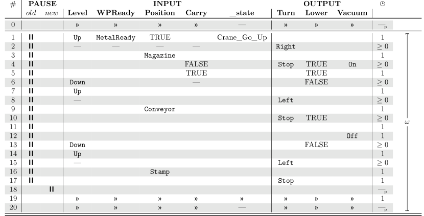
Figure 6: Combination of regression and delta verification. For presentation reason, we omitted trace reference in the column header. All columns belonging to the $new$ trace.

Scenario

In this scenario, we demonstrate a combination of regression verification and delta verification [14] for two software revisions. While regression verification proves the equivalence for the common part of system behaviour, delta verification ensures functional correctness for the differences. This scenario is based on the evolution step from the third to the fifth software revision of the PPU, which introduces an optimisation for work piece throughput: The new software revision makes use of the waiting time while a piece is stamped to deliver a new work piece from the magazine to the conveyor belt. The old revision waits for the stamp to finishing the imprint.

Table

The rtt in Fig. 6 contains rows for the following input and output variables: (a) Levelindicating the position of the crane (Up, Down, Unknown), (b) WPReadysignalling whether a (non-)metal work piece is ready at the magazine, (c) Positionof the crane (Magazine, Stamp, etc.), (d) Carrysignalling whether a work piece has been picked up, (e) the current _state of the internal state machine, (f) Turndetermining the move direction of the crane (Stop, Left, Right), (g) the desired position of the suction cup (Lower), and (h) whether the suction cup should hold a work piece. The table specifies that the $\mathit{old}$ (third) revision and the $\mathit{new}$ (fifth) revision behave equally (Row 0, Row 19, Row 20), except for the phase in which the optimisation is occurs. During the optimisation phase, the trace of the $\mathit{old}$ revision stutters (Row 1 to 17) while the $\mathit{new}$ trace moves the crane to the magazine, picks up the work piece, delivers it to the conveyor belt, and moves the crane back to the stamp. This sequence is described as a functional specification. In Row 18, we pause the $\mathit{new}$ trace and let the $\mathit{old}$ trace run until both traces are synchronised again on the same internal state $\_state$. This is required, because the waiting duration for imprinting is hard-coded and cannot be changed.

Verification

We proved system conformance to the rtt for the function block of Crane module, resulting into a product program with 726 lines of code and 72 variables. Verification of weak conformance took 5.66 seconds with a state size of 209 bits (software and table). For the verification we decreased the waiting durations of the timers.

5.2 Information Flow

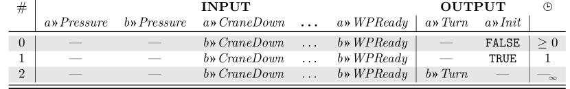
Figure 7: Information-flow property: the input $\mathit{Pressure}$ should not have an influence on the output $\mathit{Turn}$.

Scenario and Table

In this scenario, we verify that there is no information flow from the suction pressure ($\mathit{Pressure}$) to the crane movement ($\mathit{Turn}$). More precisely, the table in Fig. 7 describes that the non-interference is only required after the initialisation of the system (Row 2, $\mathit{Init}$). In all rows, we enforce that all input variables besides $\mathit{Pressure}$ are equal in both runs. Row 2 expresses the non-interference property: For any two runs with arbitrary values for $\mathit{Pressure}$, the output $\mathit{Turn}$ is the same. Therefore, $\mathit{Turn}$ is only determined by the other input variables.

Unfortunately, a monitor function block stops the crane if the suction pressure is outside the expected range, i.e., if $\mathit{Pressure}\not\in[1,9999]$. Therefore, the software does in fact not conform to the rtt in Fig. 7. This unintended outcome can be fixed by limit the (unknown) values of $\mathit{Pressure}$ in both traces to the range $[1,9999]$.

Verification

We used the complete fifth revision of the PPU, including the function blocks for all components. The product program has 1758 lines of code with 266 variables. For the interfering version, the model checker needs 25.93 seconds to find a counter example. Proving conformance w.r.t. the fixed – non-interfering – specification takes 122.26 seconds. The size of the state space is 373 bits.

6 Conclusion

In this paper, we have presented rtts, a canonical extension of the gtt concept for the specification of relational properties for reactive systems. The semantics of rtt is defined by reduction to that of gtts, whereas the syntax is a genuine extension to gtts. For future work, the next step is the adaption of time synchronisation points to increase the flexibility between traces. For example, allowing the specification of parallel runs with all possible interleavings.

References

- [1] Barthe, G., D’Argenio, P.R., Rezk, T.: Secure information flow by self-composition. In: Proceedings. 17th IEEE Computer Security Foundations Workshop, 2004. pp. 100–114 (June 2004)
- [2] Barthe, G., Eilers, R., Georgiou, P., Gleiss, B., Kovács, L., Maffei, M.: Verifying relational properties using trace logic. CoRR abs/1906.09899 (2019), http://arxiv.org/abs/1906.09899
- [3] Beckert, B., Cha, S., Ulbrich, M., Vogel-Heuser, B., Weigl, A.: Generalised test tables: A practical specification language for reactive systems. In: Polikarpova, N., Schneider, S. (eds.) Integrated Formal Methods. pp. 129–144. Springer International Publishing, Cham (2017)
- [4] Beckert, B., Ulbrich, M., Vogel-Heuser, B., Weigl, A.: Regression verification for programmable logic controller software. In: 17th International Conference on Formal Engineering Methods (ICFEM 2015). LNCS, vol. 9407, pp. 234–251. Springer (Dec 2015)
- [5] Blatter, L., Kosmatov, N., Gall, P.L., Prevosto, V.: Deductive verification with relational properties. ArXiv abs/1606.00678 (2016)
- [6] Bradley, A.R., Manna, Z.: Checking safety by inductive generalization of counterexamples to induction. In: Formal Methods in Computer Aided Design, 2007. FMCAD ’07. pp. 173–180 (Nov 2007)
- [7] Cavada, R., Cimatti, A., Dorigatti, M., Griggio, A., Mariotti, A., Micheli, A., Mover, S., Roveri, M., Tonetta, S.: The nuXmv symbolic model checker. In: Computer Aided Verification (CAV). pp. 334–342. LNCS 8559, Springer (2014)
- [8] Clarkson, M.R., Finkbeiner, B., Koleini, M., Micinski, K.K., Rabe, M.N., Sánchez, C.: Temporal logics for hyperproperties. In: Abadi, M., Kremer, S. (eds.) Principles of Security and Trust - Third International Conference, POST 2014, Held as Part of the European Joint Conferences on Theory and Practice of Software, ETAPS 2014, Grenoble, France, April 5-13, 2014, Proceedings. Lecture Notes in Computer Science, vol. 8414, pp. 265–284. Springer (2014), https://doi.org/10.1007/978-3-642-54792-8_15
- [9] Clarkson, M.R., Schneider, F.B.: Hyperproperties. Journal of Computer Security 18(6), 1157–1210 (2010)
- [10] Denning, D.E.: A lattice model of secure information flow. Commun. ACM 19(5), 236–243 (May 1976), http://doi.acm.org/10.1145/360051.360056
- [11] Felsing, D., Grebing, S., Klebanov, V., Rümmer, P., Ulbrich, M.: Automating regression verification. In: Crnkovic, I., Chechik, M., Grünbacher, P. (eds.) ACM/IEEE International Conference on Automated Software Engineering, ASE ’14, Vasteras, Sweden - September 15 - 19, 2014. pp. 349–360. ACM (2014), http://doi.acm.org/10.1145/2642937.2642987
- [12] Pakonen, A., Pang, C., Buzhinsky, I., Vyatkin, V.: User-friendly formal specification languages – conclusions drawn from industrial experience on model checking. In: IEEE International Conference on Emerging Technologies and Factory Automation (ETFA 2016). Berlin, Germany (2016)
- [13] Scheben, C., Schmitt, P.H.: Efficient self-composition for weakest precondition calculi. In: Jones, C.B., Pihlajasaari, P., Sun, J. (eds.) FM 2014: Formal Methods - 19th International Symposium, Singapore, May 12-16, 2014. Proceedings. Lecture Notes in Computer Science, vol. 8442, pp. 579–594. Springer (2014), https://doi.org/10.1007/978-3-319-06410-9_39
- [14] Ulewicz, S., Ulbrich, M., Weigl, A., Kirsten, M., Wiebe, F., Beckert, B., Vogel-Heuser, B.: A verification-supported evolution approach to assist software application engineers in industrial factory automation. In: IEEE International Symposium on Assembly and Manufacturing (ISAM). pp. 19–25. Fort Worth, USA (2016)
- [15] Vogel-Heuser, B., Legat, C., Folmer, J., Feldmann, S.: Researching Evolution in Industrial Plant Automation: Scenarios and Documentation of the Pick and Place Unit. Tech. Rep. TUM-AIS-TR-01-14-02 (2014), https://mediatum.ub.tum.de/doc/1208973/1208973.pdf
- [16] Yi, J., Qi, D., Tan, S.H., Roychoudhury, A.: Software change contracts. ACM Trans. Softw. Eng. Methodol. 24(3), 18:1–18:43 (2015), http://doi.acm.org/10.1145/2729973