Improved solution to data gathering with mobile mule

Abstract

In this work we study the problem of collecting protected data in ad-hoc sensor network using a mobile entity called MULE. The objective is to increase information survivability in the network. Sensors from all over the network, route their sensing data through a data gathering tree, towards a particular node, called the sink. In case of a failed sensor, all the aggregated data from the sensor and from its children is lost. In order to retrieve the lost data, the MULE is required to travel among all the children of the failed sensor and to re-collect the data. There is a cost to travel between two points in the plane. We aim to minimize the MULE traveling cost, given that any sensor can fail. In order to reduce the traveling cost, it is necessary to find the optimal data gathering tree and the MULE location. We are considering the problem for the unit disk graphs (UDG) and Euclidean distance cost function. We propose a primal-dual algorithm that produces a $\left(20+\varepsilon\right)$-approximate solution for the problem, where $\varepsilon\rightarrow 0$ as the sensor network spreads over a larger area. The algorithm requires $O\left(n^{3}\cdot\varDelta\left(G\right)\right)$ time to construct a gathering tree and to place the MULE, where $\varDelta\left(G\right)$ is the maximum degree in the graph and $n$ is the number of nodes.

Keywords: WSN $\cdot$ MULE $\cdot$ MWCDS $\cdot$ Primal-Dual $\cdot$ UDG

1 Introduction

Consider an Ad-Hoc sensor network randomly embedded in the plane. An example application is the use of sensors scattered in forests using aircraft, to give an indication when a fire starts. The main problem in WSN is long-term survivability. Because of the limited energy of the sensor, its lifetime depends on its energy consumption. A standard solution for efficient utilization of energy is to build a data gathering tree in the network. In this method, the data is aggregated in order to reduce the number of messages each sensor transmits. The sensors create a logical construction of a tree in the network, and all the data routed to the sink according to that tree. The basic principle of the data aggregation is that each sensor waits to aggregate the data from all its children before it sends its own message to its father. When a sensor failure occurs, all the aggregated data from the sensor and its children are lost. Also, if the sensor is not a leaf in the tree, its entire subtree is disconnected. It takes a long time to recognize the fault, and for the network to reconstruct a new gathering tree. Here comes the use of data MULE to retrieve the lost data. Data MULE is a mobile unit provided with extended computing and storage capabilities, and short-range wireless communication.

In order to gather data from the children of a failed sensor, the MULE should travel and approach each child. After visiting all of the children, the MULE returns to its starting point. There is a cost to travel between two points. Given a graph of gathering sensors network, we would like to find the data gathering tree and the position of the MULE, which minimizes the traveling cost, while each sensor could fail. It is common to model wireless sensor networks as a Unit Disk Graph (UDG), where the transmission range of the sensors is defined as one unit. The sensors are the nodes, and between each pair of sensors that can communicate directly with each other, there will be an edge in the graph. The MULE problem was previously defined by Crowcroft et al. [3] and Yedidsion et al. [14].

In this work, we focused primarily on the study of the problem on general unit disk graphs for Euclidean distance cost function, and only one sensor can fail at a time.

The paper is organized as follows. In the next section we present the previous related work. In Section 3 we define our problem and model, and introduce the main subjects that our method is based on. In Section 4 we show reductions of the problem which we use later. We present our algorithm and analyze its performance, in Section 5. In Section 6 we present simulation results of our algorithm, and conclude in Section 7.

2 Related work

In the last years, some research has been started to evaluate how Data MULEs can benefit the performance of wireless sensor networks. Two major approaches have developed in this area. The first approach is the regular use of data MULEs in order to pass data between remote components in the network [10, 8, 11]. The second approach is using data MULEs in order to increase information survivability in the network. The main idea is to use MULEs to amend failures in the network. This is where our work takes place. Crowcroft et al. [3] use this approach to deal with the problem of efficient data recovery using the data MULEs approach. They consider a sensor network that uses a data gathering tree. The main idea is to use MULEs in order to retrieve lost data caused by failed sensors by visiting the children of the failed sensors. They define the problem as “$(\alpha,\beta)-Mule$”, when $\alpha$ is the amount of simultaneously failed sensors and $\beta$ is the number of MULEs in the network. They study several aspects of the problem and suggest a variety of solutions to the problem on the following graph topologies: complete graph and UDG (line, random line, and grid). Yedidsion et al. [14] also study the same problem of data gathering in sensor networks using MULE. They consider the problem when there is one MULE in the network, and only one sensor can fail at the same time. They study the problem for several topologies, such as UDG on a line and general UDG. Further, they also consider a failure probability for each sensor and study the problem for a complete graph. For the UDG on a line, they present an $O\left(n\right)$ time algorithm that solves the problem. For a general UDG graph, they present an algorithm and two approaches to analyze its approximation ratio, with a tradeoff between runtime and approximation. The first approach achieves $\left(57+\epsilon\right)$ approximation and takes $O\left(n^{3}\log n\right)$ time, where $\epsilon$ comes from a TSP calculation (according to [9]) for the approximation ratio. The second approach reduces operations and achieves $O\left(n^{2}\log n\right)$ time. However, it pays with a worse approximation of $\left(114+\epsilon\right)$. Ashur [1] continued their study on a general UDG, and came up with a very large constant-factor approximation algorithm for the problem, which requires $O\left(n\log n\right)$ runtime.

Like Yedidsion et al. [14] and Ashur [1], we will also focus on the MULE problem for a general UDG graph, when there is one MULE, and only one sensor can fail at a time. We use a different approach to solve the problem, and propose a primal-dual algorithm that achieves a $\left(20+\varepsilon\right)$-approximation for the MULE problem but has a higher runtime of $O\left(n^{3}\cdot\varDelta\left(G\right)\right)$. We note that $\varDelta\left(G\right)$ is the maximum degree in the graph, $n$ is the number of nodes, and $\varepsilon\rightarrow 0$ as the sensor network spreads over a larger area.

3 Preliminaries and Model

3.1 Problem definition

Definition 1 (Data gathering tree).

Data gathering tree $T=\left(V,E_{T}\right)$ is a directed spanning tree in graph $G=\left(V,E\right)$. Consider a spanning tree in $G$ and a root node $r$, $T$ is the rooted directed version of the spanning tree, where from each node in the tree there is a directed path to $r$.

In this work, we study the MULE problem for UDG, where there is one MULE and only one sensor failure at a time, in the network. We will refer to this problem as “$\left(1,1\right)-MULE-UDG$”, and it is defined as follows: Consider a network of sensors embedded in the plane with the same transmission range. Let $G=\left(V,E\right)$ be a connected UDG that models the WSN, when the sensors are nodes, and an edge is defined between a pair of nodes only if they are within the transmission range of each other. Let $T$ be a data gathering tree which spans all the nodes in $G$. $T$ is rooted at node $r$, and sensing data propagates from leaf nodes to the root. One MULE is located at some node on the graph. Let $m$ be the MULE location. The MULE can travel between a set of nodes, where the cost function of a tour $t$ (referred to as $c\left(t\right)$) is its total Euclidean distances. Let $\delta\left(v,T\right)$ be the set of children that $v$ has in tree $T$. When sensor $v_{f}$ fails, all data gathered from its children is lost, and the MULE must travel through all of its children, in order to retrieve the lost data. The MULE performs a circular tour that goes through all the nodes $\delta\left(v_{f},T\right)$ and at the end returns to the starting position $m$. Let $t\left(m,\delta\left(v_{f},T\right)\right)$ be the shortest circular tour through all the nodes in $\left\{m\right\}\cup\delta\left(v_{f},T\right)$, that the MULE has to take. The objective will be to minimize the overall MULE tour, regardless of which sensor fails. Formally, the problem is defined as follows:

Definition 2 ($\left(1,1\right)-MULE-UDG$ problem).

Given a connected UDG graph denoted by $G=\left(V,E\right)$, our goal is to find the MULE location $m$ and the data gathering tree $T$, which minimizes the objective function:

$$\min_{m,T}\left[\sum_{v_{f}\in V}\left[c\left(t\left(m,\delta\left(v_{f},T\right)\right)\right)\right]\right]\;.$$

3.2 The primal-dual method

The field of combinatorial optimization problems has been heavily influenced by the field of Linear Programming (LP) since many combinatorial problems can be described as linear programming problems. The primal-dual method was first introduced by Dantzig, Ford, and Fulkerson [4] in 1956, in order to find an exact solution for linear programming problems. The principle of the primal-dual method can also be useful for finding an approximate solution in polynomial time for NP-hard optimization problems, and this method is called “The Primal-Dual Method for Approximation Algorithms”. The main idea is to construct a feasible solution for the LP problem (referred as the “Primal LP Problem”) from scratch, using a related LP problem (referred as the “Dual LP Problem”) that guides us during the construction of the feasible solution. In our case, the relationship between the primal and the dual problems is such that, the primal solution serves as an upper bound, while the dual solution serves as a lower bound for the optimal solution OPT. The performance of a primal-dual approximation algorithm is measured by the ratio between the primal and the dual solutions it finds. In 1995, Goemans and Williamson [6] proposed a general technique for designing approximation algorithms based on this method. Their technique produces 2-approximation algorithms for a broad set of graph problems that run in $O\left(n^{2}\log n\right)$ time. Their technique had a significant impact on our research. For more details about the primal-dual method, we will refer the reader to the papers [6, 12, 7].

3.3 Minimum-weighted connected dominating set problem

For a later use, we want to define the term MIS and the problem of MWCDS.

Given a graph $G=\left(V,E\right)$, a set $S\subseteq V$ will be called an Independent Set (IS), if for each pair of nodes $u,v\in S$ there is no edge $\left(u,v\right)\in E$. The set will also be called a Maximal Independent Set (MIS), if it is an IS and there is no node $v\in V\setminus S$ which can be added to the set while it will still remain independent.

Consider the graph $G=\left(V,E\right)$, a set of nodes $S\subseteq V$ will be called a Dominating Set (DS), if each node $v\in V$ is either in the set or is a neighbor of any node in the set. The DS with the minimum cardinality is called a Minimum Dominating Set (MDS). A set of nodes $S\subseteq V$ will be called Connected Set (CS) if its induced graph in $G$ is connected. A set of nodes $S\subseteq V$ will be called Connected Dominating Set (CDS) if $S$ is both dominating set and connected. The CDS with the minimum cardinality is called a Minimum Connected Dominating Set (MCDS). Consider a weight function for each node in graph $G$, the DS with the minimum total node weights is called a Minimum-Weighted Dominating Set (MWDS) and the CDS with the minimum total node weights is called a Minimum-Weighted Connected Dominating Set (MWCDS).

Definition 3 (MWCDS problem).

Given a connected graph denoted by $G=\left(V,E\right)$ and a node weight function $w\left(v\right)\vcentcolon V\rightarrow R^{+}$, our goal is to find a subset of nodes $S\subseteq V$, which is CDS in $G$ and minimizes the objective function:

$$\min_{S\subseteq V}\left\{\sum_{v\in S}w\left(v\right)\right\}\;.$$

Finding MCDS is an NP-complete problem for UDG ([2]). Hence the more general case of MWCDS is also an NP-complete problem. In 2010 Erlebach and Matus [5] presented a polynomial-time algorithm that achieves approximation of $\left(4+\epsilon\right)$ for MWDS, and they combine it with a known algorithm for node-weighted Steiner trees to achieve a $7.875$-approximation for MWCDS in UDG graphs. In addition, independently, in 2011 Zou et al. [15] also introduced a polynomial-time algorithm that achieves $\left(4+\varepsilon\right)$-approximation to the MWDS problem on UDG. Due to the method they were based on, there is a trade-off between the approximation performance ratio and the runtime. So they only proved that the runtime was polynomial, but they did not analyze it accurately.

We wanted to put more emphasis on a reasonable runtime, and therefore in this work, we chose to use a different method than the others: we will use the Primal-Dual method.

4 Reduction of The Problem

4.1 Reduction to an approximate MWCDS problem

The MULE problem we study seems to be an NP-hard problem, although it has not yet been proven. It is interesting to note that with some reasonable assumptions, the $\left(1,1\right)-MULE-UDG$ problem can be reduced to the problem of finding a MWCDS, when the node weight is proportional to its Euclidean distance from the MULE. We assume that the MULE has a fixed transmission range of $R_{M}$, within the range $0<R_{M}<0.3\cdot R$, where $R$ is the sensor’s transmission range. In our case, for UDG, $R=1$ and the range will be $0<R_{M}<0.3$. In other words, the MULE does not need to reach the exact location of the sensor, but it needs to get close enough to communicate with it.

Let $m$ be any location of the MULE, and $T$ be some gathering tree. The MULE’s tour for a failure $t\left(m,\delta\left(v,T\right)\right)$ of node $v$ can be represented as a series of nodes according to their order $\left\{m,u_{1},u_{2},u_{3},\ldots,u_{\left|\delta\left(v,T\right)\right|},m\right\}$. We will consider the tour as three separate parts. $LWF\left(v,T\right)$ (“Long Walk Forward”) is the cost of the MULE’s walk from node $m$ to node $u_{1}$, for the failure of node $v$ in gathering tree $T$. $LWB\left(v,T\right)$ (“Long Walk Backward”) is the cost of the MULE’s walk from node $u_{\left|\delta\left(v,T\right)\right|}$ to node $m$. $WAC\left(v,T\right)$ (“Walking Among Children”) is the cost of the MULE’s walk from node $u_{1}$ to node $u_{\left|\delta\left(v,T\right)\right|}$, through the rest of $v$’s children $u_{2},u_{3},\ldots,u_{\left|\delta\left(v,T\right)\right|-1}$ in tree $T$.

Let $Cost\left(T,m\right)$ be the total tours cost $\sum_{v_{f}\in V}c\left(t\left(m,\delta\left(v_{f},T\right)\right)\right)$ for a MULE located at $m$ and for gathering tree $T$. Let us denote the BackBone ($BB$) of gathering tree $T$ to be the induced undirected subgraph of $T$, which contains all the non-leaf nodes, that is, all nodes with degree greater than one. The BackBone is denoted by $T_{BB}=\left(V_{BB},E_{BB}\right)$, where $V_{BB}$ is the set of the BackBone’s nodes and $E_{BB}$ is its set of edges. Let $OPT_{T^{\ast}}$ be the cost of the optimal solution for the $\left(1,1\right)-MULE-UDG$ problem, and $m^{\ast}$ be the optimal MULE location, where $T^{\ast}=\left(V,E_{T}^{\ast}\right)$ is the data gathering tree of the solution. That is, $OPT_{T^{\ast}}=Cost\left(T^{\ast},m^{\ast}\right)$. Let $V_{BB}^{\ast}$ be the BackBone nodes of $T^{\ast}$. We denote by $dist\left\{m,v\right\}$ the Euclidean distance between node $v$ and the MULE location $m$.

Proposition 4.

If we consider the MULE’s transmission range as a constant in the range $0<R_{M}<0.3$, then for any data gathering tree $T$ and for each node $v\in V$, we can bound $WAC\left(v,T\right)\leq C_{1}$, where $C_{1}=\left(1+R_{M}\right)\left(1+\pi\left(1+\left\lceil\nicefrac{{\left(1-R_{M}\right)}}{{2R_{M}}}\right\rceil\right)\right)$.

Proof.

Note that all the children of any node are scattered over a fixed area due to the UDG property, a disk area of radius $1$ (i.e. the node transmission area). One extreme possibility for the MULE’s tour will be to reach a failed node with precisely one child. In this case, the MULE has no need to walk in the transmission area around the node, and therefore we have $WAC\left(v,T\right)=0$. As the nodes density increases in the graph, the children of a node are increasingly filling the transmission area around it, and the MULE will have to walk a lot more to reach all of them. Therefore, the extreme case on the other side will be when the MULE has to walk all over the transmission area of the failed node, in order to reach all of its children. Since we assumed that the MULE has a fixed transmission range $R_{M}$, we want to show that there is a fixed-length walk during which the MULE approaches each child at a distance of $R_{M}$.

The description of the walk is as follows. First, the MULE reaches the center of the area, where the failed node is located. From there, it moves in increasing circles, until full coverage of the area (as described in Figure 1). The first circle is with radius $2R_{M}$, and for all the rest, each circle has a radius that grows by $2R_{M}$ from its predecessor. Each time the MULE completes an entire circle, it moves $2R_{M}$ units away in the direction of the radius and starts the walk of the next circle. In order to cover the whole transmission area, the amount of circles required is $\left\lceil\nicefrac{{\left(R-R_{M}\right)}}{{2R_{M}}}\right\rceil$.

Calculating the total length of the MULE walk consists of walking in circles $\sum_{i=1}^{\left\lceil\nicefrac{{\left(R-R_{M}\right)}}{{2R_{M}}}\right\rceil}2\pi\cdot\left(i\cdot 2R_{M}\right)$ and walking between circuits $\left\lceil\nicefrac{{\left(R-R_{M}\right)}}{{2R_{M}}}\right\rceil\cdot 2R_{M}$. Let us define $N_{R}\triangleq\left\lceil\nicefrac{{\left(R-R_{M}\right)}}{{2R_{M}}}\right\rceil$, we get:

$$\begin{array}[]{rl}WAC\left(v,T\right)\leq&N_{R}\cdot 2R_{M}+\sum_{i=1}^{N_{R}}2\pi\cdot\left(i\cdot 2R_{M}\right)\\ =&N_{R}\cdot 2R_{M}+\frac{N_{R}}{2}\left(2\pi\cdot 2R_{M}+2\pi\cdot N_{R}\cdot 2R_{M}\right)\\ =&2R_{M}\cdot N_{R}\left(1+\pi\left(1+N_{R}\right)\right)\\ =&2R_{M}\cdot\left\lceil\nicefrac{{\left(R-R_{M}\right)}}{{2R_{M}}}\right\rceil\left(1+\pi\left(1+\left\lceil\nicefrac{{\left(R-R_{M}\right)}}{{2R_{M}}}\right\rceil\right)\right)\\ \leq&\left(1+R_{M}\right)\left(1+\pi\left(1+\left\lceil\nicefrac{{\left(1-R_{M}\right)}}{{2R_{M}}}\right\rceil\right)\right)\\ =&C_{1}\;.\end{array}$$

The second inequality derives from the rounding up operation and since $R=1$. ∎

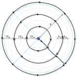
Figure 1: Bounded walk among children of a failed sensor.

Lemma 5.

Let $\left(2\cdot dist\left\{m,v\right\}+C\right)$ be the weight of node $v$, where $C$ is a positive constant dependent on $R_{M}$. Then $Cost\left(T,m\right)$ can be bounded from above by the total weight of $T^{\prime}s$ BackBone nodes.

Proof.

Since a leaf node has no children in the tree $T$, the MULE does not go on tour for the failure of a leaf node. Therefore, the only nodes for which the tour cost $c\left(t\left(m,\delta\left(v_{f},T\right)\right)\right)$ is greater than $0$ are the BackBone nodes of $T$. So, we can write:

$$Cost\left(T,m\right)\triangleq\sum_{v_{f}\in V}c\left(t\left(m,\delta\left(v_{f},T\right)\right)\right)=\sum_{v\in V_{BB}}c\left(t\left(m,\delta\left(v,T\right)\right)\right)\;.$$ (1)

The MULE’s tour consists of $3$ different walks, $LWF\left(v,T\right)$, $LWB\left(v,T\right)$ and $WAC\left(v,T\right)$. Note that from the triangle inequality, and since a child of node $v$ can be at most one unit away from $v$, we get: $LWF\left(v,T\right)\leq dist\left\{m,v\right\}+1$ and $LWB\left(v,T\right)\leq dist\left\{m,v\right\}+1$. Combining this with Proposition 4, we will get:

$$\begin{array}[]{rl}c\left(t\left(m,\delta\left(v,T\right)\right)\right)=&LWF\left(v,T\right)+WAC\left(v,T\right)+LWB\left(v,T\right)\\ \leq&\left(dist\left\{m,v\right\}+1\right)+C_{1}+\left(dist\left\{m,v\right\}+1\right)\\ =&2\cdot dist\left\{m,v\right\}+2+C_{1}\;.\end{array}$$ (2)

Let us define $C\triangleq 2+C_{1}$. Thus, in conclusion:

$$\begin{array}[]{rl}Cost\left(T,m\right)\stackrel{{\scriptstyle\left(\ref{eq:T-R-P-2}\right)}}{{=}}&\sum_{v\in V_{BB}}c\left(t\left(m,\delta\left(v,T\right)\right)\right)\\ \stackrel{{\scriptstyle\left(\ref{eq:T-R-P-3}\right)}}{{\leq}}&\sum_{v\in V_{BB}}\left(2\cdot dist\left\{m,v\right\}+C\right)\;,\end{array}$$ (3)

where, $C=3+R_{M}+\pi\left(1+R_{M}\right)\left(1+\left\lceil\nicefrac{{\left(1-R_{M}\right)}}{{2R_{M}}}\right\rceil\right)$ (Figure 2). ∎

Figure 2: Constant $C$ as a function of $R_{M}$.

Lemma 6.

Let $\left(2\cdot dist\left\{m,v\right\}-2.6\right)$ be the weight of node $v$. Then $Cost\left(T,m\right)$ can be bounded from below by the total weight of $T^{\prime}s$ BackBone nodes.

Proof.

Note that the shortest tour to a particular failed node $v$ is in case the node has exactly one child in $T$, which is located as close as possible to the MULE. Since this is only one child, then $WAC\left(v,T\right)=0$. We will distinguish between two possible cases: when the MULE is located within the transmission area of the failed node $v$, and when it is located outside it. In the first case, $dist\left\{m,v\right\}\leq 1$ and the shortest possible tour will have a cost of $0$ (in case the MULE is located such that the only child is within its transmission range). So we have $LWF\left(v,T\right)=LWB\left(v,T\right)=0\geq dist\left\{m,v\right\}-1.3$. In the second case, where $dist\left\{m,v\right\}>1$, the location of the child that minimizes its distance from the MULE will be directly between the node $v$ and the MULE, at the edge of $v$’s transmission range (exactly one unit away from $v$). This implies that $LWF\left(v,T\right)=LWB\left(v,T\right)=dist\left\{m,v\right\}-1-R_{M}$. Recall that $R_{M}<0.3$. Therefore we can bound the MULE’s tour from below, as follows:

$$c\left(t\left(m,\delta\left(v,T\right)\right)\right)=LWF\left(v,T\right)+WAC\left(v,T\right)+LWB\left(v,T\right)>2\cdot\left(dist\left\{m,v\right\}-1.3\right)\;.$$ (4)

Combine it with Equation 1 of Lemma 5, we get:

$$Cost\left(T,m\right)\stackrel{{\scriptstyle\left(\ref{eq:T-R-P-2}\right)}}{{=}}\sum_{v\in V_{BB}}c\left(t\left(m,\delta\left(v,T\right)\right)\right)\stackrel{{\scriptstyle\left(\ref{eq:T-R-P-5}\right)}}{{>}}\sum_{v\in V_{BB}}\left(2\cdot dist\left\{m,v\right\}-2.6\right)\;.$$

∎

Theorem 7.

Consider the optimal solution for the MWCDS problem [3] for node weights $\left(2\cdot dist\left\{m^{\ast},v\right\}+C\right)$, where $C$ is a positive constant dependent on $R_{M}$ and $m^{\ast}$ is the optimal MULE location for the $\left(1,1\right)-MULE-UDG$ problem. Let $V_{BB}^{\ast}$ be the BackBone nodes of the optimal gathering tree. If the condition $\underset{v\in V_{BB}^{\ast}}{Average}\left[dist\left\{m^{\ast},v\right\}\right]>1.3$ is met, then a data gathering tree whose BackBone consists of the optimal solution to this specific MWCDS problem is an $\left(1+\varepsilon\right)$-approximate solution for the $\left(1,1\right)-MULE-UDG$ problem, where as the area of the BackBone increases, the smaller the $\varepsilon$ (i.e. $\varepsilon\rightarrow 0$ for $\underset{v\in V_{BB}^{\ast}}{Average}\left[dist\left\{m^{\ast},v\right\}\right]\rightarrow\infty$).

Proof.

We will denote $OPT_{cds^{\ast}}$ to be the total weight of the optimal solution for the MWCDS problem, where $cds^{\ast}$ is the optimal CDS itself, which achieves this weight. If the nodes weights are $\left(2\cdot dist\left\{m^{\ast},v\right\}+C\right)$, then according to the problem definition [3], we have:

$$OPT_{cds^{\ast}}=\sum_{v\in cds^{\ast}}\left(2\cdot dist\left\{m^{\ast},v\right\}+C\right)\;.$$ (5)

From the other side, of the $\left(1,1\right)-MULE-UDG$ problem, let us define the weight of a gathering tree $T$ (referred as $Weight_{BB}\left(T\right)$), to be the total weight of its BackBone nodes.

We want to claim that the BackBone of $T$ is a CDS. Therefore we are required to show that the BackBone is both dominating and connected. $T$ is a spanning tree in $G$ by definition [1]. Thus, it is connected and contains all the nodes. Since $T$ is connected, each node in $T$ is either a leaf or a BackBone node, and if it is a leaf, then it has a neighbor in the BackBone. So, the BackBone is a DS. $T$ is connected by definition [1]. Therefore, if we will prune all of its leaves it will still remain connected. Hence, the BackBone nodes are also a CDS.

We assume that the root node is not a leaf. Otherwise, we can always replace $T^{\ast}$ with such a tree, without affecting the approximation ratio. Let $r$ and $v$ be the root node and one of its neighbors, respectively. If $r$ is a leaf, we can replace $v$ to be the root instead. Thus we will create a new tree $T^{\prime}$, for which $LWF\left(v,T^{\prime}\right)=LWB\left(v,T^{\prime}\right)=0$ and $WAC\left(v,T^{\prime}\right)\leq WAC\left(v,T^{\ast}\right)+4$. The worst case of adding $4$ to the total tour cost of $T^{\prime}$ does not affect the approximation ratio.

The BackBone nodes of $T$ is a CDS, and the root is one of these nodes. If the total weight of the BackBone is the weight of the tree, then it can be said that, finding a tree with the lowest weight is equivalent to finding a MWCDS in the graph. Formally, the following equality holds:

$$\begin{array}[]{rl}\min\limits_{T}\left\{Weight_{BB}\left(T\right)\right\}=&\min\limits_{T}\left\{\sum\limits_{v\in V_{BB}}\left(2\cdot dist\left\{m^{\ast},v\right\}+C\right)\right\}\\ \begin{array}[]{c}=\\ \\ \end{array}&\begin{array}[]{l}\min\limits_{S\subseteq V}\left\{Weight\left(S\right)\right\}\\ s.t\>S\>is\>a\>CDS\end{array}\\ =&\sum\limits_{v\in cds^{\ast}}\left(2\cdot dist\left\{m^{\ast},v\right\}+C\right)\;.\end{array}$$ (6)

A gathering tree with the lowest weight has a lower weight than any other tree, in particular $T^{\ast}$. Note that these are not necessarily the same gathering trees. Therefore:

$$\begin{array}[]{rl}\min\limits_{T}\left\{Weight_{BB}\left(T\right)\right\}=&\min\limits_{T}\left\{\sum\limits_{v\in V_{BB}}\left(2\cdot dist\left\{m^{\ast},v\right\}+C\right)\right\}\\ \leq&Weight_{BB}\left(T^{\ast}\right)\\ =&\sum\limits_{v\in V_{BB}^{\ast}}\left(2\cdot dist\left\{m^{\ast},v\right\}+C\right)\;.\end{array}$$ (7)

From Lemma 5 and Lemma 6 we have seen that $OPT_{T^{\ast}}$ can be bounded as follows:

$$\sum_{v\in V_{BB}^{\ast}}\left(2\cdot dist\left\{m^{\ast},v\right\}-2.6\right)<OPT_{T^{\ast}}\leq\sum_{v\in V_{BB}^{\ast}}\left(2\cdot dist\left\{m^{\ast},v\right\}+C\right)\;.$$

Now, we will calculate how much the upper bound is greater than the optimal solution.

$$\begin{array}[]{rl}\frac{\sum_{v\in V_{BB}^{\ast}}\left(2\cdot dist\left\{m^{\ast},v\right\}+C\right)}{OPT_{T^{\ast}}}<&\frac{\sum_{v\in V_{BB}^{\ast}}\left(2\cdot dist\left\{m^{\ast},v\right\}+C\right)}{\sum_{v\in V_{BB}^{\ast}}\left(2\cdot dist\left\{m^{\ast},v\right\}-2.6\right)}\\ =&\frac{\sum_{v\in V_{BB}^{\ast}}2\cdot dist\left\{m^{\ast},v\right\}+\left|V_{BB}^{\ast}\right|C}{\sum_{v\in V_{BB}^{\ast}}2\cdot dist\left\{m^{\ast},v\right\}-\left|V_{BB}^{\ast}\right|2.6}\\ =&1+\frac{1}{\frac{2}{\left(C+2.6\right)}\cdot\left(\frac{\sum_{v\in V_{BB}^{\ast}}dist\left\{m^{\ast},v\right\}}{\left|V_{BB}^{\ast}\right|}-1.3\right)}\\ =&1+\frac{1}{\frac{2}{\left(C+2.6\right)}\cdot\left(\underset{v\in V_{BB}^{\ast}}{Average}\left[dist\left\{m^{\ast},v\right\}\right]-1.3\right)}\\ =&1+\varepsilon\;,\end{array}$$ (8)

where, $\varepsilon\triangleq\left(\frac{2}{\left(C+2.6\right)}\cdot\left(\underset{v\in V_{BB}^{\ast}}{Average}\left[dist\left\{m^{\ast},v\right\}\right]-1.3\right)\right)^{-1}$, and hence $\varepsilon\rightarrow 0$ for $\underset{v\in V_{BB}^{\ast}}{Average}\left[dist\left\{m^{\ast},v\right\}\right]\rightarrow\infty$. That is, the $\varepsilon$ error decreases as the average distance of the BackBone nodes from the MULE, increases. Also, as the graph will be deployed over a wider area. We should note that for correct approximation, the condition $\underset{v\in V_{BB}^{\ast}}{Average}\left[dist\left\{m^{\ast},v\right\}\right]>1.3$ must be met.

Finally, we will summarize everything in one equation:

$$\begin{array}[]{rl}OPT_{cds^{\ast}}\stackrel{{\scriptstyle\left(\ref{eq:T-R-P-7}\right)}}{{=}}&\sum_{v\in cds^{\ast}}\left(2\cdot dist\left\{m^{\ast},v\right\}+C\right)\\ \stackrel{{\scriptstyle\left(\ref{eq:T-R-P-8}\right)}}{{=}}&\min\limits_{T}\left\{\sum_{v\in V_{BB}}\left(2\cdot dist\left\{m^{\ast},v\right\}+C\right)\right\}\\ \stackrel{{\scriptstyle\left(\ref{eq:T-R-P-9}\right)}}{{\leq}}&\sum_{v\in V_{BB}^{\ast}}\left(2\cdot dist\left\{m^{\ast},v\right\}+C\right)\\ \stackrel{{\scriptstyle\left(\ref{eq:T-R-P-10}\right)}}{{<}}&\left(1+\varepsilon\right)OPT_{T^{\ast}}\;.\end{array}$$ (9)

∎

4.2 The primal-dual method for MWCDS problem

In this section, we will see how the $Primal-Dual$ method can assist us in finding an approximate solution to the MWCDS problem with which we are dealing.

Consider the following Integer Program (IP) problem:

$$\begin{array}[]{rlc}{\displaystyle\min_{\bar{x}}}&{\displaystyle\sum_{v\in V}w\left(v\right)\cdot x_{v}}\\ s.t.&{\displaystyle\sum_{v\in N\left(S\right)}x_{v}\geq f\left(S\right)}&\forall S\vcentcolon S\subseteq V,S\neq\emptyset\\ &x_{v}\in\left\{0,1\right\}\end{array}\qquad\left(MWCDS-IP\right)\;.$$

Let $\bar{x}$ be a vector of size $\left|V\right|$, where $x_{v}$ are its components, and let $w\left(v\right)$ be some weight function $w\left(\cdot\right)\colon V\rightarrow R^{+}$. We denote by $N\left(S\right)$ the set of nodes which neighbors to set $S\subseteq V$. Formally: $N\left(S\right)\triangleq\left\{u\colon\exists\,e_{u,v}\in E\colon v\in S,u\in V\setminus S\right\}$. $f\left(S\right)$ is an indicator function which returns $0$ if set $S\subseteq V$ is a DS. Formally:

$$f\left(S\right)\triangleq\begin{cases}0&for\;N\left(S\right)\cup S=V\\ 1&otherwise\end{cases}\;\begin{array}[]{c}\\ .\end{array}$$ (10)

This IP optimization problem, denoted by $MWCDS-IP$, is to find a feasible vector $\bar{x}$ which minimizes the sum $W_{\bar{x}}\triangleq\sum_{v\in V}w\left(v\right)\cdot x_{v}$.

We will denote by $MWCDS-LP$ the Linear Program (LP) relaxation of the $MWCDS-IP$ problem, where we relax the integrality constraint $x_{v}\in\left\{0,1\right\}$ to be $x_{v}\geq 0$. This is our primal problem.

The dual problem for $MWCDS-LP$ will be referred to as $MWCDS-D$, and is defined as follows:

$$\begin{array}[]{rlc}{\displaystyle\max_{\bar{y}}}&{\displaystyle\sum_{S\subseteq V\vcentcolon S\neq\emptyset}f\left(S\right)\cdot y_{S}}\\ s.t.&{\displaystyle\sum_{S\subseteq V\vcentcolon S\neq\emptyset,v\in N\left(S\right)}y_{S}\leq w\left(v\right)}&\forall v\in V\\ &y_{S}\geq 0\end{array}\qquad\left(MWCDS-D\right)\;.$$

$y_{S}$ is the components of vector $\bar{y}$. The $MWCDS-D$ problem is to find a feasible vector $\bar{y}$ which maximizes the sum $F_{\bar{y}}\triangleq\sum_{S\subseteq V\vcentcolon S\neq\emptyset}f\left(S\right)\cdot y_{S}$. For more details about the $Primal-Dual$ relaxation, we will refer the reader to [7].

Let $\bar{x}$ be some feasible solution to $MWCDS-IP$, and $\bar{x}^{\ast}$ is the optimal solution. Consider that $\bar{x}_{LP}^{\ast}$ is the optimal solution to $MWCDS-LP$. Also, let $\bar{y}$ be some feasible dual solution to $MWCDS-D$, and $\bar{y}^{\ast}$ is the optimal solution. From the weak duality theorem we can state that

$$W_{\bar{x}}\geq W_{\bar{x}^{\ast}}\geq W_{\bar{x}_{LP}^{\ast}}=F_{\bar{y}^{\ast}}\geq F_{\bar{y}}\;.$$ (11)

Now, we argue that MWCDS and $MWCDS-IP$ are equivalent problems. Let $\bar{\sigma}$ be the equivalent solution of $cds^{\ast}$ to $MWCDS-IP$, i.e. a binary vector with ones for each $v\in cds^{\ast}$. Symmetrically, let $\chi$ be the equivalent solution of $\bar{x}^{\ast}$ to MWCDS problem, i.e. the set of nodes with value $1$ in $\bar{x}^{\ast}$. Note that $OPT_{cds^{\ast}}\triangleq Weight\left(cds^{\ast}\right)=W_{\bar{\sigma}}$ and $Weight\left(\chi\right)=W_{\bar{x}^{\ast}}$. We denote by $\mathscr{S}$ the collection of all subsets $\text{$\mathscr{S}$}\triangleq\left\{S\colon S\subseteq V,S\neq\emptyset\right\}$. We will show that $\bar{\sigma}$ is an optimal solution for $MWCDS-IP$.

Lemma 8.

$\bar{\sigma}$ is a feasible solution to the $MWCDS-IP$ problem.

Proof.

We have to show that $\bar{\sigma}$ complies with the constraints $\sum_{v\in N\left(S\right)}\sigma_{v}\geq f\left(S\right)\quad\forall S\in\text{$\mathscr{S}$}$ of the problem. In order to prove so, we partition the collection $\mathscr{S}$ into three possible cases. First, $S$ contains $cds^{\ast}$; Second, $S$ does not contain $cds^{\ast}$ and $f\left(S\right)=0$; And third, $S$ does not contain $cds^{\ast}$ and $f\left(S\right)=1$. If $S$ contains a DS, then also $f\left(S\right)=0$. Hence, the first two cases are trivial. As for the third case, we claim that there is at least one node $v\in N\left(S\right)$ which $\sigma_{v}=1$. Recall that $\sigma_{v}=1$ if and only if $v\in cds^{\ast}$. If $S$ and $cds^{\ast}$ are disjoint sets, then $cds^{\ast}$ dominates all $S$ nodes. Therefore, each node $u\in S$ has a neighbor $v\in cds^{\ast}$ (i.e. $v\in N\left(S\right)$). If $S$ and $cds^{\ast}$ are not disjoint sets, then at least one node $u\in S\cap cds^{\ast}$ must have a neighbor $v\in cds^{\ast}\setminus S$ (i.e. $v\in N\left(S\right)$), since $cds^{\ast}$ is connected. To conclude, $\bar{\sigma}$ is a binary vector that satisfies all the constraints, thus it is a feasible solution to $MWCDS-IP$. ∎

Lemma 9.

$\chi$ is a feasible solution to the MWCDS problem.

Proof.

We first prove that $\chi$ is a DS. Since its equivalent, $\bar{x}^{\ast}$, is a solution to $MWCDS-IP$, it must comply with the constraints $\sum_{v\in N\left(S\right)}x_{v}^{\ast}\geq f\left(S\right)\quad\forall S\in\text{$\mathscr{S}$}$. Let us assume in contradiction that $\chi$ is not a DS. Then, according to the definition $f\left(\chi\right)=1$. For all nodes $v\in V\setminus\chi$ holds $x_{v}^{\ast}=0$, so $\sum_{v\in N\left(\chi\right)}x_{v}^{\ast}=0$. This is in contradiction to the assumption that $\bar{x}^{\ast}$ satisfies the constraint $\sum_{v\in N\left(\chi\right)}x_{v}^{\ast}\geq f\left(\chi\right)$. Therefore, $\chi$ must be a DS.
Now we prove that $\chi$ is a CDS. Since its equivalent, $\bar{x}^{\ast}$, is an optimal solution to $MWCDS-IP$, it must comply with all the constraints $\sum_{v\in N\left(S\right)}x_{v}^{\ast}\geq f\left(S\right)\quad\forall S\in\text{$\mathscr{S}$}$ and has the minimum total weight. Let us assume in contradiction that $\chi$ is not connected. Hence, there are at least two maximal connected components in the induced subgraph of $\chi$ in $G$. Let us consider one of them as $C_{\chi}^{1}=\left(V_{C},E_{C}\right)$. In the case where $f\left(V_{C}\right)=0$, $V_{C}$ is a CDS, and therefore from Lemma 8 its equivalent vector satisfies all the constraints of $MWCDS-IP$. But, it has a smaller total weight than $\bar{x}^{\ast}$, and this is in contradiction to the minimality of $\bar{x}^{\ast}$. In the case where $f\left(V_{C}\right)=1$, since $C_{\chi}^{1}$ is maximal, then it must be $N\left(V_{C}\right)\cap\chi=\emptyset$. Therefore holds $\sum_{v\in N\left(V_{C}\right)}x_{v}^{\ast}=0$. This is in contradiction to the assumption that $\bar{x}^{\ast}$ satisfies the constraint $\sum_{v\in N\left(V_{C}\right)}x_{v}^{\ast}\geq f\left(V_{C}\right)$. Hence $\chi$ must be connected. To conclude, $\chi$ is dominating and connected then it must be a CDS. ∎

Theorem 10.

MWCDS and $MWCDS-IP$ are equivalent problems.

Proof.

From Lemma 8 $W_{\bar{\sigma}}\geq W_{\bar{x}^{\ast}}$ and from Lemma 9 $W_{\bar{\sigma}}=OPT_{cds^{\ast}}\leq Weight\left(\chi\right)=W_{\bar{x}^{\ast}}$, therefore must be hold that $OPT_{cds^{\ast}}=W_{\bar{\sigma}}=W_{\bar{x}^{\ast}}$. Since also $\bar{\sigma}$ is a feasible solution for $MWCDS-IP$, then the statement is true. ∎

To conclude, let $cds$ be some CDS in $G$. From Theorem 10 and Equation 11 we can state that:

$$Weight\left(cds\right)\geq OPT_{cds^{\ast}}=W_{\bar{x}^{\ast}}\geq F_{\bar{y}}\;.$$ (12)

So, if we find a CDS and a feasible dual solution, we can determine the approximation ratio between $cds$ and $cds^{\ast}$.

Definition 11 (Approximation ratio $\alpha$).

A feasible approximation ratio is based on a feasible CDS ($cds$) and a feasible dual solution ($\bar{y}$), and is defined as follows:

$$\alpha\triangleq\frac{Weight\left(cds\right)}{F_{\bar{y}}}\geq\frac{Weight\left(cds\right)}{OPT_{cds^{\ast}}}\;.$$

5 The Algorithm

5.1 Approximation algorithm

Here, we introduce our algorithm for constructing a data gathering tree which is based on the $Primal-Dual$ method, on Theorem 7 and on the conclusions of Subsection 4.2. The algorithm consists of three main stages (Algorithm 1, Algorithm2 and Algorithm 3). Algorithm 1 finds an independent DS (IDS), while constructing a feasible dual solution. Algorithm 2 creates a CDS based on the IDS from the previous stage, and update the dual solution. Finally, Algorithm 3 builds a gathering tree and finds an ideal MULE location. The BackBone of the gathering tree consists of the CDS from the previous stage.

Algorithm 1

Receives a connected UDG graph $G=\left(V,E\right)$ with at least two nodes, and a positive node weight function $w\left(\cdot\right)\colon V\rightarrow R^{+}$. The algorithm returns $ds$ which is an IDS of nodes, and $LB1$ which is a lower bound value for the weight of the optimal solution to the MWCDS problem. The algorithm works in steps to find $ds$, while constructing a feasible dual solution which will serve as the lower bound.

0:  A connected UDG $G=(V,E)$ with $\left|V\right|\geq 2$, a node weight function $w\left(\cdot\right)\colon V\rightarrow R^{+}$

0:  An independent dominating set $ds$ and a lower bound $LB1$

1:  $ds\leftarrow\emptyset$ , $A\leftarrow\emptyset$ , $\text{$\mathscr{S}$}\leftarrow\left\{\left\{v\right\}\vcentcolon v\in V\right\}$ , $c_{v}\triangleq\frac{1}{100}\cdot w\left(v\right)$

2:  $y\left(\left\{v\right\}\right)\leftarrow 0\>\forall v\in V$ , $g\left(\left\{v\right\}\right)\leftarrow 1\>\forall v\in V$

3:  repeat // The algorithm steps

4:     Find node $v\in V$ that minimizes $\epsilon\leftarrow\epsilon\left(v\right)$

5:     $A\leftarrow A\cup\left\{v\right\}$

6:     if $v\notin N\left(ds\right)\cup ds$ then $ds\leftarrow ds\cup\left\{v\right\}$

7:     for each $S\in\text{$\mathscr{S}$}$ do

8:        $y\left(S\right)\leftarrow y\left(S\right)+g\left(S\right)\epsilon$

9:        if $v\in N\left(S\right)$ then $g\left(S\right)\leftarrow 0$

10:     end for

11:     for each $u\in V\setminus A$ do

12:        if $\sum_{S\in\text{$\mathscr{S}$}\vcentcolon u\in N\left(S\right)}g\left(S\right)=0$ then

13:           $S^{\prime}\leftarrow V\setminus\left\{u\right\}$

14:           $\text{$\mathscr{S}$}\leftarrow\text{$\mathscr{S}$}\cup\left\{S^{\prime}\right\}$ , $y\left(S^{\prime}\right)\leftarrow 0$ , $g\left(S^{\prime}\right)\leftarrow 1$

15:        end if

16:     end for

17:  until $\left(N\left(ds\right)\cup ds=V\right)$

18:  return  $\left\{ds\>,\quad LB1\leftarrow\sum_{v\in V}y\left(\left\{v\right\}\right)\right\}$

Algorithm 1 Constructs an independent dominating set

Initially, $ds$ is an empty set, the node capacity $c_{v}$ is $\frac{1}{100}\cdot w\left(v\right)$, and $\mathscr{S}$ consists only of the active subsets $\left\{\left\{v\right\}\vcentcolon v\in V\right\}$. An active subset $S$ is a subset of which the algorithm is willing to determine its $y_{S}$ value for the dual solution. For all the other subsets in $\left\{S\colon S\subseteq V,S\neq\emptyset\right\}$, consider the value $0$. $y\left(S\right)$ is the $y_{S}$ value determined by the algorithm to subset $S$ at the current step, and is initialized to $0$. Node $v$ is said to be “packed” if it satisfies the following equality: $\sum_{S\in\text{$\mathscr{S}$}\colon v\in N\left(S\right)}y\left(S\right)=c_{v}$. Subset $S$ is said to be “restricted” if it has a packed neighbor node, and therefore its $y\left(S\right)$ value can not be increased. $g\left(S\right)$ is an indicator with value $0$ for restricted subsets. Formally, it is defined as follows:

$$g\left(S\right)=\begin{cases}0&if\;\exists v\in V\colon v\in N\left(S\right),\sum_{S^{\prime}\in\text{$\mathscr{S}$}\vcentcolon v\in N\left(S^{\prime}\right)}y\left(S^{\prime}\right)=c_{v}\\ 1&otherwise\end{cases}\;.$$

$g\left(S\right)$ is initialized to $1$. The algorithm uses the potential function $\epsilon\left(\cdot\right)$ to select nodes, and this function is defined as follows:

$$\epsilon\left(v\right)=\begin{cases}\infty&for\;\sum_{S\in\text{$\mathscr{S}$}\colon v\in N\left(S\right)}g\left(S\right)=0\\ \frac{c_{v}-\sum_{S\in\text{$\mathscr{S}$}\colon v\in N\left(S\right)}y\left(S\right)}{\sum_{S\in\text{$\mathscr{S}$}\colon v\in N\left(S\right)}g\left(S\right)}&otherwise\end{cases}\;.$$ (13)

At each step, the algorithm selects the node with the minimum potential $\epsilon\left(\cdot\right)$ (line 4). Let us say node $v$. If the node is independent in $ds$ then it is added to $ds$ (line 6). The $y\left(S\right)$ value is uniformly increased by $\epsilon\left(v\right)$ for all active subsets that are not restricted (line 8). Later, we claim that the selected node is packed after the uniform increase of $y\left(S\right)$. Since node $v$ is packed, the algorithm updates all subsets that are adjacent to $v$ to be restricted (line 9). For each node that is not yet selected (not packed) and all subsets adjacent to it are restricted, the algorithm creates a new subset in $\mathscr{S}$, which is adjacent only to it (lines 11 - 16).

The algorithm ends once $ds$ becomes a DS (line 17). The algorithm returns $ds$ and the sum $\sum_{v\in V}y\left(\left\{v\right\}\right)$ as $LB1$ (line 18).

Proposition 12.

Each node selected by Algorithm 1 is packed.

Proof.

The algorithm adds $\epsilon\left(v\right)$ to $y\left(S\right)$ of each un-restricted subset $S$ that $v\in N\left(S\right)$. So we can write the following equation for the selected node $v$:

$$\begin{gathered}{\displaystyle\sum_{S\in\text{$\mathscr{S}$}\colon v\in N\left(S\right)}}\left(y\left(S\right)+g\left(S\right)\epsilon\left(v\right)\right)=\\ {\displaystyle\sum_{S\in\text{$\mathscr{S}$}\colon v\in N\left(S\right)}}y\left(S\right)+\frac{c_{v}-\sum_{S\in\text{$\mathscr{S}$}\colon v\in N\left(S\right)}y\left(S\right)}{\sum_{S\in\text{$\mathscr{S}$}\colon v\in N\left(S\right)}g\left(S\right)}{\displaystyle\sum_{S\in\text{$\mathscr{S}$}\colon v\in N\left(S\right)}}g\left(S\right)=c_{v}\;.\end{gathered}$$

∎

Algorithm 2

Receives a connected UDG graph $G=\left(V,E\right)$ with at least two nodes, a positive node weight function $w\left(\cdot\right)\colon V\rightarrow R^{+}$, and $ds$ which is an IDS in $G$. The algorithm returns $cds$ which is a CDS of nodes, and $LB2$ which is a lower bound value on the weight of the optimal solution to the MWCDS problem. The algorithm works in steps to find $cds$, while constructing a feasible dual solution which will serve as the lower bound.

0:  A connected UDG $G=(V,E)$ with $\left|V\right|\geq 2$, a node weight function $w\left(\cdot\right)\colon V\rightarrow R^{+}$, and an independent dominating set $ds$.

0:  A connected dominating set $cds$ and a lower bound $LB2$.

1:  $cds\leftarrow ds$ , $\text{$\mathscr{S}$}\leftarrow\left\{\left\{v\right\}\vcentcolon v\in ds\right\}$ , $c_{v}\triangleq\frac{99}{100}\cdot w\left(v\right)$

2:  $y\left(\left\{v\right\}\right)\leftarrow\frac{99}{500}\cdot\left(w\left(v\right)-2\right)\>\forall v\in ds$ , $g\left(\left\{v\right\}\right)\leftarrow 1\>\forall v\in ds$

3:  repeat // The algorithm steps

4:     Find node $v\in V$ that minimizes $\epsilon\leftarrow\epsilon\left(v\right)$

5:     $\text{$\mathscr{S}$}^{1}\leftarrow\left\{S\in\text{$\mathscr{S}$}\colon g\left(S\right)=1,\,S\cap N\left(\left\{v\right\}\right)\neq\emptyset\right\}$

6:     $\text{$\mathscr{S}$}^{2}\leftarrow\left\{S\in\text{$\mathscr{S}$}\colon g\left(S\right)=1,\,S\cap N\left(\left\{v\right\}\right)\cap cds\neq\emptyset\right\}$

7:     if $\sum_{S\in\text{$\mathscr{S}$}\vcentcolon v\in N\left(S\right)}g\left(S\right)>1$ then

8:        $cds\leftarrow cds\cup\left\{v\right\}$

9:        if $\text{$\mathscr{S}$}^{1}\setminus\text{$\mathscr{S}$}^{2}\neq\emptyset$ then

10:           $S\leftarrow\left\{u\vcentcolon u\mathrm{\;is\;one\;neighbor\;of\;}v\mathrm{\;from\;each\;}S^{\prime}\in\text{$\mathscr{S}$}^{1}\setminus\text{$\mathscr{S}$}^{2}\right\}$

11:           $cds\leftarrow cds\cup S$

12:        end if

13:     end if

14:     for each $S\in\text{$\mathscr{S}$}$ do

15:        $y\left(S\right)\leftarrow y\left(S\right)+g\left(S\right)\epsilon$

16:        if $v\in N\left(S\right)$ then $g\left(S\right)\leftarrow 0$

17:     end for

18:     $S\leftarrow\left({\displaystyle\bigcup_{S^{\prime}\in\text{$\mathscr{S}$}^{1}}}S^{\prime}\right)\cup\left\{v\right\}$

19:     $\text{$\mathscr{S}$}\leftarrow\text{$\mathscr{S}$}\cup\left\{S\right\}$ , $y\left(S\right)\leftarrow 0$ , $g\left(S\right)\leftarrow 1$

20:  until $\left(\sum_{S\in\text{$\mathscr{S}$}}g\left(S\right)=1\right)$

21:  return  $\left\{cds\>,\quad LB2\leftarrow\sum_{v\in ds}y\left(\left\{v\right\}\right)\right\}$

Algorithm 2 Constructs a connected dominating set

Initially, $cds$ contains the $ds$ nodes, the node capacity $c_{v}$ is $\frac{99}{100}\cdot w\left(v\right)$, and $\mathscr{S}$ consists only of the active subsets $\left\{\left\{v\right\}\vcentcolon v\in ds\right\}$. $y\left(S\right)$ is initialized to $\frac{99}{500}\cdot\left(w\left(v\right)-2\right)$ for each subset $\left\{v\right\}\vcentcolon v\in ds$, and $g\left(S\right)$ is initialized to $1$.

At each step, the algorithm selects the node with the minimum potential $\epsilon\left(\cdot\right)$ (line 4). Let us consider node $v$. If the node is adjacent to at least two un-restricted subsets, then it is added to $cds$ (line 8). For each subset adjacent to $v$ that does not contain a node from $N\left(\left\{v\right\}\right)\cap cds$, the algorithm also adds to $cds$ a neighbor from that subset (lines 10 - 11). See Figure 3 for illustration of adding nodes. Node $v$ is selected, green nodes from $ds$, blue from $cds\setminus ds$, and reds are the other nodes that have been packed. In this situation, $v$ and the red node are added to $cds$. Next, the $y\left(S\right)$ value is uniformly increased by $\epsilon\left(v\right)$ for all active subsets that are not restricted (line 15). We later claim that the selected node is packed, and therefore the algorithm updates all subsets that are adjacent to $v$, to be restricted (line 16). The algorithm adds a new subset to $\mathscr{S}$ containing $v$ and all its adjacent subsets that are not restricted.

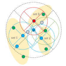
Figure 3: Adding nodes to $cds$ in Algorithm. 2

The algorithm ends once $\mathscr{S}$ contains only one subset that is not restricted (line 20). The algorithm returns $cds$ and the sum $\sum_{v\in ds}y\left(\left\{v\right\}\right)$ as $LB2$ (line 21).

Proposition 13.

Each node selected by Algorithm 2 is packed.

Proof.

Stems from the fact that the uniform increase of the $y\left(S\right)$ value is identical to Algorithm 1, and from Proposition 12. ∎

Algorithm 3

Receives a connected UDG graph $G=\left(V,E\right)$ with at least two nodes. The algorithm returns a data gathering tree $T=\left(V,E_{T}\right)$ in graph $G$, the selected MULE location $m$, and the approximation ratio $\alpha$ (from Theorem 7).

0:  A connected UDG $G=(V,E)$ with $\left|V\right|\geq 2$

0:  A gathering tree $T=\left(V,E_{T}\right)$, the selected location for the MULE $m$, and the MWCDS approximation ratio $\alpha$

1:  $E_{T}\leftarrow\emptyset$ , $cds\leftarrow\emptyset$

2:  for each $m^{\prime}\in V$ do

3:     $w\left(v\right)\leftarrow\left(2\cdot dist\left\{m^{\prime},v\right\}+C\right)\>\forall v\in V$

4:     $\left\{ds^{\prime}\,,\;LB1\right\}\leftarrow$ Algorithm 1 $\left(\,G\,,\;w\left(\cdot\right)\,\right)$

5:     $\left\{cds^{\prime}\,,\;LB2\right\}\leftarrow$ Algorithm 2 $\left(\,G\,,\;w\left(\cdot\right)\,,\;ds^{\prime}\,\right)$

6:     if $\sum_{v\in cds^{\prime}}w\left(v\right)<\sum_{v\in cds}w\left(v\right)$ then

7:        $m\leftarrow m^{\prime}$ , $LB\leftarrow LB1+LB2$ , $cds\leftarrow cds^{\prime}$

8:        $r\leftarrow$ The first node selected in $ds^{\prime}$ (at the first step of Algorithm 1)

9:     end if

10:  end for

11:  $SubG\leftarrow$ The induced subgraph of $cds$ in $G$

12:  $\bar{p}\leftarrow BFS\left(SubG\,,\;r\right)$ // Compute the predecessors of the nodes $v\in cds$ using BFS algorithm, starting from the root $r$

13:  for each $v\in cds\setminus\left\{r\right\}$ do

14:     $E_{T}\leftarrow E_{T}\cup\left\{DirectedEdge\left(v\rightarrow p_{v}\right)\right\}$ // $p_{v}$ is the predecessor of node $v$ (a component of $\bar{p}$)

15:  end for

16:  for each $u\in V\setminus\left(cds\cup\left\{r\right\}\right)$ do

17:     $v\leftarrow\underset{v\in cds}{\arg\min}\left\{dist\left\{u,v\right\}\right\}$

18:     $E_{T}\leftarrow E_{T}\cup\left\{DirectedEdge\left(u\rightarrow v\right)\right\}$

19:  end for

20:  return  $\left\{T=\left(V,E_{T}\right)\>,\quad m\>,\quad\alpha\leftarrow\nicefrac{{\sum_{v\in cds}w\left(v\right)}}{{LB}}\right\}$

Algorithm 3 Constructs a data gathering tree

The algorithm searches iteratively for the minimal weight CDS produced by Algorithm 2, over all possible MULE locations. The node weight function is determined to be $w\left(v\right)=\left(2\cdot dist\left\{m,v\right\}+C\right)$, according to Theorem 7. The algorithm uses Algorithm 1 to produce an IDS for Algorithm 2. The CDS with minimal weight is assigned to $cds$, the corresponding MULE location is assigned to $m$, $LB$ is the corresponding sum $LB1+LB2$, and $r$ is the first node selected for the corresponding $ds^{\prime}$.

After selecting the minimal weight CDS, the algorithm uses the BFS algorithm to construct a directed spanning tree towards the root node $r$, in the induced subgraph of $cds$ in $G$ (lines 11 - 15). In this way, the $cds$ nodes compose the BackBone of the gathering tree. Then, each node in $V\setminus cds$ is connected by an outgoing edge to the nearest node in $cds$.

Finally, the algorithm returns the result tree as $T$, the MULE location $m$, and the approximation ratio $\alpha$ of the result.

5.2 Correctness

In this section, we will show the correctness of our algorithms. We will emphasize in advance that the algorithms are required to receive a connected UDG graph with at least two nodes in order to return correct structures of IDS, CDS, and gathering tree. However, for the approximation ratio and for the lower bounds, additional constraints are required. For correct lower bounds ($LB1$ and $LB2$) and the $\alpha$ parameter, the graph should have a diameter of at least three. For correct approximation of the $\left(1,1\right)-MULE-UDG$ problem (i.e. $\left(1+\varepsilon\right)$), it is required to be hold $\underset{v\in V_{BB}^{\ast}}{Average}\left[dist\left\{m^{\ast},v\right\}\right]>1.3$, according to Theorem 7. As for graphs that do not meet only the first condition (on the diameter), these graphs are spread over a bounded area, and we will address this situation later in Subsection 5.3. We will show in a different approach that the result gathering tree still ensures the approximation required. As for graphs that do not meet the second condition, this issue still remains open.

Definition 14 (A feasible dual solution and lower bound).

Consider the MWCDS problem and the dual problem $MWCDS-D$. Vector $\bar{y}$ will be called a feasible dual solution, if $\bar{y}$ is proven to be a solution to the $MWCDS-D$ problem and satisfies all its constraints. A feasible lower bound is a value that has been proven to have a feasible dual solution which is well defined, whose sum $\sum_{S\subseteq V\vcentcolon S\neq\emptyset}f\left(S\right)\cdot y_{S}$ is equal to this value. $y_{S}$ are the components of $\bar{y}$, $V$ is the set of the graph nodes and $f\left(S\right)$ is defined in Equation 10.

Correctness of Algorithm 1.

Let $\text{$\mathscr{S}$}^{\prime}$ be the collection of all active subsets that Algorithm 1 maintains in the current step (i.e. $\text{$\mathscr{S}$}^{\prime}\subseteq\text{$\mathscr{S}$}$), and let $y^{\prime}\left(S\right)$ be the value the algorithm assigns to subset $S$ in the current step. We define the vector $\bar{y}^{\prime}$ of size $\left|\text{$\mathscr{S}$}\right|$ (where $y^{\prime}_{S}$ are its components) as follows:

$$y^{\prime}_{S}=\begin{cases}y^{\prime}\left(S\right)&for\;\left|S\right|=1\\ 0&for\;\left|S\right|>1\end{cases}\quad\forall S\in\text{$\mathscr{S}$}\,.$$ (14)

$\epsilon$ is the potential value of the selected node in the current step. $A$ is the set of nodes that the algorithm has selected up to the current step. From Lemma 19, Algorithm 1 returns an IDS. From Lemma 20, if the graph diameter is at least three then it returns a feasible lower bound.

Proposition 15.

Once node $v$ is selected by Algorithm 1 it becomes packed and $\epsilon\left(v\right)=\infty$, and it remains so until the end.

Proof.

From Proposition 12, after node $v$ is chosen by the algorithm it is packed. According to lines 7 and 9, after node $v$ is chosen, there is $\sum_{S\in\text{$\mathscr{S}$}^{\prime}\colon v\in N\left(S\right)}g\left(S\right)=0$, and therefore by Equation 13 $\epsilon\left(v\right)=\infty$. The only place that can change the packaging condition or the $\infty$ potential value is in line 14, since only here the algorithm performs $g\left(S^{\prime}\right)\leftarrow 1$. But this assignment is performed only for new subsets. For both conditions, subset $S^{\prime}$ will influence node $v$ only if $v\in N\left(S^{\prime}\right)$. New subsets are of the form $V\setminus\left\{u\right\}$, and they have only one neighbor which is $u$. Since node $v$ is already selected and added to $A$, it is not contained in the set $V\setminus A$. Hence, according to line 11, the subset $V\setminus\left\{v\right\}$ will not be added later in the algorithm. Therefore, new subsets will not influence node $v$, which will remain packed and $\epsilon\left(v\right)=\infty$. ∎

Proposition 16.

In Algorithm 1, if $g\left(S\right)=0$ for all $S\in\text{$\mathscr{S}$}^{\prime}$, then there must be $A=V$.

Proof.

Let us assume in contradiction that $g\left(S\right)=0\;\forall S\in\text{$\mathscr{S}$}^{\prime}$, but $A\neq V$. If so, there must be a node $u\in V\setminus A$, and from lines 12 - 14, there must be a subset $V\setminus\left\{u\right\}\in\text{$\mathscr{S}$}^{\prime}$ which is adjacent to $u$. Since $u$ is the only neighbor of $V\setminus\left\{u\right\}$, and $u$ is not yet selected by the algorithm, then the if statement in line 9 never met, nor does the assignment $g\left(V\setminus\left\{u\right\}\right)\leftarrow 0$. This is in contradiction to the assumption $g\left(S\right)=0\;\forall S\in\text{$\mathscr{S}$}^{\prime}$, and therefore must be $A=V$. ∎

Proposition 17.

The set $ds$ constructed by Algorithm 1 is an IS, and if $A=V$ then $ds$ must be a MIS.

Proof.

The set $ds$ is IS, since, in line 6 a node is added to $ds$ only if it is independent of the $ds$ nodes. Note that by line 5, if there is a step where $A=V$, it requires that each node was selected at least once. Let us assume in contradiction that $A=V$, but the set $ds$ is not a MIS. Then there is at least one node $v\in V\setminus ds$ that can be added to $ds$, so it must be $v\notin N\left(ds\right)\cup ds$. But since $v$ is already chosen by the algorithm, it is in contradiction to the condition in line 6. Hence, $ds$ must be MIS. ∎

Proposition 18.

Each node is selected at most once during Algorithm 1.

Proof.

According to Proposition 15, the potential value of each node $v\in V$ selected by the algorithm becomes $\epsilon\left(v\right)=\infty$, and remains so until the end. We want to show that there is no step in which a node is selected with a potential value of $\epsilon\left(v\right)=\infty$. To do this, let us assume in contradiction that there is a step where node $v$ is selected with $\epsilon\left(v\right)=\infty$, but the stop condition (line 17) has not yet met. Then, according to line 4, for each node $u\in V$ holds $\epsilon\left(u\right)=\infty$. Since $c_{u}<\infty$, then it must be the first case in Equation 13. The graph is connected with at least two nodes, so each subset in $\text{$\mathscr{S}$}^{\prime}$ is adjacent to at least one node. Therefore, must be $g\left(S\right)=0$ for all $S\in\text{$\mathscr{S}$}^{\prime}$, and according to Proposition 16, must also hold $A=V$. Consequently, from Proposition 17, the set $ds$ must be a MIS, hence it is also a DS. This is in contradiction to the assumption that $N\left(ds\right)\cup ds\neq V$. Therefore, the claim is correct and node can not be selected twice. ∎

Lemma 19.

Given a connected UDG with at least two nodes and node weights $w\left(\cdot\right)\colon V\rightarrow R^{+}$, Algorithm 1 returns an IDS.

Proof.

First, we argue that the set $ds$ contains at least one node. Since the graph is connected and has at least two nodes, and $\text{$\mathscr{S}$}^{\prime}$ is initialized to be $\left\{\left\{v\right\}\vcentcolon v\in V\right\}$, then at the first iteration, each node $v\in V$ has at least one subset $S\in\text{$\mathscr{S}$}^{\prime}$ for which $v\in N\left(S\right)$. Without loss of generality, let us consider node $v$ and some subset $S$, where $v\in N\left(S\right)$. From line 2, $g\left(S\right)\leftarrow 1$, so for node $v$ holds: $\sum_{S\in\text{$\mathscr{S}$}^{\prime}\colon v\in N\left(S\right)}g\left(S\right)>0$. Since also $c_{v}=\frac{1}{100}\cdot w\left(v\right)<\infty$, then from Equation 13, at least node $v$ will be selected at the first iteration, and $\epsilon$$\leq\epsilon\left(v\right)<\infty$.

From line 17, we can see that the algorithm halts once set $ds$ becomes a DS. In Proposition 18, we saw that each node can be selected at most once. Then the iterations must be halt, and this is as a result of the fact that the set $ds$ has become a DS.

Combine all that with Proposition 17, we get that $ds$ is both IS and DS. Therefore it is an IDS, and hence the lemma is correct. ∎

Lemma 20.

Given a connected UDG with a diameter of at least three and node weights $w\left(\cdot\right)\colon V\rightarrow R^{+}$, Algorithm 1 returns a feasible lower bound, having $\bar{y}^{\prime}$ as its feasible dual solution that also satisfies $\sum_{S\in\text{$\mathscr{S}$}\colon v\in N\left(S\right)}y^{\prime}_{S}\leq\frac{1}{100}\cdot w\left(v\right)\;\forall v\in V$.

Proof.

We will prove by induction on the algorithm steps that it maintains the constraints $\sum_{S\in\text{$\mathscr{S}$}^{\prime}\colon v\in N\left(S\right)}y^{\prime}\left(S\right)\leq c_{v}\;\forall v\in V$. Since at the initialization phase $y^{\prime}\left(S\right)=0\quad\forall S\in\text{$\mathscr{S}$}^{\prime}$ (line 2) and since $c_{v}>0$, then it is easy to see that the constraints are maintained for base case $step=0$. The induction hypothesis is that the statement is correct up to $step=k$, and we will prove that the statement remains correct for $step=k+1$. Note, the only line that can violate the constraints is line 8, where $y^{\prime}\left(S\right)$ is updated. In step $k+1$, the algorithm selects node $v$. Therefore, according to Proposition 12, node $v$ is packed, i.e. $\sum_{S\in\text{$\mathscr{S}$}^{\prime}\colon v\in N\left(S\right)}y^{\prime}\left(S\right)=c_{v}$, and according to Proposition 15, it remains packed until the end of the algorithm. Then, nodes where the statement can be violated are only those that have not yet been selected (i.e. from $V\setminus A$). Let us assume in contradiction that there is a node $u\in V\setminus A$ that after step $k+1$ violates the statement, and let $y^{\prime}_{k}\left(S\right)$ be the value of $y^{\prime}\left(S\right)$ at step $k$. We can write:

$$\begin{array}[]{rlc}\sum_{S\in\text{$\mathscr{S}$}^{\prime}\colon u\in N\left(S\right)}y^{\prime}\left(S\right)>&c_{u}\\ \sum_{S\in\text{$\mathscr{S}$}^{\prime}\colon u\in N\left(S\right)}\left(y^{\prime}_{k}\left(S\right)+g\left(S\right)\epsilon\left(v\right)\right)>&c_{u}\\ \epsilon\left(v\right)>&\frac{c_{u}-\sum_{S\in\text{$\mathscr{S}$}^{\prime}\colon u\in N\left(S\right)}y^{\prime}_{k}\left(S\right)}{\sum_{S\in\text{$\mathscr{S}$}^{\prime}\colon u\in N\left(S\right)}g\left(S\right)}=&\epsilon\left(u\right)\;.\end{array}$$

The result is in contradiction to the minimality of $\epsilon\left(v\right)$. So, the statement is correct for step $k+1$. Hence, the algorithm satisfies the constraints.

$\text{$\mathscr{S}$}^{\prime}$ contains subsets $\left\{v\right\}\vcentcolon v\in V$ (line 1) and $y^{\prime}_{S}=0\;\forall S:\left|S\right|>1$ (Equation 14), then we get $\sum_{S\in\text{$\mathscr{S}$}\colon v\in N\left(S\right)}y^{\prime}_{S}=\sum_{S\in\text{$\mathscr{S}$}^{\prime}\colon v\in N\left(S\right)}y^{\prime}_{S}$. Since $\sum_{S\in\text{$\mathscr{S}$}^{\prime}\colon v\in N\left(S\right)}y^{\prime}\left(S\right)\leq c_{v}$, then $\epsilon\left(v\right)\geq 0$ (Equation 13). Combine it with line 8, we get $y^{\prime}\left(S\right)\geq 0$. So, from Equation 14, $y^{\prime}_{S}\leq y^{\prime}\left(S\right)$. Recall that $c_{v}\triangleq\frac{1}{100}\cdot w\left(v\right)$. Then the following holds:

$$\sum_{S\in\text{$\mathscr{S}$}\colon v\in N\left(S\right)}y^{\prime}_{S}\leq\sum_{S\in\text{$\mathscr{S}$}^{\prime}\colon v\in N\left(S\right)}y^{\prime}\left(S\right)\leq c_{v}=\frac{1}{100}\cdot w\left(v\right)\leq w\left(v\right)\;\forall v\in V\,.$$

Since also $y^{\prime}_{S}\geq 0$ (Equation 14), then vector $\bar{y}^{\prime}$ satisfies all the constraints of $MWCDS-D$. Hence, $\bar{y}^{\prime}$ is a feasible dual solution.

Since the diameter of the graph is at least three, no subset of a single node is a DS. That is, $f\left(\left\{v\right\}\right)=1\;\forall v\in V$ (Equation 10). Combine it with Equation 14 and line 18, we get

$$\sum_{S\subseteq V\vcentcolon S\neq\emptyset}f\left(S\right)\cdot y^{\prime}_{S}=\sum_{S\subseteq V\vcentcolon S\neq\emptyset}y^{\prime}_{S}=\sum_{S\subseteq V\colon\left|S\right|=1}y^{\prime}\left(S\right)=\sum_{v\in V}y^{\prime}\left(\left\{v\right\}\right)=LB1\,.$$ (15)

Therefore, by Definition 14, $LB1$ is a feasible lower bound and $\bar{y}^{\prime}$ is its feasible dual solution. Hence, the lemma is correct. ∎

Correctness of Algorithm 2.

Let $\text{$\mathscr{S}$}^{\prime\prime}$ be the collection of the active subsets that Algorithm 2 maintains in the current step (i.e. $\text{$\mathscr{S}$}^{\prime\prime}\subseteq\text{$\mathscr{S}$}$), and let $y^{\prime\prime}\left(S\right)$ be the value that the algorithm assigns to subset $S$ in the current step. We define the vector $\bar{y}^{\prime\prime}$ of size $\left|\text{$\mathscr{S}$}\right|$ (where $y^{\prime\prime}_{S}$ are its components) as follows:

$$y^{\prime\prime}_{S}=\begin{cases}y^{\prime\prime}\left(S\right)&for\;S=\left\{v\right\}\vcentcolon v\in ds\\ 0&otherwise\end{cases}\quad\forall S\in\text{$\mathscr{S}$}\,.$$ (16)

$\epsilon$ is the potential value of the selected node in the current step. Let $\text{$\mathscr{S}$}^{1}$ be the collection of all un-restricted active subsets that contain some neighbor of the selected node, and $\text{$\mathscr{S}$}^{2}$ be the collection of all subsets in $\text{$\mathscr{S}$}^{1}$ that also contain a node which is both a neighbor of the selected node and belongs to the $cds$ set. From Lemma 27, Algorithm 2 returns a CDS. From Lemma 28, if the graph diameter is at least three and node weights are $w\left(v\right)=2\cdot dist\left\{m,v\right\}+C$, then it returns a feasible lower bound.

Proposition 21.

At each step of Algorithm 2, if node $v$ is contained in some active subset, then there must be an un-restricted subset which contains $v$.

Proof.

We will prove by induction on the steps, for each node separately. Without loss of generality, let $v$ be the node. The base case is the earliest step in which $v$ is contained in a subset. Let $k_{0}$ be this step and $S_{0}$ be this subset. If $v\in ds$, then by lines 1 and 2, the base case is trivial. If $v\notin ds$, then by line 18, $v$ must be selected by the algorithm to be contained in $S_{0}$. By line 19, the condition holds for the base case. If $v$ is never selected, then it is irrelevant. The induction hypothesis is that the statement holds for step $k>k_{0}$, and we will prove that the statement still holds for step $k+1$. According to the induction hypothesis, at step $k$ there is an un-restricted subset $S^{\prime}$ which contains $v$. Let $u$ be the node selected at step $k+1$. If $u\notin N\left(S^{\prime}\right)$, then by line 16, the situation remains the same. Let $S$ be the new subset at step $k+1$. If $u\in N\left(S^{\prime}\right)$, then $S^{\prime}\in\text{$\mathscr{S}$}^{1}$ (line 5) and therefore $v\in S$ (line 18). In line 19, $g\left(S\right)\leftarrow 1$, so the statement holds. Hence the claim is correct. ∎

Proposition 22.

After node $v$ is selected by Algorithm 2 it becomes packed and $\epsilon\left(v\right)=\infty$. Once a node becomes packed or the potential value becomes $\infty$, it remains so until the end.

Proof.

From Proposition 13, after node $v$ is selected by the algorithm it is packed. According to lines 14 and 16, after node $v$ is selected, there is $\sum_{S\in\text{$\mathscr{S}$}^{\prime\prime}\colon v\in N\left(S\right)}g\left(S\right)=0$, and therefore by Equation 13, $\epsilon\left(v\right)=\infty$. The only place that can change the packing condition or the $\infty$ potential value is in line 19, since only here the algorithm performs $g\left(S\right)\leftarrow 1$. But this assignment is performed only for new subsets. For both conditions, subset $S$ will influence node $v$ only if $v\in N\left(S\right)$ and the assignment $g\left(S\right)\leftarrow 1$ will be performed. Let us assume in contradiction that there is a new subset that influences $v$ at some later step. Let $k$ be the earliest step in which $v$ is influenced. Let $S$ be the new subset created in this step, and $u$ be the selected node. $S$ consists of all nodes of subsets $S^{\prime}\in\text{$\mathscr{S}$}^{\prime\prime}\vcentcolon g\left(S^{\prime}\right)=1,S^{\prime}\cap N\left(\left\{u\right\}\right)\neq\emptyset$ and node $u$. None of these subsets can be adjacent to $v$ at step $k-1$, since $\epsilon\left(v\right)=\infty$. Therefore, the only possibility to influence $v$ is if $u$ and $v$ are neighbors. From Proposition 21, there is a subset $S^{\prime\prime}\in\text{$\mathscr{S}$}^{\prime\prime}\vcentcolon v\in S^{\prime\prime},g\left(S^{\prime\prime}\right)=1$. By line 5, $S^{\prime\prime}\in\text{$\mathscr{S}$}^{1}$, and therefore $v\in S$. This is in contradiction to the assumption that $S$ influences $v$. Hence the claim is correct. ∎

Proposition 23.

Algorithm 2 does not select a node with potential value $\infty$.

Proof.

Let us assume in contradiction that there is a step in which the algorithm selects a node with potential value $\infty$. Consider $k$ to be the earliest step at which such a node is selected, and let $v$ be this node. By line 4, must hold $\epsilon\left(u\right)=\infty$ for all $u\in V$. From Equation 13, and since $c_{v}<\infty$, it requires that $\sum_{S\in\text{$\mathscr{S}$}^{\prime\prime}\colon u\in N\left(S\right)}g\left(S\right)=0$ for all $u\in V$. Since the graph is connected, it implies that there is no un-restricted subset $S\in\text{$\mathscr{S}$}^{\prime\prime}\vcentcolon\left|S\right|<\left|V\right|$. According to line 19, we know that there must be an un-restricted subset $S^{\prime}\in\text{$\mathscr{S}$}^{\prime\prime}$. Then this subset must be $S^{\prime}=V$. So it also has to be the only un-restricted subset. This is in contradiction to the stop condition (line 20) at the end of step $k-1$. Hence the claim is correct. ∎

Proposition 24.

At each step of Algorithm 2, the union of all un-restricted active subsets contains the set $cds$.

Proof.

By line 1, nodes from $ds$ are contained in some active subset $S$. As for nodes from $cds\setminus ds$, each node had to be selected by the algorithm to be added to $cds$. Thus, by line 18, this node was also added to some active subset. According to Proposition 21, a node that is contained in some active subset must also be contained in an un-restricted subset. Hence, all the nodes in $cds$ are included in the union. ∎

Proposition 25.

During Algorithm 2, no node from subset $ds$ will be selected.

Proof.

Let $v$ be some node from $ds$. Since $ds$ is an IS, at the initialization stage (line 1) there is no subset $S\in\text{$\mathscr{S}$}^{\prime\prime}$ adjacent to $v$. So, $\sum_{S\in\text{$\mathscr{S}$}^{\prime\prime}\colon v\in N\left(S\right)}g\left(S\right)=0$, and as a result $\epsilon\left(v\right)=\infty$. From propositions 22 and 23, the potential value of $v$ remains $\infty$ until the end, and therefore the node will not be selected by the algorithm. ∎

Proposition 26.

For each node $v\in S\vcentcolon S\in\text{$\mathscr{S}$}^{\prime\prime}$, if $v\notin cds$ then it must have a neighbor $u\in S\cap cds$.

Proof.

Consider some node $v$ and some subset $S$, where $S\in\text{$\mathscr{S}$}^{\prime\prime}$ and $v\in S\setminus cds$. Of course $v\notin ds$, consequently $v$ was not added to $S$ at the initialization stage (step $0$), but rather in a later step, say step $k>0$. Note that from propositions 13, 22 and 23, after node $v$ is selected, $\epsilon\left(v\right)=\infty$ until the end of the algorithm, and so it will not be selected again. Without loss of generality, let $S$ be the first subset $v$ added to. Otherwise, since $v$ will not be selected again, by line 18 all other subsets containing $v$ also contain all $S$ nodes. Since $ds$ is a DS and $v\notin ds$, then there is a node $u\in ds\cap N\left(\left\{v\right\}\right)$. Note that in step $0$, $u$ was contained in some subset, and therefore, according to Proposition 21, in step $k-1$, there is a subset $S^{\prime}\in\text{$\mathscr{S}$}^{\prime\prime}\vcentcolon u\in S^{\prime},g\left(S^{\prime}\right)=1$. In step $k$, $S^{\prime}$ will be included in the collection $\text{$\mathscr{S}$}^{1}$. We assumed that $v\notin cds$, so it must be because the condition in line 7 is not met. Thus it requires that $\left|\text{$\mathscr{S}$}^{1}\right|=1$, and only $S^{\prime}$ contained in $\text{$\mathscr{S}$}^{1}$. Recall that the neighbor $u\in S^{\prime}\cap ds$, hence $u\in S^{\prime}\cap cds$. According to line 18, $S$ contains $v$ and all $S^{\prime}$ nodes, and therefore the claim is correct. ∎

Lemma 27.

Given a connected UDG with at least two nodes, node weights $w\left(\cdot\right)\colon V\rightarrow R^{+}$, and an IDS, Algorithm 2 returns a CDS.

Proof.

First, we will show that the algorithm halts. From Proposition 13, the selected node is packed, and according to Proposition 22, it remains so until the end. Thus after a node is selected, its potential value will remain $\infty$. According to Proposition 23, this node will not be selected again. Hence, the algorithm must halts after at most $\left|V\right|$ steps.

We will show that the resulting $cds$ is indeed CDS. Since $cds$ contains $ds$ then it is dominates all $V$ nodes.

After the algorithm halts, by line 20, there must be $\sum_{S\in\text{$\mathscr{S}$}^{\prime\prime}}g\left(S\right)=1$. According to Proposition 24, the only un-restricted subset $S\in\text{$\mathscr{S}$}^{\prime\prime}$ must contain $cds$. We will prove by induction on the algorithm steps that it maintains the intersection $S^{\prime}\cap cds$ connected for each $S^{\prime}\in\text{$\mathscr{S}$}^{\prime\prime}$ (and especially for $S$).
According to line 1, initially, each subset $S^{\prime}\in\text{$\mathscr{S}$}^{\prime\prime}$ contains a single node from $ds$. So the base case is trivial. The induction hypothesis is that the statement holds for step $k$, and we will prove that the statement still holds for step $k+1$. The only new subset added during step $k+1$ is in line 19. Consider $S^{\prime}$ to be the new subset and $v$ to be the selected node. $ds$ is a DS, and by Proposition 25, we know that $v$ is not in $ds$. Then, there is a node $u\in ds$ which is $u\in N\left(\left\{v\right\}\right)$. By line 1, $u$ is contained in some subset, so according to Proposition 21, there is a subset $S^{\prime\prime}\vcentcolon u\in S^{\prime\prime}$ that satisfies $g\left(S^{\prime\prime}\right)=1$. Therefore, $\text{$\mathscr{S}$}^{1}$ contains at least the subset $S^{\prime\prime}$.
If the condition in line 7 is not met, then $v$ is not added to $cds$, and $\text{$\mathscr{S}$}^{1}$ contains only $S^{\prime\prime}$. From the induction hypothesis the statement holds, since $S^{\prime}\cap cds=\left(S^{\prime\prime}\cup\left\{v\right\}\right)\cap cds=S^{\prime\prime}\cap cds$.
If the condition in line 7 is met, then $v$ is added to $cds$ and $\left|\text{$\mathscr{S}$}^{1}\right|>1$. We will show that $\left(S^{\prime\prime}\cup\left\{v\right\}\right)\cap cds$ is CS, for all $S^{\prime\prime}\in\text{$\mathscr{S}$}^{1}$. Therefore, by line 18, $S^{\prime}\cap cds$ must also be connected. Note that $\text{$\mathscr{S}$}^{2}\subseteq\text{$\mathscr{S}$}^{1}$. If $S^{\prime\prime}\in\text{$\mathscr{S}$}^{2}$, then $v$ has a neighbor $u\in S^{\prime\prime}\cap cds$. Hence $\left(S^{\prime\prime}\cup\left\{v\right\}\right)\cap cds$ is also CS. If $S^{\prime\prime}\in\text{$\mathscr{S}$}^{1}\setminus\text{$\mathscr{S}$}^{2}$, then by lines 9 - 12, the algorithm adds to $cds$ some neighbor of $v$. Let $u$ be this neighbor, and note that $u\notin cds$. From Proposition 26, $u$ has a neighbor in $S^{\prime\prime}\cap cds$, then $S^{\prime\prime}\cap\left(cds\cup\left\{u\right\}\right)$ is CS. After line 11, $S^{\prime\prime}\cap cds$ remains connected, and so is $\left(S^{\prime\prime}\cup\left\{v\right\}\right)\cap cds$.
The statement holds for step $k+1$. Therefore, $S^{\prime}\cap cds$ is a CS for each $S^{\prime}\in\text{$\mathscr{S}$}^{\prime\prime}$.

If we consider the last step, $S\cap cds$ is also a CS. Since $S\cap cds=cds$, then $cds$ must also be a CDS. Therefore, the lemma is correct. ∎

Lemma 28.

Given a connected UDG with a diameter of at least three and node weights $w\left(v\right)=2\cdot dist\left\{m,v\right\}+C$, Algorithm 2 returns a feasible lower bound, having $\bar{y}^{\prime\prime}$ as its feasible dual solution that also satisfies $\sum_{S\in\text{$\mathscr{S}$}\colon v\in N\left(S\right)}y^{\prime\prime}_{S}\leq\frac{99}{100}\cdot w\left(v\right)\;\forall v\in V$.

Proof.

We will prove by induction on the algorithm steps that it maintains the constraints $\sum_{S\in\text{$\mathscr{S}$}^{\prime\prime}\colon v\in N\left(S\right)}y^{\prime\prime}\left(S\right)\leq c_{v}\;\forall v\in V$. In the initialization phase $\text{$\mathscr{S}$}^{\prime\prime}\triangleq\left\{\left\{v\right\}\vcentcolon v\in ds\right\}$, so $\sum_{S\in\text{$\mathscr{S}$}^{\prime\prime}\colon v\in N\left(S\right)}y^{\prime\prime}\left(S\right)=\sum_{u\in ds\colon v\in N\left(\left\{u\right\}\right)}y^{\prime\prime}\left(\left\{u\right\}\right)$. Recall that $y^{\prime\prime}\left(\left\{u\right\}\right)$ are initialized to $\frac{99}{500}\cdot\left(w\left(u\right)-2\right)$. Since node weights are $w\left(u\right)\triangleq 2\cdot dist\left\{m,u\right\}+C$ and the distance between a pair of neighbors in UDG is at most $1$, then $w\left(u\right)\leq w\left(v\right)+2\vcentcolon v\in N\left(\left\{u\right\}\right)$. $ds$ is an IS in UDG. Therefore, each node in the graph can have at most $5$ neighbors in $ds$ (the kissing number problem). Formally, $\left|ds\cap N\left(\left\{v\right\}\right)\right|\leq 5\;\forall v\in V$. When we put it all together:

$$\begin{array}[]{rl}{\displaystyle\sum_{S\in\text{$\mathscr{S}$}^{\prime\prime}\colon v\in N\left(S\right)}}y^{\prime\prime}\left(S\right)=&{\displaystyle\sum_{u\in ds\colon v\in N\left(\left\{u\right\}\right)}}y^{\prime\prime}\left(\left\{u\right\}\right)\\ =&{\displaystyle\sum_{u\in ds\colon v\in N\left(\left\{u\right\}\right)}}\frac{99}{500}\cdot\left(w\left(u\right)-2\right)\\ \leq&{\displaystyle\sum_{u\in ds\colon v\in N\left(\left\{u\right\}\right)}}\frac{99}{500}\cdot\left(\left(w\left(v\right)+2\right)-2\right)\\ =&\left|ds\cap N\left(\left\{v\right\}\right)\right|\cdot\frac{99}{500}\cdot w\left(v\right)\\ \leq&5\cdot\frac{99}{500}\cdot w\left(v\right)=\frac{99}{100}\cdot w\left(v\right)=c_{v}\;.\end{array}$$

Thus the statement is correct for base case $step=0$. The induction hypothesis is that the statement is correct up to $step=k$, and we will prove that the statement remains correct for $step=k+1$. Note, the only line that can violate the constraints is line 15, where $y^{\prime\prime}\left(S\right)$ is updated. In step $k+1$, the algorithm selects node $v$. Therefore, according to Proposition 13, node $v$ is packed, i.e. $\sum_{S\in\text{$\mathscr{S}$}^{\prime\prime}\colon v\in N\left(S\right)}y^{\prime\prime}\left(S\right)=c_{v}$, and according to Proposition 22, it remains packed until the end of the algorithm. Then, nodes where the statement can be violated are only those that have not yet been selected. Let us assume in contradiction that there is a node $u$ that has not yet been packed and after step $k+1$ violates the statement. Let $y^{\prime\prime}_{k}\left(S\right)$ be the value of $y^{\prime\prime}\left(S\right)$ at step $k$. So, we can write:

$$\begin{array}[]{rlc}\sum_{S\in\text{$\mathscr{S}$}^{\prime\prime}\colon u\in N\left(S\right)}y^{\prime\prime}\left(S\right)>&c_{u}\\ \sum_{S\in\text{$\mathscr{S}$}^{\prime\prime}\colon u\in N\left(S\right)}\left(y^{\prime\prime}_{k}\left(S\right)+g\left(S\right)\epsilon\left(v\right)\right)>&c_{u}\\ \epsilon\left(v\right)>&\frac{c_{u}-\sum_{S\in\text{$\mathscr{S}$}^{\prime\prime}\colon u\in N\left(S\right)}y^{\prime\prime}_{k}\left(S\right)}{\sum_{S\in\text{$\mathscr{S}$}^{\prime\prime}\colon u\in N\left(S\right)}g\left(S\right)}=&\epsilon\left(u\right)\;.\end{array}$$

In contradiction to the minimality of $\epsilon\left(v\right)$. Thus the statement is correct for step $k+1$. Hence, the algorithm satisfies the constraints.

$\text{$\mathscr{S}$}^{\prime\prime}$ contains subsets $\left\{v\right\}\vcentcolon v\in ds$ (line 1) and $y^{\prime\prime}_{S}=0\;\forall S\notin\left\{\left\{v\right\}\vcentcolon v\in ds\right\}$ (Equation 16), then we get $\sum_{S\in\text{$\mathscr{S}$}\colon v\in N\left(S\right)}y^{\prime\prime}_{S}=\sum_{S\in\text{$\mathscr{S}$}^{\prime\prime}\colon v\in N\left(S\right)}y^{\prime\prime}_{S}$. Since $\sum_{S\in\text{$\mathscr{S}$}^{\prime\prime}\colon v\in N\left(S\right)}y^{\prime\prime}\left(S\right)\leq c_{v}$, then $\epsilon\left(v\right)\geq 0$ (Equation 13). By combining this with line 15, we get $y^{\prime\prime}\left(S\right)\geq 0$. Consequently, from Equation 16, $y^{\prime\prime}_{S}\leq y^{\prime\prime}\left(S\right)$. Recall that $c_{v}\triangleq\frac{99}{100}\cdot w\left(v\right)$. Then the following holds:

$$\sum_{S\in\text{$\mathscr{S}$}\colon v\in N\left(S\right)}y^{\prime\prime}_{S}\leq\sum_{S\in\text{$\mathscr{S}$}^{\prime\prime}\colon v\in N\left(S\right)}y^{\prime\prime}\left(S\right)\leq c_{v}=\frac{99}{100}\cdot w\left(v\right)\leq w\left(v\right)\;\forall v\in V\,.$$

Since also $y^{\prime\prime}_{S}\geq 0$ (Equation 16), then vector $\bar{y}^{\prime\prime}$ satisfies all the constraints of $MWCDS-D$. Hence, $\bar{y}^{\prime\prime}$ is a feasible dual solution.

Since the diameter of the graph is at least three, so no subset of a single node is a DS. That is, $f\left(\left\{v\right\}\right)=1\;\forall v\in ds$ (Equation 10). Combine it with Equation 16 and line 21, we get

$$\sum_{S\subseteq V\vcentcolon S\neq\emptyset}f\left(S\right)\cdot y^{\prime\prime}_{S}=\sum_{S\in\text{$\mathscr{S}$}}y^{\prime\prime}_{S}=\sum_{v\in ds}y^{\prime\prime}\left(\left\{v\right\}\right)=LB2\,.$$ (17)

Therefore, by Definition 14, $LB2$ is a feasible lower bound and $\bar{y}^{\prime\prime}$ is its feasible dual solution. Hence, the lemma is correct. ∎

Correctness of Algorithm 3.

From Lemma 29, Algorithm 3 returns a data gathering tree and its corresponding MULE location. From Lemma 30, if the graph diameter is at least three then it returns a feasible approximation ratio.

Lemma 29.

Given a connected UDG with at least two nodes, Algorithm 3 returns a data gathering tree and its corresponding MULE location.

Proof.

According to lines 14 and 18, the structure consists of directed edges.
Since the node weight function is $0<w\left(\cdot\right)<\infty$ (line 3) and $\left|V\right|\geq 2$, then according to Lemma 19 the subset $ds^{\prime}$ that produces Algorithm 1 (line 4) is an IDS, and according to Lemma 27, the subset $cds^{\prime}$ produced by Algorithm 2 (line 5) is a CDS. From line 7, also $cds$ is a CDS. Let $SubG$ be the induced sub graph of $cds$ in $G$. So, since $G$ is a connected graph and $cds$ is a CS, then $SubG$ is a connected graph. By line 8, $r\in ds^{\prime}$, therefore, $r$ is a node in $SubG$. In line 12, since the BFS algorithm starts at node $r$ and the graph is connected, then at line 14 at least one incoming edge must be added to $r$. From lines 13, 14, 16 and 18, we see that each node (except $r$) has a directed outgoing edge in the structure. Hence, we can say that the structure spans all the nodes in $G$.
From the BFS mechanism to finding shortest paths, and since for each node in $cds\setminus\left\{r\right\}$, an added edge is directed to its predecessor, after the for loop of line 13, $r$ is reachable from all $cds\setminus\left\{r\right\}$ nodes in the sub graph $SubG$. After the for loop of line 16, it can be reached from any of the other nodes of $V$ to some node in $cds$. Therefore, $r$ is also reachable from all the nodes in the structure.
Since $G$ is a connected UDG and $cds$ is a DS, note that each directed edge in the structure is added only between a pair of neighbors, so it is also an undirected edge in $G$.
We have seen that the structure that constructs Algorithm 3 is a directed spanning tree in $G$, and that $r$ is reachable from all nodes. Thus, by Definition 1, it can be said that the structure is a data gathering tree and $r$ is its root.

According to the last iteration where line 7 is performed, we can see that $m$ is the MULE location used for building $cds$, which is used later on to build the gathering tree. Hence, the lemma is correct. ∎

Lemma 30.

Given a connected UDG with a diameter of at least three, Algorithm 3 returns a feasible approximation ratio $\alpha$.

Proof.

Consider $\bar{y}^{\prime}$ and $\bar{y}^{\prime\prime}$, to be the vector solution that constructs Algorithm 1 (Equation 14) and Algorithm 2 (Equation 16), respectively. According to lemmas 20 and 28, since node weights are $w\left(v\right)\triangleq 2\cdot dist\left\{m,v\right\}+C$ and the graph diameter is at least three, then holds $\sum_{S\in\text{$\mathscr{S}$}\colon v\in N\left(S\right)}y^{\prime}_{S}\leq\frac{1}{100}\cdot w\left(v\right)$ and $\sum_{S\in\text{$\mathscr{S}$}\colon v\in N\left(S\right)}y^{\prime\prime}_{S}\leq\frac{99}{100}\cdot w\left(v\right)$ for all $v\in V$. Consider vector $\bar{y}$ (where $y_{S}$ are its components) which is defined as follows: $\bar{y}\triangleq\bar{y}^{\prime}+\bar{y}^{\prime\prime}$. So we can write:

$$\begin{array}[]{rl}{\displaystyle\sum_{S\in\text{$\mathscr{S}$}\colon v\in N\left(S\right)}}y_{S}=&{\displaystyle\sum_{S\in\text{$\mathscr{S}$}\colon v\in N\left(S\right)}}\left(\bar{y}^{\prime}_{S}+\bar{y}^{\prime\prime}_{S}\right)\\ \leq&\frac{1}{100}\cdot w\left(v\right)+\frac{99}{100}\cdot w\left(v\right)\\ =&w\left(v\right)\;\forall v\in V\,.\end{array}$$

Since also $y_{S}=\bar{y}^{\prime}_{S}+\bar{y}^{\prime\prime}_{S}\geq 0$, then vector $\bar{y}$ satisfies all the constraints of $MWCDS-D$. Hence, $\bar{y}$ is a feasible dual solution. Using equations 15 and 17, we can also write:

$$\sum_{S\subseteq V\vcentcolon S\neq\emptyset}f\left(S\right)\cdot y_{S}=\sum_{S\subseteq V\vcentcolon S\neq\emptyset}f\left(S\right)\cdot y^{\prime}_{S}+\sum_{S\subseteq V\vcentcolon S\neq\emptyset}f\left(S\right)\cdot y^{\prime\prime}_{S}=LB1+LB2\,.$$

Therefore, by Definition 14, $LB=LB1+LB2$ is a feasible lower bound.

In Lemma 29, we showed that $cds$ is a CDS. Then by line 20 and from Definition 11, we can say that the value $\alpha$ returned by algorithm 3 is a feasible approximation ratio. ∎

5.3 Performance guarantees

In this section we show performance guarantees of Algorithm 3 (including algorithms 1 and 2) in the context of approximation and runtime. We analyze the approximation ratio of the gathering tree produced by Algorithm 3 with respect to the optimal gathering tree for the $\left(1,1\right)-MULE-UDG$ problem. According to Theorem 7, we show that if the input graph satisfies the condition $\underset{v\in V_{BB}^{\ast}}{Average}\left[dist\left\{m^{\ast},v\right\}\right]>1.3$, then the algorithm achieves an approximation of $20+\varepsilon$. It should be noted that for graphs that do not meet this condition, the problem still remains open. From now on, let us consider only graphs that satisfy the condition. Lemma 32 and Lemma 33 prove the approximation ratio. Further, we analyze the algorithm runtime and present optimizations that can achieve time complexity of $O\left(n^{3}\cdot\varDelta\left(G\right)\right)$, where $\varDelta\left(G\right)$ is the maximum degree in the graph and $n$ is the number of nodes.

Algorithm 3 produces a $\boldsymbol{\left(20+\varepsilon\right)-approximate}$ solution.

Let us refer to nodes in $cds\setminus ds$ as the ”connectors”, since they connect the $ds$ nodes.

Lemma 31.

There is an injective mapping function from each connector to a single node in $ds$, such that no more than two connectors are mapped to one node. The connector is at most one unit away from the node, and if there is an additional connector, then it is at most two units away.

Proof.

In order to prove this claim, we first build a spanning tree $T^{\prime}=\left(cds,E^{\prime}\right)$, which spans all $cds$ nodes. Then, based on $T^{\prime}$, we explain the mapping of each connector.

The construction of $T^{\prime}$ is based on the decisions made by Algorithm 2. For each node $v$ selected at each step, we add two types of edges. The first type is for each subset $S\in\text{$\mathscr{S}$}^{2}$, we add the edge $\left(v,u\right)$ to $E^{\prime}$, where $u\in S\cap N\left(\left\{v\right\}\right)\cap ds$ if there is one, and if not, $u\in S\cap N\left(\left\{v\right\}\right)\cap cds$. The second type of edges is for each subset $S\in\text{$\mathscr{S}$}^{1}\setminus\text{$\mathscr{S}$}^{2}$, we add the edge $\left(v,u\right)$ to $E^{\prime}$, where $u$ is a neighbor according to the choice of the algorithm in line 10. At the end, we go over all edges in $E^{\prime}$ and delete edges with nodes in $V\setminus cds$.

The proof that $T^{\prime}=\left(cds,E^{\prime}\right)$ is a spanning tree for $cds$ is done by induction on the algorithm steps. Recall that $\text{$\mathscr{S}$}^{\prime\prime}$ is the collection of all active subsets of Algorithm 2. We want to show that at each step and for each un-restricted active subset $S\in\text{$\mathscr{S}$}^{\prime\prime}$, the induced subgraph of $S\cap cds$ in $T^{\prime}$ is a spanning tree for the nodes in $S\cap cds$. The base case, step $0$, is trivial. The induction hypothesis is that the statement holds for step $k>0$, and we will prove that the statement still holds for step $k+1$. Consider $S^{\prime}$ to be the new subset created in step $k+1$. $S^{\prime}$ contains all subsets of $\text{$\mathscr{S}$}^{1}$. From the induction hypothesis for step $k$ and since each $S^{\prime\prime}\in\text{$\mathscr{S}$}^{1}$ is un-restricted, the induced subgraph of $S^{\prime\prime}\cap cds$ in $T^{\prime}$ is a spanning tree for $S^{\prime\prime}\cap cds$. Let $v$ be the selected node. Since $ds$ is a DS, then $v$ has a neighbor in $ds$. At initialization, this neighbor is contained in some subset. So, according to Proposition 21, implies that $\left|\text{$\mathscr{S}$}^{1}\right|>0$. If at the end of the algorithm $v\in cds$, then for each $S^{\prime\prime}\in\text{$\mathscr{S}$}^{1}$ one edge is added to $E^{\prime}$, and connects $S^{\prime\prime}\cap cds$ (also its sub spanning tree) to $v$. If eventually $v\notin cds$, then $v\notin S^{\prime\prime}\cap cds$ and its edges are deleted at the end. Since all edges are added in a star form around $v$, then the result structure is still a tree, and it also spans node $v$. Hence, it is a spanning tree for $S^{\prime}\cap cds$. According to the induction principle, the statement is correct for every step. In particular for the last step, in which $\text{$\mathscr{S}$}^{\prime\prime}$ contains only one un-restricted subset $S$. From Proposition 24 we know that $cds\subseteq S$, so $T^{\prime}$ is a spanning tree for $cds$.

The mapping function between the connectors and the $ds$ nodes is described as follows. Since the algorithm adds to $cds$, only connectors with at least two edges in $E^{\prime}$, then the connectors can not be leaves in $T^{\prime}$. Consider the root node $r$, we know that $r\in ds$. We go over all edges of $T^{\prime}$, and each edge we directed towards $r$. Each connector is mapped to the nearest (by hops) node in $ds$ which has a directed path to that connector. In case of multiple choice, select one arbitrarily.

The proof that we do not map to one node in $ds$, more than two connectors that meet the distance requirements is as follows. We will show that each connector $v\in cds\setminus ds$ has a node $u\in ds$ so that there is a directed path from $u$ to $v$ of a length no more than two hops. If $v$ has an incoming edge from a node in $ds$, then we are done. Otherwise, let us consider $v^{\prime}$ to be one of the connectors of the incoming edges (note, since $v$ is not a leaf then there must be one). Since $T^{\prime}$ is a directed tree towards a particular node, then $v^{\prime}$ has only one outgoing edge, and this edge is to $v$. All other edges of $v^{\prime}$ must be incoming. We have already seen that $\left|\text{$\mathscr{S}$}^{1}\right|>0$ since each selected node has a neighbor from $ds$ in $G$, so each connector has a neighbor from $ds$, also in tree $T^{\prime}$. Then, one of the incoming edges of $v^{\prime}$ must be from a node in $ds$, and let us denote this node by $u$. Thus, we have the path $u\rightarrow v^{\prime}\rightarrow v$ in $T^{\prime}$, and we are done.
Since $T^{\prime}$ is a directed tree towards a particular node, each node has only one outgoing edge. Therefore, each node from $ds$ can reach at most two connectors at a distance of two hops in $T^{\prime}$. These are the only two connectors that can be mapped to this node. Since we are dealing with an UDG, the first must be at most one unit away, and the second at most two units. Hence, we complete the proof. ∎

Lemma 32.

Given a connected UDG with a diameter of at least three, Algorithm 3 returns a $\left(20+\varepsilon\right)-approximate$ solution to the $\left(1,1\right)-MULE-UDG$ problem.

Proof.

Recall that $w\left(v\right)=2\cdot dist\left\{m,v\right\}+C$. According to Lemma 31, each node $v$ from $ds$ has at most two connectors in $cds\setminus ds$, where one connector has a weight greater by $2$ and the other by $4$, than $v$’s weight. Therefore, we can bound $cds$ weight by $Weight\left(cds\right)\leq\sum_{v\in ds}\left(3\cdot w\left(v\right)+6\right)$. In Algorithm 2 line 2, we assign initial $y$’s values, then we can bound $F_{\bar{y}}$ from below by $F_{\bar{y}}\geq\sum_{v\in ds}\frac{99}{500}\cdot\left(w\left(v\right)-2\right)$. Since both sums contain only the $ds$ nodes, we can calculate the ratio even for just a single node. Note that $w\left(v\right)\geq C$, and since $0<R_{M}<0.3$, then $C>14.5$ (Figure 2). So from Definition 11, we can state that the approximation ratio $\alpha$ is:

$$\frac{Weight\left(cds\right)}{F_{\bar{y}}} \leq\frac{\sum_{v\in ds}\left(3\cdot w\left(v\right)+6\right)}{\sum_{v\in ds}\frac{99}{500}\cdot\left(w\left(v\right)-2\right)}=\frac{3\cdot w\left(v\right)+6}{\nicefrac{{99}}{{500}}\cdot\left(w\left(v\right)-2\right)}=$$

$$=\frac{3}{\nicefrac{{99}}{{500}}}+\frac{6+6}{\nicefrac{{99}}{{500}}\cdot\left(w\left(v\right)-2\right)}\leq\frac{500}{99}\left(3+\frac{12}{\left(14.5-2\right)}\right)=20\;.$$ (18)

From Equation 12, $OPT_{cds^{\ast}}\geq F_{\bar{y}}$, then we can write:

$$\frac{Weight\left(cds\right)}{OPT_{cds^{\ast}}}\stackrel{{\scriptstyle\left(\ref{eq:T-R-P-12}\right)}}{{\leq}}\frac{Weight\left(cds\right)}{F_{\bar{y}}}\stackrel{{\scriptstyle\left(\ref{eq:P-G-1}\right)}}{{\leq}}20\;.$$ (19)

Let $T$ be the gathering tree that produces Algorithm 3 and $m$ is its MULE location. From Lemma 5 and since the tree’s BackBone is $cds$, we get:

$$Cost\left(T,m\right)\stackrel{{\scriptstyle\left(\ref{eq:R-T-M-1}\right)}}{{\leq}}\sum_{v\in V_{BB}}\left(2\cdot dist\left\{m,v\right\}+C\right)=\sum_{v\in cds}\left(2\cdot dist\left\{m,v\right\}+C\right)=Weight\left(cds\right)\;.$$ (20)

Let us distinguish between the two MULE locations, $m$ is the one chosen by the algorithm and $m^{\ast}$ of the optimal solution. Let $cds_{m}^{\ast}$ be the optimal solution of MWCDS for location $m$, where $cds_{m}$ is the CDS constructed by the algorithm, and $cds_{m^{\ast}}^{\ast}$ is for location $m^{\ast}$. The algorithm selects the minimal-weight CDS, so we have the following inequality:

$$20\cdot OPT_{cds_{m^{\ast}}^{\ast}}\stackrel{{\scriptstyle\left(\ref{eq:P-G-2}\right)}}{{\geq}}Weight\left(cds_{m^{\ast}}\right)\geq Weight\left(cds_{m}\right)\;.$$ (21)

Let $T^{\ast}$ be the optimal gathering tree and $m^{\ast}$ is its MULE location. From Theorem 7, $OPT_{T^{\ast}}>\left(1+\varepsilon\right)^{-1}\cdot OPT_{cds_{m^{\ast}}^{\ast}}$. So we can put it all together into one equation and conclude that:

$$\frac{Cost\left(T,m\right)}{OPT_{T^{\ast}}} \stackrel{{\scriptstyle\left(\ref{eq:R-T-M-2}\right)}}{{<}}\frac{Cost\left(T,m\right)}{\left(1+\varepsilon\right)^{-1}\cdot OPT_{cds_{m^{\ast}}^{\ast}}}\stackrel{{\scriptstyle\left(\ref{eq:P-G-3}\right)}}{{\leq}}\left(1+\varepsilon\right)\cdot\frac{Weight\left(cds_{m}\right)}{OPT_{cds_{m^{\ast}}^{\ast}}}\stackrel{{\scriptstyle\left(\ref{eq:P-G-4}\right)}}{{\leq}}$$

$$\stackrel{{\scriptstyle\left(\ref{eq:P-G-4}\right)}}{{\leq}}\left(1+\varepsilon\right)\cdot\frac{Weight\left(cds_{m}\right)}{20^{-1}\cdot Weight\left(cds_{m}\right)}=20\cdot\left(1+\varepsilon\right)=20+\varepsilon\;,$$

where the last equality is if we include the multiplication by $20$ into the inaccuracy $\varepsilon$. So that $\varepsilon\triangleq 20\left(\frac{2}{\left(C+2.6\right)}\cdot\left(\underset{v\in V_{BB}^{\ast}}{Average}\left[dist\left\{m^{\ast},v\right\}\right]-1.3\right)\right)^{-1}$. ∎

Lemma 33.

Given a connected UDG with a diameter of less than three, Algorithm 3 returns a $\left(20+\varepsilon\right)-approximate$ gathering tree to the $\left(1,1\right)-MULE-UDG$ problem.

Proof.

Since the graph is an UDG with a bounded area, then for each node $v\in V$ holds $dist\left\{m,v\right\}\leq 2$. Recall that the node weight function is $2\cdot dist\left\{m,v\right\}+C$, so we have $Weight\left(cds\right)\leq\left(4+C\right)\cdot\left|cds\right|$. From Lemma 31, we know that $\left|cds\right|\leq 3\cdot\left|ds\right|$. Therefore, we can write the following equation:

$$Weight\left(cds\right)\leq 3\cdot\left(4+C\right)\cdot\left|ds\right|\;.$$ (22)

Note that $w\left(v\right)\geq C$. Let $mcds^{\ast}$ be the optimal solution for the MCDS problem. Thus, since $cds^{\ast}$ is a CDS, it must be hold that $\left|cds^{\ast}\right|\geq\left|mcds^{\ast}\right|$. We obtain the following inequality:

$$OPT_{cds^{\ast}}=\sum_{v\in cds^{\ast}}w\left(v\right)\geq C\cdot\left|cds^{\ast}\right|\geq C\cdot\left|mcds^{\ast}\right|\;.$$ (23)

Let $mis$ be a maximal independent set. Weili Wu et al. [13] showed that for UDG graph, $\left|mis\right|\leq 3.8\cdot\left|mcds^{\ast}\right|+1.2$. From Proposition 17, $ds$ is a MIS, then

$$\left|ds\right|\leq 3.8\cdot\left|mcds^{\ast}\right|+1.2\;.$$ (24)

If we sum it all up here, we get:

$$\frac{Weight\left(cds\right)}{OPT_{cds^{\ast}}} \stackrel{{\scriptstyle\left(\ref{eq:P-G-5}\right)}}{{\leq}}\frac{3\cdot\left(4+C\right)\cdot\left|ds\right|}{OPT_{cds^{\ast}}}\stackrel{{\scriptstyle\left(\ref{eq:P-G-6}\right)}}{{\leq}}\frac{3\cdot\left(4+C\right)\cdot\left|ds\right|}{C\cdot\left|mcds^{\ast}\right|}\stackrel{{\scriptstyle\left(\ref{eq:P-G-7}\right)}}{{\leq}}$$

$$\stackrel{{\scriptstyle\left(\ref{eq:P-G-7}\right)}}{{\leq}}\frac{3\cdot\left(4+C\right)\cdot\left(3.8\cdot\left|mcds^{\ast}\right|+1.2\right)}{C\cdot\left|mcds^{\ast}\right|}=$$

$$=\frac{45.6\cdot\left|mcds^{\ast}\right|+11.4\cdot C\cdot\left|mcds^{\ast}\right|+14.4+3.6\cdot C}{C\cdot\left|mcds^{\ast}\right|}\;.$$

Recall that $C>14.5$, and $mcds^{\ast}$ is a DS, so it must contain at least one node, i.e. $\left|mcds^{\ast}\right|\geq 1$. We can continue the inequality as follows:

$$\frac{Weight\left(cds\right)}{OPT_{cds^{\ast}}}<\frac{45.6}{14.5}+11.4+\frac{14.4}{14.5\cdot 1}+\frac{3.6}{1}<19.14<20\;.$$ (25)

As in Lemma 32, let us distinguish between two MULE locations, $m$ and $m^{\ast}$. Remember that the algorithm selects the minimal-weight CDS, then we can state that:

$$20\cdot OPT_{cds_{m^{\ast}}^{\ast}}\stackrel{{\scriptstyle\left(\ref{eq:P-G-8}\right)}}{{>}}Weight\left(cds_{m^{\ast}}\right)\geq Weight\left(cds_{m}\right)\;.$$ (26)

Similarly to Lemma 32, we can put it all together and conclude that:

$$\frac{Cost\left(T,m\right)}{OPT_{T^{\ast}}} \stackrel{{\scriptstyle\left(\ref{eq:R-T-M-2}\right)}}{{<}}\frac{Cost\left(T,m\right)}{\left(1+\varepsilon\right)^{-1}\cdot OPT_{cds_{m^{\ast}}^{\ast}}}\stackrel{{\scriptstyle\left(\ref{eq:P-G-3}\right)}}{{\leq}}\left(1+\varepsilon\right)\cdot\frac{Weight\left(cds_{m}\right)}{OPT_{cds_{m^{\ast}}^{\ast}}}\stackrel{{\scriptstyle\left(\ref{eq:P-G-9}\right)}}{{<}}$$

$$\stackrel{{\scriptstyle\left(\ref{eq:P-G-9}\right)}}{{<}}\left(1+\varepsilon\right)\cdot\frac{Weight\left(cds_{m}\right)}{20^{-1}\cdot Weight\left(cds_{m}\right)}=20\cdot\left(1+\varepsilon\right)=20+\varepsilon\;,$$

where the last equality is if we include the multiplication by $20$ into the inaccuracy $\varepsilon$ (as in Lemma 32). ∎

The total time complexity can be optimized to $O\left(n^{3}\cdot\varDelta\left(G\right)\right)$.

Proposition 34.

The number of active subsets maintained by Algorithm 1 is at most twice the number of nodes.

Proof.

Initially, the number of active subsets ($\left|\text{$\mathscr{S}$}^{\prime}\right|$) is as the number of nodes in the graph. We will show that for each node, at most one new subset is added to $\text{$\mathscr{S}$}^{\prime}$. Without loss of generality, look at some node $u\in V$. Consider the first iteration in which the if statement in line 12 is met, for node $u$. Note, $u$ is not yet selected by the algorithm. The new subset $S^{\prime}$ is added in line 14, where $u$ is its only neighbor. Since the assignment $g\left(S^{\prime}\right)\leftarrow 1$ is performed, then only after the algorithm will assign $g\left(S^{\prime}\right)\leftarrow 0$, the statement will be able to met again. The only place where the assignment $g\left(S^{\prime}\right)\leftarrow 0$ can be performed is in line 9, when $u$ is chosen by the algorithm. In the same step, node $u$ is added to $A$, so the if statement in line 12 will not be checked again for $u$. Hence, no other new subset will be added for node $u$. ∎

Proposition 35.

At each step of Algorithm 2, a node can be contained in only one un-restricted active subset.

Proof.

Without loss of generality, let us consider node $u\in V$. We will prove by contradiction, if node $u$ is contained in some un-restricted subset $S\in\text{$\mathscr{S}$}^{\prime\prime}$ then there is no other un-restricted subset $S^{\prime}\in\text{$\mathscr{S}$}^{\prime\prime}$ that contains $u$. Let us assume in contradiction that $u$ is contained in both $S$ and $S^{\prime}$. Note, $u$ can not be added to the two subsets in the same step. We assume that $u$ is already contained in subset $S^{\prime}$, and let us consider the step where $u$ is added to subset $S$. According to propositions 22 and 23, since $u$ is contained in $S^{\prime}$ then it cannot be the selected node. Therefore, $u$ had to be added to $S$ due to the union in line 18 of collection $\text{$\mathscr{S}$}^{1}$. $S^{\prime}$ is the only un-restricted subset containing $u$, so $S^{\prime}$ must be in the collection. By Proposition 23, the selected node $v$ can not be in $S^{\prime}$. Since $S^{\prime}\in\text{$\mathscr{S}$}^{1}$, then there must be a neighbor of $v$ is $S^{\prime}$. Therefore, the if statement in line 16 is met and the assignment $g\left(S^{\prime}\right)\leftarrow 0$ is performed. But this is in contradiction to the assumption that $S^{\prime}$ is un-restricted. Hence, subset $S$ must be the only un-restricted subset that contains $u$. ∎

Proposition 36.

At each step of Algorithm 2, a node can have at most five adjacent un-restricted subsets.

Proof.

We will prove by induction on the steps. Initially, the subsets of $\text{$\mathscr{S}$}^{\prime\prime}$ are based on the $ds$ nodes and they are all un-restricted. Since $ds$ is an IS then the statement holds for base case, step $0$. The induction hypothesis is that the statement holds for step $k>0$, and we will prove that the statement still holds for step $k+1$. We will show that for each node $u\in V$ the condition is preserved. Let $v$ be the selected node in step $k+1$, and $S$ be the new subset. If $u$ is not adjacent to any subset of $\text{$\mathscr{S}$}^{1}$ and is not a neighbor of $v$, then the new subset $S$ has no influence on $u$. If $u$ adjacent to at least one subset of $\text{$\mathscr{S}$}^{1}$, then after the union in line 18 the number of un-restricted subsets adjacent to $u$ can not increase. Consider the case where $u$ is not adjacent to any subset of $\text{$\mathscr{S}$}^{1}$ but is neighbor of $v$. Each subset adjacent to $u$ contains a neighbor of $u$. Note, all of these neighbors are independent, and are also independent in $v$. Therefore, the number of subsets adjacent to $u$ can not be greater than five, including the new un-restricted subset $S$ that contains $v$. Hence, the condition holds for each step, and the statement is correct. ∎

Algorithm 1 can be implemented in such a way that will produce a solution in $O\left(n^{2}\cdot\Delta\left(G\right)\right)$ time.

In order to do so, we maintain for each node $v\in V$ two additional variables. $sum_{y}\left(v\right)$ will be maintained equivalent to the value of $\sum_{S\in\text{$\mathscr{S}$}^{\prime}\colon v\in N\left(S\right)}y\left(S\right)$, and $sum_{g}\left(v\right)$ for the value of $\sum_{S\in\text{$\mathscr{S}$}^{\prime}\colon v\in N\left(S\right)}g\left(S\right)$. These two types of variables will be used to calculate the potential function $\epsilon\left(\cdot\right)$ and the if statement of line 12, in constant time. $sum_{y}\left(\cdot\right)$ variables will be initialized to zero, and $sum_{g}\left(\cdot\right)$ variables will be initialized to their node degree since all subsets are initially un-restricted. The $sum_{y}\left(\cdot\right)$ values should be updated after changing the $y\left(S\right)$ values in line 8. To do so, we will add an update after this line, for each node $u\in N\left(S\right)$, the $sum_{y}\left(u\right)$ value will be increased by $g\left(S\right)\cdot\epsilon$. The $sum_{g}\left(\cdot\right)$ values should be updated in two places. If the algorithm performs the assignment $g\left(S\right)\leftarrow 0$ in line 9, when previously $g\left(S\right)$ value was $1$, then $sum_{g}\left(u\right)$ should be decrease by $1$ for each $u\in N\left(S\right)$. After the assignment $g\left(S^{\prime}\right)\leftarrow 1$ in line 14, $sum_{g}\left(u\right)$ should be increased by $1$. Now, to calculate the algorithm runtime, we will focus within the general repeat loop, on the for loop in line 7. All other components can be computed in $O\left(n\right)$ time, if we refer to the complement subsets only symbolically and we consider unsorted sets. Each operation on $N\left(S\right)$ is performed in $O\left(\Delta\left(G\right)\right)$ time, since a subset can have as many neighbors as a node has. Note that according to Proposition 34, $\left|\text{$\mathscr{S}$}^{\prime}\right|\leq 2n$. The for loop can perform at most $2n$ iterations, as the number of subsets in $\text{$\mathscr{S}$}^{\prime}$. By Proposition 18, the repeat loop can perform at most $n$ iterations. Therefore, the total runtime of Algorithm 1 is $O\left(n^{2}\cdot\Delta\left(G\right)\right)$.

Algorithm 2 can also be implemented in such a way that will produce a solution in $O\left(n^{2}\cdot\Delta\left(G\right)\right)$ time.

Also here (as Algorithm 1), we maintain for each node $v\in V$ the two variables $sum_{y}\left(v\right)$ (for $\sum_{S\in\text{$\mathscr{S}$}^{\prime\prime}\colon v\in N\left(S\right)}y\left(S\right)$) and $sum_{g}\left(v\right)$ (for $\sum_{S\in\text{$\mathscr{S}$}^{\prime\prime}\colon v\in N\left(S\right)}g\left(S\right)$), and in addition the variable $\text{$\mathfrak{s}$}\left(v\right)$. This variable will hold an un-restricted subset that contains $v$, and from Proposition 35 we know that this subset is the only one. The first two types of variables will be used to calculate the potential function $\epsilon\left(\cdot\right)$ and the if statement of line 7, in constant time. While the third will be used in lines 5, 6 and 16 to find all subsets adjacent to a node, in $O\left(\Delta\left(G\right)\right)$ time. Here, variables $sum_{g}\left(v\right)$ will be initialized to $\left|N\left(\left\{v\right\}\right)\cap ds\right|$ for each node $v\in V$, $sum_{y}\left(v\right)$ to zeros, and variables $\text{$\mathfrak{s}$}\left(v\right)$ will hold subset $\left\{v\right\}$ for each $v\in ds$ and $\emptyset$ for each $v\in V\setminus ds$. Variables $\text{$\mathfrak{s}$}\left(\cdot\right)$ should be updated after adding the new subset in line 19. For each node $u$ in the new un-restricted subset $S$ we assign $\text{$\mathfrak{s}$}\left(u\right)\leftarrow S$. The $sum_{y}\left(\cdot\right)$ values should be updated after changing the $y\left(S\right)$ values by the for loop in line 14. Thus, after line 17 we will insert their update. Let $\text{$\mathscr{S}$}_{u}^{1}$ be the collection of all un-restricted active subsets adjacent to node $u$. For each node $u\in V$ we find $\text{$\mathscr{S}$}_{u}^{1}$ using $\text{$\mathfrak{s}$}\left(\cdot\right)$, and need to increase $sum_{y}\left(u\right)$ by $\left|\text{$\mathscr{S}$}_{u}^{1}\right|\cdot\epsilon$. The $sum_{g}\left(\cdot\right)$ values should be recalculated after changing the $g\left(S\right)$ values in lines 16 and 19. So, for each node $u\in V$ we find $\text{$\mathscr{S}$}_{u}^{1}$ using $\text{$\mathfrak{s}$}\left(\cdot\right)$, and assign $sum_{g}\left(u\right)\leftarrow\left|\text{$\mathscr{S}$}_{u}^{1}\right|$. Let us calculate the algorithm’s runtime. The main component of the runtime is the repeat loop, which according to propositions 22 and 23, performs at most $n$ iterations. According to Proposition 36, $\left|\text{$\mathscr{S}$}^{2}\right|\leq\left|\text{$\mathscr{S}$}^{1}\right|\leq 5$. Then, within the repeat loop, no component requires more than $O\left(n\cdot\Delta\left(G\right)\right)$ time to calculate (also the maintenance operations we added for $sum_{y}\left(\cdot\right)$ and $sum_{g}\left(\cdot\right)$). Therefore, the total runtime is $O\left(n^{2}\cdot\Delta\left(G\right)\right)$.

The time complexity of Algorithm 3 is $O\left(n^{3}\cdot\Delta\left(G\right)\right)$.

Stems from the fact that the algorithm runs algorithms 1 and 2, $n$ times.

6 Empirical Results

In this section we present simulation results of Algorithm 3. The simulations were performed on random UDG graphs, in a model of uniform random distribution of nodes across a given square area. Each graph is characterized by the size of the square area on which it is spread, and by the average density of its nodes. The simulation was performed only on connected graphs. The MULE transmission range ($R_{M}$) is determined to be $0.2$. Since the goal is to show the $\alpha$-approximation ratio obtained by the algorithm, the MULE location for each simulation is predetermined, in order to reduce runtime. The MULE location is intuitively determined to be the closest node to the center of the given area. There are two interesting aspects to explore. One aspect, is the performance of the algorithm for increasing nodes density, on a given area. For this aspect, we prepared three sequences of random graphs with the same area. The second aspect is the performance of the algorithm for increasing area. For this aspect, we prepared three sequences of random graphs with the same density of nodes.

The first results we present in Figure 4 (a) are simulations for increasing nodes density. We chose three sizes of square area of $4$, $16$ and $36$ square units. For each area and density, we ran five simulations of different random graphs. We have seen that these areas are sufficient to represent the general trend. First of all, in the results we can see a convergence trend of all the simulations to a constant approximation value, as the density increases. This can be explained by the fact that as the density of the nodes grows, the selection of nodes for $cds$ is increasingly based on their geographical location in the area. After all, we are looking for a set that will dominate the entire area. For a fixed area, the position will remain the same. Another thing that can be observed is the convergence of the distribution of the results, as the area increases. The convergence of the distribution can be explained as follows. The set of nodes that the algorithm finds, as well as the optimal solution, must dominate the entire area as the density increases. So when the area increases, also the weights of the nodes far from the MULE, are increased respectively. In the end, both sets ($cds$ and the optimal solution) are required to dominate the same area, so the small shifts to the right and left, less affect the overall cost. What affects more, is the need to have one dominating node in the unit disk around each node in the graph, and this is also required from the optimal solution.

The second results we present in Figure 4 (b) are simulations for increasing area. We chose three different densities of $2.5$, $10$, and $40$. We have seen that they represent the general trend. In addition, we illustrated the value of the approximation inaccuracy $\left(1+\varepsilon\right)$ resulting from the reduction to the MWCDS problem. Since we can not calculate its exact value because it depends on the optimal solution, then we used the $cds$ nodes that the algorithm finds. We denote this estimator by $\hat{\varepsilon}$. As we explained in the previous simulation results, as the area grows, then the general form of the optimal solution must be more similar to the solution found by the algorithm. Since the optimal gathering tree also needs to span all the nodes in the graph, then the trend should also be similar, as the area increases. Therefore, the $\hat{\varepsilon}$ value calculated by the average of the $cds$ nodes distances should behave similarly to $\varepsilon$. In the results, we can see the convergence of the approximation value to a constant. The explanation for this is as before, since both the algorithm’s solution and the optimal solution should dominate the entire area, and if a node is selected slightly to the right or left relative to the optimal solution node, then the effect becomes negligible relative to the weight of nodes far from the MULE. Another thing that can be observed is convergence as the density increases. The explanation for this is, of course, from the results of the previous simulation, in which we saw this convergence explicitly. One last thing to note is the downward trend of the estimator $\left(1+\hat{\varepsilon}\right)$, which gives us an insight for the value of $\left(1+\varepsilon\right)$. For the range of area sizes we used, we can already see that the approximation inaccuracy has a very reasonable value.

(a) Approximation value for increasing

nodes density

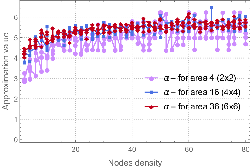
(b) Approximation value for increasing

area size

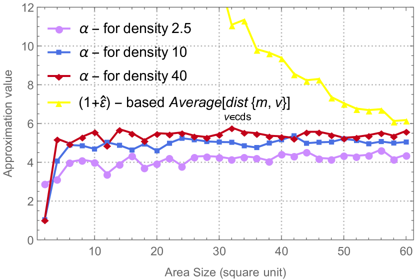
Figure 4: Simulation results for the approximation ratio $\alpha$ of Algorithm 3.

7 Conclusions and Future Work

In this work, we studied the use of data MULEs in order to gather data and increase information survivability in wireless sensor networks. We considered the MULE problem for a general UDG with a single MULE and only one failed sensor, and referred to this problem as $\left(1,1\right)-MULE-UDG$. We showed that with a reasonable assumption it can be reduced to a MWCDS problem with an approximation of $\left(1+\varepsilon\right)$. Then, we proposed a primal-dual algorithm that finds a $20-approximate$ solution to the reduced problem of MWCDS in polynomial time. Finally, we introduced the complete algorithm which produces a $\left(20+\varepsilon\right)$-approximate solution for the $\left(1,1\right)-MULE-UDG$ problem in $O\left(n^{3}\cdot\varDelta\left(G\right)\right)$ time. Also, we have shown by simulation that in practice the algorithm achieves even better results. Future extensions of our work could investigate how to expand the algorithm for multiple MULEs in the network, or for different cost functions. In addition, it will be interesting to explore the implications of the algorithm technique on the research field of the MWCDS problem.

Acknowledgements: The research has been supported by Israel Science Foundation grant No. 317/15 and the US Army Research Office under grant #W911NF-18-1-0399.

References

- [1] Stav Ashur. Data gathering in faulty sensor networks using a mule. In 34th European Workshop on Computational Geometry (EuroCG ’18), March 2018.
- [2] Brent N. Clark, Charles J. Colbourn, and David S. Johnson. Unit disk graphs. Discrete Mathematics, 86(1):165 – 177, December 1990.
- [3] Jon Crowcroft, Liron Levin, and Michael Segal. Using data mules for sensor network data recovery. Ad Hoc Networks, 40:26 – 36, 2016.
- [4] G. B. Dantzig, L. R. Ford, and D. R. Fulkerson. A primal-dual algorithm. May 1956.
- [5] Thomas Erlebach and Matúš Mihalák. A (4+)-approximation for the minimum-weight dominating set problem in unit disk graphs. In Approximation and Online Algorithms, pages 135–146. Springer Berlin Heidelberg, 2010.
- [6] M. Goemans and D. Williamson. A general approximation technique for constrained forest problems. SIAM Journal on Computing, 24(2):296–317, 1995.
- [7] M. X. Goemans and D. P. Williamson. The primal-dual method for approximation algorithms and its application to network design problems, 1997.
- [8] Liron Levin, Alon Efrat, and Michael Segal. Collecting data in ad-hoc networks with reduced uncertainty. Ad Hoc Networks, 17:71–81, jun 2014.
- [9] Satish B. Rao and Warren D. Smith. Approximating geometrical graphs via "spanners" and "banyans". In Proceedings of the thirtieth annual ACM symposium on Theory of computing - 98. ACM Press, 1998.
- [10] Rahul C. Shah, Sumit Roy, Sushant Jain, and Waylon Brunette. Data mules: modeling a three-tier architecture for sparse sensor networks. In Proceedings of the First IEEE International Workshop on Sensor Network Protocols and Applications, 2003., pages 30–41, May 2003.
- [11] Arun A. Somasundara, Aditya Ramamoorthy, and Mani B. Srivastava. Mobile element scheduling for efficient data collection in wireless sensor networks with dynamic deadlines. In IEEE International Real-Time Systems Symposium, number 25th. IEEE, December 2004.
- [12] David P. Williamson. The primal-dual method for approximation algorithms. Mathematical Programming, 91(3):447–478, Feb 2002.
- [13] Weili Wu, Hongwei Du, Xiaohua Jia, Yingshu Li, and Scott C.-H. Huang. Minimum connected dominating sets and maximal independent sets in unit disk graphs. Theoretical Computer Science, 352(1-3):1–7, mar 2006.
- [14] Harel Yedidsion, Aritra Banik, Paz Carmi, Matthew J. Katz, and Michael Segal. Efficient data retrieval in faulty sensor networks using a mobile mule. In 2017 15th International Symposium on Modeling and Optimization in Mobile, Ad Hoc, and Wireless Networks (WiOpt), number 15th, pages 1–8. IEEE, may 2017.
- [15] Feng Zou, Yuexuan Wang, Xiao-Hua Xu, Xianyue Li, Hongwei Du, Pengjun Wan, and Weili Wu. New approximations for minimum-weighted dominating sets and minimum-weighted connected dominating sets on unit disk graphs. Theoretical Computer Science, 412(3):198–208, jan 2011.