Permutation-Based Causal Structure Learning
with Unknown Intervention Targets

Abstract

We consider the problem of estimating causal DAG models from a mix of observational and interventional data, when the intervention targets are partially or completely unknown. This problem is highly relevant for example in genomics, since gene knockout technologies are known to have off-target effects. We characterize the interventional Markov equivalence class of DAGs that can be identified from interventional data with unknown intervention targets. In addition, we propose a provably consistent algorithm for learning the interventional Markov equivalence class from such data. The proposed algorithm greedily searches over the space of permutations to minimize a novel score function. The algorithm is nonparametric, which is particularly important for applications to genomics, where the relationships between variables are often non-linear and the distribution non-Gaussian. We demonstrate the performance of our algorithm on synthetic and biological datasets. Links to an implementation of our algorithm and to a reproducible code base for our experiments can be found at https://uhlerlab.github.io/causaldag/utigsp.

1 INTRODUCTION

Causal models are a prerequisite for answering scientific, sociological, and technological questions across disciplines (Friedman et al., 2000; Pearl, 2000; Robins and Hernan, 2000; Spirtes et al., 2000); examples are “what genetic activity is responsible for cancer?” or “what is the effect on unemployment of raising minimum wage?”. This necessity has generated intense interest in causal structure learning, i.e., the problem of learning a causal graphical model that represents the causal relationships of different elements in a complex system from data. Typically, the causal model is in the form of a directed acyclic graph (DAG).

Since different causal DAG models can generate the same observational distribution, a DAG is in general only identifiable up to its Markov equivalence class (MEC) from observational data (Verma and Pearl, 1990). Interventional data is necessary for reducing the ambiguity. Given observational and interventional data the identifiability of the underlying causal DAG model improves to a smaller equivalence class known as the $\mathcal{I}$-MEC (Hauser and Bühlmann, 2012; Yang et al., 2018). With the advent of gene editing technologies in genomics, high-throughput interventional gene expression data is being produced (Dixit et al., 2016). Therefore, an important problem in this field is to fully utilize such data to infer the finest equivalence class of causal DAGs describing the data. This is made particularly challenging since gene knockout experiments are known to have severe off-target effects, i.e., the CRISPR-Cas gene-editing technology performs cleavage at unknown genome sites other than their intended target (Fu et al., 2013; Wang et al., 2015). Not accounting for these additional targets while learning causal structure leads to model misspecification, and thus incorrect conclusions. Hence it is critical to develop causal inference methods that can make use of observational and interventional data when the intervention targets are partially or completely unknown. This is the purpose of the present paper.

A variety of methods have been proposed for causal structure learning from observational and interventional data when the intervention targets are known. This includes the algorithms GIES (Hauser and Bühlmann, 2012) and IGSP (Wang et al., 2017; Yang et al., 2018) under the assumption of causal sufficiency, i.e., when there are no latent confounders, and ACI (Magliacane et al., 2016), HEJ (Hyttinen et al., 2014) and COmbINE (Triantafillou and Tsamardinos, 2015) that allow for latent confounders. Since these algorithms assume that all intervention targets are known a priori, they will in general be inconsistent in the presence of off-target effects, which may misinform downstream decision-making. To make use of interventional data with unknown intervention targets, Eaton and Murphy (2007) proposed a dynamic programming algorithm. However, it is limited both in terms of scalability and requiring parametric assumptions. A different approach to this problem is given by the invariant causal inference framework (Meinshausen et al., 2016; Rothenhäusler et al., 2015; Ghassami et al., 2017). While this approach comes with consistency guarantees, it makes various assumptions that are unlikely to hold in the context of genomics. In particular, interventions can only affect the distribution of the internal noises of the intervened targets and the functional relationship between each node and its parents is assumed to be linear. Most recently, Mooij et al. (2016) proposed the Joint Causal Inference (JCI) framework, which can be used to adapt an existing observational causal inference algorithm into a method for causal structure learning from interventional data with unknown targets. In this paper, we develop a new algorithm for learning from interventional data with unknown targets, and will also compare our algorithm to the JCI framework.

Our main contributions are as follows:

• We show that under a specific faithfulness assumption, all intervention targets are identifiable. Importantly, this implies that the degree of identifiability of the underlying causal model is the same with unknown intervention targets as when the intervention targets are known.

• By introducing a score function that is minimized by graphs in the true $\mathcal{I}$-MEC, we develop a provably consistent greedy algorithm that simultaneously learns the intervention targets as well as the $\mathcal{I}$-MEC from a mix of observational and interventional data with unknown intervention targets.

• We demonstrate the efficacy of our algorithm on synthetic and biological datasets.

2 PRELIMINARIES AND RELATED WORK

2.1 Causal DAG model

Let $\mathcal{G}=([p],\mathcal{E})$ be a directed acyclic graph (DAG) with node set $[p]:=\{1,\cdots,p\}$ and edge set $\mathcal{E}$ representing a causal model where each node $i$ is associated with a random variable $X_{i}$. Let $f$ denote the density of the data-generating distribution $\mathbb{P}$ over the random vector $X:=(X_{1},\cdots,X_{p})$. By the causal Markov property, the density function $f$ is Markov with respect to the DAG $\mathcal{G}$, i.e., the density function $f$ factorizes with respect to the DAG $\mathcal{G}$:

$$f(x)=\prod_{i\in[p]}f_{i}(x_{i}\mid x_{\operatorname{pa}_{\mathcal{G}}(i)}),$$

where $\operatorname{pa}_{\mathcal{G}}(i)$ denotes the set of nodes that are parents of $i$ in the DAG $\mathcal{G}$. A basic result for DAG models (Lauritzen, 1996, Section 3.2.2) is that $\mathbb{P}$ is Markov with respect to a DAG $\mathcal{G}$ if and only if the set of conditional independence relations in $\mathbb{P}$ is entailed by the set of d-separation statements in $\mathcal{G}$, i.e., for any disjoint sets $A$, $B$ and $C$, $X_{A}$ is conditionally independent from $X_{B}$ given $X_{C}$ whenever $A$ is d-separated from $B$ given $C$. The faithfulness assumption that is commonly assumed in existing causal inference algorithms is the assertion that the converse is also true, i.e., that the set of conditional independence relations in $\mathbb{P}$ entail all d-separation statements in $\mathcal{G}$. The main justification of the faithfulness assumption is that the Lebesgue measure of distributions unfaithful with respect to a DAG $\mathcal{G}$ is zero (Pearl, 2000).

Let $\mathcal{M}(\mathcal{G})$ denote the set of distributions that are Markov with respect to $\mathcal{G}$. Two DAGs $\mathcal{G}_{1}$ and $\mathcal{G}_{2}$ are Markov equivalent, denoted $\mathcal{G}_{1}\sim\mathcal{G}_{2}$, if $\mathcal{M}(\mathcal{G}_{1})=\mathcal{M}(\mathcal{G}_{2})$. Verma and Pearl (1990) showed that $\mathcal{G}_{1}\sim\mathcal{G}_{2}$ if and only if $\mathcal{G}_{1}$ and $\mathcal{G}_{2}$ have the same skeleton and v-structures. Moreover, if $\mathcal{G}_{1}\sim\mathcal{G}_{2}$, then $\mathcal{G}_{1}$ and $\mathcal{G}_{2}$ can be transformed to one another by a sequence of covered edge reversals, where we call an edge $i\to j$ in a DAG $\mathcal{G}$ covered if $\operatorname{pa}_{\mathcal{G}}(j)=\operatorname{pa}_{\mathcal{G}}(i)\cup\{i\}$. By a slight abuse of notation, we will also use $\mathcal{M}(\mathcal{G})$ to denote the set of DAGs that are Markov equivalent to $\mathcal{G}$, i.e., the Markov equivalence class of $\mathcal{G}$.

2.2 Interventions

Interventions on random variables can be used to improve the identifiability of the underlying causal model. A theoretical framework for modeling interventions was developed in Eberhardt and Scheines (2007). A perfect intervention assumes that all causal dependencies between intervened targets and their causes are removed (Eberhardt and Scheines, 2007). As an example, consider a perfectly performed gene knockout experiment, where the expression of a gene is set to zero and hence all interactions between gene $i$ and its upstream regulators are eliminated.

In practice, interventions often cannot fully remove the causal dependencies between an intervened target and its causes, but rather modify their causal relationship (Eberhardt and Scheines, 2007). For example, in genomics, an intervention may only inhibit the expression of a gene (Dominguez et al., 2016). Such interventions are known as imperfect. The issue of whether or not an intervention is perfect or imperfect is conceptually orthogonal to the issue of whether or not the intervention has unknown targets. For example, a chemical treatment that perfectly prevents the expression of an unknown handful of genes would be an example of a perfect intervention with unknown targets. On the other hand, injecting a cell with extra copies of mRNA from gene A would be an example of an imperfect intervention with no unknown targets, since the expression of gene A still depends on the gene regulatory network, which has not been affected. This paper is concerned with the problem of causal structure discovery from interventional data (from perfect or imperfect interventions) with unknown intervention targets.

Let $I\subseteq[p]$ denote a perfect or imperfect intervention target and let $f^{\textrm{obs}}$ and $f^{I}$ denote the densities of the observational (i.e., no interventions) and interventional distributions, respectively. A pair $(f^{\textrm{obs}},f^{I})$ is $I$-Markov with respect to a DAG $\mathcal{G}$ if $f^{\textrm{obs}}$ and $f^{I}$ are Markov with respect to $\mathcal{G}$ and for any non-intervened variable $j\in[p]\setminus I$, it holds that

$$f^{I}(x_{j}\mid x_{\operatorname{pa}_{\mathcal{G}}(j)})=f^{\textrm{obs}}(x_{j}\mid x_{\operatorname{pa}_{\mathcal{G}}(j)}),$$ (1)

i.e., the conditional distributions of the non-intervened variables are invariant across the observational and interventional distributions (Yang et al., 2018). This $I$-Markov property implies the following factorization of the interventional distribution $f^{I}$ with respect to $\mathcal{G}$:

$$f^{I}(x)=\prod_{i\not\in I}f^{\textrm{obs}}(x_{i}\mid x_{\operatorname{pa}_{\mathcal{G}}(i)})\prod_{i\in I}f^{I}(x_{i}\mid x_{\operatorname{pa}_{\mathcal{G}}(i)}).$$ (2)

Let $\mathcal{M}_{I}(\mathcal{G})$ denote the set of distributions $I$-Markov with respect to $\mathcal{G}$. Then, as in the non-interventional setting, two DAGs $\mathcal{G}_{1}$ and $\mathcal{G}_{2}$ are in the same $I$-Markov equivalence class, if $\mathcal{M}_{I}(\mathcal{G}_{1})=\mathcal{M}_{I}(\mathcal{G}_{2})$ (Hauser and Bühlmann, 2012; Yang et al., 2018).

2.3 Causal structure discovery algorithms

Causal inference algorithms can largely be categorized into three approaches, namely constraint-based methods, score-based methods, and their hybrids. Constraint-based methods, including the prominent PC algorithm (Spirtes et al., 2000), learn the causal model by treating causal inference as a constraint satisfaction problem and estimate the underlying Markov equivalence class by a sequence of conditional independence tests. Score-based methods, such as GES (Meek, 1997) and its interventional adaptation GIES (Hauser and Bühlmann, 2012), assign a score to each Markov equivalence class and learn the Markov equivalence class of the data-generating DAG by greedily optimizing a penalized likelihood score. In addition, hybrid algorithms such as GSP (Solus et al., 2017) and its interventional adaptation IGSP (Wang et al., 2017; Yang et al., 2018) have been proposed that construct a score function based on conditional independence tests. All these algorithms assume either that there is no interventional data or that the intervention targets are known. The main contributions of this paper is to provide a consistent causal inference algorithm in the setting where the intervention targets are unknown.

Recent work (Mooij et al., 2016) introduces a framework for causal structure learning using data from heterogeneous “contexts”, including data from different interventions, to which we will limit our discussion. The joint causal inference (JCI) framework associates with intervention $I_{k}$ a binary random variable ${\mathsf{I}}_{k}$, with ${\mathsf{I}}_{k}=1$ denoting that the data comes from the distribution $k$. The vector ${\mathsf{I}}$ has at most a single non-zero entry (i.e., $|{\mathsf{I}}|_{0}\leq 1$), and ${\mathsf{I}}=\mathbf{0}$ denotes that the data comes from $f^{\textrm{obs}}$. Thus, the joint distribution of the system variables $x$ and the intervention variables ${\mathsf{I}}$ is

$$f^{\textrm{joint}}(x,{\mathsf{I}})=f^{\textrm{obs}}(x)^{\mathbbm{1}_{{\mathsf{I}}=\mathbf{0}}}\prod_{k=1}^{K}f^{k}(x)^{\mathbbm{1}_{{\mathsf{I}}_{k}=1}}.$$

This distribution can be represented by the JCI-DAG, denoted $\mathcal{G}^{\textrm{joint}}_{*}$, which fuses the true underlying causal DAG $\mathcal{G}^{*}$ with a complete graph over the intervention variables, and adds the edge ${\mathsf{I}}_{k}\rightarrow x_{i}$ if $i\in I_{k}$.

To apply JCI to a causal structure learning algorithm, the algorithm must be capable of incorporating the following assumptions as background information:

• “Exogeneity”: System variables do not cause intervention variables.

• “Generic context”: The intervention variables are fully connected.

The JCI framework has been applied to a variety of constraint-based and scored-based methods, but has not been applied to any hybrid methods. In Section 4, we provide an adaptation of GSP that can incorporate the background information required for JCI, leading to a new algorithm, JCI-GSP. Then, we show that the performance of JCI-GSP suffers from treating intervention variables equivalently to system variables, and propose an improved algorithm, Unknown-Target IGSP (UT-IGSP) to overcome this problem.

3 IDENTIFIABILITY WITH UNKNOWN INTERVENTION TARGETS

In order to define consistency of a causal inference algorithm in the setting where the intervention targets are unknown, we first need to characterize the interventional Markov equivalence class in this setting. In the following, we first briefly review the graphical characterization of the interventional Markov equivalence class when all intervention targets are known and then show that the equivalence class is the same even in the setting where the intervention targets are unknown. This means that the degree of identifiability of the underlying causal DAG model is unchanged whether the intervention targets are known or unknown.

3.1 Preliminaries

We consider the setting where we have data from $K$ interventional experiments. Let $I^{k}$ denote the intervention targets of experiment $k$ and let $f^{k}$ denote the corresponding interventional distribution. We denote the full list of intervention targets by $\mathcal{I}=(I^{1},\cdots,I^{K})$. Notice that we assume throughout that we also have access to purely observational data. This assumption is satisfied in most experimental designs in practice.

The $I$-Markov property in Section 2.2 can easily be extended to the setting of multiple interventional experiments by replacing the invariance property (1) by

$$f^{k}(x_{i}\mid x_{\operatorname{pa}_{\mathcal{G}}(i)})=f^{k^{\prime}}(x_{i}\mid x_{\operatorname{pa}_{\mathcal{G}}(i)})$$

for all $k,k^{\prime}\in[K]$ and all random variables $X_{i}$ where $i\not\in I$ and $i\not\in I^{\prime}$ (see also Yang et al. (2018)). We denote the resulting $\mathcal{I}$-Markov equivalence class with respect to a DAG $\mathcal{G}$ by $\mathcal{M}_{\mathcal{I}}(\mathcal{G})$ and the equivalence relation by $\sim_{\mathcal{I}}$.

A graphical characterization of $\mathcal{I}$-Markov equivalence was provided by Yang et al. (2018). Let $\mathcal{G}^{\mathcal{I}}$ denote the DAG $\mathcal{G}$ along with additional $\mathcal{I}$-vertices $\{\zeta_{k}\}_{k\in[K]}$ and $\mathcal{I}$-edges $\{\zeta_{k}\rightarrow i\}_{i\in I^{k},I^{k}\in\mathcal{I}}$ (this is known as the interventional DAG, or $\mathcal{I}$-DAG; a concrete example is provided in Figure 1). Then $\mathcal{G}_{1}\sim_{\mathcal{I}}\mathcal{G}_{2}$ if and only if $\mathcal{G}_{1}^{\mathcal{I}}$ and $\mathcal{G}_{2}^{\mathcal{I}}$ have the same skeleton and v-structures. Similarly as in the non-interventional setting, the $\mathcal{I}$-Markov property connects the $\mathcal{I}$-DAG to invariance of conditional distributions via d-separation. Specifically, if $\{f^{k}\}_{k\in[K]}$ is $\mathcal{I}$-Markov with respect to $\mathcal{G}$, then for disjoint $A$ and $C$, $f^{I}(x_{A}\mid x_{C})=f^{\textrm{obs}}(x_{A}\mid x_{C})$ whenever $A$ and $\zeta_{I}$ are d-separated given $C\cup\zeta_{\mathcal{I}\setminus I}$, denoted as $(A\mathchoice{\mathrel{\hbox to0.0pt{$\displaystyle\perp$\hss}\mkern 2.0mu{\displaystyle\perp}}}{\mathrel{\hbox to0.0pt{$\textstyle\perp$\hss}\mkern 2.0mu{\textstyle\perp}}}{\mathrel{\hbox to0.0pt{$\scriptstyle\perp$\hss}\mkern 2.0mu{\scriptstyle\perp}}}{\mathrel{\hbox to0.0pt{$\scriptscriptstyle\perp$\hss}\mkern 2.0mu{\scriptscriptstyle\perp}}}\zeta_{I}\mid C\cup\zeta_{\mathcal{I}\setminus I})_{\mathcal{G}^{\mathcal{I}}}$. The $\mathcal{I}$-Markov equivalence class of a graph $\mathcal{G}$ can be represented by a partially directed graph, the $\mathcal{I}$-essential graph, which has a directed edge $i\rightarrow j$ in the $\mathcal{I}$-essential graph if the edge $i\to j$ is oriented in the same direction for every DAG in $\mathcal{M}_{\mathcal{I}}(\mathcal{G})$, and has an undirected edge $i-j$ if the edge is oriented in different directions for DAGs in $\mathcal{M}_{\mathcal{I}}(\mathcal{G})$.

Figure 1: The $\mathcal{I}$-DAG (left) $\mathcal{G}^{\mathcal{I}}$ and JCI-DAG (right) $\mathcal{G}^{\textrm{joint}}$ for a complete DAG and the interventions $I_{1}=\{1,2\}$ and $I_{2}=\{3\}$.

3.2 Main results

Let the estimated set of intervention targets be

$$\hat{I}^{k}=\{x_{i}\in[p]\mid f^{k}(x_{i}\mid x_{S})\neq f^{\textrm{obs}}(x_{i}\mid x_{S})~{}\forall~{}S\subseteq[p]\setminus\{i\}\}.$$

By definition, $f^{k}(x_{i}\mid x_{\operatorname{pa}_{\mathcal{G}}(i)})=f^{\textrm{obs}}(x_{i}\mid x_{\operatorname{pa}_{\mathcal{G}}(i)})$ for $i\not\in I^{k}$, so we always have $\hat{I}^{k}\subseteq I^{k}$. The following assumption ensures that $\hat{I}^{k}=I^{k}$.

Assumption 1 (Direct $\mathcal{I}$-faithfulness).

Given an interventional distribution $f^{k}$ with targets $I^{k}$, we assume that $f^{k}(x_{i}\mid x_{S})\neq f^{\textrm{obs}}(x_{i}\mid x_{S})$ for any node $i\in I^{k}$ and any subset $S\subseteq[p]\setminus\{i\}$.

This assumption rules out situations in which node $i$ has been intervened on, but there is some set $S$ for which the conditional distribution $f^{k}(x_{i}\mid x_{S})$ is unaffected. Note that this is equivalent to adjacency-faithfulness between intervention variables and their children in the JCI-DAG.

Assumption 1 is not required by known-target interventional causal inference algorithms (see for example Tian and Pearl (2001); Yang et al. (2018)). Thus, it is of interest to understand whether Assumption 1 is truly necessary for causal inference in the setting with unknown intervention targets. We end this section with the following example showing that when Assumption 1 is violated, the underlying $\mathcal{I}$-Markov equivalence class may not be identifiable, i.e., Assumption 1 is necessary for any causal inference algorithm in the setting where the intervention targets are unknown.

Example 1 (Necessity of Assumption 1).

Let $f$ be Markov to the DAG $1\rightarrow 2$ and $I_{1}=\{2\}$, with $f^{\textrm{obs}}(x_{1})=\mathcal{N}(0,1)$, $f^{\textrm{obs}}(x_{2}\mid x_{1})=\mathcal{N}(x_{1},1)$, and $f^{1}(x_{2}\mid x_{1})=\mathcal{N}(0.5x_{1},1.75)$. We have $f^{\textrm{obs}}(x_{2})=f^{1}(x_{2})=\mathcal{N}(0,2)$, violating Assumption 1. The DAG $2\rightarrow 1$ with intervention set $I^{\prime}_{1}=\{1\}$ and distributions $g^{\textrm{obs}}(x_{2})=\mathcal{N}(0,2)$, $g^{\textrm{obs}}(x_{1}\mid x_{2})=\mathcal{N}(0.5x_{2},0.5)$ and $g^{1}(x_{1}\mid x_{2})=\mathcal{N}(0.25x_{2},0.875)$ gives the same set of interventional distributions, so one cannot distinguish between the two DAGs despite the fact that they are in different interventional Markov equivalence classes.

4 ALGORITHM AND ITS CONSISTENCY

In Section 3, we have shown that the full list of intervention targets is identifiable and hence the underlying $\mathcal{I}$-MEC is the same as in the setting where all intervention targets are known. One approach for learning the $\mathcal{I}$-MEC is to first estimate $\{\hat{I}^{k}\}_{k\in[K]}$, and then apply algorithms such as IGSP (Yang et al., 2018) that operates in the setting where the intervention targets are known. However, estimating $I^{k}$ directly may require an exhaustive search over all $2^{p-1}$ subsets of variables, which is intractable for real-world applications with hundreds or thousands of nodes.

In the following, we provide a greedy algorithm that learns the $\mathcal{I}$-MEC as well as a complete list of intervention targets simultaneously. Importantly, we show that this greedy algorithm is consistent, i.e., it outputs the correct $\mathcal{I}$-MEC with increasing sample size.

4.1 Preliminaries

The proposed algorithm is an interventional adaptation of the greedy sparsest permutation (GSP) algorithm (Solus et al., 2017) that was proposed for causal inference in the purely observational setting. GSP is a permutation-based causal inference algorithm that associates a score to each permutation $\pi$, i.e., an ordering of the random variables $X_{1},\cdots,X_{p}$. It then greedily moves between permutations to optimize the given score function. More precisely, each permutation $\pi$ is associated to its minimal I-MAP, i.e., the DAG $\mathcal{G}_{\pi}:=([p],\mathcal{E}_{\pi})$ given by:

$$i\rightarrow j\in\mathcal{E}_{\pi}\;\Longleftrightarrow\;i<_{\pi}j\;\textrm{and}\quad i\not\mathchoice{\mathrel{\hbox to0.0pt{$\displaystyle\perp$\hss}\mkern 2.0mu{\displaystyle\perp}}}{\mathrel{\hbox to0.0pt{$\textstyle\perp$\hss}\mkern 2.0mu{\textstyle\perp}}}{\mathrel{\hbox to0.0pt{$\scriptstyle\perp$\hss}\mkern 2.0mu{\scriptstyle\perp}}}{\mathrel{\hbox to0.0pt{$\scriptscriptstyle\perp$\hss}\mkern 2.0mu{\scriptscriptstyle\perp}}}j\mid\operatorname{pre}_{\pi}(i,j)\setminus\{i,j\}.$$

Where $\operatorname{pre}_{\pi}(i,j)$ denotes all nodes coming before either $i$ or $j$ in the permutation $\pi$. From any starting permutation $\pi_{0}$, GSP uses a depth-first-search approach to find a new permutation $\tau$, where the moves between permutations are defined by covered edge reversals. If there exists $\tau$ obtained by a covered edge reversals such that the number of edges in the minimal I-MAP $\mathcal{G}_{\tau}$ is strictly smaller than the number of edges in $\mathcal{G}_{\pi_{0}}$, i.e., $|\mathcal{G}_{\tau}|<|\mathcal{G}_{\pi_{0}}|$, then $\pi_{0}$ is set to $\tau$ and the search continues. Otherwise, $\mathcal{M}(\mathcal{G}_{\pi_{0}})$ is returned. GSP is consistent under the faithfulness assumption, i.e., it outputs the correct Markov equivalence class in the purely observational setting (Solus et al., 2017).

4.2 Main results

Just like GSP, the proposed algorithm uses a greedy search in the space of permutations to determine the data-generating $\mathcal{I}$-MEC. Instead of using the number of edges in the minimal I-MAPs as the scoring function, we introduce a new scoring function that can make use of the interventional data without requiring knowledge of the intervention targets.

We consider the following setting: We are given the distributions $f^{\textrm{obs}},f^{1},f^{2},\cdots,f^{K}$ based on the intervention targets $\mathcal{I}:=\{I^{1},I^{2},\cdots,I^{K}\}$, which are partially known or completely unknown. For each experiment we denote any known intervention targets by $I_{\textrm{kn}}^{k}\subseteq I^{k}$. Given a permutation $\pi$ and the corresponding minimal IMAP $G_{\pi}$, we may estimate targets of interventions $k$ as follows:

$$\mathcal{I}_{\pi}^{k}=I^{k}_{\textrm{kn}}\cup\{i\mid f^{\textrm{obs}}(x_{i}\mid x_{\operatorname{pa}_{G_{\pi}}(i)})\neq f^{k}(x_{i}\mid x_{\operatorname{pa}_{G_{\pi}}(i))}\}$$

and assign the following score function:

$$S(\pi):=|\mathcal{G}_{\pi}|+\sum_{k=1}^{K}|\mathcal{I}_{\pi}^{k}|.$$

Here, $|\mathcal{G}_{\pi}|$ corresponds to the number of edges in $\mathcal{G}_{\pi}$.

To provide some intuition for the two summands in $S(\pi)$: The first summand $|\mathcal{G}_{\pi}|$ restricts the global optimum to be in the correct (observational and thus larger) MEC, while the second summand is used to further restrict the global optimum to be within the correct (interventional and thus smaller) $\mathcal{I}$-MEC. In the finite sample regime, the first summand is estimated by performing conditional independence tests using samples from just the observational distribution. The second summand is estimated by performing conditional invariance tests. In the Gaussian case, this corresponds to testing equality of regression coefficients and conditional variances, as detailed in Supplementary Material C. In the nonparametric setting, conditional invariance tests can be performed by a combination of nonparametric regression and testing for the equality of the residual distributions, as discussed in Heinze-Deml et al. (2018). The next remark provides intuition for how the second summand in the score function can pin down the correct $\mathcal{I}$-Markov equivalence class.

Remark 1 (Intuition for the score function).

Consider an interventional distribution with intervention targets $I^{k}\subseteq[p]$ based on the causal DAG $\mathcal{G}_{\pi^{*}}$. Under direct $\mathcal{I}$-faithfulness, $I_{\pi}^{k}\supseteq I^{k}$, so $S(\pi)$ is minimized if we can find $\operatorname{pa}_{G_{\pi}}(j)$ such that $f^{k}(x_{j}\mid x_{\operatorname{pa}_{\mathcal{G}_{\pi}}(j)})=f^{\textrm{obs}}(x_{j}\mid x_{\operatorname{pa}_{\mathcal{G}_{\pi}}(j)})$ for all $j\not\in I^{k}$, in which case $I_{\pi}^{k}=I^{k}$. For example, this invariance will hold if $\operatorname{pa}_{\mathcal{G}_{\pi}}(j)=\operatorname{pa}_{\mathcal{G}^{*}}(j)$. However, if $f^{k}$ is $\mathcal{I}$-faithful to $G^{\mathcal{I}}$ and there is some $j\not\in I^{k}$ such that $j$ is d-connected to $\zeta_{I_{k}}$ given $\operatorname{pa}_{\mathcal{G}_{\pi}}(j)\cup\zeta_{\mathcal{I}\setminus I_{k}}$, then $S(\pi)$ will not be minimized. In other words, minimizing the second summand may orient edges and hence increase identifiability of the underlying DAG model.

The interventional data is not only used to increase the degree of identifiability of the underlying causal model, but also to restrict the search directions in our greedy search algorithm. This is achieved by introducing a more restrictive version of a covered edge.

Definition 1.

Given a partially unknown intervention set $\mathcal{I}:=\{I^{1},\cdots,I^{K}\}$, an arrow $i\rightarrow j$ in the minimal I-MAP $\mathcal{G}_{\pi}$ is $\mathcal{I}$-covered if it is a covered arrow in $\mathcal{G}_{\pi}$ and for all $k$ such that $i\in I^{k}_{\textrm{kn}}$, it holds that $f^{k}(x_{j}\mid x_{\operatorname{pa}_{\mathcal{G}_{\pi}}(j)})\neq f^{\textrm{obs}}(x_{j}\mid x_{\operatorname{pa}_{\mathcal{G}_{\pi}}(j)})$.

Algorithm 1 Unknown-target IGSP (UT-IGSP)

Input: Distributions $f^{\textrm{obs}},f^{1},\cdots,f^{K}$ and partially known intervention sets $\mathcal{I}^{\textrm{kn}}:=\{I_{\textrm{kn}}^{1},I_{\textrm{kn}}^{2}\cdots,I_{\textrm{kn}}^{K}\}$, a starting permutation $\pi_{0}$.

Output: A permutation $\pi$ and associated minimal I-MAP $\mathcal{G}_{\pi}$, a complete set of estimated intervention targets $\mathcal{I}:=\{I^{1}_{\pi},\cdots,I^{K}_{\pi}\}$.

1. Set $\pi:=\pi_{0}$;

2. Using a depth-first search with root $\pi$, search for a permutation $\tau$ such that $S(\tau)<S(\pi)$ and that the corresponding minimal I-MAP $\mathcal{G}_{\tau}$ is connected to $\mathcal{G}_{\pi}$ by a list of $\mathcal{I}$-covered arrow reversals. If such $\tau$ exists, set $\pi$ as $\tau$ and continue this step; otherwise, return $\pi$, $\mathcal{G}_{\pi}$ and $\mathcal{I}:=\{I^{1}_{\pi},\cdots,I^{K}_{\pi}\}$.

Our proposed algorithm for causal structure discovery from interventional data with unknown or partially known intervention targets is provided in Algorithm 1 (which we name UT-IGSP for Unknown Target Interventional Greedy Sparsest Permutation Algorithm). Next, we prove consistency of this algorithm under the following assumption.

Assumption 2 ($\mathcal{I}$-faithfulness assumption).

Let $\mathcal{I}$ be a list of intervention targets. The set of distributions $\{f^{\textrm{obs}}\}\cup\{f^{I}\}_{I_{\mathcal{I}}}$ is $\mathcal{I}$-faithful with respect to a DAG $\mathcal{G}$ if $f^{\textrm{obs}}$ is faithful with respect to $\mathcal{G}$ and for any $I^{k}\in\mathcal{I}$ and disjoint $A,C\subseteq[p]$, we have that $(A\mathchoice{\mathrel{\hbox to0.0pt{$\displaystyle\perp$\hss}\mkern 2.0mu{\displaystyle\perp}}}{\mathrel{\hbox to0.0pt{$\textstyle\perp$\hss}\mkern 2.0mu{\textstyle\perp}}}{\mathrel{\hbox to0.0pt{$\scriptstyle\perp$\hss}\mkern 2.0mu{\scriptstyle\perp}}}{\mathrel{\hbox to0.0pt{$\scriptscriptstyle\perp$\hss}\mkern 2.0mu{\scriptscriptstyle\perp}}}\zeta_{k}\mid C\cup\zeta_{[K]\setminus\{k\}})_{\mathcal{G}^{\mathcal{I}}}$ if and only if $f^{k}(x_{A}\mid x_{C})=f^{\textrm{obs}}(x_{A}\mid x_{C})$.

Under the $\mathcal{I}$-Markov property it holds that $(A\mathchoice{\mathrel{\hbox to0.0pt{$\displaystyle\perp$\hss}\mkern 2.0mu{\displaystyle\perp}}}{\mathrel{\hbox to0.0pt{$\textstyle\perp$\hss}\mkern 2.0mu{\textstyle\perp}}}{\mathrel{\hbox to0.0pt{$\scriptstyle\perp$\hss}\mkern 2.0mu{\scriptstyle\perp}}}{\mathrel{\hbox to0.0pt{$\scriptscriptstyle\perp$\hss}\mkern 2.0mu{\scriptscriptstyle\perp}}}\zeta_{I}\mid C\cup\zeta_{\mathcal{I}\setminus I})_{\mathcal{G}^{\mathcal{I}}}$ implies $f^{I}(x_{A}\mid x_{C})=f^{\textrm{obs}}(x_{A}\mid x_{C})$. As in the purely observational setting, Assumption 2 gives the assertion that the converse is true. Note that the $\mathcal{I}$-faithfulness assumption is stronger than Assumption 1, but in either case, the set of distributions violating the assumption is degenerate, just as for the faithfulness assumption. Similar faithfulness assumptions have been made in prior work on learning from interventional data with known targets, in particular, Assumption 4.4 and Assumption 4.5 in Yang et al. (2018). Since our algorithm must also learn the intervention targets, it is not surprising that Assumption 2 implies both of these assumptions as special case.

Next we show that UT-IGSP (Algorithm 1) is consistent under Assumption 2. While a direct proof can be obtained and was developed in a preprint of this work, a simpler proof is now given using the JCI framework of Mooij et al. (2016). In Supplementary Material D, we also show that GSP is easily capable of handling the exogeneity and generic context assumptions described in Section 2.3 without any impact on its consistency guarantees. Hence the JCI framework can be applied to GSP, giving rise to JCI-GSP, which is described in Supplementary Material E. Compared to UT-IGSP, JCI-GSP uses estimated intervention targets in its definition of covered edges. As discussed in Remark 2 and Example 2 below, this leads JCI-GSP to be more sensitive to faithfulness violations than UT-IGSP. Consistent with this observation, UT-IGSP achieves superior performance on synthetic data as shown in Section 5.1. This motivates our introduction of UT-IGSP as the main algorithm in this paper and the use of JCI-GSP as a proof tool.

Theorem 1.

Under Assumption 2, UT-IGSP (Algorithm 1) and JCI-GSP are consistent in discovering the $\mathcal{I}$-Markov equivalence class of the data-generating DAG $\mathcal{G}_{\pi^{*}}$ as well as the set of interventional targets in each interventional distribution.

Proof.

It suffices to establish that JCI-GSP is consistent, since at each minimal I-MAP, Algorithm 1 has a superset of the search directions that JCI-GSP does. To establish consistency of JCI-GSP (i.e., that there is a weakly decreasing sequence from every minimal I-MAP of $f^{\textrm{joint}}$ to $\mathcal{G}_{\pi^{*}}$), it suffices to show that every minimal I-MAP $G^{\textrm{joint}}_{\pi}$ is a minimal I-MAP of $f^{\textrm{joint}}$.

In the construction of $G^{\textrm{joint}}_{\pi}$, we may partition the CI tests into three types:

1. between two intervention variables;

2. between an intervention variable and a system variable;

3. between two system variables;

The first type of CI test is handled by the background knowledge that the intervention variables are pairwise adjacent. Since all intervention variables are before system variables, all CI tests between intervention variables and system variables are of the form ${\mathsf{I}}_{k}\mathchoice{\mathrel{\hbox to0.0pt{$\displaystyle\perp$\hss}\mkern 2.0mu{\displaystyle\perp}}}{\mathrel{\hbox to0.0pt{$\textstyle\perp$\hss}\mkern 2.0mu{\textstyle\perp}}}{\mathrel{\hbox to0.0pt{$\scriptstyle\perp$\hss}\mkern 2.0mu{\scriptstyle\perp}}}{\mathrel{\hbox to0.0pt{$\scriptscriptstyle\perp$\hss}\mkern 2.0mu{\scriptscriptstyle\perp}}}x_{i}\mid x_{C},{\mathsf{I}}_{[K]\setminus\{k\}}$. This CI statement is equivalent to the invariance statement $f^{k}(x_{i}\mid x_{C})=f^{\textrm{obs}}(x_{i}\mid x_{C})$, so every CI test of the second type is consistent by the $\mathcal{I}$-faithfulness assumption. Finally, every CI test of the third type is consistent by the faithfulness assumption on $f^{\textrm{obs}}$, which completes the proof. ∎

Remark 2.

Note that the $\mathcal{I}$-covered edges of $\mathcal{G}_{\pi}^{\mathcal{I}}$ are a superset of the covered edges in $\mathcal{G}_{\pi}^{\textrm{joint}}$. For $i\rightarrow j$ to be covered in $\mathcal{G}_{\pi}^{\textrm{joint}}$, we must have $j\in\operatorname{ch}_{\mathcal{G}_{\pi}^{\textrm{joint}}}(\zeta_{k})$ for all $k$ such that $i\in I^{k}_{\textrm{kn}}$, i.e. $j\in I^{k}$. Then, by the definition of an intervention, $f^{k}(x_{j}\mid x_{\operatorname{pa}_{\mathcal{G}_{\pi}}(j)})\neq f^{\textrm{obs}}(x_{j}\mid x_{\operatorname{pa}_{G_{\pi}}(j)})$, so $i\rightarrow j$ is also $\mathcal{I}$-covered in $G_{\pi}^{\mathcal{I}}$. Thus, UT-IGSP always has at least as many search directions as JCI-GSP. Moreover, UT-IGSP may have strictly more search directions than JCI-GSP, and thus UT-IGSP is consistent under strictly weaker conditions than $\mathcal{I}$-faithfulness and strictly weaker conditions than required for JCI-GSP. This is demonstrated in the following example.

Example 2.

Let $\mathcal{G}=\{1\rightarrow 3,2\rightarrow 3\}$, $I^{1}=\{1\}$, and $I^{1}_{\textrm{kn}}=\emptyset$. Suppose $f^{\textrm{joint}}$ is faithful to $G^{\textrm{joint}}_{*}$ (equivalently in this case, $(f^{k})_{k\in[K]}$ is $\mathcal{I}$-faithful to $G^{\mathcal{I}}$) except that $f^{1}(x_{3})=f^{\textrm{obs}}(x_{3})$. Then in JCI-GSP, there are no reversible covered edges in $\mathcal{G}^{\textrm{joint}}_{312}$, so JCI-GSP is not consistent. However, UT-IGSP is consistent, since it may reverse $1\rightarrow 3$ to get to $\mathcal{G}^{\textrm{joint}}_{132}$, then $3\rightarrow 2$ to get to $G^{\textrm{joint}}_{*}$, as shown in Figure 2.

Our definition of $\mathcal{I}$-covered edges also differs from the definition of $\mathcal{I}$-covered edges in IGSP (for known intervention targets). In IGSP, a covered edge $i\rightarrow j$ is considered $\mathcal{I}$-covered if the marginals of $x_{j}$ are invariant, i.e., $f^{k}(x_{j})=f^{\textrm{obs}}(x_{j})$ for $k$ such that $i\in I^{k}_{\textrm{kn}}$. The IGSP definition immediately leads to problems in settings with unknown targets, since this condition is violated if $j\in I^{k}$. Furthermore, the definitions differ even in settings with no unknown targets. In both algorithms, false negatives when determining $\mathcal{I}$-covered edges are problematic, since the path to the sparsest I-MAP may be cut off. Our definition, unlike the IGSP definition, adapts to the strength of the interventions, leading to less false negatives when interventions have enough power.

Figure 2: Minimal I-MAPs $\mathcal{G}_{312}^{\textrm{joint}}$, $\mathcal{G}_{132}^{\textrm{joint}}$, and $G_{*}^{\textrm{joint}}$ from Example 2, where UT-IGSP is consistent but JCI-GSP is not.

In the following section, we will show that UT-IGSP outperforms JCI-GSP, which suggests that the consistency of UT-IGSP under weaker faithfulness conditions has an effect in the finite-sample case. We will also show that it outperforms IGSP even in settings without off-target effects, which suggests that our definition of $\mathcal{I}$-covered edges is preferable even in the known-target setting.

5 EMPIRICAL RESULTS

5.1 Simulated data

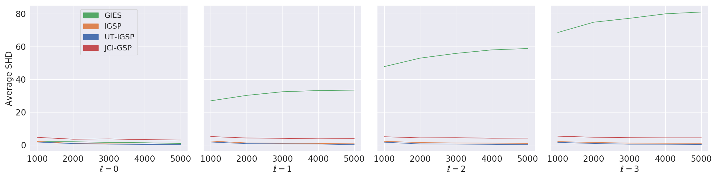
(a) Average structural Hamming distance from the true $\mathcal{I}$-essential graph

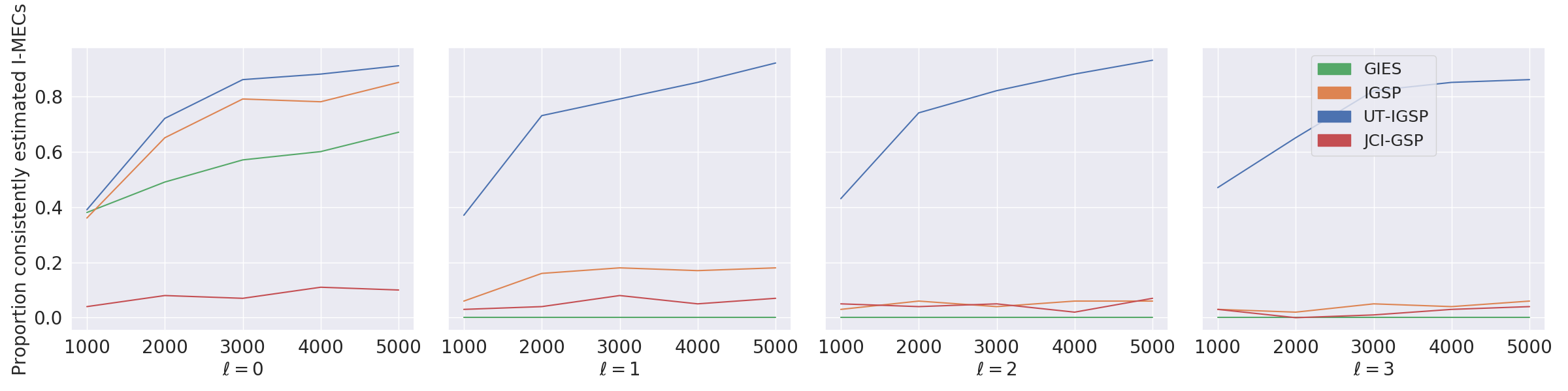
(b) Proportion of correctly estimated $\mathcal{I}$-MECs

Figure 3: Performance of different methods as a function of number of samples and number of off-target effects ($\ell$) for 100 Gaussian DAG models on 20 nodes. (a) corresponds the average Hamming distance between the estimated $\mathcal{I}$-essential graph and the true $\mathcal{I}$-essential graph, (b) corresponds to the proportions of consistently estimated $\mathcal{I}$-MECs within the 100 randomly generated Gaussian DAG models.

In this section, we compare UT-IGSP with prior algorithms that assume known intervention targets, namely GIES (Hauser and Bühlmann, 2012) and IGSP (Yang et al., 2018), and also JCI-GSP which handles unknown intervention targets, on the task of determining the $\mathcal{I}$-MEC from interventional data with partially known targets. In this simulation study, we consider data from a linear structural equation model with Gaussian noise, i.e.

$$X=W^{T}X+\epsilon,$$

where the matrix $W$ is upper-triangular with $W_{ij}\neq 0$ if and only if $i\to j\in\mathcal{G}_{\pi^{*}}$ and $\epsilon\sim\mathcal{N}(0,I_{p})$. For each simulation setting, we generated 100 realizations of Erdös-Rényi DAGs with expected neighborhood size $s=$1.5 and $p=20$ nodes. To each edge we assigned a weight $W_{ij}$ sampled independently at random from the uniform distribution on $[-1,-.25]\cup[.25,1]$, ensuring that the edge weights are bounded away from zero. For each DAG, we generated a list of intervention targets $\mathcal{I}=\{I^{1},\cdots,I^{5}\}$. We first generated known intervention targets $I^{1}_{\textrm{kn}},\cdots,I^{5}_{\textrm{kn}}$ by randomly picking $5$ nodes from the node set $[p]$ without replacement and assigning one intervention to each of $I^{1}_{\textrm{kn}},\cdots,I^{5}_{\textrm{kn}}$. Then we generated each set of unknown intervention targets $I^{k}_{\textrm{un}}$ by picking $\ell=0,\cdots,3$ nodes from the set $[p]\setminus I^{k}_{\textrm{kn}}$. Given target $I_{k}=I_{k}^{\textrm{kn}}\cup I_{k}^{\textrm{un}}$, we generated the interventional distribution via the shift intervention model. More precisely, for each node $i\in I_{k}$, we change its internal noise variance $\epsilon_{i}$ from mean 0 to mean 1. The shift in mean makes for a simple, easy-to-understand setting, and in the genetic setting, can be thought of as resulting from a gene overexpression experiment. In each study, we compared different algorithms for $n$ samples from each interventional distribution with $n=1000,~{}2000,\ldots,~{}5000$.

In each simulation, we ran GIES with its default parameters from the package pcalg. For UT-IGSP and IGSP, we chose a significance level of $\alpha=10^{-5}$.

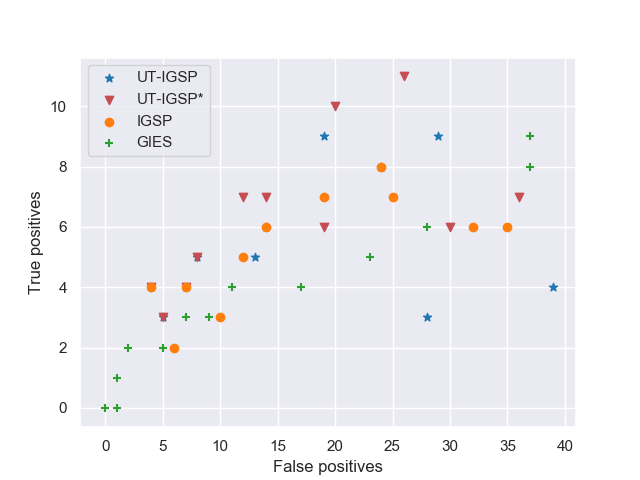
(a) Directed edge recovery

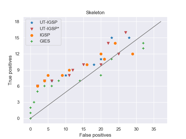
(b) Skeleton recovery

Figure 4: ROC curves for models estimated by GIES, IGSP, and UT-IGSP. UT-IGSP* indicates the results of running UT-IGSP with no intervention targets specified. The solid line corresponds to random guessing.

Figure 3 shows the structural Hamming distance (SHD) of the causal graphs estimated by each algorithm as well as the proportion of consistently estimated $\mathcal{I}$-MECs as a function of number of samples for the 4 methods. For GIES and IGSP, the $\mathcal{I}$-essential graph is with respect to known intervention targets, while for UT-IGSP, the $\mathcal{I}$-essential graph is with respect to known and estimated intervention targets. As expected, when off-target effects exist, UT-IGSP outperforms all other methods. Even with no off-target effects ($\ell=0$), UT-IGSP outperforms the other methods, suggesting that our definition of $\mathcal{I}$-covered edges combines well with sparsity-based search. JCI-GSP, although consistent as $n\to\infty$ (Theorem 1), performs poorly across all regimes. Analyzing particular cases suggests that this is due to the definition of covered edges in JCI-GSP, which allows the estimated intervention targets to drastically restrict the search space. When the conditional invariance test experiences false negatives (e.g. due to finite sample size), JCI-GSP tends to cut off paths to the true DAG. Notably, the performance of GIES degrades drastically with increasing off-target effects. In contrast, the performance of IGSP degrades only slightly, suggesting that this method is more robust to the influence of off-target effects. Results for the task of intervention target recovery and for perfect interventions are provided in Supplementary Material F. Finally, we note that UT-IGSP scales well on sparse graphs: the average runtime for the 20-node graphs considered here is below 1 second per graph, and is only 20 seconds for $p=100$, $\ell=3$, and $s=1.5$.

5.2 Biological data

We evaluated Algorithm 1 on a protein mass spectroscopy dataset acquired from cells from the human immune system (Sachs et al., 2005). The dataset contains 7466 samples measuring the abundance of phosphoproteins and phospholipids under different experimental conditions. These conditions are generated by inhibiting or activating different proteins in the protein signalling network as well as receptor enzymes via various reagents. This allows us to treat data collected from different experiments as data generated from different interventional distributions. Since some of the interventional experiments intervened on both receptor enzymes and signalling proteins and some experiments intervened only on enzymes, in this study, we define the observational dataset as the experiment for which only the receptor enzymes were perturbed, while the other 8 interventional datasets correspond to experiments where the signaling molecules have also been perturbed, as described previously in Wang et al. (2017). This division gives 1755 observational samples and 4091 interventional samples. A conventionally accepted ground-truth network is reported in Sachs et al. (2005).

In Figure 4, we plot the ROC curves of UT-IGSP, IGSP, and GIES for the true DAG and its skeleton. As expected, both IGSP and UT-IGSP outperform GIES in discovering the skeleton as well as directed edges, since they are both nonparametric approaches that allow for non-linear functional relationships. On the other hand, the performance of IGSP and UT-IGSP is comparable. This indicates that the protein signalling data collected by Sachs et al. (2005) may not contain off-target effects; consistent with the fact that these experiments were carefully designed to avoid off-target effects. In this setting, UT-IGSP does not have an advantage over the IGSP algorithm. Finally, we ran UT-IGSP without any intervention targets specified, denoted as UT-IGSP*. We found that the performance of UT-IGSP and UT-IGSP* is similar, suggesting that our algorithm may be useful in applications where off-target effects are expected.

6 DISCUSSION

In this paper, we presented a new algorithm with theoretical consistency guarantees to learn the interventional Markov equivalence class in the presence of off-target effects. We showed that the $\mathcal{I}$-Markov equivalence class is identifiable even without prior knowledge of the intervention targets, a theoretical result of independent interest (Eaton and Murphy, 2007; Meinshausen et al., 2016; Rothenhäusler et al., 2015; Ghassami et al., 2017). The application of our method to the analysis of protein signaling data suggests that it is a viable tool for biological data analysis.

Our method is of relevance beyond the analysis of interventional data in genomics. For example, our method can be used to learn causal graphs when data is generated from heterogeneous observational sources collected from naturally perturbed systems, since we can take each source as an interventional distribution with imperfect interventions and unknown intervention targets. Examples include gene expression data from normal and diseased states or stock data before and after a financial crisis. In the future, it would interesting from a theoretical and practical perspective to extend UT-IGSP to handle latent confounding and to apply UT-IGSP to other data sets.

Acknowledgements

Chandler Squires was supported by an NSF Graduate Research Fellowship and an MIT Presidential Fellowship. Caroline Uhler was partially supported by NSF (DMS-1651995), ONR (N00014-17-1-2147 and N00014-18-1-2765), IBM, a Sloan Fellowship and a Simons Investigator Award. We thank the reviewers of an early version of this paper for pointing out the connection of our algorithm to Joint Causal Inference  (Mooij et al., 2016), which we used to obtain simplified proofs of our results.

Supplementary Material

Appendix A DAG models

d-separation. For a triple of nodes $(i,j,k)$ in a graph $\mathcal{G}$ such that $i\to k\leftarrow j$, we call $k$ a collider. Given a DAG $\mathcal{G}$, we say that the two nodes $i$ and $j$ are d-connected given a set of nodes $S$ if there exists a directed path that connects $i$ and $j$ such that every non-collider on the path is not in $S$ and that for every collider $k$ on the path, we have that either $k\in S$ or some descendant of $k$ is in $S$. Given disjoint subsets $A$, $B$, and $C$, we say $A$ and $B$ are d-connected given $C$, denoted by $(A\not\mathchoice{\mathrel{\hbox to0.0pt{$\displaystyle\perp$\hss}\mkern 2.0mu{\displaystyle\perp}}}{\mathrel{\hbox to0.0pt{$\textstyle\perp$\hss}\mkern 2.0mu{\textstyle\perp}}}{\mathrel{\hbox to0.0pt{$\scriptstyle\perp$\hss}\mkern 2.0mu{\scriptstyle\perp}}}{\mathrel{\hbox to0.0pt{$\scriptscriptstyle\perp$\hss}\mkern 2.0mu{\scriptscriptstyle\perp}}}B\mid C)_{\mathcal{G}}$, if there exists a d-connecting path given $C$ between any $a\in A$ and $b\in B$. Otherwise, we say $A$ and $B$ are d-separated, denoted $(A\mathchoice{\mathrel{\hbox to0.0pt{$\displaystyle\perp$\hss}\mkern 2.0mu{\displaystyle\perp}}}{\mathrel{\hbox to0.0pt{$\textstyle\perp$\hss}\mkern 2.0mu{\textstyle\perp}}}{\mathrel{\hbox to0.0pt{$\scriptstyle\perp$\hss}\mkern 2.0mu{\scriptstyle\perp}}}{\mathrel{\hbox to0.0pt{$\scriptscriptstyle\perp$\hss}\mkern 2.0mu{\scriptscriptstyle\perp}}}B\mid C)_{\mathcal{G}}$.

Independence map. For two DAGs $\mathcal{G}$ and $\mathcal{H}$, if the set of distributions Markov with respect to $\mathcal{G}$ is a subset of the distributions Markov with respect to $\mathcal{H}$, i.e., $\mathcal{M}(\mathcal{G})\subseteq\mathcal{M}(\mathcal{H})$, we call $\mathcal{H}$ an independence map of the DAG $\mathcal{G}$, denoted as $\mathcal{G}\leq\mathcal{H}$. Based on the Markov property we can also conclude that if $\mathcal{G}\leq\mathcal{H}$, the set of conditional independence relations entailed by $\mathcal{H}$ is a subset of the conditional independence relations entailed by $\mathcal{G}$.

Appendix B Assumption 1 Incomparability

We reproduce the assumptions of Yang et al. (2018) here:

Assumption (4.4 of Yang et al. (2018)).

Let $I^{k}\in\mathcal{I}$ with $i\in I^{k}$. Then $f^{k}(x_{j})\neq f^{\textrm{obs}}(x_{j})$ for all descendants $j$ of $i$.

Assumption (4.5 of Yang et al. (2018)).

Let $I^{k}\in\mathcal{I}$ with $i\in I^{k}$. Then $f^{k}(x_{j}\mid x_{S})\neq f^{\textrm{obs}}(x_{j}\mid x_{S})$ for any child $j$ of $i$ s.t. $j\not\in I^{k}$ and for all $S\subseteq\neq_{\mathcal{G}^{*}}(j)\setminus\{i\}$, where $\neq_{\mathcal{G}^{*}}(j)$ denotes the neighbors of node $j$ in $\mathcal{G}^{*}$/

Example 2 satisfies Assumption 1. It does not satisfy Assumption 4.4, since $3$ is a descendant of $1$ but $f^{1}(x_{3})=f^{\textrm{obs}}(x_{3})$. It does not satisfy Assumption 4.5, since $3$ is a child of $1$, $S=\emptyset$ is a subset of the neighbors of $3$, and again $f^{1}(x_{3})=f^{\textrm{obs}}(x_{3})$. Thus, Assumption 1 does not imply either Assumption 4.4 or 4.5.

Let $\mathcal{G}=\{1\rightarrow 2\}$ and $I^{1}=\{2\}$. Let $f^{1}(x_{2})=f^{\textrm{obs}}(x_{2})$. Then $f$ satisfies Assumption 4.4 and 4.5, since $2$ has no children/descendants, but it does not satisfy Assumption 1. Thus, Assumption 4.4 and 4.5 do not imply Assumption 1.

Appendix C Conditional Invariance Testing

For a multivariate Gaussian distribution $f^{\textrm{obs}}$, all conditional distributions are also Gaussian, with mean given by a linear combination of the variables in the conditioning set, i.e., $X_{i}\mid X_{C}\sim\mathcal{N}(\beta_{i\mid C}X_{C}+b_{i\mid C},\sigma_{i\mid C}^{2})$. Thus, two conditional distributions $f^{1}$ and $f^{2}$ are the same if and only if the regression coefficients are the same ($H_{c}$: $\beta^{1}_{i\mid C}=\beta^{2}_{i\mid C}$ and $b^{1}_{i\mid C}=b^{2}_{i\mid C}$) and the variance are the same ($H_{v}$: $\sigma^{1}_{i\mid C}=\sigma^{2}_{i\mid C}$). By applying Bonferroni correction, to test the null hypothesis $f^{1}=f^{2}$ at significance level $\alpha$, we may test $H_{c}$ and $H_{v}$ both at significance level $\frac{\alpha}{2}$. Both $H_{c}$ and $H_{v}$ have well-known exact tests; the Chow test and F test, respectively.

Appendix D Background Knowledge in GSP

Algorithm 2 GSP

Input: Distribution $f$ and starting permutation $\pi_{0}$.

Output: A permutation $\pi$ and associated minimal I-MAP $\mathcal{G}_{\pi}$.

1. Set $\pi:=\pi_{0}$;

2. Using a depth-first search with root $\pi$, search for a permutation $\tau$ such that $S(\tau)<S(\pi)$ and that the corresponding minimal I-MAP $\mathcal{G}_{\tau}$ is connected to $\mathcal{G}_{\pi}$ by a list of $\mathcal{I}$-covered arrow reversals. If such $\tau$ exists, set $\pi$ as $\tau$ and continue this step; otherwise, return $\pi$, $\mathcal{G}_{\pi}$.

D.1 Consistency of GSP

Algorithm 2 describes the Greedy Sparsest Permutation (GSP) algorithm when there is no background information. The algorithm was originally introduced and proven to be consistent in Solus et al. (2017). We now review a simplified proof, so that we have a reference point for proving consistency after adding background knowledge.

Given a DAG $\mathcal{G}$ and an IMAP $\mathcal{H}$ of $\mathcal{G}$, a Chickering sequence from $\mathcal{G}$ to $\mathcal{H}$ is a sequence of DAGs $\mathcal{G}=\mathcal{G}_{0},\mathcal{G}_{1},\ldots,\mathcal{G}_{M-1},\mathcal{G}_{M}=\mathcal{H}$ such that $\mathcal{G}_{i}$ is an IMAP of $\mathcal{G}_{i-1}$ and $\mathcal{G}_{i}$ is obtained from $\mathcal{G}_{i-1}$ by either the addition of an edge or a covered edge reversal. Chickering (2002) proved the existence of a Chickering sequence between a DAG $\mathcal{G}$ and any IMAP $\mathcal{H}$ of $\mathcal{G}$ by repeated application of the ApplyEdgeOperation algorithm, reproduced in Algorithm 3.

Algorithm 3 ApplyEdgeOperation

Input: DAGs $\mathcal{G}$ and $\mathcal{H}$ where $\mathcal{G}\leq\mathcal{H}$ and $\mathcal{G}\neq\mathcal{H}$.

Output: A DAG $\mathcal{G}^{\prime}$ satisfying $\mathcal{G}^{\prime}\leq\mathcal{H}$ that is given by reversing an edge in $\mathcal{G}$ or adding an edge to $\mathcal{G}$.

1. Set $\mathcal{G}^{\prime}:=\mathcal{G}$.

2. While $\mathcal{G}$ and $\mathcal{H}$ contain a node $Y$ that is a sink in both DAGs and for which $\operatorname{pa}_{\mathcal{G}}(Y)=\operatorname{pa}_{\mathcal{H}}(Y)$, remove $Y$ and all incident edges from both DAGs.

3. Let $Y$ be any sink node in $\mathcal{H}$.

4. If $Y$ has no children in $\mathcal{G}$, then let $X$ be any parent of $Y$ in $\mathcal{H}$ that is not a parent of $Y$ in $\mathcal{G}$. Add the edge $X\rightarrow Y$ to $\mathcal{G}^{\prime}$ and return $\mathcal{G}^{\prime}$.

5. Let $D\in\operatorname{de}_{\mathcal{G}}(Y)$ denote the (unique) maximal element from $\operatorname{de}_{\mathcal{G}}(Y)$ within $\mathcal{H}$. Let $Z$ be any maximal child of $Y$ in $\mathcal{G}$ such that $D$ is a descendant of $Z$ in $\mathcal{G}$.

6. If $Y\rightarrow Z$ is covered in $\mathcal{G}$, reverse $Y\rightarrow Z$ in $\mathcal{G}^{\prime}$ and return $\mathcal{G}^{\prime}$.

7. If there exists a node $X$ that is a parent of $Y$ but not a parent of $Z$ in $\mathcal{G}$, then add $X\rightarrow Z$ to $\mathcal{G}^{\prime}$ and return $\mathcal{G}^{\prime}$.

8. Let $X$ be any parent of $Z$ that is not a parent of $Y$. Add $X\rightarrow Y$ to $\mathcal{G}^{\prime}$ and return $\mathcal{G}^{\prime}$.

To show that GSP is consistent, we note that $S(\pi)=|\mathcal{G}_{\pi}|$ reaches its minimum only if $\mathcal{G}_{\pi}\in\mathcal{M}(\mathcal{G}^{*})$, as shown in Solus et al. (2017). Thus, it suffices to show that from any $\pi_{0}$ s.t. $\mathcal{G}_{\pi_{0}}\not\in\mathcal{M}(\mathcal{G}^{*})$, there is some $\pi_{1}$ connected to $\pi_{0}$ by covered arrow reversals s.t. $\mathcal{G}_{\pi_{1}}$ has fewer edges than $\mathcal{G}_{\pi_{0}}$. This follows readily from the existence of the Chickering sequence: we may take the highest index DAG in the sequence that is not a minimal IMAP of $\mathcal{G}$. Such a DAG is guaranteed to exist: since $|\mathcal{G}_{\pi_{0}}|>|\mathcal{G}|$, there is at least one edge addition in the Chickering sequence.

In this section, we consider adding background knowledge of the following forms:

1. Known Adjacencies: $i$ is adjacent to node $j$.

2. Known Order Information: For the partition $U,V$ of $[p]$, $U<_{\pi^{*}}V$, i.e. if $i\in U$ and $j\in V$, then $j$ is not an ancestor of $i$ in $\mathcal{G}^{*}$.

Algorithm 4 GSP + Background

Input: Distribution $f$, starting permutation $\pi_{0}$, set of adjacent pairs $A$, partition $U,V$

Output: A permutation $\pi$ and associated minimal I-MAP $\mathcal{G}^{\textrm{bg}}_{\pi}$.

1. Set $\pi:=\pi_{0}$;

2. Using a depth-first search with root $\pi$, search for a permutation $\tau$ such that $S_{\textrm{bg}}(\tau)<S_{\textrm{bg}}(\pi)$ and that the corresponding minimal I-MAP $\mathcal{G}^{\textrm{bg}}_{\tau}$ is connected to $\mathcal{G}^{\textrm{bg}}_{\pi}$ by a list of $\mathcal{I}$-covered arrow reversals. If such $\tau$ exists, set $\pi$ as $\tau$ and continue this step; otherwise, return $\pi$, $\mathcal{G}^{\textrm{bg}}_{\pi}$.

Suppose we are given this background knowledge in the form $A=\{(i,j)\mid i\sim j\in\mathcal{G}^{*}\}$ and two sets $U$ and $V$. It is easy to adapt GSP so that its output satisfies these constraints. First, we define

$$\mathcal{G}^{\textrm{bg}}_{\pi}=\{i\rightarrow j\mid i<_{\pi}j~{}{\textrm{and}}~{}$$

$$(i\not\mathchoice{\mathrel{\hbox to0.0pt{$\displaystyle\perp$\hss}\mkern 2.0mu{\displaystyle\perp}}}{\mathrel{\hbox to0.0pt{$\textstyle\perp$\hss}\mkern 2.0mu{\textstyle\perp}}}{\mathrel{\hbox to0.0pt{$\scriptstyle\perp$\hss}\mkern 2.0mu{\scriptstyle\perp}}}{\mathrel{\hbox to0.0pt{$\scriptscriptstyle\perp$\hss}\mkern 2.0mu{\scriptscriptstyle\perp}}}j\mid\operatorname{pre}_{\pi}(\{i,j\})~{}{\textrm{or}}~{}(i,j)\in A)\}$$

Then, we define $S_{\textrm{bg}}(\pi)=\infty$ if $j<_{\pi}i$ for $i\in U$, $j\in V$, and $S_{\textrm{bg}}(\pi)=|G^{\textrm{bg}}_{\pi}|$ otherwise, and use this score in place of $S$. The modified algorithm is described in Algorithm 4.

Now we show that these adaptations retain consistency of GSP. The case of known adjacencies are simple.

Since any IMAP $\mathcal{H}$ of $\mathcal{G}^{*}$ satisfies $\operatorname{skel}(\mathcal{G}^{*})\subseteq\operatorname{skel}(\mathcal{H})$ (Raskutti and Uhler, 2018), no edge $i-j$ in $K$ is deleted over the course of GSP, i.e. not testing a CI statement between $i$ and $j$ does not change the result.

No we consider the case of known order information. We show that if $\mathcal{G}^{*}$ and $\mathcal{H}$ both satisfy the known order information, then any DAG in a Chickering sequence from $\mathcal{G}$ to $\mathcal{H}$ will satisfy the known order information, which extends to the sequence of minimal IMAPs from some starting $\mathcal{G}_{\pi}$ to $\mathcal{G}^{*}$ given in the previous section.

If $\mathcal{G}_{m}$ in the Chickering sequence satisfies the order information, there are only two scenarios in which $\mathcal{G}_{m+1}$ will not: an edge $i\rightarrow j$ with $i\in A$ and $j\in B$ is reversed, or an edge is added from $j\in B$ to $i\in A$. We will show that neither scenario happens. The ApplyEdgeOperation algorithm only reverses edges to be in the same direction as they are in $\mathcal{H}$, so the first situation never happens. The only case in which ApplyEdgeOperation adds an edge that is opposite its orientation in $\mathcal{H}$ is in Step 8: $Y$ is a sink in $\mathcal{H}$, $Z$ is a child of $Y$ in $\mathcal{G}_{m}$, and $Y\rightarrow Z$ is not covered in $\mathcal{G}_{m}$ because of a parent $X$ of $Y$ in $\mathcal{G}_{m}$ that is not a parent of $\mathcal{H}$ in $\mathcal{G}_{m}$. $\mathcal{G}_{m+1}$ violates the known order information only if $Z\in A$ and $X\in B$. We have two cases: if $Y\in A$, then $X\in A$ by the assumption that $\mathcal{G}$ satisfies the order information. If $Y\in B$, then $Z\in B$ by the assumption that $\mathcal{G}$ satisfies the known order information. Thus, in both cases, $\mathcal{G}_{m+1}$ still satisfies the known order information.

Appendix E JCI-GSP

For completeness, we outline JCI-GSP in Algorithm 5. Line 1 introduces variables $\zeta_{k}$ for each interventional setting $k\in[K]$ and lifts the distribution over $X$ to a distribution over $X$ and $\zeta$. Line 2 combines these distributions into a mixture distribution, the choice of the uniform distribution is arbitrary for the population case. With finite samples, the weights may be picked according to the number of samples from each observational/interventional setting. Line 3 forms a permutation over both $\zeta$ and $X$ by pre-pending $\pi_{0}$ with an arbitrary order of the $\zeta$ variables. Line 4 encodes the generic context background knowledge, and Line 5 encodes the background knowledge about known intervention targets. Finally, Line 7 calls GSP with the appropriate background knowledge.

Algorithm 5 JCI-GSP

Input: Distributions $f^{\textrm{obs}},f^{1},\cdots,f^{K}$ and partially known intervention sets $\mathcal{I}^{\textrm{kn}}:=\{I_{\textrm{kn}}^{1},I_{\textrm{kn}}^{2}\cdots,I_{\textrm{kn}}^{K}\}$, a starting permutation $\pi_{0}$.

Output: A permutation $\pi$ and associated minimal I-MAP $\mathcal{G}_{\pi}$, a complete set of estimated intervention targets $\mathcal{I}:=\{I^{1}_{\pi},\cdots,I^{K}_{\pi}\}$.

1. Let $g^{\textrm{obs}}=\mathbbm{1}_{\zeta=0}\otimes f^{\textrm{obs}}$, $g^{k}=\mathbbm{1}_{\zeta_{k}=1,\zeta_{\neg k}=0}\otimes f^{k}$ for $k\in[K]$.

2. Let $g=\frac{1}{K+1}(g^{\textrm{obs}}+\sum_{k\in[K]}g^{k})$

3. Set $\pi_{0}^{\prime}=\langle\zeta_{1},\ldots,\zeta_{K}\rangle\cdot\pi_{0}$

4. Set $A_{\textrm{interventions}}=\{\zeta_{i}\sim\zeta_{j}\mid i,j\in[K],i\neq j\}$

5. Set $A_{\textrm{targets}}=\cup_{k\in[K]}\{\zeta_{k}\sim i\mid i\in I_{\textrm{kn}}^{k}\}$

6. Set $A=A_{\textrm{interventions}}\cup A_{\textrm{targets}}$

7. Run GSP + Background with distribution $g$, starting permutation $\pi_{0}^{\prime}$, adjacent pairs $A$, and partition $(\zeta,X)$.

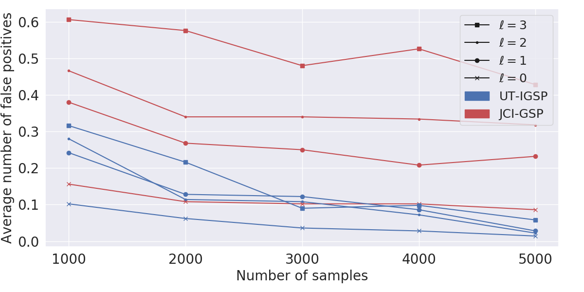
Figure 5: Performance of UT-IGSP and JCI-GSP at the task of intervention target recovery as a function of number of samples and number of off-target effects ($\ell$).

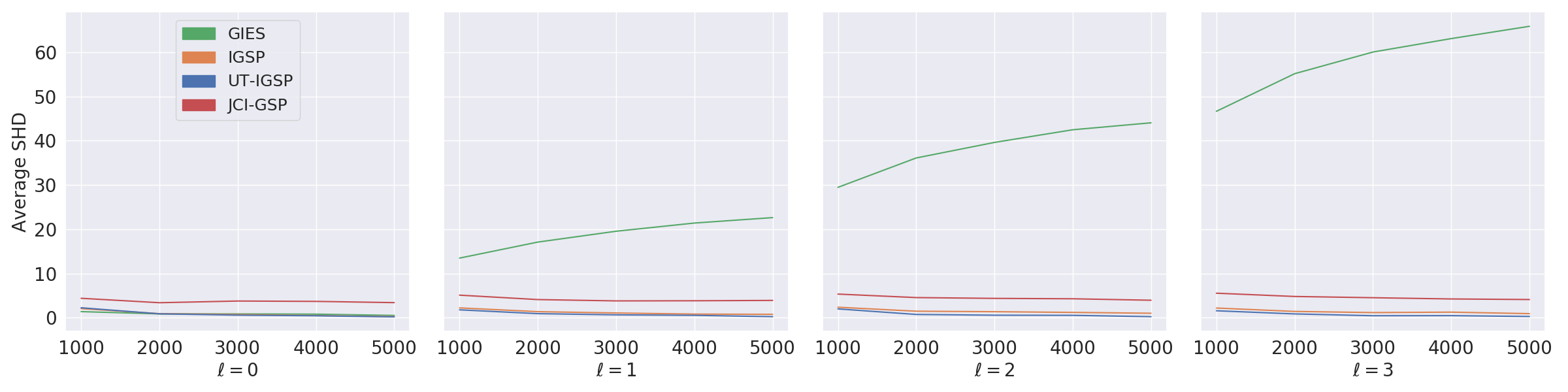
(a) Average structural Hamming distance from the true $\mathcal{I}$-essential graph

(b) Proportion of correctly estimated $\mathcal{I}$-MECs

Figure 6: Performance of different methods as a function of number of samples and number of off-target effects ($\ell$) for 100 Gaussian DAG models on 20 nodes. (a) corresponds the average Hamming distance between the estimated $\mathcal{I}$-essential graph and the true $\mathcal{I}$-essential graph, (b) corresponds to the proportions of consistently estimated $\mathcal{I}$-MECs within the 100 randomly generated Gaussian DAG models.

Appendix F Additional Evaluation

F.1 Intervention Recovery

In Fig. 5, we use the same data generated in Section 5.1, and report the number of false positive intervention targets for UT-IGSP. The average number of false negatives was negligble ($<.04$) for both methods.

F.2 Perfect Interventions

In this section, we sample Gaussian DAG models and intervention targets in the same manner as described in Section 5.1. However, instead of using shift interventions, we use perfect interventions. In particular, for $i\in I^{k}$, we completely remove the dependency between an intervened node and its parents (i.e., set $B_{ji}=0$ for $j\in\operatorname{pa}_{\mathcal{G}^{*}}(i)$), and change its internal noise variance to $\epsilon_{i}\sim\mathcal{N}(1,0.1)$. GIES was designed specifically for learning from perfect interventions, making perfect interventions a more fair comparison than shift interventions. Indeed, GIES performs better when $\ell=0$ than it did for shift interventions, even outperforming UT-IGSP when $n=1,000$. However, the overall trends remain: UT-IGSP outperforms GIES when the number of samples becomes large, and the performance of GIES is drastically reduced by even a single off-target intervention.

References

- Chickering (2002) D. M. Chickering. Optimal structure identification with greedy search. Journal of Machine Learning Research, 3(Nov):507–554, 2002.
- Dixit et al. (2016) A. Dixit, O. Parnas, B. Li, et al. Perturb-seq: dissecting molecular circuits with scalable single-cell RNA profiling of pooled genetic screens. Cell, 167(7):1853–1866, 2016.
- Dominguez et al. (2016) A. A. Dominguez, W. A. Lim, and L. S. Qi. Beyond editing: repurposing CRISPR–Cas9 for precision genome regulation and interrogation. Nature Reviews Molecular Cell Biology, 17(1):5, 2016.
- Eaton and Murphy (2007) D. Eaton and K. Murphy. Exact Bayesian structure learning from uncertain interventions. In Artificial Intelligence and Statistics, pages 107–114, 2007.
- Eberhardt and Scheines (2007) Frederick Eberhardt and Richard Scheines. Interventions and causal inference. Philosophy of Science, 74(5):981–995, 2007.
- Friedman et al. (2000) N. Friedman, M. Linial, I. Nachman, and D. Pe’er. Using Bayesian networks to analyze expression data. Journal of Computational Biology, 7(3-4):601–620, 2000.
- Fu et al. (2013) Y. Fu, J. A. Foden, C. Khayter, et al. High-frequency off-target mutagenesis induced by CRISPR-Cas nucleases in human cells. Nature Biotechnology, 31(9):822, 2013.
- Ghassami et al. (2017) A. Ghassami, S. Salehkaleybar, N. Kiyavash, and K. Zhang. Learning causal structures using regression invariance. In Advances in Neural Information Processing Systems, pages 3011–3021, 2017.
- Hauser and Bühlmann (2012) A. Hauser and P. Bühlmann. Characterization and greedy learning of interventional Markov equivalence classes of directed acyclic graphs. Journal of Machine Learning Research, 13(Aug):2409–2464, 2012.
- Heinze-Deml et al. (2018) C. Heinze-Deml, J. Peters, and N. Meinshausen. Invariant causal prediction for nonlinear models. Journal of Causal Inference, 6(2), 2018.
- Hyttinen et al. (2014) A. Hyttinen, F. Eberhardt, and M. Järvisalo. Constraint-based causal discovery: Conflict resolution with answer set programming. In Proceedings of the 30th Conference on Uncertainty in Artificial Intelligence, pages 340–349, 2014.
- Lauritzen (1996) S. L Lauritzen. Graphical Models. Clarendon Press, 1996.
- Magliacane et al. (2016) S. Magliacane, T. Claassen, and J. M. Mooij. Ancestral causal inference. In Advances in Neural Information Processing Systems, pages 4466–4474, 2016.
- Meek (1997) C. Meek. Graphical Models: Selecting Causal and Statistical Models. PhD thesis, Carnegie Mellon University, 1997.
- Meinshausen et al. (2016) N. Meinshausen, A. Hauser, J. M. Mooij, J. Peters, P. Versteeg, and P. Bühlmann. Methods for causal inference from gene perturbation experiments and validation. Proceedings of the National Academy of Sciences, 113(27):7361–7368, 2016.
- Mooij et al. (2016) J. M. Mooij, S. Magliacane, and T. Claassen. Joint causal inference from multiple contexts. Preprint arXiv:1611.10351, 2016.
- Pearl (2000) J. Pearl. Causality: Models, Reasoning, and Inference. Cambridge University Press, 2000.
- Raskutti and Uhler (2018) G. Raskutti and C. Uhler. Learning directed acyclic graph models based on sparsest permutations. Stat, 7(1):e183, 2018.
- Robins and Hernan (2000) J. M. Robins and B. Hernan, Miguel. A.and Brumback. Marginal structural models and causal inference in epidemiology, 2000.
- Rothenhäusler et al. (2015) D. Rothenhäusler, C. Heinze, J. Peters, and N. Meinshausen. Backshift: Learning causal cyclic graphs from unknown shift interventions. In Advances in Neural Information Processing Systems, pages 1513–1521, 2015.
- Sachs et al. (2005) K. Sachs, O. Perez, D. Pe’er, D. A. Lauffenburger, and G. P. Nolan. Causal protein-signaling networks derived from multiparameter single-cell data. Science, 308(5721):523–529, 2005.
- Solus et al. (2017) L. Solus, Y. Wang, L. Matejovicova, and C. Uhler. Consistency guarantees for permutation-based causal inference algorithms. Preprint arXiv:1702.03530, 2017.
- Spirtes et al. (2000) P. Spirtes, C. N. Glymour, and R. Scheines. Causation, Prediction, and Search. MIT press, 2000.
- Tian and Pearl (2001) J. Tian and J. Pearl. Causal discovery from changes. In Proceedings of the 17th Conference on Uncertainty in Artificial Intelligence, pages 512–521, 2001.
- Triantafillou and Tsamardinos (2015) S. Triantafillou and I. Tsamardinos. Constraint-based causal discovery from multiple interventions over overlapping variable sets. Journal of Machine Learning Research, 16:2147–2205, 2015.
- Verma and Pearl (1990) T. Verma and J. Pearl. Equivalence and synthesis of causal models. In Proceedings of the Sixth Annual Conference on Uncertainty in Artificial Intelligence, pages 255–270, 1990.
- Wang et al. (2015) X. Wang, Y. Wang, X. Wu, et al. Unbiased detection of off-target cleavage by CRISPR-Cas9 and TALENs using integrase-defective lentiviral vectors. Nature Biotechnology, 33(2):175, 2015.
- Wang et al. (2017) Y. Wang, L. Solus, K. Yang, and C. Uhler. Permutation-based causal inference algorithms with interventions. In Advances in Neural Information Processing Systems, pages 5822–5831, 2017.
- Yang et al. (2018) K. D. Yang, A. Katcoff, and C. Uhler. Characterizing and learning equivalence classes of causal DAGs under interventions. In Proceedings of Machine Learning Research, volume 80, pages 5537–5546, 2018.