PushTASEP in inhomogeneous space

Abstract.

We consider the PushTASEP (pushing totally asymmetric simple exclusion process, also sometimes called long-range TASEP) with the step initial configuration evolving in an inhomogeneous space. That is, the rate of each particle’s jump depends on the location of this particle. We match the distribution of the height function of this PushTASEP with Schur processes. Using this matching and determinantal structure of Schur processes, we obtain limit shape and fluctuation results which are typical for stochastic particle systems in the Kardar-Parisi-Zhang universality class. PushTASEP is a close relative of the usual TASEP. In inhomogeneous space the former is integrable, while the integrability of the latter is not known.

1. Introduction and main results

1.1. Overview

The totally asymmetric simple exclusion process (TASEP) was introduced about 50 years ago, independently in biology [MGP68], [MG69] and probability theory [Spi70]. The latter paper also introduced zero-range processes and long-range TASEP. The long-range TASEP (which we call PushTASEP following more recent works) is the focus of the present paper.

Since early works, TASEP and PushTASEP were often studied in parallel. Once a result (such as description of hydrodynamics and local equilibria [Lig05], limiting density [Ros81], or asymptotic fluctuations [Joh00]) for TASEP is established, it can often be generalized to PushTASEP using similar tools. See [DLSS91] for hydrodynamics and related results for the PushTASEP (viewed as a special case of the Toom’s model), and, e.g., [DW08], [BF08] for fluctuation results. Borodin and Ferrari [BF14] introduced a two-dimensional stochastic particle system whose two different one-dimensional (marginally Markovian) projections are TASEP and PushTASEP. This coupling works best for special examples of initial data, most notably, for step initial configurations. It is worth pointing out that most known asymptotic fluctuation results for TASEP, PushTASEP, and related systems (in the Kardar-Parisi-Zhang universality class, cf. [Cor12], [QS15]) require integrability, that is, the presence of some exact formulas in the pre-limit system.

Running either TASEP or PushTASEP in inhomogeneous space (such that the particles’ jump rates depend on their locations) is a natural generalization. Hydrodynamic approach works well in macroscopically inhomogeneous systems, and allows to write down PDEs for limiting densities [Lan96], [Sep99], [RT08], [GKS10], [Cal15]. This leads to law of large numbers type results for the height function (in particular, of the inhomogeneous TASEP). However, when the disorder is microscopic (such as just one slow bond), this affects the local equilibria, and makes the analysis of both limit shape and asymptotic fluctuations of TASEP much harder [BSS14], [BSS17]. Overall, putting TASEP on inhomogeneous space breaks its integrability.

On the other hand, considering particle-dependent inhomogeneity (when the jump rate depends on the particle’s number, but not its location) in TASEP preserves its integrability, and allows to extract the corresponding fluctuation results, cf. [Bai06], [BFS09], [Dui13].

The main goal of this paper is to show that, in contrast with TASEP, the PushTASEP in inhomogeneous space started from the step initial configuration retains the integrability for arbitrary inhomogeneities. Namely, we obtain a matching of the PushTASEP to a certain Schur process, which follows by taking a third marginally Markovian projection of the two-dimensional dynamics of Borodin–Ferrari [BF14], which was not observed previously. This coupling is also present in the Robinson-Schensted-Knuth insertion — a mechanism originally employed to obtain TASEP fluctuations in [Joh00]. The coupling of inhomogeneous PushTASEP to Schur processes, together with their determinantal structure [Oko01], [OR03] leads to exact formulas for the PushTASEP. We illustrate the integrability by obtaining limit shape and fluctuation results for PushTASEP with arbitrary macroscopic inhomogeneity.

Remark 1.1.

Based on the tools employed in the present work, one can even say that our results could have been observed already in the mid-2000s. However, it is the much more recent development of stochastic vertex models, especially their couplings in [BBW18], [BM18], [BP19] to Hall-Littlewood processes, that prompted the present work (as a $t=0$ degeneration of the Hall-Littlewood situation). Asymptotic behavior of the Hall-Littlewood deformation of the PushTASEP (in a homogeneous case) was studied in [Gho17].

Other examples of integrable stochastic particle systems in one-dimensional inhomogeneous space have been recently studied in [BP18], [KPS19]. These systems may be viewed as analogues of $q$-TASEP or TASEP, respectively in continuous space. (The $q$-TASEP is a certain integrable $q$-deformation of TASEP [BC14].) In those inhomogeneous systems, a certain choice of inhomogeneity leads to interesting phase transitions corresponding to formation of “traffic jams”, when the density goes to infinity. In PushTASEP the density is bounded by one, and so we do not expect this type of phase transitions to appear. A two-dimensional stochastic particle system in inhomogeneous space unifying both the inhomogeneous PushTASEP considered in the present paper, and a TASEP-like process similar to the one in [KPS19], is studied in [Ass20] (the latter was completed simultaneously with the present paper and independently of it).

In the rest of the introduction we give the main definitions and formulate the results.

1.2. PushTASEP in inhomogeneous space

Fix a positive speed function $\xi_{\bullet}=\{\xi_{x}\}_{x\in\mathbb{Z}_{\geq 1}}$, uniformly bounded away from zero and infinity. By definition, the PushTASEP is a continuous time Markov process on particle configurations

$$\mathsf{x}_{1}(t)<\mathsf{x}_{2}(t)<\mathsf{x}_{3}(t)<\ldots$$ (1.1)

on $\mathbb{Z}_{\geq 1}$ (at most one particle per site is allowed). We consider only the step initial configuration $\mathsf{x}_{i}(0)=i$ for all $i\geq 1$, so at all times the particle configuration has a leftmost particle.

The system evolves as follows. At each site $x\in\mathbb{Z}_{\geq 1}$ there is an independent exponential clock with rate $\xi_{x}$ (i.e., the mean waiting time till the clock rings is $1/\xi_{x}$). When the clock at site $x\in\mathbb{Z}_{\geq 1}$ rings and there is no particle at $x$, nothing happens. Otherwise, let some particle $\mathsf{x}_{i}$ be at $y$. When the clock rings, $\mathsf{x}_{i}$ jumps to the right by one. If the destination $x+1$ is occupied by $\mathsf{x}_{i+1}$, then $\mathsf{x}_{i+1}$ is pushed to the right by one, which may trigger subsequent instantaneous pushes. That is, if there is a packed cluster of particles to the right of $\mathsf{x}_{i}$, i.e., $\mathsf{x}_{i+m}-m=\ldots=\mathsf{x}_{i+1}-1=\mathsf{x}_{i}$ and $\mathsf{x}_{i+m+1}-1>\mathsf{x}_{i+m}$ for some $m\in\left\{1,2,\ldots\right\}\cup\left\{+\infty\right\}$, then each of the particles $\mathsf{x}_{i+\ell}$, $\ell=1,\ldots,m$, is instantaneously pushed to the right by one. The case $m=+\infty$ corresponds to pushing the whole right-infinite densely packed cluster of particles to the right by one. Clearly, the evolution preserves the order (1.1) of particles. See Figure 1 for an illustration.

Figure 1. Two possible transitions in the inhomogeneous PushTASEP. The first one corresponds to activating the particle at $3$ which happens at rate $\xi_{3}$. This particle then pushes two other particles (located at $4$ and $5$) to the right by one. The second transition corresponds to activating the particle at $12$ at rate $\xi_{12}$.

Thus described Markov process on particle configurations in $\mathbb{Z}_{\geq 1}$ is well-defined. Indeed, consider its restriction to $\left\{1,\ldots,N\right\}\subset\mathbb{Z}_{\geq 1}$ for any $N$. This is a continuous time Markov process on a finite space in which at most one exponential clock can ring at a given time moment. For different $N$, such restrictions are compatible, and thus the process on configurations in $\mathbb{Z}_{\geq 1}$ exists by the Kolmogorov extension theorem. Note however that the number of jumps in the process on $\mathbb{Z}_{\geq 1}$ during each initial time interval $[0,\varepsilon)$, $\varepsilon>0$, is infinite.

Remark 1.2.

The PushTASEP on the whole space $\mathbb{Z}_{\geq 1}$ might be alternatively described as follows. When a particle jumps, it goes to the closest empty site that is to its right. If there are no empty sites to the right, the particle disappears.

1.3. Determinantal structure

The height function of the PushTASEP is defined as

$$h(t,N):=\#\{\textnormal{particles in $\left\{1,\ldots,N\right\}$ at time $t$}\},\qquad N\in\mathbb{Z}_{\geq 1},\quad t\in\mathbb{R}_{\geq 0}.$$ (1.2)

The step initial condition corresponds to $h(0,N)=N$ for all $N\geq 0$.

Definition 1.3.

A down-right path in the $(t,N)$ plane is a collection $\mathfrak{p}=\{(t_{i},N_{i})\}_{i=1}^{r}$, where $r\geq 1$,

$$N_{1}\geq N_{2}\geq\ldots\geq N_{r}\geq 0,\qquad 0\leq t_{1}\leq t_{2}\leq\ldots\leq t_{r},$$ (1.3)

and the points $(t_{i},N_{i})$ are pairwise distinct.

Remark 1.4.

Down-right paths are also called space-like (as opposed to time-like, when both $t_{i}$ and $N_{i}$ increase). These names come from a growth model reformulation, cf. [DLSS91], [Fer08].

Define a kernel depending on the speed function $\xi_{\bullet}$ by

$$K(t,N,x;t^{\prime},N^{\prime},x^{\prime}):=\mathbf{1}_{t=t^{\prime}}\mathbf{1}_{N=N^{\prime}}\mathbf{1}_{x=x^{\prime}}-\frac{1}{(2\pi\mathbf{i})^{2}}\oint\oint\frac{dz\,dw}{z-w}\frac{w^{x^{\prime}+N^{\prime}}}{z^{x+N+1}}\,e^{tz-t^{\prime}w}\frac{\prod_{a=1}^{N}\bigl{(}z-\xi_{a}\bigr{)}}{\prod_{b=1}^{N^{\prime}}\bigl{(}w-\xi_{b}\bigr{)}}.$$ (1.4)

The integration contours are positively oriented simple closed curves around $0$, the $w$ contour additionally encircles all $\{\xi_{x}\}_{x\in\mathbb{Z}_{\geq 1}}$, and the contours satisfy $|z|>|w|$ for $t\leq t^{\prime}$ and $|z|<|w|$ for $t>t^{\prime}$. (Throughout the text $\mathbf{1}_{A}$ stands for the indicator of $A$, which is $1$ if condition $A$ is true, and is $0$ otherwise. By $\mathbf{1}$ without subscripts we will also mean the identity operator.)

Fix a down-right path $\mathfrak{p}=\{(t_{i},N_{i})\}_{i=1}^{r}$, and define the space

$$\mathcal{X}:=\mathcal{X}_{1}\sqcup\ldots\sqcup\mathcal{X}_{r},\qquad\mathcal{X}_{i}=\mathbb{Z}.$$

For $y\in\mathcal{X}_{i}$ set $t(y)=t_{i}$, $N(y)=N_{i}$.

Definition 1.5.

We define a determinantal random point process $\mathfrak{L}_{\mathfrak{p}}$ on $\mathcal{X}$ with the correlation kernel expressed through $K$ of (1.4). Namely, for any $m\geq 1$ and any pairwise distinct $y^{1},\ldots y^{m}\in\mathcal{X}$, let the corresponding correlation function of $\mathfrak{L}_{\mathfrak{p}}$ be given by

$$\mathbb{P}\left(\textnormal{$\mathfrak{L}_{\mathfrak{p}}$ contains all of $y^{1},\ldots,y^{m}$}\right)=\mathop{\mathrm{det}}_{i,j=1}^{m}\Bigl{[}K\bigl{(}t(y^{i}),N(y^{i}),y^{i};t(y^{j}),N(y^{j}),y^{j}\bigr{)}\Bigr{]}.$$ (1.5)

The process $\mathfrak{L}_{\mathfrak{p}}$ exists because it corresponds to column lengths in a certain specific Schur process, see Section 2 for details. The Schur process interpretation also implies that on each $\mathcal{X}_{i}=\mathbb{Z}$ the random point configuration $\mathfrak{L}_{\mathfrak{p}}$ almost surely has a leftmost point. Denote it by $\widehat{\ell}(t_{i},N_{i})$.

The joint distribution of the leftmost points $\{\widehat{\ell}(t_{i},N_{i})\}$ is identified with the inhomogeneous PushTASEP. The following theorem is the main structural result of the present paper.

Theorem 1.6.

Fix an arbitrary down-right path $\mathfrak{p}=\{(t_{i},N_{i})\}_{i=1}^{r}$. The joint distribution of the PushTASEP height function along this down-right path is related to the determinantal process $\mathfrak{L}_{\mathfrak{p}}$ defined above as

$$\bigl{\{}h(t_{i},N_{i})\bigr{\}}_{i=1}^{r}\stackrel{{\scriptstyle d}}{{=}}\bigl{\{}N_{i}+\widehat{\ell}(t_{i},N_{i})\bigr{\}}_{i=1}^{r},$$

where “ $\stackrel{{\scriptstyle d}}{{=}}$” means equality in distribution.

Corollary 1.7.

For any $t\geq 0$, $N\geq 1$, and $y\geq 0$ we have

$$\begin{split}\mathbb{P}\bigl{(}h(t,N)>y\bigr{)}&=\det\bigl{(}\mathbf{1}-K(t,N,\cdot;t,N,\cdot)\bigr{)}_{\left\{\ldots,y-N-2,y-N-1,y-N\right\}}\\ &=1+\sum_{n=1}^{\infty}\frac{(-1)^{n}}{n!}\sum_{x_{1}=-\infty}^{y-N}\ldots\sum_{x_{n}=-\infty}^{y-N}\;\mathop{\mathrm{det}}_{i,j=1}^{n}\left[K(t,N,x_{i};t,N,x_{j})\right],\end{split}$$ (1.6)

where the second equality is the series expansion of the Fredholm determinant given in the first equality. (See Section 2.8 below for more details on Fredholm determinants.) Similar Fredholm determinantal formulas are available for joint distributions of the PushTASEP height function along down-right paths.

Theorem 1.6 is a restatement of a known result on how Schur processes appear in stochastic interacting particle systems in $(2+1)$ dimensions. Via Robinson-Schensted-Knuth (RSK) correspondences, such connections can be traced to [VK86], and they were heavily utilized in probabilistic context starting from [BDJ99], [Joh00], [PS02]. Markov dynamics on particle configurations coming from RSK correspondences were studied in [Bar01], [O’C03b], [O’C03a]. Another type of Markov dynamics whose fixed-time distributions are given by Schur processes was introduced in [BF14], and it, too, can be utilized to obtain Theorem 1.6. A self-contained exposition of the proof of this theorem following the latter approach is presented in Section 2.

Remark 1.8 (Connection to vertex models).

Yet another alternative way of getting Theorem 1.6 is to view the PushTASEP as a degeneration of the stochastic six vertex model [GS92], [BCG16]. The latter was recently connected to Hall-Littlewood processes [Bor18], [BBW18], [BM18]. Setting the Hall-Littlewood parameter $t$ to zero leads to a distributional mapping between our inhomogeneous PushTASEP and Schur processes.

1.4. Hydrodynamics

Let the space and time in the PushTASEP, as well as the speed function scale as follows:

$$t=\tau L,\qquad N=\lfloor\eta L\rfloor,\qquad\xi_{x}=\boldsymbol{\xi}(x/L),\quad x\in\mathbb{Z}_{\geq 1},$$ (1.7)

where $L$ is the large parameter going to infinity, and $\boldsymbol{\xi}(\cdot)$ is a fixed positive limiting speed function bounded away from zero and infinity. Under (1.7), one expects that the height function $h(t,N)$ admits a limit shape (i.e., law of large numbers type) behavior of the form

$$\frac{h(\tau L,\lfloor\eta L\rfloor)}{L}\to\mathfrak{h}(\tau,\eta),\quad\text{in probability as $L\to+\infty$}.$$ (1.8)

Let us first write down a partial differential equation for the limiting density

$$\uprho(\tau,\eta):=\frac{\partial}{\partial\eta}\mathfrak{h}(\tau,\eta)$$

using hydrodynamic arguments as in [AK84], [Rez91], [Lan96], [GKS10]. We do not rigorously justify this equation, but rather check that the density coming from fluctuation analysis satisfies the hydrodynamic equation (this check is performed in Appendix A).

Because of our scaling (1.7), locally around every scaled location $\lfloor\eta L\rfloor$ the behavior of the PushTASEP (when we zoom at the lattice level) is homogeneous with constant speed $\xi=\boldsymbol{\xi}(\eta)$. Thus, locally around $\lfloor\eta L\rfloor$ the PushTASEP configuration should have a particle distribution on $\mathbb{Z}$ which is invariant under shifts of $\mathbb{Z}$ and is stationary under the speed $\xi$ homogeneous PushTASEP dynamics on the whole line.

A classification of translation invariant stationary distributions for the homogeneous PushTASEP on $\mathbb{Z}$ is available [Gui97], [AG05]. Namely, ergodic (= extreme) such measures are precisely the Bernoulli product measures. For the Bernoulli product measure of density $\rho\in[0,1]$, the flux (= current) of particles in the PushTASEP (i.e., the expected number of particles crossing a given bond in unit time interval) is readily seen to be $j(\rho)=\dfrac{\xi\rho}{1-\rho}$. Therefore, the partial differential equation for the limiting density should have the form:

$$\frac{\partial}{\partial\tau}\uprho(\tau,\eta)+\frac{\partial}{\partial\eta}\left(\frac{\boldsymbol{\xi}(\eta)\uprho(\tau,\eta)}{1-\uprho(\tau,\eta)}\right)=0,\qquad\uprho(0,\eta)=\mathbf{1}_{\eta\geq 0}.$$ (1.9)

The singularity at $\tau=0$ coming from the initial data corresponds to the fact that the PushTASEP makes an infinite number of jumps during every time interval $[0,t]$, $t>0$. That is, from $t=0$ to $t=\tau L$ (for every $\tau>0$ in the regime $L\to+\infty$), the density of the particles drops below $1$ everywhere.

Remark 1.9.

One sees from, e.g., [BF14, Claim 3.1 and Proposition 3.2] that in the homogeneous case $\boldsymbol{\xi}(\eta)\equiv 1$, a solution to (1.9) has the form

$$\uprho(\tau,\eta)=\begin{cases}1-\sqrt{{\tau}/{\eta}},&\eta\geq\tau;\\ 0,&0\leq\eta<\tau.\end{cases}$$ (1.10)

The condition $\eta\geq\tau$ for nonzero density comes from the behavior of the leftmost particle in the PushTASEP which performs a simple random walk. Integrating this density in $\eta$ gives the limiting height function $\mathfrak{h}(\tau,\eta)=\left(\sqrt{\eta}-\sqrt{\tau}\right)^{2}$, $\eta\geq\tau$.

Next, we present a solution to (1.9) for general $\boldsymbol{\xi}(\cdot)$.

1.5. Limit shape

For any $\eta>0$, set

$$\tau_{e}=\tau_{e}(\eta):=\int_{0}^{\eta}\frac{dy}{\boldsymbol{\xi}(y)},$$ (1.11)

this is the rescaled time when the leftmost particle in the PushTASEP reaches $\lfloor\eta L\rfloor$. Consider the following equation in $z$:

$$\tau=\int_{0}^{\eta}\frac{\boldsymbol{\xi}(y)}{\left({z}-\boldsymbol{\xi}(y)\right)^{2}}\,dy.$$ (1.12)

Lemma 1.10.

For any $\eta>0$ and $\tau\in(0,\tau_{e}(\eta))$ equation (1.12) has a unique root $z$ on the negative real line.

We denote this solution by $\mathfrak{z}=\mathfrak{z}(\tau,\eta)$.

Proof of Lemma 1.10.

This is evident due to the strict increasing of the right-hand side of (1.12) in $z\in(-\infty,0)$, and the fact that at $z=0$ this right-hand side is equal to $\tau_{e}(\eta)$ given by (1.11). ∎

Definition 1.11.

Define $\mathfrak{h}=\mathfrak{h}(\tau,\eta)$ by

$$\mathfrak{h}(\tau,\eta):=\begin{cases}\displaystyle\int_{0}^{\eta}\frac{\mathfrak{z}^{2}(\tau,\eta)}{\left(\mathfrak{z}(\tau,\eta)-\boldsymbol{\xi}(y)\right)^{2}}\,dy,&0\leq\tau\leq\tau_{e}(\eta);\\ 0,&\tau\geq\tau_{e}(\eta),\end{cases}$$ (1.13)

where $\mathfrak{z}(\tau,\eta)$ comes from Lemma 1.10. We call $\mathfrak{h}$ the limiting height function.

Remark 1.12.

1. Since the right-hand side of (1.12) depends on $z$ and $\eta$ in a continuous way when $z\leq 0$, the function $\eta\mapsto\mathfrak{z}(\tau,\eta)$ is continuous for each fixed $\tau$. Thus, the height function (1.13) is also continuous in $\eta$. (This continuity extends to the unique $\eta_{e}$ such that $\tau_{e}(\eta_{e})=\tau$ because both cases in (1.13) give zero.)

2. Equivalently, the function $\tau\mapsto\mathfrak{h}(\tau,\eta)$ is the Legendre dual of the function $\displaystyle z\mapsto F(z,\eta):=\int_{0}^{\eta}\frac{z}{\boldsymbol{\xi}(y)-z}\,dy$, where $z<0$. That is, $\displaystyle\mathfrak{h}(\tau,\eta)=\max_{z<0}(\tau z-F(z,\eta))$.

One can check that the limiting density corresponding to $\mathfrak{h}(\tau,\eta)$ (defined as $\uprho(\tau,\eta)=\frac{\partial}{\partial\eta}\mathfrak{h}(\tau,\eta)$ when this derivative exists) is expressed through $\mathfrak{z}$ as

$$\uprho(\tau,\eta)=\frac{\mathfrak{z}(\tau,\eta)}{\mathfrak{z}(\tau,\eta)-\boldsymbol{\xi}(\eta)},\qquad 0\leq\tau\leq\tau_{e}(\eta).$$ (1.14)

One can also verify that $\uprho(\tau,\eta)$ formally satisfies the hydrodynamic equation (1.9). This is done in Appendix A. See Figures 2 and 3 for illustrations of limit shapes of the height function and the density.

	$\boldsymbol{\xi}(x)\equiv 1$, $\tau=1$	$\boldsymbol{\xi}(x)=\mathbf{1}_{\eta<3}+5\cdot\mathbf{1}_{\eta\geq 3}$, $\tau=1$	$\boldsymbol{\xi}(x)=\mathbf{1}_{\eta<3}+\frac{1}{2}\cdot\mathbf{1}_{\eta\geq 3}$, $\tau=1$
$\uprho$
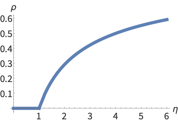
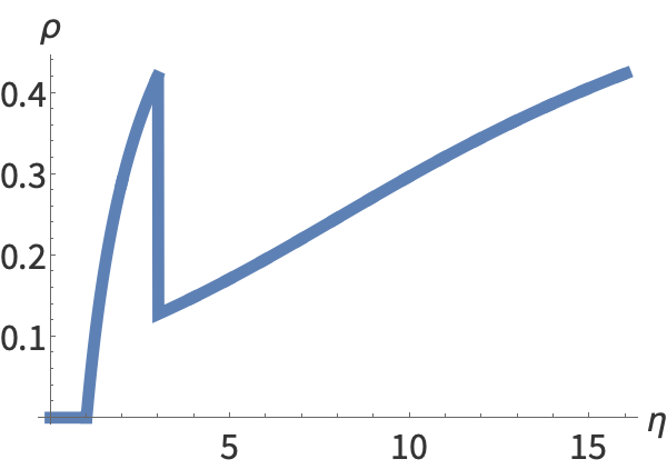
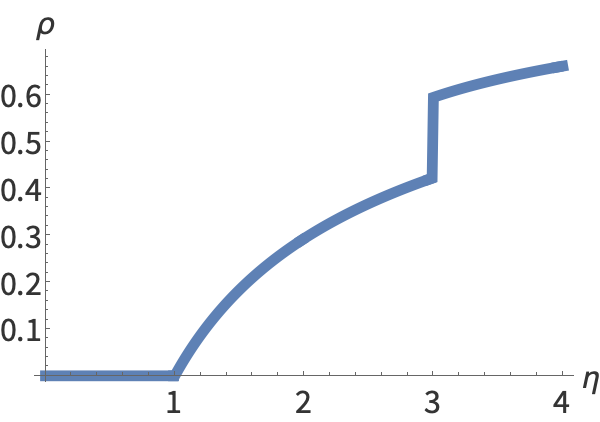
$\mathfrak{h}$

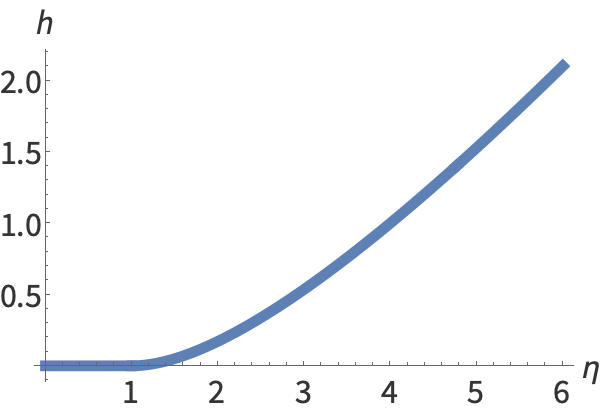
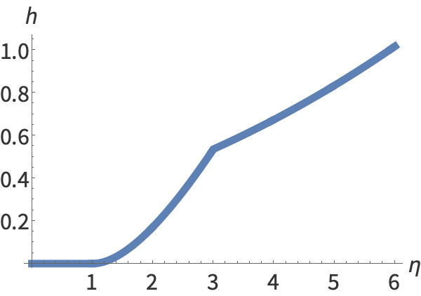
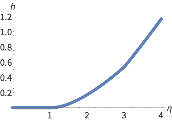
Figure 2. Limiting density and height function for three cases of piecewise linear $\boldsymbol{\xi}(\cdot)$.

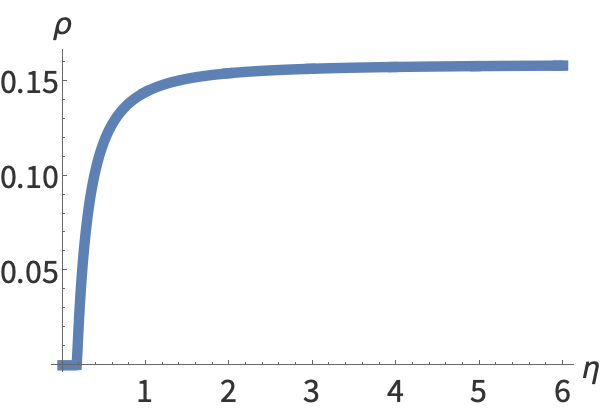
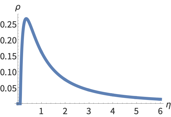
Figure 3. Two more examples of limiting density, for $\boldsymbol{\xi}(x)=x+\frac{1}{10}$ (left) and $\boldsymbol{\xi}(x)=x^{2}+\frac{1}{10}$ (right) on the interval $[0,6]$. These numerical computations suggest that many particles run off to infinity — a positive proportion (left) or all of them (right). Note that in both cases the speed function $\boldsymbol{\xi}(\cdot)$ is unbounded.

Theorem 1.13 (Limit shape).

Fix arbitrary $\tau,\eta>0$. If the limiting speed function $\boldsymbol{\xi}(\cdot)$ is piecewise continuously differentiable on $[0,\eta]$, then in the regime (1.7) we have the convergence $L^{-1}h(\tau L,\lfloor\eta L\rfloor)\to\mathfrak{h}(\tau,\eta)$ in probability as $L\to+\infty$. Here $h$ is the random height function of our PushTASEP, and $\mathfrak{h}$ is defined by (1.13).

Theorem 1.13 follows from the fluctuation result (Theorem 1.14) which is formulated next.

1.6. Asymptotic fluctuations

Using the notation of Section 1.5, define for $0<\tau<\tau_{e}(\eta)$:

$$\mathfrak{d}=\mathfrak{d}(\tau,\eta):=\left(\int_{0}^{\eta}\frac{\mathfrak{z}^{2}(\tau,\eta)\boldsymbol{\xi}(y)}{\left(\boldsymbol{\xi}(y)-\mathfrak{z}(\tau,\eta)\right)^{3}}\,dy\right)^{\frac{1}{3}}>0.$$ (1.15)

Note that this quantity is also continuous in $\eta$ similarly to Remark 1.12.1. The following is the main asymptotic fluctuation result of the present paper:

Theorem 1.14.

Fix arbitrary $\eta>0$ and $\tau\in(0,\tau_{e}(\eta))$. If the limiting speed function $\boldsymbol{\xi}(\cdot)$ is piecewise continuously differentiable on $[0,\eta]$, then in the regime (1.7) we have the convergence

$$\lim_{L\to+\infty}\mathbb{P}\left(\frac{h(\tau L,\lfloor\eta L\rfloor)-L\mathfrak{h}(\tau,\eta)}{\mathfrak{d}(\tau,\eta)L^{1/3}}>-r\right)=F_{GUE}(r),\qquad r\in\mathbb{R},$$ (1.16)

where $F_{GUE}$ is the GUE Tracy–Widom distribution [TW94].

This result implies the law of large numbers (Theorem 1.13).

Using the determinantal structure of Theorem 1.6, it is possible to also obtain (under slightly more restrictive smoothness conditions on $\boldsymbol{\xi}(\cdot)$) multipoint asymptotic fluctuation results along space-like paths. These fluctuations are governed by the top line of the Airy₂ line ensemble [PS02]. We will not focus on this result as it is a standard (by now) extension of the single-point fluctuations of Theorem 1.14. The extension readily follows from the determinantal structure together with a double contour integral kernel. For example, see [FS03] or [BF08], [BFS08] for such computations for random tilings and TASEP-like particle systems, respectively.

Remark 1.15.

Theorem 1.14 means that the insertion of inhomogeneity does not affect the fluctuation behavior of the PushTASEP compared to the homogeneous case. On the other hand, the inhomogeneity we consider in this paper (1.7) is relatively “mild” — it varies only macroscopically but not microscopically, and also is bounded (so that behavior like Figure 3 is out of the present scope). It would be interesting to see if less regular inhomogeneity might lead to different fluctuation behavior, whether in the regime of Theorem 1.14, or around the “edge” $(\tau_{e}(\eta)L,\lfloor\eta L\rfloor)$. At this edge in the homogeneous case one sees fluctuations on the scale $L^{1/2}$ described by the largest eigenvalues of GUE random matrices, and this behavior should persist in the presence of “mild” inhomogeneity (1.7).

1.7. Outline

In Section 2 we describe the connection between the inhomogeneous PushTASEP and Schur processes, and establish Theorem 1.6. In Section 3 we perform asymptotic analysis and establish Theorems 1.13 and 1.14 on the limit shape and asymptotic fluctuations. In Appendix A we check that the limiting density $\uprho$ defined in Section 1.5 formally satisfies the hydrodynamic equation coming from the inhomogeneous PushTASEP.

1.8. Acknowledgments

I am grateful to Konstantin Matveev for an insightful remark on connections with RSK column insertion, and to Alexei Borodin, Alexey Bufetov, Patrik Ferrari, Alisa Knizel, and Axel Saenz for helpful discussions. I am also grateful to anonymous referees for valuable suggestions. The work was partially supported by the NSF grant DMS-1664617.

2. Schur processes and inhomogeneous PushTASEP

Here we present a self-contained proof of Theorem 1.6 which follows from results on Schur processes [OR03] and the two-dimensional stochastic particle dynamics introduced in [BF14].

2.1. Young diagrams

A partition is a nonincreasing integer sequence of the form $\lambda=(\lambda_{1}\geq\ldots\geq\lambda_{\ell(\lambda)}>0)$. The number of nonzero parts $\ell(\lambda)$ (which must be finite) is called the length of a partition. Partitions are represented by Young diagrams, such that $\lambda_{1},\lambda_{2},\ldots$ are lengths of the successive rows. The column lengths of a Young diagram are denoted by $\lambda_{1}^{\prime}\geq\lambda_{2}^{\prime}\geq\ldots$. They form the transposed Young diagram $\lambda^{\prime}$. See Figure 4 for an illustration.

Figure 4. A Young diagram $\lambda=(5,3,3,1,1,1)$ for which the transposed diagram is $\lambda^{\prime}=(6,3,3,1,1)$.

2.2. Schur functions

For each Young diagram $\lambda$, let $s_{\lambda}$ be the corresponding Schur symmetric function [Mac95, Ch. I.3]. Evaluated at $N$ variables $u_{1},\ldots,u_{N}$ (where $N\geq\ell(\lambda)$ is arbitrary), $s_{\lambda}$ becomes the symmetric polynomial

$$s_{\lambda}(u_{1},\ldots,u_{N})=\frac{\det[u_{i}^{\lambda_{j}+N-j}]_{i,j=1}^{N}}{\det[u_{i}^{N-j}]_{i,j=1}^{N}}.$$ (2.1)

If $N<\ell(\lambda)$, then $s_{\lambda}(u_{1},\ldots,u_{N})=0$ by definition. When all $u_{i}\geq 0$, the value $s_{\lambda}(u_{1},\ldots,u_{N})$ is also nonnegative.

Along with evaluating Schur functions at finitely many variables, we also need their Plancherel specializations defined as

$$s_{\lambda}(\mathrm{Pl}_{t}):=\lim_{K\to+\infty}s_{\lambda}\Big{(}\underbrace{\frac{t}{K},\ldots,\frac{t}{K}}_{\textnormal{$K$ times}}\Big{)},\qquad t\in\mathbb{R}_{\geq 0}.$$

This limit exists for every $\lambda$ (for example, see [Oko01, Section 2.1.4]). It can be expressed through the number of standard Young tableaux of shape $\lambda$, which is the same as the dimension of the corresponding irreducible representation of the symmetric group of order $\lambda_{1}+\lambda_{2}+\ldots$. The values $s_{\lambda}(\mathrm{Pl}_{t})$ are nonnegative for all $t\geq 0$. When $t=0$, we have $s_{\lambda}(\mathrm{Pl}_{0})=\mathbf{1}_{\lambda=\varnothing}$.

The Schur functions satisfy Cauchy summation identities. We will need the following version:

$$\sum_{\lambda}s_{\lambda}(u_{1},\ldots,u_{N})s_{\lambda}(\mathrm{Pl}_{t})=e^{t(u_{1}+\ldots+u_{N})},$$

where the sum runs over all Young diagrams. However, summands corresponding to $\ell(\lambda)>N$ vanish. There are also skew Schur symmetric functions $s_{\lambda/\mu}$ which may be defined as expansion coefficients as follows (since Schur polynomials form a linear basis in the space of symmetric polynomials in the corresponding variables, we expand $s_{\lambda}$ as a symmetric polynomial in $u_{N+1},\ldots,u_{N+M}$):

$$s_{\lambda}(u_{1},\ldots,u_{N+M})=\sum_{\mu}s_{\lambda/\mu}(u_{1},\ldots,u_{N})\,s_{\mu}(u_{N+1},\ldots,u_{N+M}).$$

The function $s_{\lambda/\mu}$ vanishes unless the Young diagram $\lambda$ contains $\mu$ (notation: $\lambda\supset\mu$). Skew Schur functions satisfy skew modifications of the Cauchy summation identity. They also admit Plancherel specializations, and, moreover, $s_{\lambda/\mu}(\mathrm{Pl}_{t})$ is expressed through the number of standard tableaux of the skew shape $\lambda/\mu$. We refer to, e.g., [Mac95, Ch I.5] for details.

2.3. Schur processes

Here we recall the definition (at appropriate level of generality) of Schur processes introduced in [OR03]. Let $\xi_{\bullet}$ be a speed function as in Section 1.2, and take a down-right path $\{(t_{i},N_{i})\}_{i=1}^{r}$ (Definition 1.3). A Schur process associated with these data is a probability distribution on sequences $(\lambda;\mu)$ of Young diagrams (see Figure 5 for an illustration)

$$\varnothing=\mu^{(1)}\subset\lambda^{(1)}\supset\mu^{(2)}\subset\lambda^{(2)}\supset\mu^{(3)}\subset\ldots\subset\lambda^{(r-1)}\supset\mu^{(r)}=\varnothing$$ (2.2)

with probability weights

$$\begin{split}\mathsf{SP}(\lambda;\mu)&=\frac{1}{Z_{\mathsf{SP}}}\prod_{i=1}^{r-1}s_{\lambda^{(i)}/\mu^{(i)}}(\mathrm{Pl}_{t_{i+1}-t_{i}})\prod_{j=1}^{r-1}s_{\lambda^{(j)}/\mu^{(j+1)}}(\xi_{(N_{j+1},N_{j}]})\\ &=\frac{1}{Z_{\mathsf{SP}}}\,s_{\lambda^{(1)}/\mu^{(1)}}(\mathrm{Pl}_{t_{2}-t_{1}})s_{\lambda^{(1)}/\mu^{(2)}}(\xi_{(N_{2},N_{1}]})s_{\lambda^{(2)}/\mu^{(2)}}(\mathrm{Pl}_{t_{3}-t_{2}})\ldots\\ &\hskip 150.0pt\times s_{\lambda^{(r-1)}/\mu^{(r-1)}}(\mathrm{Pl}_{t_{r}-t_{r-1}})s_{\lambda^{(r-1)}/\mu^{(r)}}(\xi_{(N_{r},N_{r-1}]}).\end{split}$$ (2.3)

Here $\xi_{(a,b]}$ for $a\leq b$ means the string $(\xi_{a+1},\ldots,\xi_{b})$. Note that some of the specializations above can be empty. The normalizing constant in (2.3) is

$$Z_{\mathsf{SP}}=\exp\biggl{\{}\sum_{i=2}^{r}t_{i}\bigl{(}\xi_{N_{i}+1}+\ldots+\xi_{N_{i-1}}\bigr{)}\biggr{\}},$$

which is computed using the skew Cauchy identity.

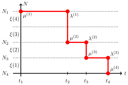
Figure 5. An illustration of the Schur process (2.3) corresponding to a down-right path with $r=4$. For convenience we take $t_{1}=N_{r}=0$ so that the corresponding Young diagrams are almost sure empty under the Schur process.

The marginal distribution of any $\lambda^{(i)}$ under the Schur process (2.3) is a Schur measure [Oko01] whose probability weights are

$$\mathsf{SM}(\lambda^{(i)})=e^{-t_{i+1}(\xi_{1}+\ldots+\xi_{N_{i}})}s_{\lambda^{(i)}}\bigl{(}\xi_{1},\xi_{2},\ldots,\xi_{N_{i}}\bigr{)}s_{\lambda^{(i)}}(\mathrm{Pl}_{t_{i+1}}).$$ (2.4)

2.4. Correlation kernel

As shown in [OR03, Theorem 1], the Schur process such as (2.3) can be interpreted as a determinantal random point process, and its correlation kernel is expressed as a double contour integral. To recall this result, consider the particle configuration

$$\Bigl{\{}\lambda^{(i)}_{j}-j\colon i=1,\ldots,r-1,\ j=1,2,\ldots\Bigr{\}}\subset\underbrace{\mathbb{Z}\times\ldots\times\mathbb{Z}}_{\textnormal{$r-1$ times}}$$ (2.5)

corresponding to a sequence (2.2) (where we sum over all the $\mu^{(j)}$’s). The configurations $\lambda^{(i)}_{j}-j$, $j\geq 1$, are infinite and are densely packed at $-\infty$ (i.e., we append each $\lambda^{(i)}$ by infinitely many zeroes). Then for any $m$ and any pairwise distinct locations $(l_{i},x_{i})$, $i=1,\ldots,m$, where $1\leq l_{i}\leq r-1$ and $x_{i}\in\mathbb{Z}$, we have

$$\begin{split}&\mathbb{P}\Bigl{(}\textnormal{there are points of the configuration \eqref{eq:particle_configuration_for_Schur_process} at each of the locations $(l_{i},x_{i})$}\Bigr{)}\\ &\hskip 280.0pt=\det\left[K_{\mathsf{SP}}(l_{i},x_{i};l_{j},x_{j})\right]_{i,j=1}^{m}.\end{split}$$

The kernel $K_{\mathsf{SP}}$ has the form

$$K_{\mathsf{SP}}(l,x;l^{\prime},y)=\frac{1}{(2\pi\mathbf{i})^{2}}\oint\oint\frac{dz\,dw}{z-w}\frac{w^{y}}{z^{x+1}}\frac{\Phi(l,z)}{\Phi(l^{\prime},w)},$$ (2.6)

where

$$\Phi(l,z)=e^{zt_{l+1}}\prod_{i=1}^{N_{l}}(1-z^{-1}\xi_{i}).$$

The integration contours in (2.6) are positively oriented simple closed curves around $0$, the contour $w$ in addition encircles $\{\xi_{x}\}_{x\in\mathbb{Z}_{\geq 1}}$, and on these contours $|z|>|w|$ for $l\leq l^{\prime}$ and $|z|<|w|$ for $l>l^{\prime}$.

2.5. Coupling PushTASEP and Schur processes

Fix a speed function $\xi_{\bullet}$ as above. We will consider (half continuous Schur) random fields of Young diagrams

$$\{\lambda^{(t,N)}\colon t\in\mathbb{R}_{\geq 0},N\in\mathbb{Z}_{\geq 1}\}$$

satisfying the following properties:

1. (Schur field property) For any down-right path $\{(t_{i},N_{i})\}_{i=1}^{r}$, the joint distribution of the Young diagrams $\lambda^{(i)}=\lambda^{(t_{i+1},N_{i})}$ is described by the Schur process corresponding to this down-right path. Note that this almost surely enforces the boundary conditions $\lambda^{(0,N)}=\lambda^{(t,0)}\equiv\varnothing$, and also forces each diagram $\lambda^{(t,N)}$ to have at most $N$ parts.

2. (PushTASEP coupling property) The collection of random variables

   $$\{N-\lambda_{1}^{\prime(t,N)}\colon t\in\mathbb{R}_{\geq 0},N\in\mathbb{Z}_{\geq 1}\}$$ (2.7)

   (where $\lambda_{1}^{\prime(t,N)}$ is the length of the first column of $\lambda^{(t,N)}$) has the same distribution as the values of the height function

   $$\{h(t,N)\colon t\in\mathbb{R}_{\geq 0},N\in\mathbb{Z}_{\geq 1}\}$$ (2.8)

   in the inhomogeneous PushTASEP having the speed function $\xi_{\bullet}$ and started from the empty initial configuration.

The first property states that a field couples together Schur processes with different parameters in a particular way, and the second property requires a field to possess additional structure relating it to the PushTASEP. The random field point of view was recently useful in [BBW18], [BM18], [BP19], [BMP19] in discovering and studying particle systems powered by generalizations of Schur processes.

The above two properties do not determine a field uniquely. In fact, there exist several constructions of fields satisfying these properties. They lead to different joint distributions of all the diagrams $\{\lambda^{(t,N)}\}$. However, due to the Schur field property, along down-right paths the joint distributions of diagrams are the same.

The oldest known such construction is based on the column RSK insertion. Connections between RSK, random Young diagrams, and stochastic particle systems can be traced [VK86], see also [O’C03b], [O’C03a]. Another field coupling Schur processes and the PushTASEP was suggested in [BF14] based on an idea [DF90] of stitching together Markov processes connected by a Markov projection operator. A unified treatment of these two approaches was performed in [BP16], see also [OP13]. A variation of the field of [BF14] based on the Yang-Baxter equation was suggested recently in [BP19] (for Schur processes, as well as for their certain two-parameter generalizations), and further extended in [BMP19]. Since either of these approaches suffices for our purposes, let us outline the simplest one from [BF14].

Fix $K\geq 1$, and consider the restriction of the field to the first $K$ horizontal levels. Interpret $t$ as continuous time, and the integers $\{\lambda^{(t,N)}_{i}\colon 1\leq N\leq K,1\leq i\leq N\}$ as a two-dimensional time-dependent array. We will describe a Markov evolution of this array. Throughout the evolution, the integers will almost surely satisfy the interlacing constraints $\lambda^{(t,i)}_{j+1}\leq\lambda^{(t,i-1)}_{j}\leq\lambda^{(t,i)}_{j}$ for all $i,j$ and at all times $t$. These interlacing constraints are visualized in Figure 6.

Figure 6. Interlacing array.

The array evolves as follows. Each of the integers at each level $1\leq N\leq K$ has an independent exponential clock with rate $\xi_{N}$. When the clock of $\lambda^{(t,N)}_{j}$ rings (almost surely, at most one clock can ring at a given time moment since the number of clocks is finite), its value is generically incremented by one. In addition, the following mechanisms are at play to preserve interlacing in the course of the evolution:

• (blocking) If $\lambda^{(t,N)}_{j}=\lambda^{(t,N-1)}_{j-1}$ before the increment of $\lambda^{(t,N)}_{j}$, then this increment is suppressed;

• (mandatory pushing) If $\lambda^{(t,N)}_{j}=\lambda^{(t,N+1)}_{j}=\ldots=\lambda^{(t,N+m)}_{j}$ for some $m\geq 1$ before the increment of $\lambda^{(t,N)}_{j}$, then along with adding one to $\lambda^{(t,N)}_{j}$, we also increment by one each of $\lambda^{(t,N+1)}_{j},\ldots,\lambda^{(t,N+m)}_{j}$.

Thus described Markov processes are compatible for various $K$, and so they define a random field $\lambda^{(t,N)}$, $t\in\mathbb{R}_{\geq 0}$, $N\in\mathbb{Z}_{\geq 1}$. From [BF14] (see also, e.g., [BP16, Section 2] for a relatively brief outline of the general formalism) it follows that the collection of random Young diagrams $\{\lambda^{(t,N)}\}$ satisfies the Schur field property, i.e., its distributions along down-right paths are given by Schur processes.

Remark 2.1.

Note that the interlacing inequalities in Figure 6 are non-strict, while after the shifting as in (2.5) some of these inequalities between consecutive levels become strict.

Proof of the PushTASEP coupling property..

Let us now prove that the just constructed collection $\{\lambda^{(t,N)}\}$ of Young diagrams satisfies the PushTASEP coupling property. Observe that $N-\lambda_{1}^{\prime}(t,N)$ is the number of zeroes in the $N$-th row in the array in Figure 6. Due to interlacing, for each fixed $t$ we can interpret $\tilde{h}(t,N):=N-\lambda_{1}^{\prime}(t,N)$ as the height function of a particle configuration $\tilde{\mathsf{x}}(t)=\{\tilde{\mathsf{x}}_{i}(t)\}_{i\geq 1}$ in $\mathbb{Z}_{\geq 1}$, with at most one particle per site. The initial condition is $\tilde{\mathsf{x}}_{i}(0)=i$, $i\geq 1$. That is, we can determine $\tilde{\mathsf{x}}$ from $\tilde{h}$ using (1.2).

The time evolution of the particle configuration $\tilde{\mathsf{x}}(t)$ is recovered from the field $\lambda^{(t,N)}$. First, observe that any change in $\tilde{\mathsf{x}}$ can come only from the exponential clocks ringing at the rightmost zero elements of the interlacing array. There are two cases. If $\tilde{h}(t,N)=\tilde{h}(t,N-1)$, then the rightmost clock at zero on level $N$ corresponds to a blocked increment, which agrees with the fact that $\tilde{\mathsf{x}}$ has no particle at location $N$. If, on the other hand, $\tilde{h}(t,N)=\tilde{h}(t,N-1)+1$, then there is a particle in $\tilde{\mathsf{x}}$ at $N$ which can jump to the right by one. This happens at rate $\xi_{N}$. If this particle at $N$ jumps and, moreover, $\tilde{h}(t,N+1)=\tilde{h}(t,N)+1$, then the particle at $N+1$ which is also present in $\tilde{\mathsf{x}}$ is pushed by one to the right, and so on. See Figure 7 for illustration.

Figure 7. Left: in the interlacing array the framed zero is blocked and cannot increase. This corresponds to no particle in $\tilde{\mathsf{x}}(t)$ at $N$. Right: the circled zero at level $N$ decides to increase at rate $\xi_{N}$, and forces the circled zero at level $N+1$ to increase, too. In $\tilde{\mathsf{x}}(t)$ this corresponds to a jump of the particle at $N$ which then pushes a particle at $N+1$.

We see that the Markov process $\tilde{\mathsf{x}}(t)$ coincides with the PushTASEP in inhomogeneous space $\mathsf{x}(t)$ introduced in Section 1.2. ∎

Remark 2.2.

The field $\lambda^{(t,N)}$ from [BF14] described above has another Markov projection to a particle system in $\mathbb{Z}$ which coincides with the PushTASEP with particle-dependent inhomogeneity. Namely, start the PushTASEP from the step initial configuration $\mathsf{x}_{i}(t)=i$, $i\geq 1$, and let the particle $\mathsf{x}_{i}$ have jump rate $\xi_{i}$. The space is assumed homogeneous, so now variable jump rates are attached to particles. Then the joint distribution of the random variables $\{\mathsf{x}_{i}(t)\}$ for all $t\geq 0$, $i\geq 1$, coincides with the joint distribution of $\{\lambda^{(t,i)}_{1}+i\}$. In particular, each $\mathsf{x}_{N}(t)$ has the same distribution as $\lambda_{1}+N$ under the Schur measure $\propto s_{\lambda}(\xi_{1},\ldots,\xi_{N})s_{\lambda}(\mathrm{Pl}_{t})$ (this is the same Schur measure as in (2.4)). Asymptotic behavior of PushTASEP with particle-dependent jump rates was studied in [BG13] by means of Rákos–Schütz type determinantal formulas [RS05], [BF08].

A third Markov projection of the field $\lambda^{(t,N)}$ onto $\{\lambda^{(t,N)}_{N}-N\}_{N\geq 1}$ recovers TASEP on $\mathbb{Z}$ with particle-dependent speeds. We refer to [BF14] for details on these other two Markov projections.

2.6. From coupling to determinantal structure

For any random field $\lambda^{(t,N)}$ satisfying the Schur field property, the determinantal structure result of [OR03] recalled in Section 2.4 can be restated as follows:

Theorem 2.3.

For any $m\in\mathbb{Z}_{\geq 1}$ and any collection of pairwise distinct locations $\{(t_{i},N_{i},x_{i})\}_{i=1}^{m}\subset\mathbb{R}\times\mathbb{Z}\times\mathbb{Z}$ such that $N_{1}\geq\ldots\geq N_{m}\geq 0$ and $0\leq t_{1}\leq\ldots\leq t_{m}$, we have

$$\mathbb{P}\Bigl{(}\textnormal{for all $i=1,\ldots,m$, the configuration $\{\lambda^{(t_{i},N_{i})}_{j}-j\}_{j\geq 1}$ contains a particle at $x_{i}$}\Bigr{)}\\ =\det\left[K_{\mathsf{F}}(t_{p},N_{p},x_{p};t_{q},N_{q},x_{q})\right]_{p,q=1}^{m},$$

where

$$K_{\mathsf{F}}(t,N,x;s,M,y):=\frac{1}{(2\pi\mathbf{i})^{2}}\oint\oint\frac{dz\,dw}{z-w}\frac{w^{y+M}}{z^{x+N+1}}\exp\bigl{\{}tz-sw\bigr{\}}\frac{\prod_{a=1}^{N}\bigl{(}z-\xi_{a}\bigr{)}}{\prod_{b=1}^{M}\bigl{(}w-\xi_{b}\bigr{)}}.$$ (2.9)

The integration contours are positively oriented simple closed curves around $0$, the $w$ contour additionally encircles $\{\xi_{x}\}_{x\in\mathbb{Z}_{\geq 1}}$, and the contours satisfy $|z|>|w|$ for $t\leq s$ and $|z|<|w|$ for $t>s$.

In particular, this theorem applies to the field from [BF14] recalled in Section 2.5 whose first columns are related to the PushTASEP as in (2.7)–(2.8).

2.7. Kernel for column lengths

Let us restate Theorem 2.3 in terms of column lengths so that we can apply it to PushTASEP.

Proposition 2.4.

Let $\lambda$ be a Young diagram. The complement in $\mathbb{Z}$ of the point configuration $\{\lambda_{j}-j\}_{j\geq 1}$ is the point configuration $\{-\lambda_{i}^{\prime}+i-1\}_{i\geq 1}$. The former configuration is densely packed at $-\infty$, and the latter one at $+\infty$.

Proof.

A straightforward verification, see Figure 8. ∎

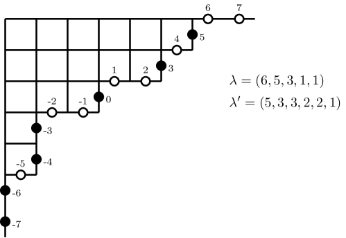
Figure 8. Configuration $\{\lambda_{j}-j\}$ and its complement configuration $\{-\lambda_{i}^{\prime}+i-1\}$, both placed at the boundary of the Young diagram $\lambda$.

The correlation kernel for the complement configuration is given by $K:=\mathbf{1}-K_{\mathsf{F}}$, where $\mathbf{1}$ is the identity operator whose kernel is the delta function. This follows from an observation of S. Kerov based on the inclusion-exclusion principle see [BOO00, Appendix A.3]. This leads to:

Corollary 2.5.

For $\{(t_{i},N_{i},x_{i})\}_{i=1}^{m}\subset\mathbb{R}\times\mathbb{Z}\times\mathbb{Z}$ as in Theorem 2.3, we have

$$\mathbb{P}\Bigl{(}\textnormal{$x_{i}\in\{-\lambda^{\prime(t_{i},N_{i})}_{j}+j-1\}_{j\geq 1}$ for all $i=1,\ldots,m$}\Bigr{)}=\det\left[K(t_{p},N_{p},x_{p};t_{q},N_{q},x_{q})\right]_{p,q=1}^{m},$$

where the kernel $K(t,N,x;s,M,y):=\mathbf{1}_{t=s}\mathbf{1}_{N=M}\mathbf{1}_{x=y}-K_{\mathsf{F}}(t,N,x;s,M,y)$ is given by formula (1.4) in the Introduction.

Proof of Theorem 1.6.

This theorem now readily follows from Corollary 2.5 and the PushTASEP coupling property of Section 2.5. ∎

2.8. Fredholm determinants

Let us now utilize Section 2.5 and Corollary 2.5 to write down observables of the PushTASEP in inhomogeneous space in terms of Fredholm determinants.

First, recall Fredholm determinants on an abstract discrete space $\mathfrak{X}$. Let $K(x,y)$, $x,y\in\mathfrak{X}$ be a kernel on this space. We say that the Fredholm determinant of $\mathbf{1}+zK$, $z\in\mathbb{C}$, is an infinite series

$$\det(1+zK)_{\mathfrak{X}}=1+\sum_{r=1}^{\infty}\frac{z^{r}}{r!}\sum_{i_{1}\in\mathfrak{X}}\ldots\sum_{i_{r}\in\mathfrak{X}}\det\left[K(i_{p},i_{q})\right]_{p,q=1}^{r}.$$ (2.10)

One may view (2.10) as a formal series, but in our setting this series will converge numerically. Details on Fredholm determinants may be found in [Sim05] or [Bor10].

Fix a down-right path $\mathfrak{p}=\{(t_{i},N_{i})\}_{i=1}^{r}$ and consider the space

$$\mathcal{X}=\mathcal{X}_{1}\sqcup\ldots\sqcup\mathcal{X}_{r},\qquad\mathcal{X}_{i}=\mathbb{Z}.$$

For $y\in\mathcal{X}_{i}$ set $t(y)=t_{i}$, $N(y)=N_{i}$. View $\{-\lambda_{j}^{\prime(t_{i},N_{i})}+j-1\}_{j\geq 1,\;i=1,\ldots,r}$ as a determinantal process $\mathfrak{L}_{\mathfrak{p}}$ on $\mathcal{X}$ with kernel $K$ (1.4) in the sense of Corollary 2.5.

Fix an arbitrary $r$-tuple $\vec{y}=(y_{1},\ldots,y_{r})\in\mathbb{Z}^{r}$. We can interpret

$$\mathbb{P}\Bigl{(}h(t_{i},N_{i})>N_{i}-y_{i},\ i=1,\ldots,r\Bigr{)}=\mathbb{P}\Bigl{(}-\lambda_{1}^{\prime(t_{i},N_{i})}>-y_{i},\ i=1,\ldots,r\Bigr{)}$$

as the probability of the event that there are no points in the random point configuration $\mathfrak{L}_{\mathfrak{p}}$ in the subset $\mathcal{X}_{\vec{y}}:=\bigsqcup_{i=1}^{r}\left\{\ldots,-y_{i}-2,-y_{i}-1,-y_{i}\right\}$ of $\mathcal{X}$. This probability can be written (e.g., see [Sos00]) as the Fredholm determinant

$$\det(1-\chi_{\vec{y}}K\chi_{\vec{y}})_{\mathcal{X}},$$ (2.11)

where $\chi_{\vec{y}}(x)=\mathbf{1}_{x\leq-y_{i}}$ for $x\in\mathcal{X}_{i}$ is the indicator of $\mathcal{X}_{\vec{y}}\subset\mathcal{X}$ viewed as a projection operator acting on functions. In particular, for $r=1$ this implies Corollary 1.7 from the Introduction.

Remark 2.6.

One can check that the sums in the Fredholm determinant (2.11) (as well as in (1.6) in the Introduction) are actually finite due to vanishing of $K$ far to the left.

3. Asymptotic analysis

In this section we study asymptotic fluctuations of the random height function of the inhomogeneous PushTASEP at a single space-time point, and prove Theorems 1.13 and 1.14. We also establish more general results on approximating the kernel $K$ (1.4) by the Airy kernel under weaker assumptions on $\boldsymbol{\xi}(\cdot)$.

3.1. Rewriting the kernel

Let us rewrite $K$ given by (1.4) to make the integration contours suitable for asymptotic analysis via steepest descent method.

Proposition 3.1.

Let $x^{\prime}<0$ and $t^{\prime}>0$. Then

$$\begin{split}&K(t,N,x;t^{\prime},N^{\prime},x^{\prime})=\mathbf{1}_{t=t^{\prime}}\mathbf{1}_{N=N^{\prime}}\mathbf{1}_{x=x^{\prime}}-\frac{\mathbf{1}_{t\leq t^{\prime}}}{2\pi\mathbf{i}}\oint\frac{e^{(t-t^{\prime})z}dz}{z^{x-x^{\prime}+N-N^{\prime}+1}}\prod_{b=N^{\prime}+1}^{N}(z-\xi_{b})\\ &\hskip 120.0pt-\frac{1}{(2\pi\mathbf{i})^{2}}\oint dz\int dw\,\frac{e^{tz-t^{\prime}w}}{z-w}\frac{w^{x^{\prime}+N^{\prime}}}{z^{x+N+1}}\frac{\prod_{a=1}^{N}(z-\xi_{a})}{\prod_{b=1}^{N^{\prime}}(w-\xi_{b})}.\end{split}$$ (3.1)

Here the $z$ contour in both integrals is a positively oriented circle around $0$ (of arbitrary positive radius, say, $\delta$), and the $w$ contour in the double integral is the vertical line $-2\delta+\mathbf{i}\mathbb{R}$ traversed downwards and located to the left of the $z$ contour.

Proof.

We start from formula (1.4) for the kernel. For $t\leq t^{\prime}$ (thus necessarily $N\geq N^{\prime}$ because we consider correlations only along down-right paths, cf. Definition 1.3) the $z$ contour encircles the $w$ contour. Note that the integrand does not have poles in $z$ at the $\xi_{a}$’s. Thus, exchanging for $t\leq t^{\prime}$ the $z$ contour with the $w$ contour at a cost of an additional residue, we see that the new contours in the double integral in (1.4) can be taken as follows:

• the $z$ contour is a small positive circle around $0$;

• the $w$ contour is a large positive circle around $0$ and $\{\xi_{a}\}_{a\geq 1}$.

The additional residue arising for $t\geq t^{\prime}$ is equal to the integral of the residue at $z=w$ of the integrand over the single $w$ contour. Because $t\leq t^{\prime}$ and $N\geq N^{\prime}$, this residue does not have poles at the $\xi_{a}$’s, and so the integration can be performed over a small contour around $0$. Renaming $w$ to $z$ we arrive at the single integral in (3.1).

Finally, in the double integral the $w$ integration contour can be replaced by a vertical line because:

• the exponent $e^{-t^{\prime}w}$ ensures rapid decay of the absolute value of the integrand sufficiently far in the right half plane;

• the polynomial factors $\frac{w^{x^{\prime}+N^{\prime}}}{z-w}\prod_{b=1}^{N^{\prime}}(w-\xi_{b})^{-1}$ for $x^{\prime}<0$ ensure at least quadratic decay of the absolute value of the integrand for sufficiently large $|\mathop{\mathrm{Im}}w|$.

This completes the proof. ∎

Remark 3.2.

The assumption $x^{\prime}<0$ made in Proposition 3.1 agrees with the fact that we are looking at the leftmost points in the determinantal point process $\mathfrak{L}_{\mathfrak{p}}$ (Theorem 1.6), and these leftmost points almost surely belong to $\mathbb{Z}_{\leq 0}$. At the level of the PushTASEP this corresponds to $h(t,N)\leq N$. The event $h(t,N)=N$ (i.e., for which it would be $x^{\prime}=0$) can be excluded, too, since it corresponds to no particles $\leq N$ jumping till time $t$. Since $t$ goes to infinity, this is almost surely impossible. We thus assume that $x^{\prime}<0$ throughout the text.

3.2. Critical points and estimation on contours

Rewrite the integrand in the double contour integral in (3.1) as

$$\frac{(-1)^{h+h^{\prime}+N+N^{\prime}+1}}{z(z-w)}\exp\bigl{\{}S_{L}(z;t,N,h)-S_{L}(w;t^{\prime},N^{\prime},h^{\prime})\bigr{\}},$$ (3.2)

where $h:=x+N$, $h^{\prime}:=x^{\prime}+N^{\prime}$, and the function $S_{L}$ has the form

$$S_{L}(z;t,N,h):=tz-h\log(-z)+\sum_{a=1}^{N}\log\left(\xi_{a}-z\right).$$ (3.3)

The signs inside logarithms are inserted for future convenience. The branches of the logarithms are assumed standard, i.e., they have cuts along the negative real axis.

We apply the steepest descent approach (as outlined in, e.g., [Oko02, Section 3], in a stochastic probabilistic setting) to analyze the asymptotic behavior of the leftmost points of the determinantal process $\mathfrak{L}_{\mathfrak{p}}$. To this end, we consider double critical points of $S_{L}$ which satisfy the following system of equations:

$$t =\sum_{a=1}^{N}\frac{\xi_{a}}{\left(z-\xi_{a}\right)^{2}},$$ (3.4)

$$h =\sum_{a=1}^{N}\frac{z^{2}}{\left(z-\xi_{a}\right)^{2}}.$$ (3.5)

Definition 3.3.

By analogy with (1.11), denote $t_{e}(N):=\sum\limits_{a=1}^{N}\xi_{a}^{-1}$.

In the rest of this subsection we assume that $N\geq 1$ and $0<t<t_{e}(N)$ are fixed.

Lemma 3.4.

Equation (3.4) has a unique solution in real negative $z$.

Proof.

Follows by monotonicity similarly to Lemma 1.10. ∎

Denote the solution afforded by Lemma 3.4 by $\mathfrak{z}_{L}=\mathfrak{z}_{L}(t,N)$. Also denote by $\mathfrak{h}_{L}=\mathfrak{h}_{L}(t,N)$ the result of substitution of $\mathfrak{z}_{L}(t,N)$ into the right-hand side of (3.5).

Lemma 3.5.

The function $z\mapsto S_{L}(z;t,N,\mathfrak{h}_{L}(t,N))$ has a double critical point at $\mathfrak{z}_{L}(t,N)$ which is its only critical point on the negative real half-line. All other critical points (of any order) of this function are real and positive.

Proof.

The fact that $\mathfrak{z}_{L}(t,N)$ is a double critical point of $S_{L}(\cdot;t,N,\mathfrak{h}_{L}(t,N))$ follows from the above definitions. It remains to check that all other critical points of $S_{L}$ are real and positive. Let $0<b_{1}<\ldots<b_{k}$ be all of the distinct values of $\xi_{1},\ldots,\xi_{N}$. Then equation $S_{L}^{\prime}(z)=0$, that is,

$$\frac{h}{z}=t+\sum_{a=1}^{N}\frac{1}{z-\xi_{a}}$$ (3.6)

is equivalent to a polynomial equation of degree $k+1$ with real coefficients. The right-hand side of (3.6) takes all values from $-\infty$ to $+\infty$ on each of the $k-1$ intervals of the form $(b_{i},b_{i+1})$. Therefore, (3.6) has at least $k-1$ positive real roots. Since $\mathfrak{z}_{L}$ is a double root when $h=\mathfrak{h}_{L}$, we have described at least $k+1$ real roots to the equation $S_{L}^{\prime}(z)=0$, i.e., all of its roots. This completes the proof. ∎

Keeping $t,N$ fixed, plug $h=\mathfrak{h}_{L}(t,N)$ into $S_{L}$, and using (3.4)–(3.5) rewrite the result in terms of $\mathfrak{z}_{L}$:

$$S_{L}(z;t,N,\mathfrak{h}_{L}(t,N))=\sum_{a=1}^{N}\left[\frac{z\xi_{a}}{(\mathfrak{z}_{L}-\xi_{a})^{2}}-\frac{\mathfrak{z}_{L}^{2}\log(-z)}{(\mathfrak{z}_{L}-\xi_{a})^{2}}+\log(\xi_{a}-z)\right].$$

Denote the expression inside the sum by $R(z;\xi_{a})$.

Lemma 3.6.

On the circle through $\mathfrak{z}_{L}$ centered at the origin, $\mathop{\mathrm{Re}}S_{L}(z;t,N,\mathfrak{h}_{L}(t,N))$ viewed as a function of $z$ attains its maximum at $z=\mathfrak{z}_{L}$.

Proof.

For $z=\mathfrak{z}_{L}e^{\mathbf{i}\varphi}$, we have

$$\frac{\partial}{\partial\varphi}\mathop{\mathrm{Re}}R(\mathfrak{z}_{L}e^{\mathbf{i}\varphi};\xi)=\frac{2\xi^{2}\mathfrak{z}_{L}^{2}(\cos\varphi-1)\sin\varphi}{(\mathfrak{z}_{L}-\xi)^{2}\left(\xi^{2}+\mathfrak{z}_{L}^{2}-2\mathfrak{z}_{L}\xi\cos\varphi\right)}\leq 0$$

for $\varphi\in[0,\pi]$ (by symmetry, it suffices to consider only the upper half plane), and this derivative is equal to zero only for $\varphi=0$. This implies the claim. ∎

Lemma 3.7.

On the vertical line $\mathfrak{z}_{L}+\mathbf{i}\mathbb{R}$ through $\mathfrak{z}_{L}$, $\mathop{\mathrm{Re}}S_{L}(w;t,N,\mathfrak{h}_{L}(t,N))$ viewed as a function of $w$ attains its minimum at $w=\mathfrak{z}_{L}$.

Proof.

For $w=\mathfrak{z}_{L}+\mathbf{i}r$, $r>0$, we have

$$\frac{\partial}{\partial r}\mathop{\mathrm{Re}}R(\mathfrak{z}_{L}+\mathbf{i}r;\xi)=\frac{r^{3}\left(\xi^{2}+\mathfrak{z}_{L}^{2}-2\mathfrak{z}_{L}\xi-\mathfrak{z}_{L}\right)-r\mathfrak{z}_{L}(1-\mathfrak{z}_{L})(\xi-\mathfrak{z}_{L})^{2}}{\left(r^{2}+\mathfrak{z}_{L}^{2}\right)(\mathfrak{z}_{L}-\xi)^{2}\left(\xi^{2}+r^{2}+\mathfrak{z}_{L}^{2}-2\mathfrak{z}_{L}\xi\right)}>0$$

(recall that $\mathfrak{z}_{L}<0$). This implies the claim. ∎

We need one more statement on derivatives of the real part at the double critical point:

Lemma 3.8.

Along the $w$ and $z$ contours in Lemmas 3.6 and 3.7 the first three derivatives of $\mathop{\mathrm{Re}}S_{L}$ vanish at $\mathfrak{z}_{L}$, while the fourth derivative is nonzero.

Proof.

One readily checks that $(\frac{\partial}{\partial\varphi})^{k}\mathop{\mathrm{Re}}R(\mathfrak{z}_{L}e^{\mathbf{i}\varphi};\xi)\,\big{|}_{\varphi=0}=0$ for $k=1,2,3$, and it is equal to $-\frac{6\mathfrak{z}_{L}^{2}\xi^{2}}{(\mathfrak{z}_{L}-\xi)^{4}}<0$ for $k=4$. The case of the $w$ contour is analogous with a strictly positive fourth derivative in $r$ of $\mathop{\mathrm{Re}}R(\mathfrak{z}_{L}+\mathbf{i}r;\xi)$. ∎

Let us now deform the integration contours in the double contour integral in (3.1) so that they are as in Lemmas 3.6 and 3.7 (but locally do not intersect at $\mathfrak{z}_{L}$). We can perform this deformation without picking any residues in particular because the integrand is regular in $z$ at all the $\xi_{a}$’s. Lemmas 3.6 and 3.7 then imply that the asymptotic behavior of the integral for large $L$ is determined by the contribution coming from the neighborhood of the double critical point $\mathfrak{z}_{L}$. In Section 3.4 we make precise estimates.

3.3. Airy kernel

Before we proceed, let us recall the Airy kernel [TW93], [TW94]

$$\begin{split}\mathsf{A}(x;y):=\frac{1}{(2\pi\mathbf{i})^{2}}\iint\frac{e^{u^{3}/3-v^{3}/3-xu+yv}du\,dv}{u-v}=\frac{\mathsf{Ai}(x)\mathsf{Ai}^{\prime}(y)-\mathsf{Ai}^{\prime}(x)\mathsf{Ai}(y)}{x-y},\end{split}$$ (3.7)

where $x,y\in\mathbb{R}$ (the second expression is extended to $x=y$ by continuity). In the contour integral expression, the $v$ integration contour goes from $e^{-\mathbf{i}\frac{2\pi}{3}}\infty$ through $0$ to $e^{\mathbf{i}\frac{2\pi}{3}}\infty$, and the $u$ contour goes from $e^{-\mathbf{i}\frac{\pi}{3}}\infty$ through $0$ to $e^{\mathbf{i}\frac{\pi}{3}}\infty$, and the integration contours do not intersect.

The GUE Tracy–Widom distribution function is the following Fredholm determinant of (3.7):

$$F_{GUE}(r)=\det\left(\mathbf{1}-\mathsf{A}\right)_{(r,+\infty)},\qquad r\in\mathbb{R}.$$ (3.8)

Its expansion is defined analogously to (2.10) but with sums replaced with integrals over $(r,+\infty)$.

3.4. Approximation and convergence

Our first estimate is a standard approximation of the kernel $K(t,N,x;t,N,x^{\prime})$ by the Airy kernel $\mathsf{A}$ (3.7) when both $x,x^{\prime}$ are close to $\mathfrak{h}_{L}(t,N)-N$. Denote

$$\mathfrak{d}_{L}=\mathfrak{d}_{L}(t,N):=\biggl{(}\frac{1}{L}\sum_{a=1}^{N}\frac{\mathfrak{z}_{L}^{2}(t,N)\xi_{a}}{\left(\xi_{a}-\mathfrak{z}_{L}(t,N)\right)^{3}}\biggr{)}^{1/3}>0.$$ (3.9)

In this subsection we assume that $t=t(L)$ and $N=N(L)$ depend on $L$ such that for all sufficiently large $L$:

• $0<t<t_{e}(N)-cL$ for some $c>0$;

• for some $m,M>0$ we have $m<\frac{t(L)}{L}<M$ and $m<\frac{N(L)}{L}<M$.

Lemma 3.9.

Under our assumptions on $(t(L),N(L))$, as $L\to+\infty$ we have

$$K(t,N,x;t,N,x^{\prime})=\bigl{(}-\mathfrak{z}_{L}(t,N)\bigr{)}^{(\mathsf{h}^{\prime}-\mathsf{h})L^{1/3}}\frac{L^{-1/3}}{\mathfrak{d}_{L}(t,N)}\mathsf{A}\biggl{(}-\frac{\mathsf{h}}{\mathfrak{d}_{L}(t,N)},-\frac{\mathsf{h}^{\prime}}{\mathfrak{d}_{L}(t,N)}\biggl{)}\bigl{(}1+O(L^{-1/3})\bigr{)},$$ (3.10)

where $x=\mathfrak{h}_{L}(t,N)-N+\mathsf{h}L^{1/3}$, $x^{\prime}=\mathfrak{h}_{L}(t,N)-N+\mathsf{h}^{\prime}L^{1/3}$, $\mathsf{h},\mathsf{h}^{\prime}\in\mathbb{R}$.

Proof.

When $(t,N)=(t^{\prime},N^{\prime})$, the indicator and the single contour integral in (3.1) cancel out, and so we have

$$\begin{split}K(t,N,x;t,N,x^{\prime})&=-\frac{1}{(2\pi\mathbf{i})^{2}}\oint dz\int dw\,\frac{e^{t(z-w)}}{z(z-w)}\frac{(-w)^{x+N}}{(-z)^{x+N}}\prod_{a=1}^{N}\frac{\xi_{a}-z}{\xi_{a}-w}\\ &=-\frac{1}{(2\pi\mathbf{i})^{2}}\oint dz\int dw\,\frac{e^{S_{L}(z;t,N,h)-S_{L}(w;t,N,h^{\prime})}}{z(z-w)},\end{split}$$ (3.11)

where $h=x+N$, $h^{\prime}=x^{\prime}+N$. Let the $z$ and $w$ integration contours pass near $\mathfrak{z}_{L}$ (without intersecting each other) and be as in Lemmas 3.6 and 3.7. We have

$$S_{L}(z;t,N,h)-S_{L}(w;t,N,h^{\prime})\\ =(\mathfrak{h}_{L}-h)\log(-z)+(h^{\prime}-\mathfrak{h}_{L})\log(-w)+S_{L}(z;t,N,\mathfrak{h}_{L})-S_{L}(w;t,N,\mathfrak{h}_{L}).$$

For large $L$ the main contribution to the double integral comes from a small neighborhood of the critical point $\mathfrak{z}_{L}=\mathfrak{z}_{L}(t,N)$. Indeed, fix a neighborhood of $\mathfrak{z}_{L}$ of size $L^{-1/6}$. By Lemma 3.8, if $w$ or $z$ or both are outside the neighborhood of size $L^{-1/6}$ of $\mathfrak{z}_{L}$, we can estimate $\mathop{\mathrm{Re}}(S_{L}(z;t,N,\mathfrak{h}_{L})-S_{L}(w;t,N,\mathfrak{h}_{L}))<-cL^{1/3}$ for some $c>0$. This means that the contribution coming from outside the neighborhood of $\mathfrak{z}_{L}$ is asymptotically negligible compared to $(-\mathfrak{z}_{L})^{(\mathsf{h}^{\prime}-\mathsf{h})L^{1/3}}$ in (3.10).

Inside the neighborhood of $\mathfrak{z}_{L}$ make a change of variables

$$z=\mathfrak{z}_{L}(t,N)+L^{-1/3}\frac{\tilde{z}}{\mathfrak{c}_{L}(t,N)},\qquad w=\mathfrak{z}_{L}(t,N)+L^{-1/3}\frac{\tilde{w}}{\mathfrak{c}_{L}(t,N)},$$ (3.12)

where

$$\mathfrak{c}_{L}(t,N):=\Bigl{(}\frac{1}{2L}S_{L}^{\prime\prime\prime}(\mathfrak{z}_{L}(t,N);t,N,\mathfrak{h}_{L}(t,N))\Bigr{)}^{1/3}=\biggl{(}\frac{1}{L}\sum_{a=1}^{N}\frac{\xi_{a}}{(-\mathfrak{z}_{L})\left(\xi_{a}-\mathfrak{z}_{L}\right)^{3}}\biggr{)}^{1/3}>0$$ (3.13)

(so that $\mathfrak{d}_{L}=-\mathfrak{z}_{L}\mathfrak{c}_{L}$). Here $\tilde{z},\tilde{w}$ are the scaled integration variables which are integrated over the contours in Figure 9. More precisely, $|\tilde{z}|,|\tilde{w}|$ go up to order $L^{1/6}$, and the contribution to the Airy kernel $\mathsf{A}$ coming from the parts of the contours in (3.7) outside this large neighborhood of zero is bounded from above by $e^{-cL^{1/2}}$ for some $c>0$, and so is asymptotically negligible.

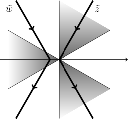
Figure 9. The integration contours for $\tilde{z}$ and $\tilde{w}$ in (3.12) leading to the Airy kernel approximation. Shaded are the regions where $\mathop{\mathrm{Re}}(\tilde{z}^{3})<0$.

Using (3.12) and Taylor expanding as $L\to+\infty$ we have

$$S_{L}(\mathfrak{z}_{L}+L^{-1/3}\mathfrak{c}_{L}^{-1}\tilde{z};t,N,\mathfrak{h}_{L}+\mathsf{h}L^{1/3}) =S_{L}(\mathfrak{z}_{L};t,N,\mathfrak{h}_{L})+\frac{\tilde{z}^{3}}{3}-\frac{\mathsf{h}\tilde{z}}{\mathfrak{z}_{L}\mathfrak{c}_{L}}$$

$$\hskip 70.0pt-L^{1/3}\mathsf{h}\log(-\mathfrak{z}_{L})+O(L^{-1/3}),$$

and similarly for the other term in the exponent in (3.11). Therefore, we have

$$K(t,N,x;t^{\prime},N^{\prime},x^{\prime})=\bigl{(}1+O(L^{-1/3})\bigr{)}(-\mathfrak{z}_{L})^{(\mathsf{h}^{\prime}-\mathsf{h})L^{1/3}}\frac{L^{-1/3}}{(-\mathfrak{z}_{L})\mathfrak{c}_{L}}\\ \times\frac{1}{(2\pi\mathbf{i})^{2}}\iint\frac{e^{\tilde{z}^{3}/3-\tilde{w}^{3}/3-(\mathfrak{z}_{L}\mathfrak{c}_{L})^{-1}\mathsf{h}\tilde{z}+(\mathfrak{z}_{L}\mathfrak{c}_{L})^{-1}\mathsf{h}^{\prime}\tilde{w}}d\tilde{z}\,d\tilde{w}}{\tilde{z}-\tilde{w}},$$

with $\tilde{z}$, $\tilde{w}$ contours as in Figure 9. This completes the proof. ∎

Lemma 3.10.

Under our assumptions on $(t(L),N(L))$, let $h=x+N$ and $h^{\prime}=x^{\prime}+N$ be such that $h^{\prime}-\mathfrak{h}_{L}(t,N)\leq-sL^{1/3}$ for some $s>0$. Then for some $C,c_{1},c_{2}>0$ and $L$ large enough we have

$$\bigl{|}K(t,N,x;t,N,x^{\prime})\bigr{|}\leq C(-\mathfrak{z}_{L}(t,N))^{h^{\prime}-h}\cdot\frac{e^{-c_{1}L^{1/3}}+e^{c_{2}(h^{\prime}-\mathfrak{h}_{L}(t,N))L^{-1/3}}}{\mathfrak{h}_{L}(t,N)-h^{\prime}+1}.$$

Proof.

First, observe that the assumptions imply that the double critical point $|\mathfrak{z}_{L}(t,N)|$ is uniformly bounded away from zero and infinity.

Write the kernel as (3.11) with integration contours described in Lemmas 3.6 and 3.7 and locally around $\mathfrak{z}_{L}$ in the proof of Lemma 3.9. In the exponent we have

$$\mathop{\mathrm{Re}}\bigl{[}S_{L}(z;t,N,h)-S_{L}(w;t,N,h^{\prime})\bigr{]}=(h^{\prime}-h)\log|\mathfrak{z}_{L}|+(h^{\prime}-\mathfrak{h}_{L})\log|w/\mathfrak{z}_{L}|\\ +\mathop{\mathrm{Re}}\bigl{[}S_{L}(z;t,N,\mathfrak{h}_{L})-S_{L}(w;t,N,\mathfrak{h}_{L})\bigr{]}.$$ (3.14)

If either $z$ or $w$ or both are outside of a $L^{-1/6}$-neighborhood of $\mathfrak{z}_{L}$, we estimate

$$\eqref{eq:K_outside_edge_proof1}\leq(h^{\prime}-h)\log|\mathfrak{z}_{L}|+(h^{\prime}-\mathfrak{h}_{L})\log|w/\mathfrak{z}_{L}|-cL^{1/3}$$ (3.15)

as in the proof of Lemma 3.9. The part in the exponent containing $w$ is integrable over the vertical $w$ contour, which leads to the first term in the estimate for $|K|$.

Now, if both $z,w$ are close to $\mathfrak{z}_{L}$, make the change of variables (3.12) and write

$$\eqref{eq:K_outside_edge_proof1}\leq(h^{\prime}-h)\log|\mathfrak{z}_{L}|+(h^{\prime}-\mathfrak{h}_{L})\Bigl{[}\frac{L^{-1/3}\mathop{\mathrm{Re}}\tilde{w}}{\mathfrak{z}_{L}\mathfrak{c}_{L}}+O(L^{-2/3})\Bigr{]}+\frac{1}{3}\mathop{\mathrm{Re}}\left[\tilde{z}^{3}-\tilde{w}^{3}\right].$$ (3.16)

The part containing $\tilde{z},\tilde{w}$ is integrable over the scaled contours in Figure 9. Since the coefficient by $\mathop{\mathrm{Re}}\tilde{w}$ is positive and $\mathop{\mathrm{Re}}\tilde{w}\leq-1$ on our contour, we estimate this integral using the exponential integral $\int_{1}^{\infty}e^{Au}du=e^{-A}/A$, where $u$ corresponds to $\mathop{\mathrm{Re}}\tilde{w}$, and $A$ is the coefficient by $\mathop{\mathrm{Re}}\tilde{w}$. This produces the second term in the estimate for $|K|$. This completes the proof. ∎

Proposition 3.11.

Under our assumptions on $(t(L),N(L))$, for fixed $\mathsf{y}\in\mathbb{R}$ and large enough $L$ we have

$$\mathbb{P}(h(t,N)>\mathfrak{h}_{L}(t,N)+\mathsf{y}L^{1/3})=\bigl{(}1+O(L^{-1/3})\bigr{)}F_{GUE}\bigl{(}-\mathsf{y}/\mathfrak{d}_{L}(t,N)\bigr{)},$$ (3.17)

where $\mathfrak{d}_{L}(t,N)$ is given by (3.9).

Proof.

Set $y:=\lfloor\mathfrak{h}_{L}(t,N)+\mathsf{y}L^{1/3}\rfloor-1$. Corollary 1.7 states that the probability in the left-hand side of (3.17) is given by a Fredholm determinant with expansion

$$1+\sum_{n=1}^{\infty}\frac{(-1)^{n}}{n!}\sum_{x_{1}=-\infty}^{y-N}\ldots\sum_{x_{n}=-\infty}^{y-N}\;\mathop{\mathrm{det}}_{i,j=1}^{n}\left[K(t,N,x_{i};t,N,x_{j})\right].$$ (3.18)

Fix $s>0$ (to be taken large later) and separate the terms in the above Fredholm expansion where all $x_{i}>y-N-sL^{1/3}$, plus the remainder. In the former terms we use Lemma 3.9, and the latter terms are smaller due to Lemma 3.10.

When all $x_{i}>y-N-sL^{1/3}\sim\mathfrak{h}_{L}-N+\mathsf{y}L^{1/3}-sL^{1/3}$, let us reparametrize the summation variables as $x_{i}=\mathfrak{h}_{L}-N+\mathsf{u}_{i}L^{1/3}$, with $\mathsf{u}_{i}\in\mathbb{R}$ going from $\mathsf{y}-s$ to $\mathsf{y}$ (in increments of $L^{-1/3}$). From Lemma 3.9 we have

$$\mathop{\mathrm{det}}_{i,j=1}^{n}\left[K(t,N,x_{i};t,N,x_{j})\right]=\bigl{(}1+O(L^{-1/3})\bigr{)}\left(\frac{L^{-1/3}}{\mathfrak{d}_{L}}\right)^{n}\mathop{\mathrm{det}}_{i,j=1}^{n}\Bigl{[}\mathsf{A}\Bigl{(}-\frac{\mathsf{u}_{i}}{\mathfrak{d}_{L}},-\frac{\mathsf{u}_{j}}{\mathfrak{d}_{L}}\Bigr{)}\Bigr{]},$$

and each $n$-fold sum over $x_{i}>\mathfrak{h}_{L}-N+(\mathsf{y}-s)L^{1/3}$ can be approximated (within $O(L^{-1/3})$ error) by the $n$-fold integral of the Airy kernel $\mathsf{A}$ from $-\mathsf{y}/\mathfrak{d}_{L}$ to $(s-\mathsf{y})/\mathfrak{d}_{L}$. Taking $s$ sufficiently large and using the decay of the Airy kernel (e.g., see [TW94]) leads to the GUE Tracy–Widom distribution function at $-\mathsf{y}/\mathfrak{d}_{L}$.

Consider now the remaining terms. Using Lemma 3.10 we have

$$(-\mathfrak{z}_{L})^{x+N-x^{\prime}-N^{\prime}}\sum_{x^{\prime}<\mathfrak{h}_{L}-N+(\mathsf{y}-s)L^{1/3}}|K(t,N,x;t^{\prime},N^{\prime},x^{\prime})|\\ \leq C_{1}e^{-c_{1}L^{1/3}}\log\bigl{(}L(s-\mathsf{y})\bigr{)}+(s-\mathsf{y})^{-1}C_{2}e^{-c_{2}(s-\mathsf{y})}\bigl{(}1+O(L^{-1/3})\bigr{)}$$

for some $C_{i},c_{i}>0$. The first term decays rapidly for large $L$, and the second term can be made small for fixed $\mathsf{y}$ by choosing a sufficiently large $s$.

Take the $n$-th term in (3.18) where some of the $x_{i}$’s are summed from $-\infty$ to $y-N-sL^{1/3}$, and expand the $n\times n$ determinant along a column $x_{j}$ corresponding to $x_{j}<\mathfrak{h}_{L}-N+(\mathsf{y}-s)L^{1/3}$. The resulting $n-1$ determinants are estimated via Hölder and Hadamard’s inequalities. Thus, the remaining terms in the Fredholm expansion are negligible and can be included in the error in the right-hand side of (3.17). This completes the proof. ∎

The final step of the proof of Theorem 1.14 (which would also imply Theorem 1.13) is to show that the approximation of the probability in Proposition 3.11 implies the convergence of the probabilities $\mathbb{P}(h(t,N)>L\mathfrak{h}(\tau,\eta)+\mathsf{y}L^{1/3})$ to the GUE Tracy–Widom distribution function. This convergence would clearly follow if

$$\mathfrak{h}_{L}(\tau L,\lfloor\eta L\rfloor)=L\mathfrak{h}(\tau,\eta)+o(L^{1/3}),\qquad\mathfrak{d}_{L}(\tau L,\lfloor\eta L\rfloor)=\mathfrak{d}(\tau,\eta)+o(1).$$ (3.19)

Observe that all sums in the definitions of $\mathfrak{z}_{L}$, $\mathfrak{h}_{L}$, $\mathfrak{d}_{L}$ in Section 3.2 are Riemann sums of the integrals from $0$ to $\eta$ from Section 1.5. The mesh of these integrals is of order $L^{-1}$, and due to the piecewise $C^{1}$ assumption on $\boldsymbol{\xi}(\cdot)$, integrals are approximated by Riemann sums within $O(L^{-1})$. This implies (3.19), which is the last step in the proof of Theorem 1.14.

Appendix A Checking the hydrodynamic equation

Here we check that the limiting density $\uprho(\tau,\eta)$ defined in Section 1.5 indeed satisfies the hydrodynamic equation (1.9). We assume that $\eta\geq\tau$ (since $\uprho\equiv 0$ clearly satisfies the equation), and use formulas (1.12) and (1.13). First, note that the initial condition $\uprho(0,\eta)=\mathbf{1}_{\eta\geq 0}$ corresponds to the solution $\mathfrak{z}(0,\eta)=-\infty$ of (1.12).

Observe that

$$\uprho(\tau,\eta)=\frac{\partial}{\partial\eta}\,\mathfrak{h}(\tau,\eta)=\frac{\mathfrak{z}^{2}(\tau,\eta)}{\left(\mathfrak{z}(\tau,\eta)-\boldsymbol{\xi}(\eta)\right)^{2}}-\mathfrak{z}_{\eta}(\tau,\eta)\int_{0}^{\eta}\frac{2\mathfrak{z}(\tau,\eta)\boldsymbol{\xi}(y)}{\left(\mathfrak{z}(\tau,\eta)-\boldsymbol{\xi}(y)\right)^{3}}\,dy.$$

The derivative $\mathfrak{z}_{\eta}$ can be found by differentiating (1.12) in $\eta$:

$$0=\frac{\boldsymbol{\xi}(\eta)}{\left(\mathfrak{z}(\tau,\eta)-\boldsymbol{\xi}(\eta)\right)^{2}}-\mathfrak{z}_{\eta}(\tau,\eta)\int_{0}^{\eta}\frac{2\boldsymbol{\xi}(y)}{\left(\mathfrak{z}(\tau,\eta)-\boldsymbol{\xi}(y)\right)^{3}}\,dy,$$

which immediately leads to $\uprho={\mathfrak{z}}/({\mathfrak{z}-\boldsymbol{\xi}(\eta)})$, which is formula (1.14) in the Introduction. This implies

$$\frac{\boldsymbol{\xi}(\eta)\uprho(\tau,\eta)}{1-\uprho(\tau,\eta)}=-\mathfrak{z}(\tau,\eta),\qquad\frac{\partial}{\partial\eta}\left(\frac{\boldsymbol{\xi}(\eta)\uprho(\tau,\eta)}{1-\uprho(\tau,\eta)}\right)=-\mathfrak{z}_{\eta}(\tau,\eta).$$

The remaining term $\uprho_{\tau}$ in (1.9) can be expressed through $\mathfrak{z}_{\tau}$ by differentiating (1.12) in $\tau$. We have

$$1=-\mathfrak{z}_{\tau}(\tau,\eta)\int_{0}^{\eta}\frac{2\boldsymbol{\xi}(y)}{\left(\mathfrak{z}(\tau,\eta)-\boldsymbol{\xi}(y)\right)^{3}}\,dy,$$

and

$$\uprho_{\tau}(\tau,\eta)=\frac{\partial}{\partial\tau}\left(\frac{\mathfrak{z}(\tau,\eta)}{\mathfrak{z}(\tau,\eta)-\boldsymbol{\xi}(\eta)}\right)=-\mathfrak{z}_{\tau}(\tau,\eta)\,\frac{\boldsymbol{\xi}(\eta)}{\left(\mathfrak{z}(\tau,\eta)-\boldsymbol{\xi}(\eta)\right)^{2}}.$$

Combining the above formulas yields the hydrodynamic equation (1.9) for the limiting density.

Remark A.1 (Homogeneous case).

For $\boldsymbol{\xi}(\eta)\equiv 1$ equation (1.9) looks as $\tau=\eta/(z-1)^{2}$, and its unique negative root is $\mathfrak{z}(\tau,\eta)=1-\sqrt{\eta/\tau}$, $\eta\geq\tau$ (note that in the homogeneous case $\tau_{e}(\eta)=\eta$). This leads to $\uprho(\tau,\eta)={\mathfrak{z}(\tau,\eta)}/({\mathfrak{z}(\tau,\eta)-1)}=1-\sqrt{\tau/\eta}$, and so the height function is $\mathfrak{h}(\tau,\eta)=\left(\sqrt{\eta}-\sqrt{\tau}\right)^{2}$, as mentioned in Remark 1.9 in the Introduction.

Department of Mathematics, University of Virginia, Charlottesville, VA 22904, and Institute for Information Transmission Problems, Moscow, Russia 127051

E-mail address: lenia.petrov@gmail.com

References

- [AG05] E. Andjel and H. Guiol, Long-range exclusion processes, generator and invariant measures, Ann. Probab. 33 (2005), no. 6, 2314–2354, arXiv:math/0411655 [math.PR].
- [AK84] E. Andjel and C. Kipnis, Derivation of the hydrodynamical equation for the zero-range interaction process, Ann. Probab. 12 (1984), no. 2, 325–334.
- [Ass20] T. Assiotis, Determinantal structures in space inhomogeneous dynamics on interlacing arrays, Ann. Inst. H. Poincaré 21 (2020), 909–940, arXiv:1910.09500 [math.PR].
- [Bai06] J. Baik, Painlevé formulas of the limiting distributions for nonnull complex sample covariance matrices, Duke Math J. 133 (2006), no. 2, 205–235, arXiv:math/0504606 [math.PR].
- [Bar01] Yu. Baryshnikov, GUEs and queues, Probab. Theory Relat. Fields 119 (2001), 256–274.
- [BBW18] A. Borodin, A. Bufetov, and M. Wheeler, Between the stochastic six vertex model and hall-littlewood processes, Duke Math. J. 167 (2018), no. 13, 2457–2529, arXiv:1611.09486 [math.PR].
- [BC14] A. Borodin and I. Corwin, Macdonald processes, Probab. Theory Relat. Fields 158 (2014), 225–400, arXiv:1111.4408 [math.PR].
- [BCG16] A. Borodin, I. Corwin, and V. Gorin, Stochastic six-vertex model, Duke J. Math. 165 (2016), no. 3, 563–624, arXiv:1407.6729 [math.PR].
- [BDJ99] J. Baik, P. Deift, and K. Johansson, On the distribution of the length of the longest increasing subsequence of random permutations, Jour. AMS 12 (1999), no. 4, 1119–1178, arXiv:math/9810105 [math.CO].
- [BF08] A. Borodin and P. Ferrari, Large time asymptotics of growth models on space-like paths I: PushASEP, Electron. J. Probab. 13 (2008), 1380–1418, arXiv:0707.2813 [math-ph].
- [BF14] by same author, Anisotropic growth of random surfaces in 2+1 dimensions, Commun. Math. Phys. 325 (2014), 603–684, arXiv:0804.3035 [math-ph].
- [BFS08] A. Borodin, P. Ferrari, and T. Sasamoto, Large Time Asymptotics of Growth Models on Space-like Paths II: PNG and Parallel TASEP, Commun. Math. Phys. 283 (2008), no. 2, 417–449, arXiv:0707.4207 [math-ph].
- [BFS09] by same author, Two speed tasep, J. Stat. Phys 137 (2009), no. 5, 936–977, arXiv:0904.4655 [math-ph].
- [BG13] A. Borodin and V. Gorin, Markov processes of infinitely many nonintersecting random walks, Probab. Theory Relat. Fields 155 (2013), no. 3-4, 935–997, arXiv:1106.1299 [math.PR].
- [BM18] A. Bufetov and K. Matveev, Hall-littlewood rsk field, Selecta Math. 24 (2018), no. 5, 4839–4884, arXiv:1705.07169 [math.PR].
- [BMP19] A. Bufetov, M. Mucciconi, and L. Petrov, Yang-baxter random fields and stochastic vertex models, arXiv preprint (2019), arXiv:1905.06815 [math.PR]. To appear in Adv. Math.
- [BOO00] A. Borodin, A. Okounkov, and G. Olshanski, Asymptotics of Plancherel measures for symmetric groups, Jour. AMS 13 (2000), no. 3, 481–515, arXiv:math/9905032 [math.CO].
- [Bor10] Folkmar Bornemann, On the numerical evaluation of Fredholm determinants, Math. Comp. 79 (2010), no. 270, 871–915, arXiv:0804.2543 [math.NA].
- [Bor11] A. Borodin, Determinantal point processes, Oxford Handbook of Random Matrix Theory (G. Akemann, J. Baik, and P. Di Francesco, eds.), Oxford University Press, 2011, arXiv:0911.1153 [math.PR].
- [Bor18] by same author, Stochastic higher spin six vertex model and macdonald measures, Jour. Math. Phys. 59 (2018), no. 2, 023301, arXiv:1608.01553 [math-ph].
- [BP16] A. Borodin and L. Petrov, Nearest neighbor Markov dynamics on Macdonald processes, Adv. Math. 300 (2016), 71–155, arXiv:1305.5501 [math.PR].
- [BP18] by same author, Inhomogeneous exponential jump model, Probab. Theory Relat. Fields 172 (2018), 323–385, arXiv:1703.03857 [math.PR].
- [BP19] A. Bufetov and L. Petrov, Yang-Baxter field for spin Hall-Littlewood symmetric functions, Forum Math. Sigma 7 (2019), e39, arXiv:1712.04584 [math.PR].
- [BSS14] R. Basu, V. Sidoravicius, and A. Sly, Last passage percolation with a defect line and the solution of the slow bond problem, arXiv preprint (2014), arXiv:1408.3464 [math.PR].
- [BSS17] R. Basu, S. Sarkar, and A. Sly, Invariant measures for tasep with a slow bond, arXiv preprint (2017), arXiv:1704.07799.
- [Cal15] J. Calder, Directed last passage percolation with discontinuous weights, Jour. Stat. Phys. 158 (2015), no. 4, 903–949.
- [Cor12] I. Corwin, The Kardar-Parisi-Zhang equation and universality class, Random Matrices Theory Appl. 1 (2012), 1130001, arXiv:1106.1596 [math.PR].
- [DF90] P. Diaconis and J.A. Fill, Strong stationary times via a new form of duality, Ann. Probab. 18 (1990), 1483–1522.
- [DLSS91] B. Derrida, J. Lebowitz, E. Speer, and H. Spohn, Dynamics of an anchored Toom interface, J. Phys. A 24 (1991), no. 20, 4805.
- [Dui13] M. Duits, The Gaussian free field in an interlacing particle system with two jump rates, Comm. Pure Appl. Math. 66 (2013), no. 4, 600–643, arXiv:1105.4656 [math-ph].
- [DW08] A.B. Dieker and J. Warren, Determinantal transition kernels for some interacting particles on the line, Annales de l’Institut Henri Poincaré 44 (2008), no. 6, 1162–1172, arXiv:0707.1843 [math.PR].
- [Fer08] P. Ferrari, The universal Airy1 and Airy2 processes in the Totally Asymmetric Simple Exclusion Process, Integrable Systems and Random Matrices: In Honor of Percy Deift (J. Baik, T. Kriecherbauer, L.-C. Li, K. T.-R. McLaughlin, and C. Tomei, eds.), Contemporary Math., AMS, 2008, arXiv:math-ph/0701021, pp. 321–332.
- [FS03] P. Ferrari and H. Spohn, Step fluctuations for a faceted crystal, J. Stat. Phys 113 (2003), no. 1, 1–46, arXiv:cond-mat/0212456 [cond-mat.stat-mech].
- [Gho17] P. Ghosal, Hall-Littlewood-PushTASEP and its KPZ limit, arXiv preprint (2017), arXiv:1701.07308 [math.PR].
- [GKS10] N. Georgiou, R. Kumar, and T. Seppäläinen, TASEP with discontinuous jump rates, ALEA Lat. Am. J. Probab. Math. Stat. 7 (2010), 293–318, arXiv:1003.3218 [math.PR].
- [GS92] L.-H. Gwa and H. Spohn, Six-vertex model, roughened surfaces, and an asymmetric spin Hamiltonian, Phys. Rev. Lett. 68 (1992), no. 6, 725–728.
- [Gui97] H. Guiol, Un résultat pour le processus d’exclusion à longue portée [a result for the long-range exclusion process], Annales de l’Institut Henri Poincare (B) Probability and Statistics, vol. 33, 1997, pp. 387–405.
- [HKPV06] J.B. Hough, M. Krishnapur, Y. Peres, and B. Virág, Determinantal processes and independence, Probability Surveys 3 (2006), 206–229, arXiv:math/0503110 [math.PR].
- [Joh00] K. Johansson, Shape fluctuations and random matrices, Commun. Math. Phys. 209 (2000), no. 2, 437–476, arXiv:math/9903134 [math.CO].
- [KPS19] A. Knizel, L. Petrov, and A. Saenz, Generalizations of tasep in discrete and continuous inhomogeneous space, Commun. Math. Phys. 372 (2019), 797–864, arXiv:1808.09855 [math.PR].
- [Lan96] C. Landim, Hydrodynamical limit for space inhomogeneous one-dimensional totally asymmetric zero-range processes, Ann. Probab. 24 (1996), no. 2, 599–638.
- [Lig05] T. Liggett, Interacting Particle Systems, Springer-Verlag, Berlin, 2005.
- [Mac95] I.G. Macdonald, Symmetric functions and Hall polynomials, 2nd ed., Oxford University Press, 1995.
- [MG69] C. MacDonald and J. Gibbs, Concerning the kinetics of polypeptide synthesis on polyribosomes, Biopolymers 7 (1969), no. 5, 707–725.
- [MGP68] C. MacDonald, J. Gibbs, and A. Pipkin, Kinetics of biopolymerization on nucleic acid templates, Biopolymers 6 (1968), no. 1, 1–25.
- [O’C03a] N. O’Connell, A path-transformation for random walks and the Robinson-Schensted correspondence, Trans. AMS 355 (2003), no. 9, 3669–3697.
- [O’C03b] by same author, Conditioned random walks and the RSK correspondence, J. Phys. A 36 (2003), no. 12, 3049–3066.
- [Oko01] A. Okounkov, Infinite wedge and random partitions, Selecta Math. 7 (2001), no. 1, 57–81, arXiv:math/9907127 [math.RT].
- [Oko02] by same author, Symmetric functions and random partitions, Symmetric functions 2001: Surveys of Developments and Perspectives (S. Fomin, ed.), Kluwer Academic Publishers, 2002, arXiv:math/0309074 [math.CO].
- [OP13] N. O’Connell and Y. Pei, A q-weighted version of the Robinson-Schensted algorithm, Electron. J. Probab. 18 (2013), no. 95, 1–25, arXiv:1212.6716 [math.CO].
- [OR03] A. Okounkov and N. Reshetikhin, Correlation function of Schur process with application to local geometry of a random 3-dimensional Young diagram, Jour. AMS 16 (2003), no. 3, 581–603, arXiv:math/0107056 [math.CO].
- [PS02] M. Prähofer and H. Spohn, Scale invariance of the PNG droplet and the Airy process, J. Stat. Phys. 108 (2002), 1071–1106, arXiv:math.PR/0105240.
- [QS15] J. Quastel and H. Spohn, The one-dimensional KPZ equation and its universality class, J. Stat. Phys 160 (2015), no. 4, 965–984, arXiv:1503.06185 [math-ph].
- [Rez91] F. Rezakhanlou, Hydrodynamic limit for attractive particle systems on , Commun. Math. Phys. 140 (1991), no. 3, 417–448.
- [Ros81] H. Rost, Nonequilibrium behaviour of a many particle process: density profile and local equilibria, Z. Wahrsch. Verw. Gebiete 58 (1981), no. 1, 41–53.
- [RS05] A. Rákos and G. Schütz, Current distribution and random matrix ensembles for an integrable asymmetric fragmentation process, J. Stat. Phys 118 (2005), no. 3-4, 511–530, arXiv:cond-mat/0405464 [cond-mat.stat-mech].
- [RT08] L. Rolla and A. Teixeira, Last passage percolation in macroscopically inhomogeneous media, Electron. Commun. Probab. 13 (2008), 131–139.
- [Sep99] T. Seppäläinen, Existence of hydrodynamics for the totally asymmetric simple k-exclusion process, Ann. Probab. 27 (1999), no. 1, 361–415.
- [Sim05] B. Simon, Trace ideals and their applications, second edition, Mathematical Surveys and Monographs, vol. 120, AMS, 2005.
- [Sos00] A. Soshnikov, Determinantal random point fields, Russian Mathematical Surveys 55 (2000), no. 5, 923–975, arXiv:math/0002099 [math.PR].
- [Spi70] F. Spitzer, Interaction of Markov processes, Adv. Math. 5 (1970), no. 2, 246–290.
- [TW93] C. Tracy and H. Widom, Level-spacing distributions and the Airy kernel, Physics Letters B 305 (1993), no. 1, 115–118, arXiv:hep-th/9210074.
- [TW94] by same author, Level-spacing distributions and the Airy kernel, Commun. Math. Phys. 159 (1994), no. 1, 151–174, arXiv:hep-th/9211141.
- [VK86] A. Vershik and S. Kerov, The characters of the infinite symmetric group and probability properties of the Robinson-Shensted-Knuth algorithm, SIAM J. Alg. Disc. Math. 7 (1986), no. 1, 116–124.