Modeling of depth-induced wave breaking in a fully nonlinear free-surface potential flow model

Abstract

Two methods to treat wave breaking in the framework of the Hamiltonian formulation of free-surface potential flow are presented, tested, and validated. The first is an extension of Kennedy et al. (2000)’s eddy-viscosity approach originally developed for Boussinesq-type wave models. In this approach, an extra term, constructed to conserve the horizontal momentum for waves propagating over a flat bottom, is added in the dynamic free-surface condition. In the second method, a pressure distribution is introduced at the free surface that dissipates wave energy by analogy to a hydraulic jump (Guignard and Grilli, 2001). The modified Hamiltonian systems are implemented using the Hamiltonian Coupled-Mode Theory, in which the velocity potential is represented by a rapidly convergent vertical series expansion. Wave energy dissipation and conservation of horizontal momentum are verified numerically. Comparisons with experimental measurements are presented for the propagation of a breaking dispersive shock wave following a dam break, and then incident regular waves breaking on a mildly sloping beach and over a submerged bar.

Keywords: wave breaking, Hamiltonian formulation of water waves, eddy-viscosity, fully nonlinear water waves

Highlights

• Two wave breaking techniques are tested in a fully nonlinear model.

• Breaking is implemented by extending the Hamiltonian Coupled-Mode Theory.

• Energy dissipation and horizontal momentum conservation are verified numerically.

• Good performance is shown in the presence of nonlinearity, dispersion and breaking.

• Both methods can be implemented in other free-surface potential flow models.

1 Introduction

The continuous rise of human activity in coastal areas significantly motivates the development of numerical models able to predict complex nearshore wave dynamics. Accurate knowledge of evolving wave fields is particularly useful in the study of sediment transport and beach erosion, and in the design of marine renewable energy systems. Challenging issues that must be considered include strongly nonlinear wave propagation, dispersive effects, and complex wave-seabed interactions. In addition, a reliable model should provide accurate predictions of breaking waves and their post-breaking evolution.

Physically precise simulations of unsteady wave propagation, including breaking, can be achieved by solving the primitive Navier-Stokes equations. Although possible, this approach has a high computational cost and its application for large spatial domains (e.g. scales of kilometeres) is cumbersome. Therefore, a widely used approach for simulating coastal waves is the adoption of the physical framework of free-surface potential flow (FSPF) and the derivation of model equations via asymptotic arguments or depth integration. This line of work is mainly represented by Boussinesq-type (BT) models (see e.g. Nwogu (1993); Karambas and Memos (2009); Madsen et al. (2006)) and the reviews of Brocchini (2013); Kirby (2016)), and Green-Nagdhi (GN) equations (see e.g. Lannes and Bonneton (2009); Chazel et al. (2011); Zhao et al. (2014); Mitsotakis et al. (2015)). Another class of models that use pertubative calculations is based on the High-Order Spectral (HOS) method (Dommermuth and Yue, 1987; Craig and Sulem, 1993; Guyenne and Nicholls, 2007; Gouin et al., 2016). Direct methods of solution of fully nonlinear FSPF equations have also been proposed (Bingham and Zhang, 2007; Gagarina et al., 2014; Grilli et al., 2001). An alternative approach that treats the fully nonlinear problem is the Hamiltonian Coupled-Mode Theory or HCMT. Like other direct methods of solution, HCMT is a reformulation of FSPF without any simplification concerning nonlinearity, dispersion or seabed deformation. This is achieved through a rapidly convergent vertical series expansion of the velocity potential that is valid in the entire non-uniform fluid domain up to the boundaries (Belibassakis and Athanassoulis, 2011; Athanassoulis and Papoutsellis, 2017). The resulting equations retain the dimensionally-reduced Hamiltonian structure of the water wave system (Zakharov, 1968; Craig and Sulem, 1993) and give accurate predictions of fully nonlinear and strongly dispersive waves over variable bathymetry up to breaking (Athanassoulis and Papoutsellis, 2015; Papoutsellis and Athanassoulis, 2017; Athanassoulis et al., 2017; Papoutsellis et al., 2018). Wave models with similar mathematical structure and capabilities have also been developed using Chebyshev series representations of the potential in the vertical direction (Tian and Sato, 2008; Yates and Benoit, 2015; Raoult et al., 2016, 2019). The purpose of this paper is to extend the domain of application of fully nonlinear potential flow models by incorporating wave-breaking effects. Here, the modeling strategies are implemented and tested using HCMT.

Most previous work attempts to incorporate wave breaking into BT or GN models by introducing dissipation mechanisms that are applied throughout breaking events. This is consistent with the fact that wave breaking results in wave energy dissipation. This approach thus avoids the direct fine-scale computations of the turbulent wave motion encountered during breaking and parametrizes the effects of wave breaking on the wave kinematics. The simulated decrease in wave energy suppresses overturning of the free surface allowing the wave form (and simulation) to remain stable. Implementation of such an approach requires (i) the addition of an extra dissipative term to the otherwise inviscid evolution equations and (ii) the adoption of a breaking criterion to determine when the dissipative term will be activated (beginning of breaking) and de-activated (end of breaking). Concerning the extra terms, two dominant strategies can be identified: the Eddy Viscosity Model (Heitner and Housner, 1970; Zelt, 1991; Karambas and Koutitas, 1992; Kennedy et al., 2000) and the Surface Roller Model (Svendsen, 1984; Schäffer et al., 1993; Madsen et al., 1997).

In the eddy viscosity approach, a diffusion term is added to the momentum equation. It is controlled by an eddy viscosity coefficient that depends on a mixing length parameter that is used to calibrate the approach in comparison to experimental measurements. Cienfuegos et al. (2010) proposed an improvement by adding an extra ad hoc diffusive term to the mass equation to improve the simulated horizontal asymmetry in the inner surf zone. Kurnia and van Groesen (2014) also proposed a variant of Kennedy et al. (2000)’s approach applicable to fully dispersive waves described by a high-order Hamiltonian model. Recently, Kazolea and Ricchiuto (2018) proposed an alternative approach in which the eddy viscosity is calculated in terms of an additional partial differential equation for the turbulent kinetic energy. Finally, an eddy viscosity approach for deep water breaking using the HOS method was presented in Tian et al. (2010) and Seiffert and Ducrozet (2017).

In the second approach, the surface roller concept asserts that a breaking wave is divided into a potential core and a turbulent region close to the wave front. By prescribing horizontal velocity profiles in these regions, an extra term is derived in the momentum equation. Dissipation depends on several geometric parameters, such as the roller thickness and the mean front slope of the breaking wave. Advanced versions of this approach that take into account rotational effects have also been proposed (Veeramony and Svendsen, 2000; Briganti et al., 2004).

A new Hybrid approach has also gained popularity due to its relative simplicity. In this technique, instead of adding an extra term that dissipates wave energy, BT or GN models are locally transformed into the nonlinear shallow water (NSW) equations by suppression of the dispersive terms. This allows breaking waves (detected by an appropriate criterion) to be propagated as shocks (Tonelli and Petti, 2009; Roeber et al., 2010; Bonneton et al., 2011; Tissier et al., 2012; Kazolea et al., 2014; Kazolea and Ricchiuto, 2018). The advantage of this approach is that no additional ad-hoc dissipative terms are required, thus the breaking dissipation introduced in the model has no free parameters requiring calibration.

In the framework of fully nonlinear FSPF, the development of dissipation mechanisms that model wave breaking has not yet been studied thoroughly. A notable exception is the boundary element implementation of Guignard and Grilli (2001) and Grilli et al. (2019) in which a dissipative pressure distribution is introduced in the dynamic free-surface boundary condition (FSBC). It is constructed so that the energy dissipated is proportional to the energy dissipated by a hydraulic jump with characteristics similar to those of the breaking wave.

The goal of this study is to address this lack of progress by implementing two wave breaking techniques in the framework of the Hamiltonian formulation of FSPF. The first is an eddy viscosity approach following Kennedy et al. (2000). The main difficulty here and the primary difference of the current approach relative to previous work is that the dynamic FSBC is an evolution equation of the free-surface velocity potential rather than the (depth-integrated) horizontal velocity used in BT or GN models. The second method uses the dissipative pressure distribution proposed in Guignard and Grilli (2001). The two methods are incorporated in a numerical scheme for HCMT (Papoutsellis et al., 2018). In principle, the presented techniques can be applied to other numerical models provided that the dynamic FSBC is cast in terms of the free-surface potential (e.g. Bingham and Zhang (2007); Gagarina et al. (2014); Grilli et al. (2001); Raoult et al. (2016); Gouin et al. (2016)).

The organisation of the paper is as follows: in Section 2, the governing equations of free surface potential flow and its Hamiltonian structure are outlined. In Section 3, the breaking initiation criterion and the two wave breaking dissipation techniques are introduced. Section 4 presents briefly the HCMT and extends the numerical scheme of Papoutsellis et al. (2018) to the breaking case studied herein. Numerical verifications and validations are presented in Section 5, before a discussion of the results and conclusions are detailed in Section 6.

2 Free-surface potential flow modeling

2.1 Governing equations

The FSPF equations describe the irrotational motion of an inviscid, incompressible fluid with a free surface under the influence of gravity. In a two-dimensional Cartesian coordinate system $(x,z)$, with the vertical coordinate $z$ pointing upwards, the fluid occupies a region delimited by the time-dependent free surface at $z=\eta(x,t)$ and the fixed bottom at $z=-h(x)$, $h(x)>0$. The free-surface elevation $\eta$ and bottom bathymetry $h$ are assumed to be smooth, single-valued functions such that $\eta(x,t)+h(x)>0$, thus excluding overturning waves and the representation of the shoreline. Fluid flow is described in terms of the velocity potential $\Phi(x,z,t)$ and free-surface elevation $\eta(x,t)$ by the equations, e.g. (Stoker, 1957)

$$\partial_{t}\eta+\partial_{x}\eta\partial_{x}\Phi-\partial_{z}\Phi =0,\,\,\,\,\text{on}\,\,z=\eta(x,t),$$ (2.1a)

$$\partial_{t}\Phi+\frac{1}{2}(\partial_{x}\Phi)^{2}+\frac{1}{2}(\partial_{z}\Phi)^{2}+g\eta =-P_{\text{surf}},\,\,\,\text{on}\,\,z=\eta(x,t),$$ (2.1b)

$$\partial_{x}^{2}\Phi+\partial_{z}^{2}\Phi =0,\,\,\,\,\text{in}\,\,-h(x)\leq z\leq\eta(x,t),$$ (2.1c)

$$\partial_{x}h\partial_{x}\Phi+\partial_{z}\Phi =0,\,\,\,\,\text{on}\,\,z=-h(x),$$ (2.1d)

where $g$ is the acceleration of gravity, and $P_{\text{surf}}$ denotes the pressure acting on the free surface. It is also assumed that $\eta$, $\Phi$, and their derivatives vanish at infinity. Zakharov (1968) observed that the kinematic and dynamic FSBCs, Eqs. (2.1a) and (2.1b), can be written equivalently as a system of evolution equations of the free-surface elevation $\eta(x,{\kern 1.0pt}t)$ and the trace of wave potential on $z=\eta(x,{\kern 1.0pt}t)$,

$$\psi(x,{\kern 1.0pt}t):=\Phi(x,{\kern 1.0pt}z=\eta(x,{\kern 1.0pt}t),{\kern 1.0pt}t).$$ (2.2)

This system takes the form

$$\partial_{t}\eta =\mathcal{G}[\eta,h]\psi,$$ (2.3a)

$$\partial_{t}\psi =-g\eta-\frac{1}{2}(\partial_{x}\psi)^{2}+\frac{\big{(}\mathcal{G}[\eta,h]\psi+\partial_{x}\psi\partial_{x}\eta\big{)}^{2}}{2\left(1+|\partial_{x}\eta|^{2}\right)}-P_{\text{surf}},$$ (2.3b)

where ${\rm{\mathcal{G}}}{\kern 1.0pt}[\eta,h]\psi$ is the Dirichlet-to-Neumann (DtN) operator introduced by Craig and Sulem (1993). It is defined by

$${\rm{\mathcal{G}}}[\eta,h]{\kern 1.0pt}\psi=-\partial_{x}\eta{\kern 1.0pt}\left[{\kern 1.0pt}\partial_{x}\Phi\right]_{{\kern 1.0pt}z{\kern 1.0pt}={\kern 1.0pt}\eta}+\left[{\kern 1.0pt}\partial_{z}\Phi\right]_{{\kern 1.0pt}z{\kern 1.0pt}={\kern 1.0pt}\eta},$$ (2.4)

where $\Phi$ is determined by the boundary value problem consisting of the Laplace equation (2.1c) together with the impermeability condition on the seabed, Eq. (2.1d), and the Dirichlet condition, Eq. (2.2). In Section 3, specific forms of $P_{\text{surf}}$ that model wave-breaking dissipation will be presented. Prior to that, it is instructive to briefly present the conservation of three important quantities when $P_{\text{surf}}\equiv 0$, namely the total energy, mass and horizontal momentum.

2.2 Hamiltonian structure and conserved quantities

In the absence of surface pressure, the water wave system (2.3) is equivalent with the Hamiltonian formulation (Zakharov, 1968; Broer, 1974; Miles, 1977)

$$\partial_{t}\eta =\delta_{\psi}\mathcal{H}=\mathcal{G}[\eta,h]\psi,$$ (2.5a)

$$\partial_{t}\psi =-\delta_{\eta}\mathcal{H}=-g\eta-\frac{1}{2}(\partial_{x}\psi)^{2}+\frac{\big{(}\mathcal{G}[\eta,h]\psi+\partial_{x}\psi\partial_{x}\eta\big{)}^{2}}{2\left(1+|\partial_{x}\eta|^{2}\right)},$$ (2.5b)

where $\delta_{\eta}:=\delta/\delta\eta$ and $\delta_{\psi}:=\delta/\delta\psi$ denote variational derivatives, and the Hamiltonian $\mathcal{H}=\mathcal{H}[\eta,\psi](t)$ is the functional of the total (kinetic and potential) wave energy

$$\begin{aligned} \mathcal{H}[\eta,\psi](t)=\int E(\eta,\psi)\,dx,\quad E(\eta,\psi)=\frac{1}{2}\left(\psi\mathcal{G}[\eta,h]\psi+g\eta^{2}\right).\end{aligned}$$ (2.6)

The systematic derivation of conserved quantities associated with solutions $(\eta,\psi)$ of the above system is presented in Benjamin and Olver (1982). Conservation of energy, mass and momentum are verified explicitly below because these calculations will be used in the next section.

Conservation of energy is a well-known property of the Hamiltonian structure (2.5),(2.6): the time derivative of $\mathcal{H}(\eta,\psi)$ is

$$\frac{d\mathcal{H}}{dt}=\int\big{(}\delta_{\psi}\mathcal{H}\partial_{t}\psi+\delta_{\eta}\mathcal{H}\partial_{t}\eta\big{)}dx=\int\big{(}-\delta_{\psi}\mathcal{H}\delta_{\eta}\mathcal{H}+\delta_{\eta}\mathcal{H}\delta_{\psi}\mathcal{H}\big{)}dx=0,$$ (2.7)

after using the first equalities of Eqs. (2.5). For the mass,

$$\mathcal{M}=\int\eta dx,$$ (2.8)

the time derivative is

$$\frac{d\mathcal{M}}{dt}=\int\partial_{t}\eta dx=\int G[\eta,h]\psi dx=0,$$

where the last equality is obtained after invoking the self-adjointness of the operator i.e. $\mathcal{G}[\eta,h]$, $\int G[\eta,h]u\,vdx=\int G[\eta,h]v\,udx$ for all $u$, $v$ (Milder, 1990; Lannes, 2013), in conjunction with the fact that $\mathcal{G}[\eta,h]1=0$. Finally, the horizontal momentum in the case of a flat bottom, $\partial_{x}h=0$, is (Benjamin and Olver, 1982)

$$\mathcal{I}(\eta,\psi)=-\int\partial_{x}\eta\,\psi\,dx.$$ (2.9)

The time derivative of functional $\mathcal{I}$ is thus

$$\begin{aligned} \frac{d\mathcal{I}}{dt}=-\int\Big{(}\partial_{xt}^{2}\eta\psi+\partial_{x}\eta\partial_{t}\psi\Big{)}dx=-\int\Big{(}-\partial_{t}\eta\partial_{x}\psi+\partial_{x}\eta\partial_{t}\psi\Big{)}dx,\end{aligned}$$ (2.10)

where integration by parts has been used for the first term in conjunction with the assumption that the temporal derivative of the free-surface elevation vanishes at infinity. Substituting the Hamiltonian equations (2.5) in Eq. (2.10), $d\mathcal{I}/dt$ is written

$$\frac{d\mathcal{I}}{dt}=\int\Big{(}\delta_{\psi}\mathcal{H}\partial_{x}\psi+\delta_{\eta}\mathcal{H}\partial_{x}\eta\Big{)}dx,$$ (2.11)

and the identity

$$\int\partial_{x}Edx=\int\Big{(}\delta_{\psi}\mathcal{H}\partial_{x}\psi+\delta_{\eta}\mathcal{H}\partial_{x}\eta\Big{)}dx,$$ (2.12)

proven in A, yields

$$d\mathcal{I}/dt=0,$$ (2.13)

since $E$, given by Eq. (2.6), vanishes at infinity. Here it is thus proven that the total mass, energy and horizontal momentum (in the case of uniform water depth) are all constant in time.

3 Wave-breaking models

To take into account the effects of wave breaking, the modified water-wave system is:

$$\partial_{t}\eta =\delta_{\psi}\mathcal{H},$$ (3.1a)

$$\partial_{t}\psi =-\delta_{\eta}\mathcal{H}-P_{\text{surf}},$$ (3.1b)

where $P_{\text{surf}}=P_{\text{surf}}(x,t)$ is activated from the initial time of breaking, $t_{i}$, until the cessation time of breaking, $t_{f}$, over a spatial breaking region $\Theta$, which also varies in time. The domains $\Theta$ and $[t_{i},t_{f}]$ are determined during the wave evolution on the basis of empirical criteria described in Sections 3.1 and 3.2. It should be noted that the expressions of the total energy, mass, and horizontal momentum do not change and are still defined by Eqs. (2.6), (2.8) and (2.9), respectively.

The effect of $P_{\text{surf}}$ on the rate of change of total energy becomes apparent by calculating the time derivative of the Hamiltonian functional (2.6) by taking into account Eqs. (3.1) such that

$$\frac{d\mathcal{H}}{dt}=\int\big{(}\delta_{\eta}\mathcal{H}\partial_{t}\eta+\delta_{\psi}\mathcal{H}\partial_{t}\psi\big{)}d\textbf{x}=\int\big{(}\left(-\partial_{t}\psi-P_{\text{surf}}\right)\partial_{t}\eta+\partial_{t}\eta\partial_{t}\psi\big{)}d\textbf{x},$$

and thus,

$$\frac{d\mathcal{H}}{dt}=-\int_{\Theta}P_{\text{surf}}\,\partial_{t}\eta\,dx=-\int_{\Theta}P_{\text{surf}}\,G[\eta,h]\psi\,dx.$$ (3.2)

The expression for the rate of change of mass remains unchanged and still equals zero. For the rate of change of horizontal momentum of the modified system (3.1), Eqs. (2.10) and (3.1) are used to calculate

$$\frac{d\mathcal{I}}{dt}=\int\Big{(}\partial_{t}\,\eta\partial_{x}\psi-\partial_{x}\eta\,\partial_{t}\psi\Big{)}dx=\int\big{(}\delta_{\psi}\mathcal{H}\partial_{x}\psi+\delta_{\eta}\mathcal{H}\partial_{x}\eta+P_{\text{surf}}\,\partial_{x}\eta\big{)}dx.$$ (3.3)

Using Eq. (2.12), the first two terms in the right hand side of Eq. (3.3) vanish leading to

$$\begin{aligned} \frac{d\mathcal{I}}{dt}=\int_{\Theta}P_{\text{surf}}\,\partial_{x}\eta\,dx.\end{aligned}$$ (3.4)

Eqs. (3.2) and (3.4) are the starting point for the construction of $P_{\text{surf}}$.

3.1 Eddy Viscosity Model (EVM)

In the eddy viscosity approach, $P_{\text{surf}}$ is constructed with the requirement that the momentum $\mathcal{I}=\mathcal{I}(\eta,\psi)$, Eq. (2.9), remains invariant over a flat bottom. As noted by Kennedy et al. (2000), this feature of horizontal momentum conservation is consistent with the analogy between breaking bores and breaking waves. Using Eq. (3.4), it is not straightforward to determine $P_{\text{surf}}$ to enforce the condition $d\mathcal{I}/dt=0$. Nonetheless, by assuming that $P_{\text{surf}}$ vanishes at the boundary of the breaking region $\Theta$ and that the bottom is flat ($\partial_{x}h=0$), an integration by parts gives

$$\begin{aligned} \frac{d\mathcal{I}}{dt}=-\int_{\Theta}\partial_{x}P_{\text{surf}}\,H\,dx,\end{aligned}$$ (3.5)

where $H=\eta+h$ is the total water depth. Following Kurnia and van Groesen (2014), $P_{\text{surf}}$ is chosen here such that

$$\partial_{x}P_{\text{surf}}=\frac{1}{H}\partial_{x}F,\quad\text{with}\quad F=0\quad\text{outside}\,\,\Theta,$$ (3.6)

which yields $d\mathcal{I}/dt=\int_{\Theta}\partial_{x}F=0$. Function $F$ is given by

$$F=\nu\,G[\eta,h]\psi,$$ (3.7)

where $\nu=\nu(x,t)$ is the eddy viscosity coefficient assumed to be of the form:

$$\nu=\delta^{2}B(\partial_{t}\eta)HG[\eta,h]\psi.$$ (3.8)

In the above equation, $\delta$ is a mixing length coefficient that may be used as a calibration parameter. $B(\partial_{t}\eta)$ is a coefficient that varies smoothly in time from 0 to 1, ensuring numerically the smooth initiation of wave breaking:

$$B(\partial_{t}\eta) =\left\{\begin{aligned} 0,&\quad\partial_{t}\eta\leq\partial_{t}\eta^{*}\\ \frac{\partial_{t}\eta}{\partial_{t}\eta^{*}}-1,&\quad\partial_{t}\eta^{*}<\partial_{t}\eta<2\partial_{t}\eta^{*}\\ 1,&\quad\partial_{t}\eta\geq 2\partial_{t}\eta^{*}\end{aligned}\right.$$ (3.9)

where $\partial_{t}\eta^{*}$ is a function of time that equals an initial threshold value $\partial_{t}\eta^{\text{I}}$ and decreases linearly to the final value $\partial_{t}\eta^{\text{F}}$ from the initial time of breaking $t_{i}$ during a transition time $T^{*}$:

$$\partial_{t}\eta^{*} =\left\{\begin{aligned} \partial_{t}\eta^{\text{I}}-\frac{(t-t_{\text{br}})}{T^{*}}\left(\partial_{t}\eta^{\text{I}}-\partial_{t}\eta^{\text{F}}\right),&\quad t_{i}\leq t\leq t_{i}+T^{*}\\ \partial_{t}\eta^{\text{F}},&\quad t\geq t_{i}+T^{*}\end{aligned}\right.$$ (3.10)

The values for $\partial_{t}\eta^{\text{I}}$ and $\partial_{t}\eta^{\text{F}}$ are assumed proportional to the shallow water speed $\sqrt{gh}$: a wave is considered to start breaking when $\partial_{t}\eta>\partial_{t}\eta^{\text{I}}:=\gamma_{\text{I}}\sqrt{gh}$, and the breaking process terminates when $\partial_{t}\eta>\partial_{t}\eta^{\text{F}}:=\gamma_{\text{F}}\sqrt{gh}$. The values of $\gamma_{\text{I}}$ and $\gamma_{\text{F}}$ depend on the examined configuration (bathymetry and type of wave breaking) and are used as calibration parameters to minimize the difference between the numerical results and the experimental measurements. The transition time $T^{*}$ is fixed as $T^{*}=5\sqrt{h/g}$, as suggested by Kennedy et al. (2000). The breaking region $\Theta$ spans the front of the wave, such that $\Theta=[x_{c}(t),x_{r}(t)]$ where $x_{c}(t)$, $x_{r}(t)$ are the abscissae of the crest and the following trough, respectively.

Remark 1

The main difficulty in the implementation of the EVM is that Eq. (3.6) determines the spatial derivative $\partial_{x}P_{\text{surf}}$, while $P_{\text{surf}}$ itself is needed in the dynamic FSBC (3.1b). Note that this is not an issue in BT models since they are derived using the horizontal derivative of Eq. (3.1b). It is shown here (Section 4.3.1) how $P_{\text{surf}}$ can be computed.

3.2 Effective Hydraulic Jump model (EHJ)

A simple analysis of Eq. (3.2) suggests that any expression of the form $P_{\text{surf}}=\lambda\mathcal{G}[\eta,h]\psi$ with $\lambda>0$ results in wave energy dissipation: $d\mathcal{H}/dt=-\lambda\int_{\Theta}\,(G[\eta,h]\psi)^{2}\,dx<0$. Elaborating on this idea, Guignard and Grilli (2001) proposed the expression

$$P_{\text{surf}}(x,t)=\nu(t)\,S(x)\,\mathcal{G}[\eta,h]\psi,$$ (3.11)

where $S(x)$ is a (smooth) bump function supported in the breaking region and $\nu=\nu(t)$ is a time dependent function that determines the characteristics of breaking and must be calculated during the wave evolution.

The function $S$ ensures a smooth transition in space between breaking and non-breaking regions. Assuming that the breaking region is the interval $\Theta=[\alpha,\beta]\subseteq[x_{l},x_{r}]$, and introducing the internal points $\alpha_{1}=\alpha+\sigma|\alpha-\beta|$, $\beta_{1}=\beta-\sigma|\alpha-\beta|$, the function $S$ used in this work is written

$$S=\left\{\begin{aligned} 0,&\quad x\leq\alpha\\ -\frac{1}{2}\cos\left(\pi\frac{x-\alpha}{\alpha_{1}-\alpha}\right)-\frac{1}{2},&\quad\alpha\leq x\leq\alpha_{1}\\ 1,&\quad\alpha_{1}\leq x\leq\beta_{1}\\ \frac{1}{2}\cos\left(\pi\frac{x-\beta_{1}}{\beta_{1}-\beta}\right)+\frac{1}{2},&\quad\beta_{1}\leq x\leq\beta\\ 0,&\quad x\geq\beta\end{aligned}\right.$$ (3.12)

and is depicted in Figure 1. The parameter $\sigma$ controls the transition length of $S(x)$ between 0 and 1 at both ends of the breaking region. The value $\sigma=0.1$ is used in all of the test cases presented here. Smaller values of $\sigma$ should be avoided because they increase the slope of $S$ near the boundaries of $\Theta$, $|\partial_{x}S|\leq\pi/(2|\alpha-\beta|\sigma)$ and may cause instabilities.

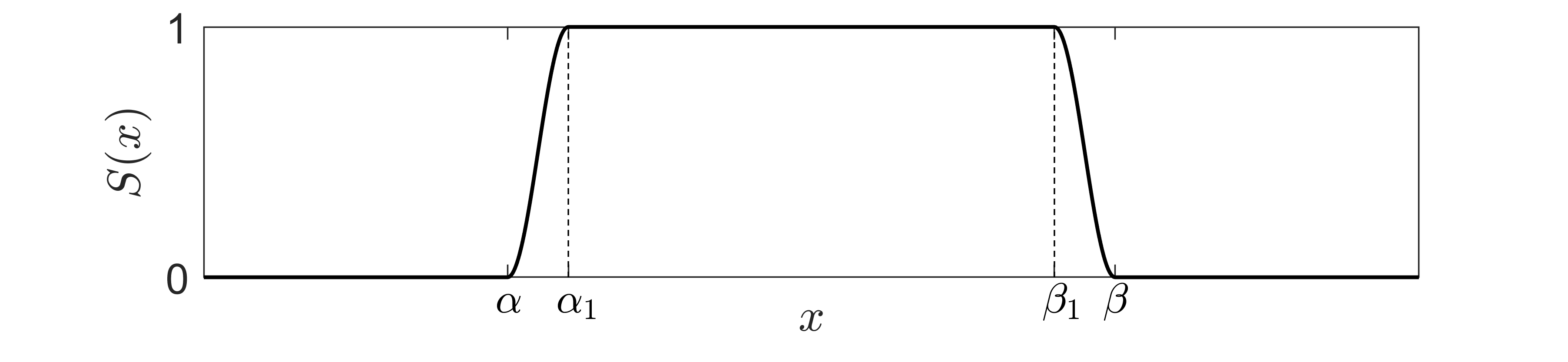
Figure 1: The bump function $S(x)$

In order to estimate $\nu(t)$, Guignard and Grilli (2001) asserted the similarity between a breaking wave and a hydraulic jump, proposing the following strategy: assume that the instantaneous power dissipated by $P_{\text{surf}}$, defined as $\Pi_{\text{surf}}$, is of the same order as the instantaneous power dissipated by a hydraulic jump, $\Pi_{\text{h}}$. Then, $\Pi_{\text{surf}}$ may be expressed as

$$\Pi_{\text{surf}}=\nu_{0}\Pi_{\text{h}},$$ (3.13)

where $\nu_{0}$ is a positive calibration constant. Eq. (3.13) will then be used to calculate $\nu(t)$ at every time $t$. Therefore, $\Pi_{\text{surf}}$ and $\Pi_{\text{h}}$ have to be expressed in terms of known quantities and $\nu(t)$. $\Pi_{\text{surf}}$ is given by the integral

$$\Pi_{\text{surf}} =\int P_{\text{surf}}\,G[\eta,h]\psi\,\sqrt{(\partial_{x}\eta)^{2}+1}dx,$$ (3.14)

which after substitution of Eq. (3.11) becomes

$$\Pi_{\text{surf}} =\nu(t)\int_{\Theta}S\,(G[\eta,h]\psi)^{2}\,\sqrt{(\partial_{x}\eta)^{2}+1}dx.$$ (3.15)

For the calculation of $\Pi_{\text{h}}$, Guignard and Grilli (2001) proposed the following formula

$$\Pi_{\text{h}}=g\,c\,d\,\frac{H_{\text{w}}^{3}}{4h_{c}h_{l}},$$ (3.16)

where $c$ is the phase speed, $d$ is the depth below the point of maximum front slope, $H_{\text{w}}(t)=\eta(x_{c},t)-\eta(x_{l},t)$ is the wave height defined as the height between the crest and the previous trough, $h_{c}(t)=\eta(x_{c},t)+h(x_{c})$ is the depth below the crest and $h_{t}=\eta(x_{l},t)+h(x_{l})$ is the depth below the trough (see Figure 2).

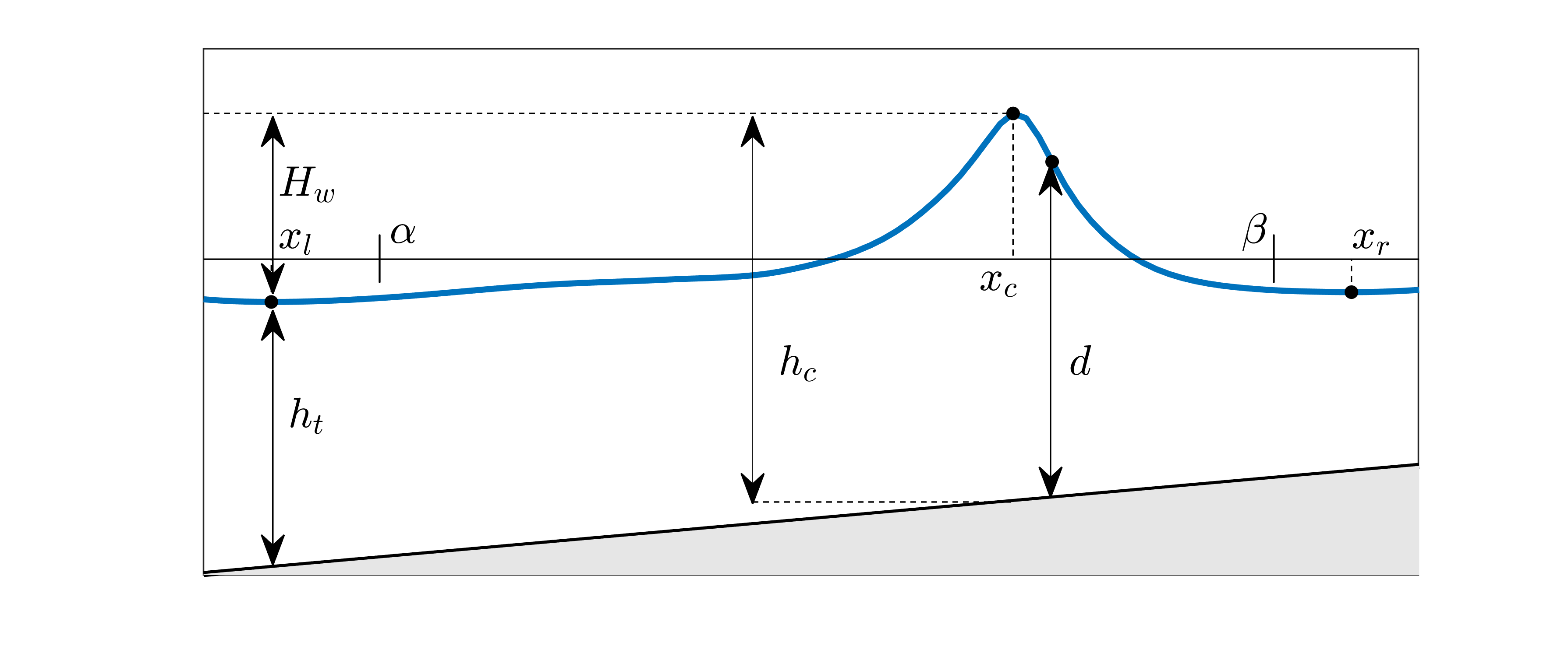
Figure 2: Geometric parameters used in the EHJ model.

The breaking initiation and termination criterion are the same as in the EVM approach. Concerning the breaking region $\Theta$, two different possibilities will be examined: (i) the region proposed by Guignard and Grilli (2001) in which the breaking region extends from the crest to two points $x=\alpha$ and $x=\beta$ on each side of the crest (see Figure 2):

$$\Theta:=[\alpha,\beta]=\left\{x\in[x_{l},x_{r}]:\left|\frac{\partial_{n}\Phi}{\max\partial_{n}\Phi}\right|>\varepsilon\quad\text{and}\quad\left|\frac{\partial_{n}\Phi}{\min\partial_{n}\Phi}\right|>\varepsilon\right\},$$ (3.17)

where $\partial_{n}\Phi$ is the normal velocity on the free surface ($\partial_{n}\Phi=G[\eta,h]\psi$), $\max\partial_{n}\Phi$ (resp. $\min\partial_{n}\Phi$) is the maximum (resp. minimum) of $\partial_{n}\Phi$ in the interval $[x_{l},x_{r}]$, and $\varepsilon$ is a small threshold value ($\varepsilon=10^{-4}$ in this work), and (ii) a breaking region covering only the front face of the wave, spanning from the breaking crest to the following trough, $\Theta=[x_{c},x_{r}]$, as in the EVM. The above two options will be refereed to as EHJ and EHJ_f, respectively. Note that the requirement that $d\mathcal{H}/dt$ is negative is not affected by the extent of the breaking region $\Theta$.

4 Numerical implementation

4.1 Hamiltonian Coupled-Mode Theory

The numerical implementation of Eqs. (3.1) is performed by using the Hamiltonian Coupled-Mode Theory (HCMT) (Athanassoulis and Papoutsellis, 2015; Papoutsellis and Athanassoulis, 2017), which is briefly described below. In this approach, the unknown velocity potential $\Phi(x,z,t)$ is expressed as a rapidly convergent series expansion in terms of unknown horizontal functions $\{\varphi_{n}\}_{n=-2}^{\infty}=\{\varphi_{n}(x,t)\}_{n=-2}^{\infty}$ and prescribed vertical basis functions $\{Z_{n}\}_{n=-2}^{\infty}=\{Z_{n}(z;\eta(x,t),h(x))\}_{n=-2}^{\infty}$:

$$\Phi(x,z,t)=\sum\limits_{n=-2}^{\infty}\varphi_{n}(x,t)Z_{n}(z;\eta(x,t),h(x)).$$ (4.1)

The exact form of $\{Z_{n}\}_{n=-2}^{\infty}$ is given in B by Eqs. (B.1a), (B.1b), (B.1c) and (B.1d). More information about the above expansion and its convergence can be found in Athanassoulis and Papoutsellis (2017). Using expansion (4.1) and restricting the horizontal computational domain to the interval $[a,b]$, Eqs. (3.1) take the form (Papoutsellis and Athanassoulis, 2017)

$$\partial_{{\kern 1.0pt}t}\eta =-(\partial_{x}\eta)(\partial_{x}\psi)+({\kern 1.0pt}|\partial_{x}\eta{\kern 1.0pt}|^{2}+1)\left(h_{0}^{-1}{\kern 1.0pt}\mathcal{F}[\eta,h]\psi+\mu_{{\kern 1.0pt}0}\psi\right),$$ (4.2a)

$$\partial_{{\kern 1.0pt}t}\psi =-g{\kern 1.0pt}\eta-\frac{1}{2}(\partial_{x}\psi)^{2}+\frac{1}{2}({\kern 1.0pt}|\partial_{x}\eta{\kern 1.0pt}|^{2}+1)\left(h_{0}^{-1}{\kern 1.0pt}\mathcal{F}[\eta,h]\psi+\mu_{0}\psi\right)^{2}+P_{\text{surf}},$$ (4.2b)

where $\mathcal{F}[\eta,h]\psi=\varphi_{-2}(x,{\kern 1.0pt}t)$ is the first element of the sequence that solves the following coupled-mode system

$$\sum_{n=-2}^{\infty}\left(A_{mn}\partial_{x}^{2}+B_{mn}\partial_{x}+C_{mn}\right)\varphi_{n} =0,\quad m\geq-2,\quad a<x<b,$$ (4.3a)

$$\sum_{n=-2}^{\infty}{\kern 1.0pt}\varphi_{n} =\psi,\quad a<x<b,$$ (4.3b)

$$\sum_{n=-2}^{\infty}\left(A_{mn}\partial_{x}+\frac{1}{2}B_{mn}\right)\varphi_{n} =g_{m},\quad m\geq-2,\quad x=a,$$ (4.3c)

$$\sum_{n=-2}^{\infty}\left(A_{mn}\partial_{x}+\frac{1}{2}B_{mn}\right)\varphi_{n} =0,\quad m\geq-2,\quad x=b,$$ (4.3d)

with

$$A_{mn} =\int_{-h}^{\eta}Z_{n}Z_{m}dz=A_{nm},$$ (4.4a)

$$B_{mn} =2\int_{-h}^{\eta}\partial_{x}Z_{n}Z_{m}dz+\partial_{x}h\big{[}Z_{n}Z_{m}\big{]}_{z=-h},$$ (4.4b)

$$C_{mn} =\int_{-h}^{\eta}\Delta Z_{n}Z_{m}dz+\partial_{x}h\big{[}\partial_{x}Z_{n}Z_{m}\big{]}_{z=-h}-\big{[}\partial_{z}Z_{n}Z_{m}\big{]}_{z=-h}.$$ (4.4c)

The $(x,t)-$dependent matrix coefficients $A_{mn}=A_{mn}(\eta,h)$, $B_{mn}=B_{mn}(\eta,h)$ and $C_{mn}=C_{mn}(\eta,h)$ are calculated analytically in terms of $\eta(x,t)$, $h(x)$ and the numerical parameters $h_{0}$, $\mu_{0}$ that are involved in the definition of $\{Z_{n}\}_{n=-2}^{\infty}$ (Papoutsellis et al., 2018, Section 4). The boundary condition expressed by Eq. (4.3c) forces the horizontal fluid velocity at the vertical section $x=a$ to match

$$g_{m}(t)=\int_{h(a)}^{\eta(a,t)}\partial_{x}\Phi(a,z,t)Z_{m}(z)dz,$$ (4.5)

and it is used to generate incident waves (Sections 5.2 and 5.3). If $g_{m}=0$, the boundary condition Eq. (4.3c) represents a reflecting wall, such as in Eq. (4.3d). As opposed to the standard definition of the DtN operator $G[\eta,h]\psi$ of the Laplace problem in the entire fluid domain, $\mathcal{F}[\eta,h]\psi$ is determined at every time $t$, by solving a system of differential equations in the fixed horizontal domain $[a,b]$. In fact, as shown in Athanassoulis and Papoutsellis (2017), $G[\eta,h]\psi$ and $\mathcal{F}[\eta,h]\psi$ are related by the following formula

$${\rm{\mathcal{G}}}[\eta,h]\psi=-(\partial_{x}\eta)(\partial_{x}\psi)+\left((\partial_{x}\eta)^{2}+1\right)\left(h_{0}^{-1}\mathcal{F}[\eta,h]\psi+\mu_{0}\psi\right).$$ (4.6)

4.2 Computation of the DtN Operator

In order to compute the DtN operator, the coupled-mode system, Eqs. (4.3a)-(4.3d), is truncated at a finite order $M$. Horizontal spatial gradients are approximated using a fourth-order finite-difference method applied on a grid $x_{i}$, $i=1,...,N_{X}$, of uniform spacing $\delta x$. First and second-order horizontal derivatives of $\varphi_{n}$, $n=-2,...,M$ are approximated by using the formulae (C.1) and (C.2) given in C, and a linear system of algebraic equations is formed of the local values $\varphi_{n}^{i}$, $n=1,...,N_{\text{tot}}=M+3$, $i=1,...,N_{X}$ (see Papoutsellis et al. (2018, Appendix D)). The local values $\mathcal{F}[\eta,h]\psi$ are then recovered and used in Eq. (4.6) for the computation of the DtN operator. A detailed study of the convergence and accuracy of the above scheme with respect to $N_{\text{tot}}$ can be found in Athanassoulis and Papoutsellis (2017).

4.3 Computation of $P_{\text{surf}}$

4.3.1 Eddy Viscocity Model

With $F$ given by Eq. (3.7), Eq. (3.6) is written

$$\begin{aligned} \partial_{x}P_{\text{surf}}&=\delta^{2}B(\partial_{t}\eta)\frac{1}{H}\partial_{x}\left(H\,(G[\eta,h]\psi)^{2}\right)\\ &=\delta^{2}B(\partial_{t}\eta)\left[\frac{\partial_{x}H}{H}(G[\eta,h]\psi)^{2}+2\,G[\eta,h]\psi\,\partial_{x}(G[\eta,h]\psi)\right].\end{aligned}$$ (4.7)

Differentiating Eq. (4.7) yields a second-order differential equation

$$\partial_{x}^{2}P_{\text{surf}}=\delta^{2}B(\partial_{t}\eta)\left[\left(\frac{\partial_{x}^{2}H}{H}-\frac{(\partial_{x}H)^{2}}{H^{2}}\right)\,(G[\eta,h]\psi)^{2}+2\,(\partial_{x}(G[\eta,h]\psi))^{2}\right.\\ \left.+2\,G[\eta,h]\psi\left(\frac{\partial_{x}H}{H}\partial_{x}(G[\eta,h]\psi)+\partial_{x}^{2}(G[\eta,h]\psi)\right)\right].$$ (4.8)

When Eq. (4.8) is combined with the boundary conditions

$$P_{\text{surf}}(x_{c})=P_{\text{surf}}(x_{r})=0,$$ (4.9)

which ensure that $P_{\text{surf}}$ vanishes at the endpoints of the breaking region, a solvable boundary value problem is defined for $P_{\text{surf}}$. At every time $t$, Eqs. (4.8) and (4.9) are solved using a fourth-order finite-difference method in accordance with the numerical scheme used for the computation of the DtN operator. The derivatives appearing in the right hand side of Eq. (4.8) are calculated using formulae (C.1) and (C.2).

4.3.2 Effective Hydraulic Jump

The geometrical characteristics appearing in Eq. (3.16) are easily calculated during the wave evolution. However, the estimation of the phase speed $c$ is not straightforward since breaking waves do not have a permanent form. Therefore, to calculate the phase speed, the spatial Hilbert transform technique proposed by Kurnia and van Groesen (2014) is used. The integral in Eq. (3.15) is calculated using the trapezoidal rule.

4.4 Time stepping scheme

Having established methods to compute $\mathcal{F}[\eta,h]\psi$ (or $G[\eta,h]\psi$) and $P_{\text{surf}}$, the local values of $(G[\eta,h]\psi)^{i}$ and $P_{\text{surf}}^{i}$, $i=1,...,N_{X}$, can be used to step forward in time Eqs. (4.2). The derivatives appearing on the right hand sides of Eqs. (4.2) are approximated by the finite-difference formulae (C.1). In the case of an initial value problem, the initial conditions $\eta(x,0)$ and $\psi(x,0)$ are propagated using the classical fourth-order four-step Runge-Kutta method. For wave problems involving incident wave conditions, Eqs. (4.2) are supplemented by the following expression:

$$\partial_{t}U=N({\kern 1.0pt}U)+L(U)$$ (4.10)

where $U=(\eta,\psi)^{{\rm T}}$, $N(U)$ is the vector function defined by the right-hand sides of Eqs. (4.2) and $L(U)=c_{a}(U-U_{\text{in}})+c_{b}(0\,,G[\eta,h]\psi)^{{\rm T}}$. Functions $c_{a}(x)$ and $c_{b}(x)$ are polynomials supported in small regions (sponge layers) before the boundaries $x=a$ and $x=b$ (one and two wavelengths of the incident wave for $c_{a}$ and $c_{b}$, respectively). The first term of $L(U)$ is used for wave generation and absorption: $U_{\text{in}}$ denotes the desired incident wave condition, such that $U_{\text{in}}=D(t)(\eta_{\text{in}},\psi_{\text{in}})^{{\rm T}}$, where $(\eta_{\text{in}},\psi_{\text{in}})^{{\rm T}}$ is a steady travelling wave solution of system (4.2) (Papoutsellis, 2016, Chapter 6), and $D(t)$ is a smooth function ranging from 0 to 1 in a time interval of typically 3-5 incident wave periods. The second term implies a pressure-type wave absorption.

A routine is applied at each time step to evaluate the breaking criterion at every node. The wave characteristics (crest and trough locations) are saved at every time step and are passed to the following time step in order to enable tracking of breaking and non-breaking waves. The above scheme requires four solutions of the linear discretized system (4.3) and one application of the wave tracking algorithm per time step. It is implemented by using Matlab^® on an IntelCore i5-8300H, 2.30 GHz. The CPU time needed for the wave tracking algorithm is a small percentage of the total CPU time per time step. Depending on the discretization used (number of modes $N_{tot}$ and number of grid points $N_{X}$) this percentage ranges from 5-10 % of the total CPU time per time step. The difference in CPU time between the two proposed methods is insignificant. For the three test cases studied in this paper, the total CPU times per time step are approximately 0.11 sec (Section 5.1), 0.1 sec (Section 5.2 ), and 0.23 sec (Section 5.3).

5 Application and validation cases

In this section, the proposed numerical scheme is implemented for the simulation of breaking waves. The optimal set of numerical and breaking parameters is chosen after performing a series of numerical simulations to obtain a good compromise between numerical convergence and the agreement with experimental measurements. To choose the optimal number of total modes $N_{\text{tot}}$, a series of simulations are performed by increasing $N_{\text{tot}}$ (starting with $N_{\text{tot}}=4$) until numerical convergence of the free-surface elevation is achieved. Before presenting the simulation results, the calibration process of both breaking models is described. For a given test case, the parameters controlling the initiation ($\gamma_{\text{I}}$) and termination ($\gamma_{\text{F}}$) of wave breaking are the same for each wave breaking approach. The value of these two parameters depends on the configuration (e.g. bathymetry) and type of wave breaking studied. The EVM approach has two free parameters, namely $\delta$ and $T^{*}$, which were set to $\delta=1.5$ and $T^{*}=5\sqrt{h/g}$ in all cases. The EHJ approach has three free parameters: the coefficient $\nu_{0}$, the threshold value $\varepsilon$ that determines the length of the breaking region, and the factor $\sigma$ appearing in the definition of the smooth function $S(x)$. The simulation results were not very sensitive to the value of the two latter parameters, which were thus set to $\varepsilon=10^{-4}$ and $\sigma=0.1$ in all simulations. For the coefficient $\nu_{0}$, the value $\nu_{0}=1.6$ was chosen in the case of a sloping bottom and $\nu_{0}=1.0$ in the case of a flat bottom. These parameters remained identical for the EHJ and EHJ_f simulations.

5.1 Dispersive shock waves

In this section, the propagation of two breaking dispersive shock waves (DSW) are simulated over a flat bottom. The first test aims to verify the dissipation and conservation properties of the proposed methods, and the second test reproduces a laboratory experiment.

5.1.1 Momentum conservation and energy dissipation

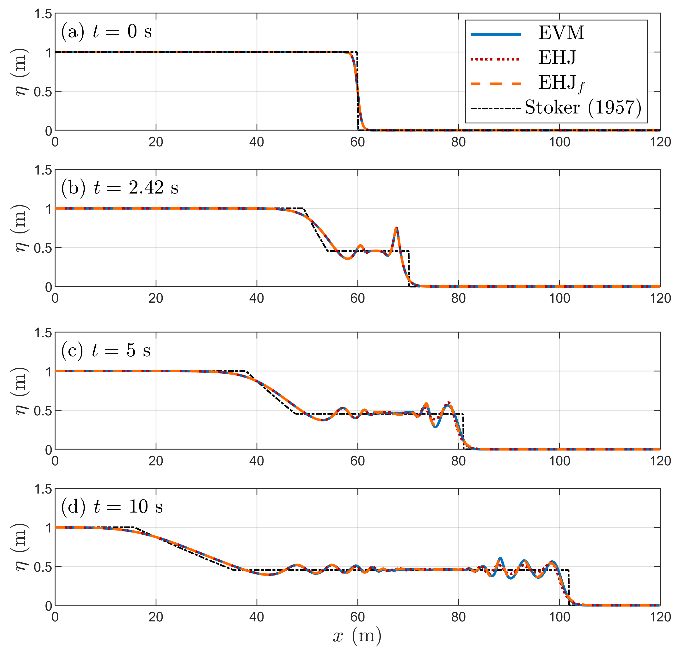
Figure 3: Snapshots of the free-surface elevation for the case of a breaking DSW.

Two important questions are whether the EHJ method, constructed by requiring energy dissipation, conserves momentum, and whether the EVM, constructed by requiring momentum conservation, dissipates energy. In order to answer these questions, a test case is presented showing the evolution of two counter-propagating DSWs created after a dam break (see e.g. Mitsotakis et al., 2017). The horizontal domain extends from -120 to 120 m, and the initial hump of water, centered at $x=0$, is given by

$$\eta(x,0)=\frac{1}{2}(H_{2}-H_{1})\left(1+\tanh\left(\frac{\lambda-|x|}{s}\right)\right),$$ (5.1)

with $H_{1}=1$ m, $H_{2}=2$ m and $\lambda=60$ m. The parameter $s$ controls the initial surface slope and is chosen as $s=0.8$ m. The depth measured from $z=0$ is $h=1$ m. The initial free-surface potential is $\psi(x,0)=0$, which implies that the initial fluid velocity and momentum are zero. The simulation is performed using $N_{\text{tot}}=5$ vertical functions and a spatio-temporal discretization $\delta x=0.1$ m, $\delta t=0.01$ s. Wave breaking is initiated using $\gamma_{I}=0.6$. The value $\gamma_{\text{F}}=0.2$ is used for the termination criterion, but it is not reached during the duration of the simulation. For the EVM, $\delta=1.5$ and for the EHJ, $\nu_{0}=1$. Snapshots of the simulated free-surface elevations are shown in Figure 3 for the right half of the (symmetric) computational domain. For reference, the analytical solution of the NSW equations with a piecewise constant initial condition (Riemann problem) is also plotted (Stoker (1957), Section 4.1.1); see also (Delestre et al. (2013), Section 4.1.1). In the simulations, breaking occurs at $t=2.42$ s, and only the first counter-propagating waves break. The EVM and EHJ_f show nearly identical results while EHJ predicts slightly smaller wave heights for the dispersive tails following the breaking fronts. When comparing to the NSW solution, it is observed that the neglect of dispersive effects in the NSW equations leads to an inadequate description of the DSW’s surface elevation.

Figure 4 shows the ratio $\mathcal{H}(t)/\mathcal{H}_{0}$ (where $\mathcal{H}_{0}$ is the initial total energy), the logarithm of the relative error of the mass, $\mathcal{E}\left[\mathcal{M}(t)\right]=\left|\mathcal{M}(t)/\mathcal{M}_{0}-1\right|$ and the logarithm of the momentum $\mathcal{I}(t)$. Both methods dissipate energy and conserve momentum. Mass is also well conserved in the simulations. The EHJ and EHJ_f methods dissipate energy at the same constant rate. This is expected since, in this method, the extent of the breaking region does not affect the amount of dissipated energy. In the EVM approach, the dissipation rate increases gradually during a transition period after which it remains constant.

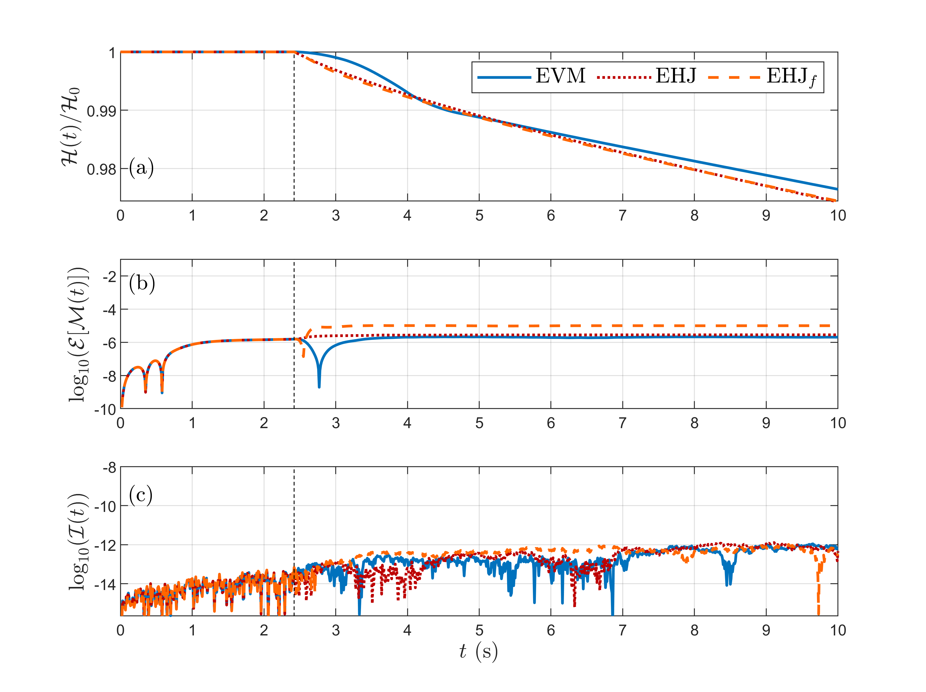
Figure 4: Evolution of (a) the Hamiltonian, (b) the logarithm of the relative error on the mass, and (c) the logarithm of the horizontal momentum for the simulation of two counter-propagating breaking DSWs. The vertical dashed line indicates the initiation of breaking.

5.1.2 Dam-break experiment of do Carmo et al. (1993)

Next, the dam-break experiment of do Carmo et al. (1993) is simulated. In a rectangular wave tank, two different volumes of water of heights $H_{2}=0.099$ m and $H_{1}=0.051$ m are separated by a gate or dam. Upon the sudden removal of the dam, a dispersive shock wave propagates downstream. As shown in do Carmo et al. (2019), both wave breaking and strong dispersive effects play an important role in this experiment. For the simulation, the removal of the dam is modeled by considering an initial free-surface elevation of the form

$$\eta(x,0)=\frac{1}{2}(H_{2}-H_{1})\left(1-\tanh\left(\frac{x_{0}-x}{s}\right)\right),$$ (5.2)

where $x_{0}=3.8$ m is the location of the gate, and $s=0.1$ m (see Figure 5 (a)). Computations are performed by using $\delta x=0.01$ m, $\delta t=0.01$ s and $N_{\text{tot}}=5$ vertical functions. Wave breaking is initiated with $\gamma_{\text{I}}=0.6$. Note that the value $\gamma_{\text{F}}=0.3$ used for the termination criterion was not reached during the duration of the simulation.

Figure 5 compares the computed free-surface elevation with the experimental measurements at three locations. Note that a time shift of 0.2 s was needed to match the results at the first station, and this time shift is therefore applied at all stations. As noted in do Carmo et al. (2018), this lag is may be explained by the physical difference between the initial condition used in the simulations and the removal of the dam in the experiment of do Carmo et al. (1993). All computations agree well with the experiments at the first station (Figure 5(b)) but overestimate the height of the front wave at the next two stations (Figures 5(c) and (d)). At these two stations, EHJ underestimates the wave heights of the waves following the breaking front, while EVM and EHJ_f perform better. At the last station, a small phase shift is observed for all methods (Figure 5(d)), which likely can be attributed to the difference between the initialization of the experiment and the simulation.

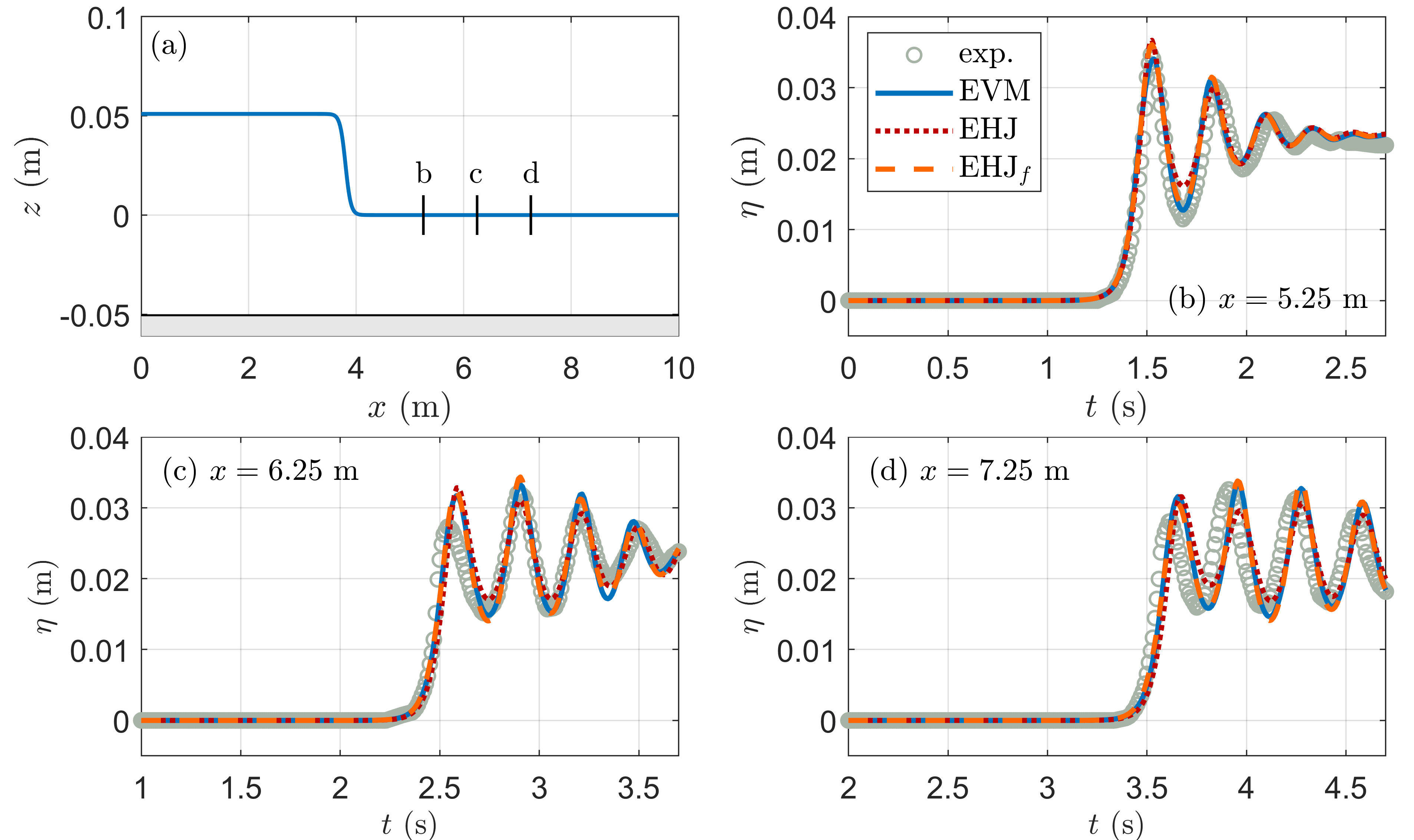
Figure 5: (a) Initial configuration for the experiment of do Carmo et al. (1993). Vertical lines mark the locations of the measuring gauges. (b,c,d) Comparison of computed free surface elevation with experimental measurements.

5.2 Breaking of shoaling regular waves on a sloping beach (Ting and Kirby, 1994)

In this section, the spilling breaking experiment of Ting and Kirby (1994) is considered. Incident waves of wave height $H=0.125$ m and period $T=2.0$ s (wavelength $L=3.85$ m) are generated in constant depth $h_{0}=0.4$ m and propagate towards a plane beach of slope 1/35. Non-synchronised measurements of the free-surface elevation, as well as the corresponding mean crest, trough, and water levels are available at 21 locations along the wave tank. Due to the absence of a moving shoreline in the current numerical model, the original geometry is modified in the simulation: after reaching a minimum depth $h=0.0434$ m, an absorbing sponge layer is applied, and in this zone the bathymetry deepens again with a slope 1/10 until $h=0.2915$ m (Figure 6). Simulations are performed using $N_{\text{tot}}=4$ vertical functions, a spatial grid with $\delta x=L/150=0.0257$ m, and a time step $\delta t=T/200=0.01$ s. Breaking is initiated with $\gamma_{\text{I}}=0.6$ and terminated with $\gamma_{\text{F}}=0.1$. Note that breaking terminates inside the sponge layer. The variant EHJ_f of EHJ, where only the wave front is considered as the breaking region, rapidly becomes unstable, and the simulations could not be completed.

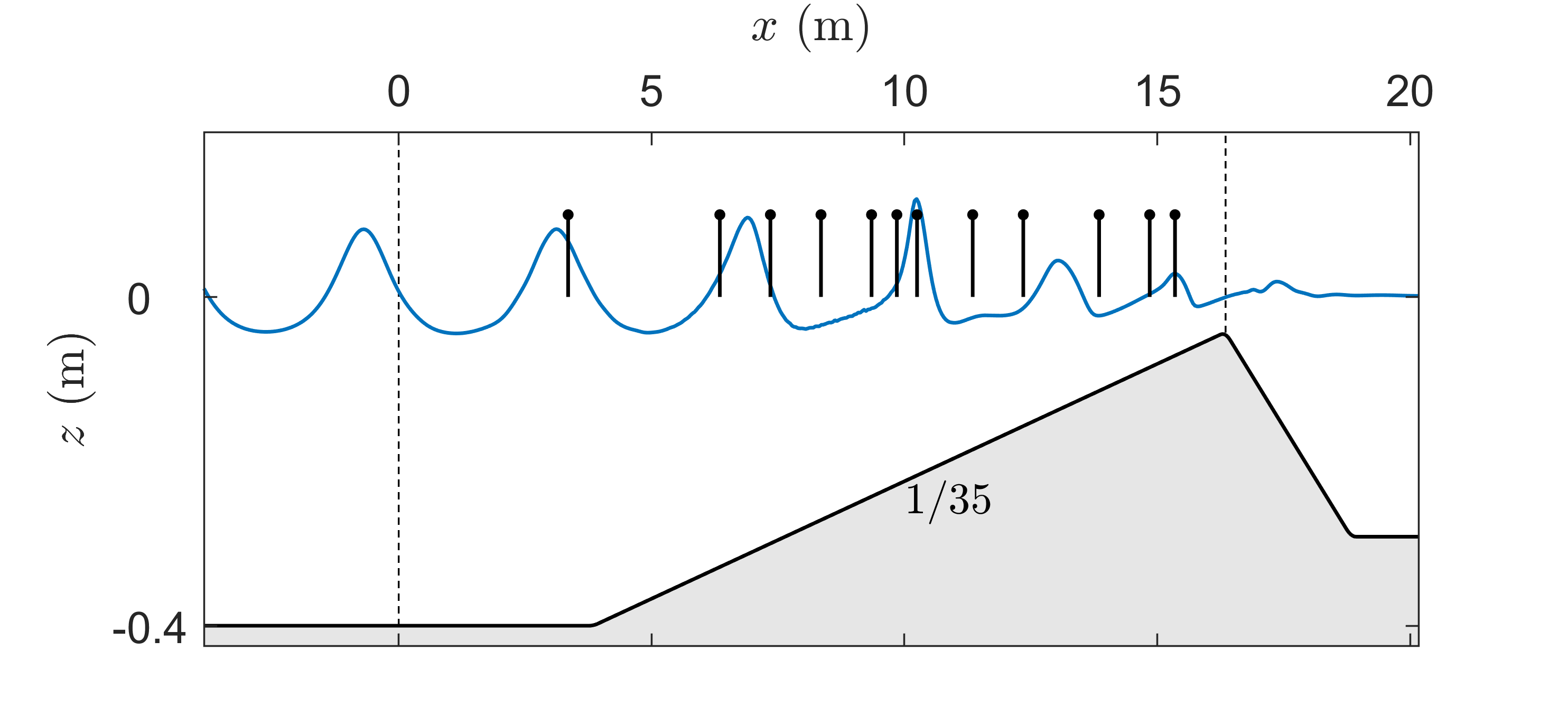
Figure 6: Bathymetry used in the simulations to represent the experiment of Ting and Kirby (1994). Vertical lines correspond to the wave gauge locations. Sponge layers are indicated by the vertical dashed lines.

In Figure 7, the computed free-surface elevation is compared with the experimental measurements at 12 locations spanning the shoaling and surf zones (Figure 6). The computed and measured free-surface elevation profiles agree well up to $x=9.85$ m. In the vicinity of the breaking point, around $x=10.25$ m, the EVM slightly underestimates the wave height, while the EHJ method significantly underestimates the wave height. Some discrepancies in the wave shape are also noticeable at the last four stations for both wave breaking approaches.

The maximum and minimum of the spatial variations of the time-averaged surface elevation levels are reproduced well (Figure 8). Breaking in the simulations occurs slightly earlier ($x=9.7$ m) than observed in the experiments ($x=10.25$ m). This likely explains why the simulations underestimate the wave heights at $x=10.25$ m in Figure 7. Also at this location, the more significant underestimation of the wave height by the EHJ method is explained by the abrupt application of wave breaking energy dissipation, while in the EVM it is applied smoothly in time. Concerning the prediction of set-up, both simulations agree well with the laboratory data before the breaking point, but underestimate the increase in the mean water level in the surf zone (Figure 8). This trend is also visible in other modeling approaches (Cienfuegos et al., 2010; Tissier et al., 2012).

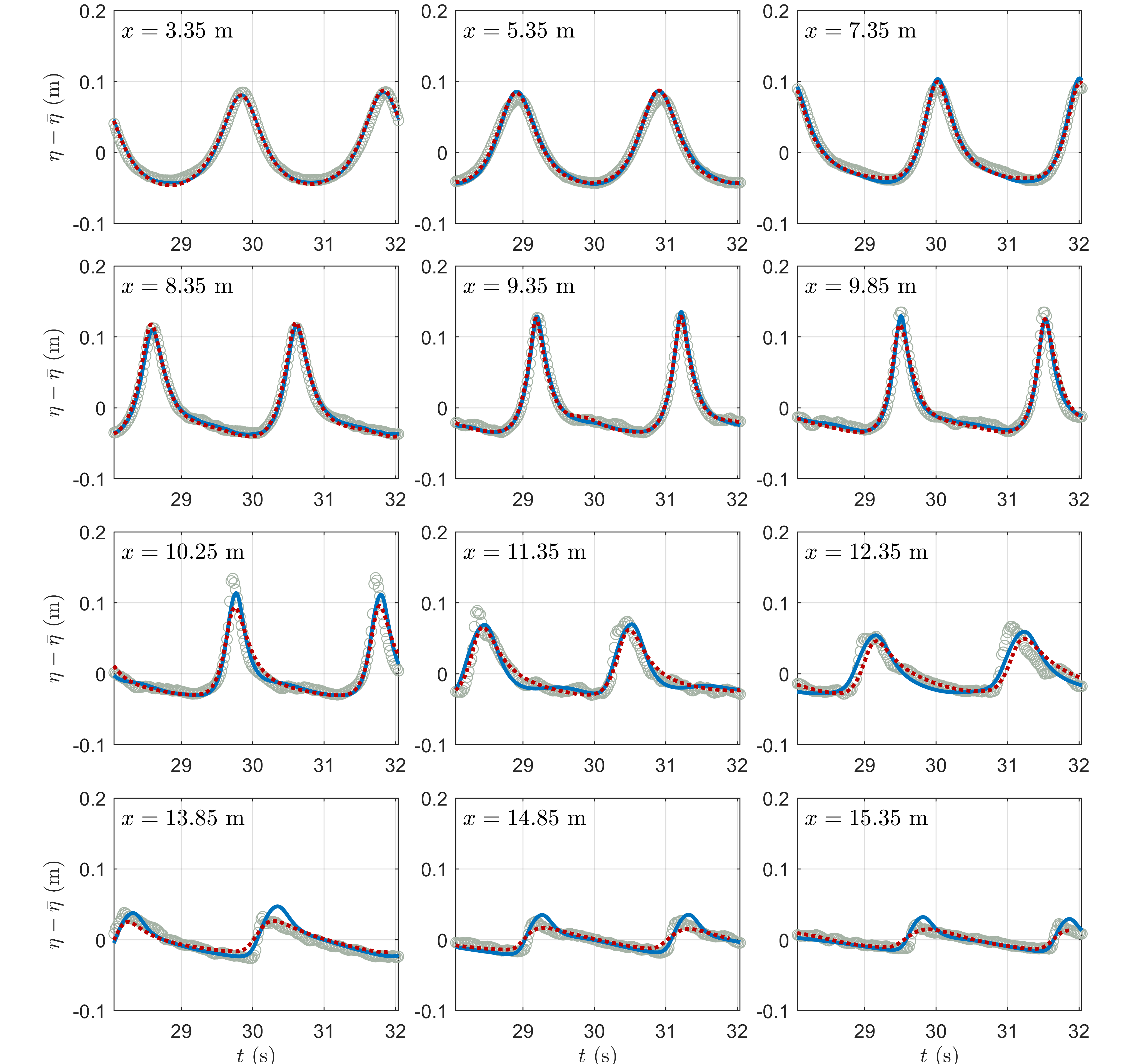
Figure 7: Comparison of experimental data (circles) and the simulated EVM (plain lines) and EHJ (dotted lines) time series of the free surface elevation at the locations shown in Figure 6 for the case of shoaling and spilling breaking of regular waves propagating over a mildly sloping beach (Ting and Kirby, 1994). Breaking begins around $x=10.25$ m

.

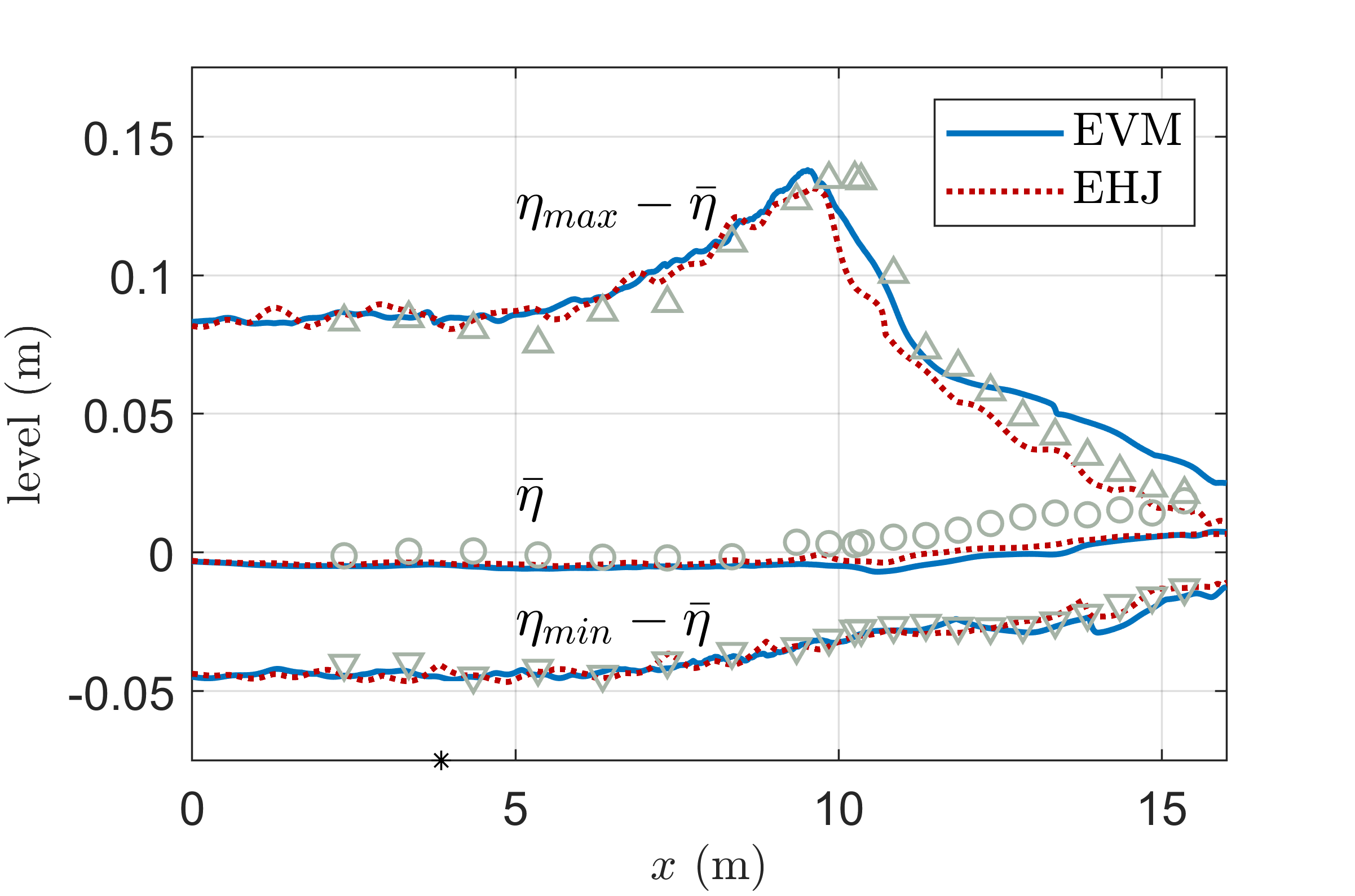
Figure 8: Simulated spatial variation of the Mean Water Level (MWL) $\bar{\eta}$, maximum elevation relative to MWL $\eta_{max}-\bar{\eta}$, and minimum elevation relative to MWL $\eta_{min}-\bar{\eta}$, for the experiment of Ting and Kirby (1994). The asterisk indicates the toe of the beach. Numerical results are averaged over $10T$ sec.

To further assess the ability of the proposed models to reproduce accurately the nonlinear wave shape, the skewness Sk and asymmetry As of the surface elevation are calculated following Kennedy et al. (2000):

$$\text{Sk}=\frac{\left<(\eta-\bar{\eta})^{3}\right>}{\left<(\eta-\bar{\eta})^{2}\right>^{3/2}},\qquad\text{As}=\frac{\left<\left[\,\mathbb{H}(\eta-\bar{\eta})\,\right]^{3}\right>}{\left<(\eta-\bar{\eta})^{2}\right>^{3/2}},$$

where $\left<\,\right>$ is the time-averaging operator, $\bar{\eta}=\left<\eta\right>$ and $\mathbb{H}$ denotes the Hilbert transform. Figure 9 shows a comparison of the measured and computed spatial variation of Sk and -As. For the EVM, the skewness Sk is reproduced accurately in the shoaling region and in a portion of the surf zone spanning from $x=11.35$ to 13.85 m. Differences appear in a small region after the breaking point and in the last 2-3 meters of the inner surf zone. Concerning the wave asymmetry As, the EVM simulation results agree well with the experimental measurements until the breaking point, after which it is underestimated. Similar trends are also present in computations using a BT model with Kennedy’s eddy viscosity approach (Cienfuegos et al., 2010, Figures 2,4) and in computations using a GN model with the Hybrid approach (Tissier et al., 2012, Figure 7). Using the EHJ approach, the wave skewness is reproduced well except for a small region around the breaking point. The simulated wave asymmetry also agrees well with the experimental measurements in the shoaling region but presents some differences after breaking begins. In comparison to the EVM, the EHJ method generally predicts smaller values of Sk, and first smaller and then ($x\geq 13.5$ m) larger values of -As in the region after the breaking point.

On the basis of the above results, both methods predict accurately the wave height evolution during the shoaling/breaking process in comparison with BTM approaches (see e.g Tissier et al. (2012), Figure 7 (a)) or the Reynold Averaged Navier-Stokes approach (see Derakhti et al. (2016), Figure 2(a)). Differences in the wave shape in the surf zone do exist and, as mentioned earlier, this drawback is also present in the original eddy viscosity approach (see the discussion in Cienfuegos et al. (2010)) and the Hybrid approach applied in BTMs (see e.g. Tissier et al. (2012), Figure 7 (c)). It is observed that both EVM and EHJ methods induce a dissipation rate that is not optimal for the spilling breaking case. Controlling the dissipation rate by considering breaking regions of arbitrary length may be one possible option to investigate. Note, however, this would introduce at least one more free parameter (breaking region length) in the resulting breaking model.

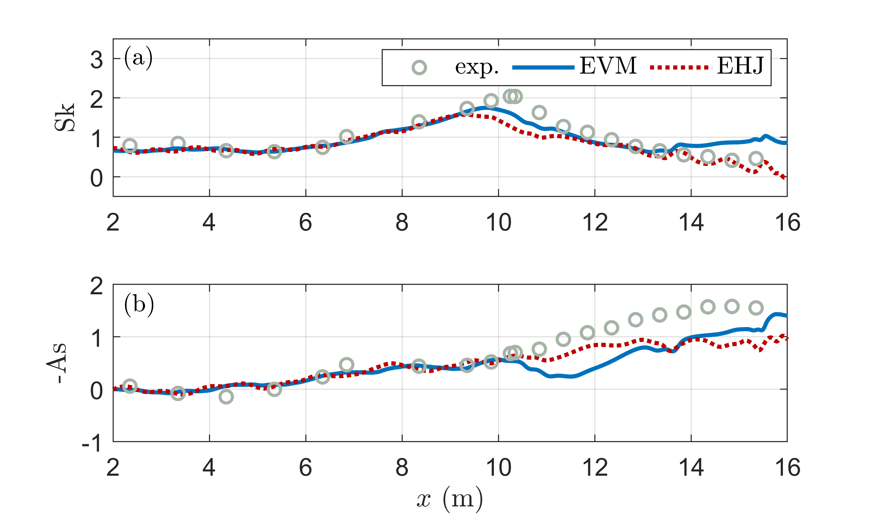
Figure 9: Spatial variation of the (a) wave skewness Sk and (b) wave asymmetry As for the experiment of Ting and Kirby (1994). Numerical results averaged over $10T$ sec.

5.3 Regular waves breaking over a bar (Beji and Battjes, 1993)

Beji and Battjes (1993) investigated the transformation of periodic waves propagating over a submerged trapezoidal bar (Figure 10). In the experiments, the incident wave train shoals along the front face of the bar, and bound harmonics are amplified. Plunging breaking occurs over the top of the bar, and then higher harmonics are released on the lee side of the bar, creating a strongly dispersive wave form. The case simulated here corresponds to a long wave generated in a constant depth $h_{0}=0.4$ m with period $T=2.5$ s ($f=0.4$ Hz, wavelength $L=4.8$ m) and wave height $H=0.054$ m. For the simulations, the spatio-temporal discretization is $\delta x=L/180=0.0267$ m, $\delta t=T/180=0.014$ s, and $N_{\text{tot}}=6$ vertical functions are used to compute the DtN operator. Breaking is initiated with $\gamma_{\text{I}}=0.3$ and terminated with $\gamma_{\text{F}}=0.1$.

Figure 11 shows snapshots of the computed free surface elevation using the EVM and EHJ. Incident waves start breaking before the top of the bar, at $x=11.57$ m. In the case of the EVM, the waves continue breaking until reaching $x=14.4$ m, after passing the top edge of the bar. During this phase, the next incoming wave starts breaking, and two breaking fronts exist simultaneously. This is also observed when using the EHJ_f (not shown here) and agrees with the simulation results shown by Kazolea et al. (2014). However, when using the EHJ, wave breaking stops sooner, at $x=13.76$ m, and only a single breaking wave exists at any moment in time during the simulation.

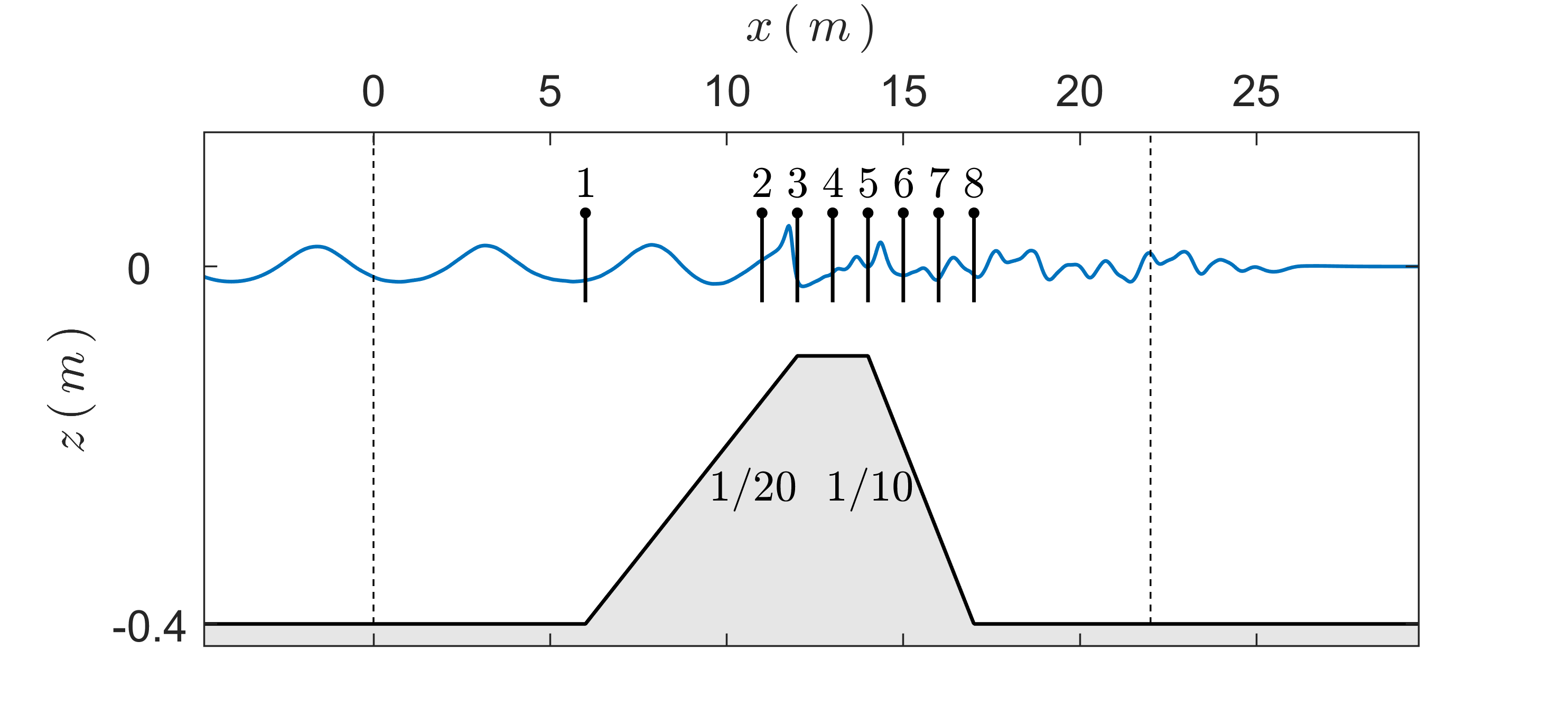
Figure 10: Bathymetry in the experiment of Beji and Battjes (1993). Vertical lines indicate the locations of the wave gauges. Vertical dashed lines indicate the extent of the sponge layers.

The simulated time series of the free-surface elevation at the eight wave gauge locations are compared with the experimental measurements in Figure 12. Good agreement with the experimental measurements is obtained for all three simulation methods. Differences are visible only at stations #4 and #6, where EVM and EHJ_f capture the wave transformation processes slightly more accurately than EHJ.

Figure 13 shows the spatial variation of the significant wave height Hs (calculated as four times the standard deviation of the surface elevation), skewness Sk and asymmetry As (Eq. ($(5.3a,b)$)). These nonlinear wave characteristics are reproduced well when using the EVM. The EHJ underestimates Hs after breaking and provides a fair prediction of Sk and As. The EHJ_f reproduces well Hs and As but shows some differences in Sk after breaking.

Next, a spectral analysis of the computed and experimental time-series of the free-surface elevation is performed in order to assess the energy transfers between harmonics and the wave decomposition process (Figure 14). Before the breaking point (wave gauge #2, $x=11$ m) and for the next two stations, all three methods agree well with each other and with the experiment, capturing the energy transfer processes to higher harmonics, with the exception of a small underestimation of the second harmonic amplitude. Starting from wave gauge #5, the EVM and EHJ_f approaches produce similar results, accurately reproducing the wave decomposition process, while the EHJ approach underestimates the amplitude of the third harmonic.

Taking into account the complexity of the physical processes (e.g. violent air-water mixing during post breaking evolution), the EVM and EHJ_f reproduce well the free-surface effects. Using the EVM, differences are obtained for the wave skewness at wave gauge #6 and for the wave asymmetry at wave gauge #5. Differences for the EHJ_f approach are obtained for wave skewness at wave gauges #5 and #6 and for the asymmetry at wave gauge #5. Finally, it is important to note that, although a small phase error is obtained at the last two wave gauges where dispersive effects are most important, both methods reproduce accurately the wave skewness and asymmetry.

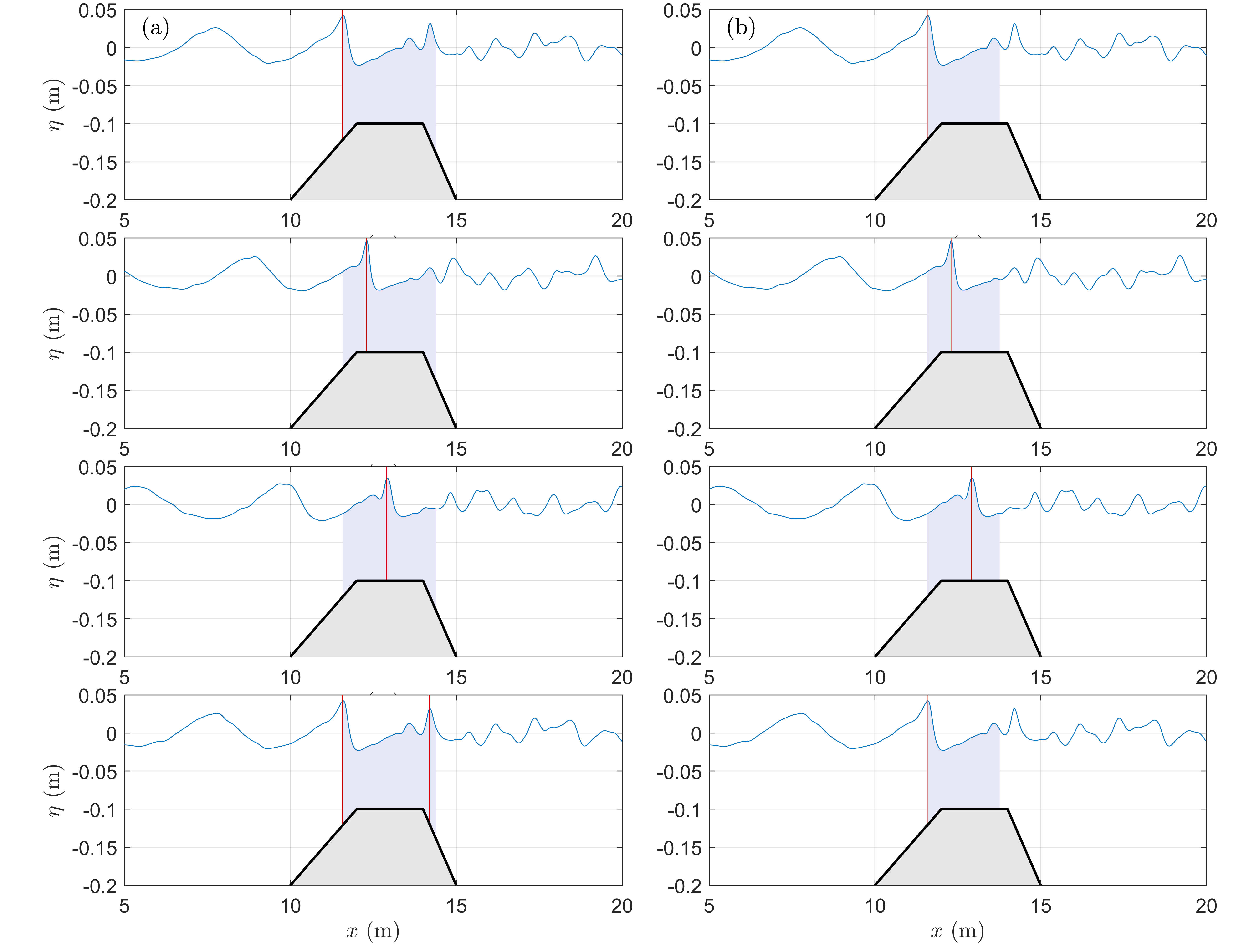
Figure 11: Snapshots of the simulated free-surface elevation for the experiment of Beji and Battjes (1993) using EVM (column (a)) and EHJ (column (b)). Vertical lines correspond to the crests of the breaking waves. The shaded area indicates the spatial extent of wave breaking in each simulation.

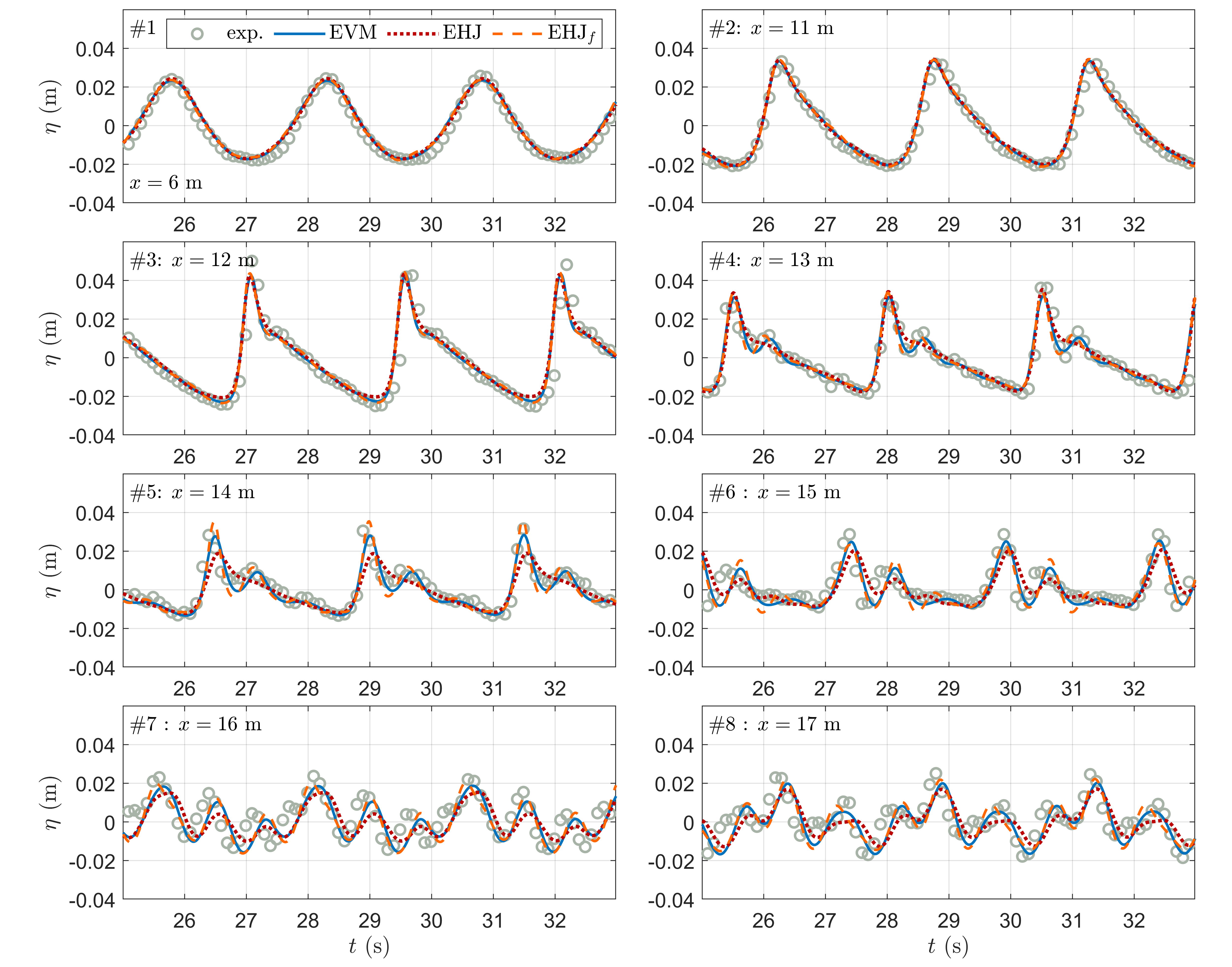
Figure 12: Comparison of experimental data (circles) and the EVM (plain lines), EHJ (dotted lines) and EHJ_f (dashed lines) simulation results. Free-surface elevation time series at locations #1-#8 for the transformation and plunging breaking of regular waves propagating over a submerged bar (Beji and Battjes, 1993).

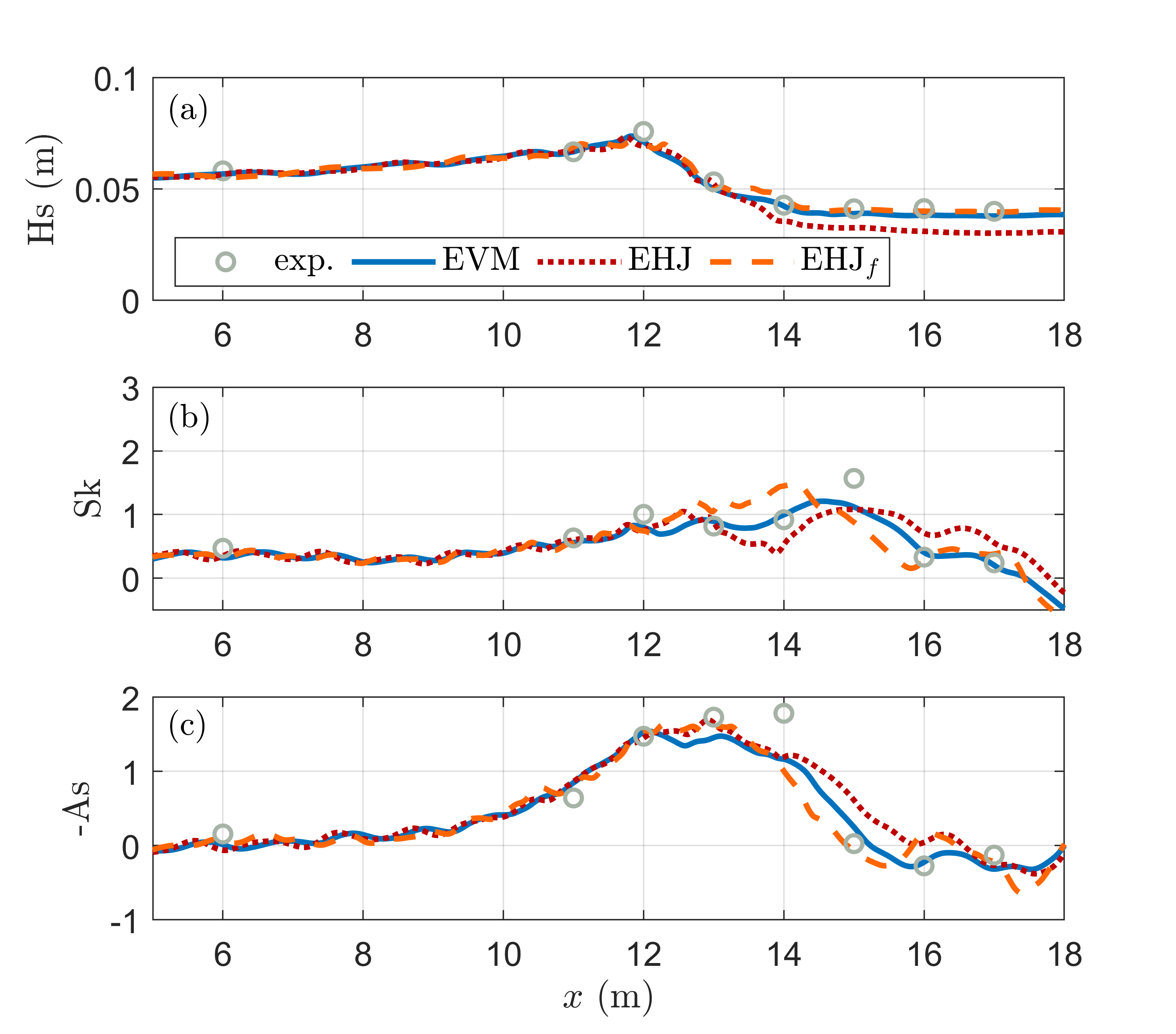
Figure 13: Spatial evolution of the (a) significant wave height Hs, (b) wave skewness Sk, and (c) wave asymmetry As, calculated over $15T$ sec, for the experimental measurements (circles), EVM (plain lines), EHJ (dotted lines), and EHJ_f (dashed lines) of the experiment of Beji and Battjes (1993).

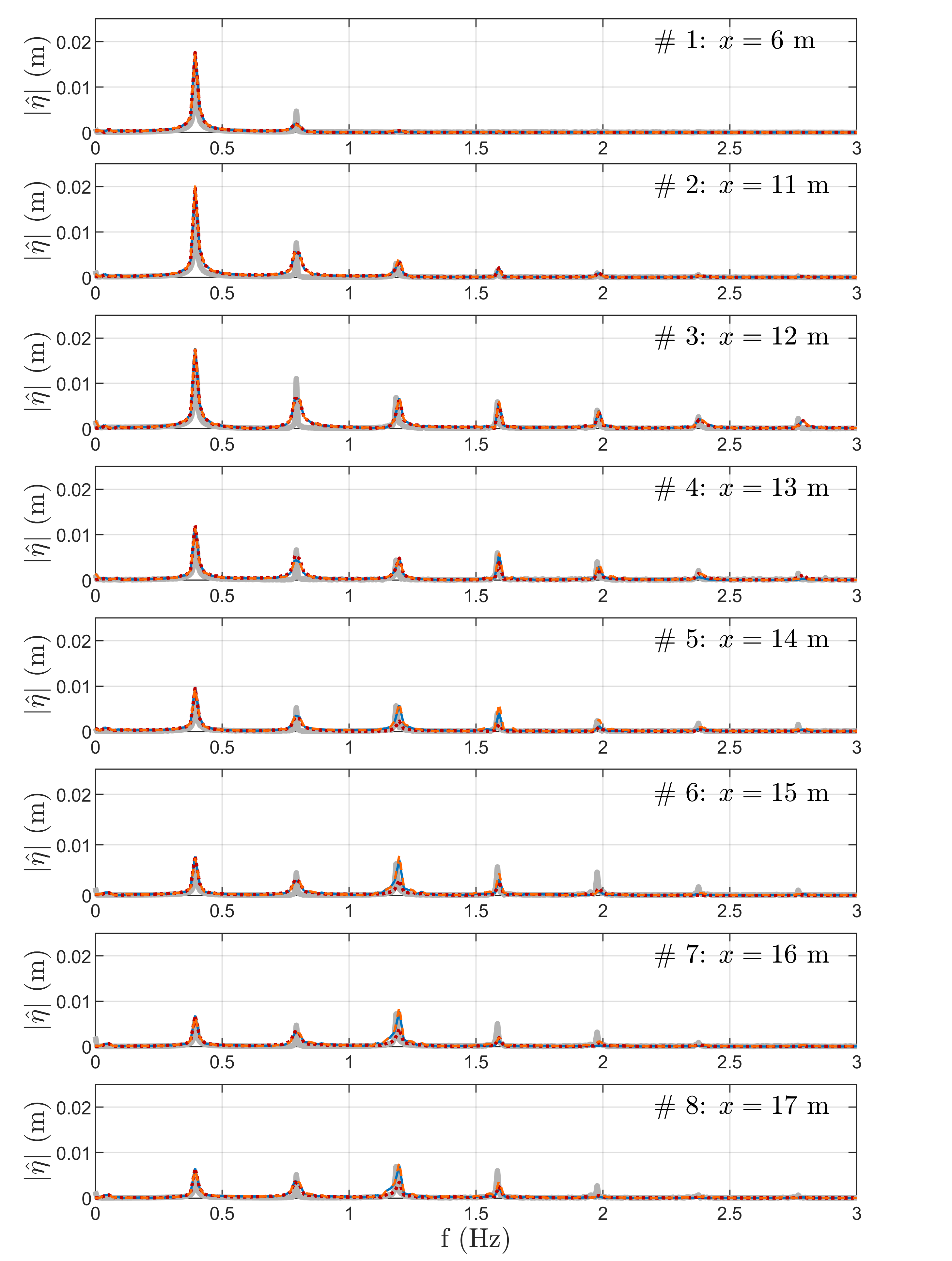
Figure 14: Comparison of the wave spectrum between the experimental data (grey line), EVM (plain lines), EHJ (dotted lines), and EHJ_f (dashed lines) for the experiment of Beji and Battjes (1993).

6 Discussion and Conclusions

In this paper, two different methods are presented for simulating the effects of wave breaking in the framework of the Hamiltonian formulation of free-surface potential flow. The first, called the EVM, is a variant of the eddy viscosity model proposed for BT models by Kennedy et al. (2000). The term introduced in the FSBC is computed by solving a differential equation derived by requiring that momentum is conserved as the waves break over a flat bottom. The second method, EHJ, is the implementation of the dissipative term proposed by Guignard and Grilli (2001) and Grilli et al. (2019). This term is constructed such that it produces negative work proportional to the work done by a hydraulic jump with wave characteristics similar to those of the breaking wave. For both methods, wave breaking events are determined by simple initiation and termination criteria as a function of the velocity of the free-surface elevation. The numerical scheme is based on the Hamiltonian Coupled-Mode Theory, which is implemented with a fourth-order spatial discretization and an explicit fourth-order Runge-Kutta time-stepping algorithm.

The proposed breaking models were applied to several test cases. The first test case verified numerically that both methods dissipate energy while conserving momentum for the propagation over a flat bottom of breaking DSWs. A laboratory dam-break problem was also successively reproduced by all three methods, with the EVM producing the best results. The overall performance of the EVM was good for all examined cases, giving particularly accurate results in the case of a plunging wave breaking over a submerged trapezoidal bar. Fair agreement with the same experiment is also obtained with the EHJ, even though this approach was originally proposed for spilling breakers on milder slopes. Here, it was also shown that restricting the breaking region of the EHJ to the front face of the breaking wave (EHJ_f variant) improves results for dispersive shock waves and plunging breakers propagating over a barred bathymetry. In the case of spilling breaking waves propagating over a mildly sloping beach, the EVM and EHJ methods reproduced well the maximum and minimum levels of the free-surface elevation. An underestimation of the increase in the mean water level after the breaking point (set-up) is obtained by both methods. This could be explained partially by the inability of the present numerical scheme to take into account a moving shoreline and by the use of a modified bathymetry and a sponge layer at the end of the wave tank. More generally, the application of energy dissipation as a pressure term into the Bernoulli FSBC may not introduce the optimal radiation stress changes in the case of spilling breakers. These issues deserve further investigation and should be the focus of future work.

To conclude, the proposed methods demonstrate promising results in water wave problems where strong nonlinearity, dispersion and wave dissipation are present. They are quite general in the sense that they can be implemented in other wave models provided that they use the free-surface potential as one of the evolving variables. Future work includes extending the present one-dimensional (1DH) approach to two horizontal dimensions (2DH). Although the performances of the two presented methods are comparable in 1DH, the extension of EVM to 2DH seems more straightforward because it does not depend on the instantaneous geometric characteristics of breaking waves. Additional future work includes the incorporation of bottom friction effects, the treatment of a moving shoreline (run-up), and the application of the models to realistic coastal applications.

Appendix A Proof of Eq. (2.12)

Differentiation of the kinetic energy term of $E$, $K=1/2\,\psi\,\mathcal{G}[\eta]\psi$, with respect to $x$ gives

$$2\partial_{x}K=\partial_{x}\psi\,\mathcal{G}[\eta]\psi+\psi\,\partial_{x}\left(\mathcal{G}[\eta]\psi\right).$$ (A.1)

The expression for the $x$-derivative of the DtN operator derived in Lannes (2013, Corollary 3.26) can be written as

$$\partial_{x}(\mathcal{G}\psi)=\mathcal{G}(\partial_{x}\psi-\mathcal{W}\psi\,\partial_{x}\eta)-\partial_{x}\big{[}(\partial_{x}\psi-\mathcal{W}\psi)\,\partial_{x}\eta\big{]},$$ (A.2)

where the simplified notation $\mathcal{G}[\eta]\psi\equiv\mathcal{G}\psi$ is introduced together with the vertical derivative of the velocity potential on the free surface,

$$\mathcal{W}\psi\equiv\mathcal{W}[\eta]\psi=\frac{\mathcal{G}\psi+\partial_{x}\eta\partial_{x}\psi}{1+(\partial_{x}\eta)^{2}}=\left[\partial_{z}\Phi\right]_{z=\eta}.$$ (A.3)

Using Eq. (A.2), the right hand side of Eq. (A.1) takes the form

$$\partial_{x}\psi\,\mathcal{G}\psi+\psi\,\mathcal{G}(\partial_{x}\psi)-\psi\,\mathcal{G}(\mathcal{W}\psi\partial_{x}\eta)-\psi\partial_{x}\big{[}\big{(}\partial_{x}\psi-\mathcal{W}\psi\,\partial_{x}\eta\big{)}\partial_{x}\eta\big{]}.$$ (A.4)

Integrating Eq. (A.1), we obtain

$$\int 2\partial_{x}Kdx=\int\left\{2\partial_{x}\psi\,\mathcal{G}\psi-\mathcal{G}\psi\,\mathcal{W}\psi\,\partial_{x}\eta+\partial_{x}\psi\big{(}\partial_{x}\psi-\mathcal{W}\psi\,\partial_{x}\eta\big{)}\partial_{x}\eta\right\}dx,$$ (A.5)

where the self-adjointness of $\mathcal{G}$ has been used to derive the second and third terms in Eq. (A.4) and the vanishing at infinity condition to derive the fourth term. By simply rearranging the above equation, it takes the form

$$\int 2\partial_{x}Kdx=\int\left\{2\partial_{x}\psi\mathcal{G}\psi+\partial_{x}\eta\Big{[}(\partial_{x}\psi)^{2}-\left(\partial_{x}\eta\partial_{x}\psi+\mathcal{G}\psi\right)\mathcal{W}\psi\Big{]}\right\}dx.$$ (A.6)

Differentiation of the potential energy term of $E$, $V=1/2g\eta^{2}$, gives

$$\int 2\partial_{x}Vdx=2g\int\eta\partial_{x}\eta dx.$$ (A.7)

Combining Eqs. (A.6) and (A.7) and taking into account Eq. (A.3), we obtain

$$\int\partial_{x}Edx=\int\left\{\partial_{x}\psi\,\mathcal{G}\psi+\partial_{x}\eta\left[g\eta+\frac{1}{2}(\partial_{x}\psi)^{2}-\frac{\big{(}\mathcal{G}\psi+\partial_{x}\psi\partial_{x}\eta\big{)}^{2}}{2\left(1+|\partial_{x}\eta|^{2}\right)}\right]\right\}dx,$$ (A.8)

which is exactly Eq. (2.12), in view of the Hamiltonian Eqs. (2.5).

Appendix B Vertical functions $Z_{n}$, $n\geq-2$

The vertical basis system $\{Z_{n}\}_{n\geq-2}$ is composed of two polynomial functions $\left\{Z_{-2},Z_{-1}\right\}$ and a set of eigenfunctions $\{Z_{n}\}_{n\geq 0}$, normalized so that $Z_{n}(\eta)=1$:

$$Z_{-2}(z;{\kern 1.0pt}\eta,{\kern 1.0pt}h) =\frac{\mu_{0}h_{0}+1}{2{\kern 1.0pt}h_{0}}{\kern 1.0pt}\frac{(z+h)}{H}^{{\kern 1.0pt}2}-\frac{\mu_{0}h_{0}+1}{2h_{0}}{\kern 1.0pt}H+1,$$ (B.1a)

$$Z_{-1}(z{\kern 1.0pt};\eta,h) =\frac{\mu_{0}h_{0}-1}{2h_{0}}{\kern 1.0pt}\frac{(z+h)}{H}^{{\kern 1.0pt}2}+{\kern 1.0pt}\frac{1}{h_{0}}{\kern 1.0pt}(z+h){\kern 1.0pt}-{\kern 1.0pt}\frac{\mu_{0}h_{0}+1}{2h_{0}}{\kern 1.0pt}H{\kern 1.0pt}+{\kern 1.0pt}1$$ (B.1b)

$$Z_{0}(z;{\kern 1.0pt}\eta,{\kern 1.0pt}h) =\frac{\cosh(k_{0}(z+h))}{\cosh(k_{0}H)},$$ (B.1c)

$$Z_{n}(z;{\kern 1.0pt}\eta,{\kern 1.0pt}h) =\frac{\cos(k_{n}(z+h))}{\cos(k_{n}H)},\quad n\geq 1,$$ (B.1d)

In Eqs. (B.1a)-(B.1d), $H=H(x,t)=\eta(x,t)+h(x)$ is the local depth of the fluid, $\mu_{0},{\kern 1.0pt}h_{0}$ are two auxiliary constants and $k_{n}=k_{n}(x,{\kern 1.0pt}t)$, $n\geq 0$ are the roots of the following transcendental equations:

$$k_{0}{\kern 1.0pt}H{\kern 1.0pt}\tanh(k_{0}{\kern 1.0pt}H) =\mu_{0}H(x,t)$$ (B.2a)

$$k_{n}{\kern 1.0pt}H{\kern 1.0pt}\tan(k_{n}{\kern 1.0pt}H) =-\mu_{0}H(x,t),\,\,\text{for}\,\,n\geq 1,$$ (B.2b)

that are efficiently solved at machine precision (Papathanasiou et al., 2018). The auxiliary constant $h_{0}$ is introduced only for dimensional purposes, and its value is taken to be a characteristic depth of the studied configuration, e.g. the depth in the incident wave region. The essential role of $\mu_{0}$ is to formulate the free-surface boundary condition of the Sturm-Liouville problem defining the eigenfunctions $\{Z_{n}\}_{n\geq 0}$ and it is chosen as $\mu_{0}=\omega_{0}^{2}/g$, where $\omega_{0}$ is the frequency of the incident wave. For more details we refer the reader to Athanassoulis and Belibassakis (1999); Belibassakis and Athanassoulis (2011); Athanassoulis and Papoutsellis (2017).

Appendix C Finite-Difference formulae

For an arbitrary function $u(x)$ discretized on a regular grid of spacing $\delta x$, first and second derivatives in space are approximated by fourth-order finite difference formulae, as:

$$(\partial_{x}u)_{i}=\\ \left\{\begin{array}[]{ll}\frac{1}{\delta x}\left(-\frac{25}{12}u_{i}+4u_{i+1}-3u_{i+2}+\frac{4}{3}u_{i+3}-\frac{1}{4}u_{i+4}\right),&i=1\\ \frac{1}{\delta x}\left(-\frac{1}{4}u_{i-1}-\frac{5}{6}u_{i}+\frac{3}{2}u_{i+1}-\frac{1}{2}u_{i+2}+\frac{1}{12}u_{i+3}\right),&i=2\\ \frac{1}{12\delta x}\left(u_{i-2}-8u_{i-1}+8u_{i+1}-u_{i+2}\right),&i=3,...,N_{X}-2\\ \frac{1}{\delta x}\left(-\frac{1}{12}u_{i-3}+\frac{1}{2}u_{i-2}-\frac{3}{2}u_{i-1}+\frac{5}{6}u_{i}+\frac{1}{4}u_{i+1}\right),&i=N_{X}-1\\ \frac{1}{\delta x}\left(\frac{1}{4}u_{i-4}-\frac{4}{3}u_{i-3}+3u_{i-2}-4u_{i-1}+\frac{25}{12}u_{i}\right),&i=N_{X}\end{array}\right.$$ (C.1)

$$(\partial^{2}_{x}u)_{i}=\\ \left\{\begin{array}[]{ll}\frac{1}{\delta^{2}}\left(\frac{15}{4}u_{i}-\frac{77}{6}u_{i+1}+\frac{107}{6}u_{i+2}-13u_{i+3}+\frac{61}{12}u_{i+4}-\frac{5}{6}u_{i+5}\right),\quad\quad i=1\\ \frac{1}{\delta^{2}}\left(\frac{5}{6}u_{i-1}-\frac{5}{4}u_{i}-\frac{1}{3}u_{i+1}+\frac{7}{6}u_{i+2}-\frac{1}{2}u_{i+3}+\frac{1}{12}u_{i+4}\right),\quad\quad\quad\quad i=2\\ \frac{1}{12\delta^{2}}\left(-u_{i-2}+16u_{i-1}-30u_{i}+16u_{i+1}-u_{i+2}\right),\quad\quad i=3,...,N_{X}-2\\ \frac{1}{\delta^{2}}\left(\frac{5}{6}u_{i+1}-\frac{5}{4}u_{i}-\frac{1}{3}u_{i-1}+\frac{7}{6}u_{i-2}-\frac{1}{2}u_{i-3}+\frac{1}{12}u_{i-4}\right),\quad\,\,\,i=N_{X}-1\\ \frac{1}{\delta^{2}}\left(\frac{15}{4}u_{i}-\frac{77}{6}u_{i-1}+\frac{107}{6}u_{i-2}-13u_{i-3}+\frac{61}{12}u_{i-4}-\frac{5}{6}u_{i-5}\right),\quad\,\,\,i=N_{X}\end{array}\right.$$ (C.2)

References

- Athanassoulis and Belibassakis (1999) Athanassoulis, G.A., Belibassakis, K.A., 1999. A consistent coupled-mode theory for the propagation of small-amplitude water waves over variable bathymetry regions. J. Fluid Mech. 389, 275–301.
- Athanassoulis et al. (2017) Athanassoulis, G.A., Belibassakis, K.A., Papoutsellis, Ch.E., 2017. An exact Hamiltonian coupled-mode system with application to extreme design waves over variable bathymetry. J. Ocean Eng. Mar. Energy 3, 373–383.
- Athanassoulis and Papoutsellis (2015) Athanassoulis, G.A., Papoutsellis, Ch.E., 2015. New form of the Hamiltonian equations for the nonlinear water-wave problem, based on a new representation of the DtN operator, and some applications., in: Proc. 34th Int. Conf. Ocean. Offshore Arct. Eng., ASME, St. John’s, Newfoundland, Canada. V007T06A029.
- Athanassoulis and Papoutsellis (2017) Athanassoulis, G.A., Papoutsellis, Ch.E., 2017. Exact semi-separation of variables in waveguides with non-planar boundaries. Proc. R. Soc. A 473, 20170017.
- Beji and Battjes (1993) Beji, S., Battjes, J.A., 1993. Experimental investigation of wave propagation over a bar. Coast. Eng. 19, 151–163.
- Belibassakis and Athanassoulis (2011) Belibassakis, K.A., Athanassoulis, G.A., 2011. A coupled-mode system with application to nonlinear water waves propagating in finite water depth and in variable bathymetry regions. Coast. Eng. 58, 337–350.
- Benjamin and Olver (1982) Benjamin, T.B., Olver, P.J., 1982. Hamiltonian structure, symmetries and conservation laws for water waves. J. Fluid Mech. 125, 137–185.
- Bingham and Zhang (2007) Bingham, H.B., Zhang, H., 2007. On the accuracy of finite difference solutions for nonlinear water waves. J. Eng. Math. 58, 211–228.
- Bonneton et al. (2011) Bonneton, P., Barthélemy, E., Chazel, F., Cienfuegos, R., Lannes, D., 2011. Recent advances in Serre-Green Naghdi modelling for wave transformation, breaking and runup processes. Eur. J. Mech. B Fluids 30, 589–597.
- Briganti et al. (2004) Briganti, R., Musumeci, R.E., Bellotti, G., Brocchini, M., Foti, E., 2004. Boussinesq modeling of breaking waves: Description of turbulence. J. Geophys. Res. 109, C07015.
- Brocchini (2013) Brocchini, M., 2013. A reasoned overview on Boussinesq-type models: the interplay between physics, mathematics and numerics. Proc. R. Soc. A 469(2160), 20130496.
- Broer (1974) Broer, L.J., 1974. On the Hamiltonian theory of surface waves. Appl. Sci. Res 30, 430–446.
- Cao et al. (1993) Cao, Y., Beck, R.F., Schultz, W.W., 1993. An absorbing beach for numerical simulations of nonlinear waves in a wave tank., in: 8th Int. Workshop Water Waves and Floating Bodies, pp. 17–20. St John’s, Newfoundland, Canada.
- do Carmo et al. (2019) do Carmo, J.S.A., Ferreira, J., Pinto, L., 2019. On the accurate simulation of nearshore and dam break problems involving dispersive breaking waves. Wave Motion 85, 125–143.
- do Carmo et al. (2018) do Carmo, J.S.A., Ferreira, J.A., Pinto, L., Romanazzi, G., 2018. An improved Serre model: Efficient simulation and comparative evaluation. Applied Mathematical Modelling 56, 404 – 423.
- do Carmo et al. (1993) do Carmo, J.S.A., Seabra-Santos, F.J., Almeida, A.B., 1993. Numerical solution of the generalized Serre equations with the McCormack finite-difference scheme. Int. J. Numer. Methods Fluids 16, 725–738.
- Chazel et al. (2011) Chazel, F., Lannes, D., Marche, F., 2011. Numerical simulation of strongly nonlinear and dispersive waves using a Green-Naghdi model. J. Sci. Comput. 48, 105–116.
- Cienfuegos et al. (2010) Cienfuegos, R., Barthélemy, E., Bonneton, P., 2010. Wave-breaking model for Boussinesq-Type equations including roller effects in the mass conservation equation. J. Waterway, Port, Coastal, Ocean Eng. 136, 10–26.
- Craig and Sulem (1993) Craig, W., Sulem, C., 1993. Numerical simulation of gravity waves. J. Comp. Phys. 108, 73–83.
- Delestre et al. (2013) Delestre, O., Lucas, C., Ksinant, P.A., Darboux, F., Laguerre, C., T.N. Tuoi Vo, James, F., Cordier, S., 2013. SWASHES: a compilation of shallow water analytic solutions for hydraulic and environmental studies . Int. J. Numer. Meth. Fluids 72, 269–300.
- Derakhti et al. (2016) Derakhti, M., Kirby, J., Shi, F., Ma, G., 2016. Wave breaking in the surf zone and deep-water in a non-hydrostatic RANS model. Part 2: Turbulence and mean circulation. Ocean Modelling 107, 139–150.
- Dommermuth and Yue (1987) Dommermuth, D.G., Yue, D.K.P., 1987. A high-order spectral method for the study of nonlinear gravity waves. J. Fluid Mech. 184, 267 – 288.
- Gagarina et al. (2014) Gagarina, E., Ambatia, V.R., van der Vegt, J.J.W., Bokhove, O., 2014. Variational space–time (dis)continuous Galerkin method for nonlinear free surface water waves . J. Comput. Phys. 275, 459–483.
- Gouin et al. (2016) Gouin, M., Ducrozet, G., Ferrant, P., 2016. Development and validation of a non-linear spectral model for water waves over variable depth. Eur. J. Mech. B Fluids 57, 115–128.
- Grilli et al. (2001) Grilli, S.T., Guyenne, P., Dias, F., 2001. A fully non-linear model for three-dimensional overturning waves over an arbitrary bottom. Int. J. Numer. Meth. Fluids 35, 829–867.
- Grilli et al. (2019) Grilli, S.T., Horillo, J., Guignard, S., 2019. Fully nonlinear potential flow simulations of wave shoaling over slopes: Spilling breaker model and integral wave properties. Water Waves doi:10.1007/s42286-019-00017-6.
- Grilli and Horrillo (1997) Grilli, S.T., Horrillo, J., 1997. Numerical generation and absorption of fully nonlinear periodic waves. J. Eng. Mech. 123, 1060–1069.
- Guignard and Grilli (2001) Guignard, S., Grilli, S.T., 2001. Modeling of wave shoaling in a 2D-NWT using a spilling breaker model, in: Proc. ISOPE 2001 Conf. Stavanger, Norway, ISOPE-I-01-253.
- Guyenne and Nicholls (2007) Guyenne, P., Nicholls, D., 2007. A high-order spectral method for nonlinear water waves over moving bottom topography. SIAM J. Sci. Comput 30, 81–101.
- Heitner and Housner (1970) Heitner, K., Housner, G., 1970. Numerical model for tsunami run-up. Coast. Eng. Div. 96, 701–719.
- Karambas and Koutitas (1992) Karambas, T.V., Koutitas, C., 1992. A breaking wave propagation model based on the Boussinesq equations. Coast. Eng. 18, 1–19.
- Karambas and Memos (2009) Karambas, T.V., Memos, C.D., 2009. Boussinesq model for weakly nonlinear fully dispersive water waves. J. Waterway, Port, Coastal, Ocean Eng. 135, 187–199.
- Kazolea et al. (2014) Kazolea, M., Delis, A.I., Synolakis, C.E., 2014. Numerical treatment of wave breaking on unstructured finite volume approximations for extended Boussinesq-type equations. J. Comp. Phys. 271, 281–305.
- Kazolea and Ricchiuto (2018) Kazolea, M., Ricchiuto, M., 2018. On wave breaking for Boussinesq-type models. Ocean Modelling 123, 16–39.
- Kennedy et al. (2000) Kennedy, A.B., Chen, Q.C., Kirby, J.T., Dalrymple, R., 2000. Boussinesq modeling of wave transformation, breaking, and runup I:1D . J. Waterway, Port, Coastal, Ocean Eng. 126, 39–47.
- Kirby (2016) Kirby, J.T., 2016. Boussinesq models and their application to coastal processes across a wide range of scales. J. Waterway, Port, Coastal, Ocean Eng. 142(6), 03116005.
- Kurnia and van Groesen (2014) Kurnia, R., van Groesen, E., 2014. High order hamiltonian water wave models with wave-breaking mechanism. Coast. Eng. 93, 55–70.
- Lannes (2013) Lannes, D., 2013. The Water Waves Problem. Mathematical Analysis and Asymptotics. volume 188 of Mathematical Surveys and Monographs. American Mathematical Society.
- Lannes and Bonneton (2009) Lannes, D., Bonneton, P., 2009. Derivation of asymptotic two-dimensional time-dependent equations for surface water wave propagation. Phys. Fluids 21, 016601.
- Madsen et al. (2006) Madsen, P.A., Fuhrman, D.R., Wang, B., 2006. A Boussinesq-type method for fully nonlinear waves interacting with a rapidly varying bathymetry. Coast. Eng. 53, 487–504.
- Madsen et al. (1997) Madsen, P.A., Sorensen, O.R., Schäffer, H.A., 1997. Surf zone dynamics simulated by a boussinesq type model. part i. model description and cross-shore motion of regular waves. Coast. Eng. 32, 255–287.
- Milder (1990) Milder, D.M., 1990. The effects of truncation on surface-wave Hamiltonians. J. Fluid Mech. 216, 249–262.
- Miles (1977) Miles, J.W., 1977. On Hamilton’s principle for surface waves. J. Fluid Mech 83, 153–158.
- Mitsotakis et al. (2017) Mitsotakis, D., Dutykh, D., Carter, J., 2017. On the nonlinear dynamics of the traveling-wave solutions of the Serre system. Wave Motion 70, 166 – 182.
- Mitsotakis et al. (2015) Mitsotakis, D., Synolakis, C.E., McGuiness, M., 2015. A modified Galerkin/Finite Element Method for the numerical solution of the Serre-Green-Nagdhi system. Int. J. Numer. Meth. 83(10), 755–778.
- Nwogu (1993) Nwogu, O.G., 1993. Alternative form of Boussinesq equations for nearshore wave propagation. J. Waterway, Port, Coastal, Ocean Eng. 119, 618–638.
- Papathanasiou et al. (2018) Papathanasiou, T., Papoutsellis, Ch.E., Athanassoulis, G.A., 2018. Semi-explicit solutions to the water-wave dispersion relation and their role in the non-linear Hamiltonian coupled-mode theory. J. Eng. Math. 114(1), 87–114.
- Papoutsellis (2016) Papoutsellis, Ch.E., 2016. Nonlinear water waves over varying bathymetry: theoretical and numerical study using variational methods. Ph.D. thesis. National Technical University of Athens. http://dspace.lib.ntua.gr/handle/123456789/44741.
- Papoutsellis and Athanassoulis (2017) Papoutsellis, Ch.E., Athanassoulis, G.A., 2017. A new efficient Hamiltonian approach to the nonlinear water-wave problem over arbitrary bathymetry http://arxiv.org/abs/1704.03276.
- Papoutsellis et al. (2018) Papoutsellis, Ch.E., Charalampopoulos, A., Athanassoulis, G.A., 2018. Implementation of a fully nonlinear Hamiltonian Coupled-Mode Theory, and application to solitary wave problems over bathymetry. Eur. J. Mech. B Fluids 72, 199–224.
- Raoult et al. (2016) Raoult, C., Benoit, M., Yates, M.L., 2016. Validation of a fully nonlinear and dispersive wave model with laboratory non-breaking experiments. Coast. Eng. 114, 194–207.
- Raoult et al. (2019) Raoult, C., Benoit, M., Yates, M.L., 2019. Development and validation of a 3D RBF-spectral model for coastal wave simulation. J. Comput. Phys. 378, 278–302.
- Roeber et al. (2010) Roeber, V., Cheung, K., Kobayashi, M., 2010. Shock-capturing Boussinesq-type model for nearshore wave processes. Coast. Eng. 57, 407–423.
- Schäffer et al. (1993) Schäffer, H., Madsen, P., Deigaard, R., 1993. A Boussinesq model for waves breaking in shallow water. Coast. Eng. 20, 185–202.
- Seiffert and Ducrozet (2017) Seiffert, B.R., Ducrozet, G., 2017. Simulation of breaking waves using the high-order spectral method with laboratory experiments: wave-breaking energy dissipation. Ocean Dynam. 68, 65–89.
- Stoker (1957) Stoker, J.J., 1957. Water Waves: The Mathematical Theory with Applications. volume 4 of Pure and Applied Mathematics. Interscience Publishers, New York.
- Svendsen (1984) Svendsen, I.A., 1984. Mass flux and undertow in a surf zone. Coast. Eng. 8, 374–365.
- Tian and Sato (2008) Tian, Y., Sato, S., 2008. A numerical model on the interaction between nearshore nonlinear waves and strong currents. Coast. Eng. J. 50, 369–395.
- Tian et al. (2010) Tian, Z., Perlin, M., Choi, W., 2010. Energy dissipation in two-dimensional unsteady plunging breakers and an eddy viscosity model. J. Fluid Mech. 655, 217–257.
- Ting and Kirby (1994) Ting, F.C.K., Kirby, J.T., 1994. Observation of undertow and turbulence in a laboratory surf zone. Coast. Eng. 24, 51–80.
- Tissier et al. (2012) Tissier, M., Bonneton, P., Marche, F., Chazel, F., Lannes, D., 2012. A new approach to handle wave breaking in fully non-linear Boussinesq models. Coast. Eng. 67, 54–66.
- Tonelli and Petti (2009) Tonelli, M., Petti, M., 2009. Hybrid finite-volume finite-difference scheme for 2DH improved Boussinesq equations. Coast. Eng. 56, 609–620.
- Veeramony and Svendsen (2000) Veeramony, J., Svendsen, I.A., 2000. The flow in surf-zone waves. Coast. Eng. 39, 93–122.
- Yates and Benoit (2015) Yates, M.L., Benoit, M., 2015. Accuracy and efficiency of two numerical methods of solving the potential flow problem for highly nonlinear and dispersive water waves. Int. J. Numer. Methods Fluids 77, 616–640.
- Zakharov (1968) Zakharov, V.E., 1968. Stability of periodic waves of finite amplitude on the surface of a deep fluid. J. Appl. Mech. Tech. Phys 9, 86–94.
- Zelt (1991) Zelt, J.A., 1991. The run-up of nonbreaking and breaking solitary waves. Coast. Eng. 15, 205–246.
- Zhao et al. (2014) Zhao, B.B., Duan, W.Y., Ertekin, R.C., 2014. Application of higher-level GN theory to some wave transformation problems. Coast. Eng. 83, 177–189.