i-RIM applied to the fastMRI challenge

Abstract

We, team AImsterdam, summarize our submission to the fastMRI challenge (Zbontar et al., 2018). Our approach builds on recent advances in invertible “learning to infer” models as presented in Putzky and Welling (2019). Both, our single-coil and our multi-coil model share the same basic architecture.

1 Introduction

To solve the accelerated MRI problem as presented in the fastMRI challenge (Zbontar et al., 2018), we train an invertible Recurrent Inference Machine (i-RIM) for each of the challenges (Putzky and Welling, 2019). The i-RIM is an invertible variant of the RIM (Putzky and Welling, 2017) which has been successfully applied to accelerated MRI before (Lønning et al., 2019). The formulation of the i-RIM allows us to stably train models which are several hundreds of layers deep. Most of our approach is already described in Putzky and Welling (2019). Here, we will focus on changes to Putzky and Welling (2019) which were done for the challenge, and on the adaptation to the multi-coil setting.

We treat the problem of accelerated MRI as an inverse problem with a forward model given by

$$\mathbf{d}^{(i)} =\mathbf{P}\mathscr{F}\mathbf{p}^{(i)}+\mathbf{n}^{(i)}$$ (1)

where $\mathbf{d}^{(i)}\in\mathbb{C}^{m}$ are sub-sampled k-space measurements at coil $i$, $\mathbf{P}$ is a sampling mask, $\mathscr{F}$ is a Fourier transform, $\mathbf{p}^{(i)}\in\mathbb{C}^{n}$ is an image recorded at coil $i$, and $\mathbf{n}^{(i)}$ is the noise at coil $i$. In our approach, we do not explicitly model spatial coil sensitivity maps as is commonly done in other approaches. We stack k-space measurement and coil images from all coils, respectively, such that the forward model takes the form

$$\mathbf{d} =\mathcal{A}\mathbf{p}+\mathbf{n}$$ (2)

with

$$\begin{aligned} \mathbf{d}=\begin{pmatrix}\mathbf{d}^{(1)}\\ \vdots\\ \mathbf{d}^{(K)}\end{pmatrix}\end{aligned}\qquad\begin{aligned} \mathbf{p}=\begin{pmatrix}\mathbf{p}^{(1)}\\ \vdots\\ \mathbf{p}^{(K)}\end{pmatrix}\end{aligned}\qquad\begin{aligned} \mathbf{n}=\begin{pmatrix}\mathbf{n}^{(1)}\\ \vdots\\ \mathbf{n}^{(K)}\end{pmatrix}\end{aligned}\qquad\begin{aligned} \mathcal{A}=\mathrm{1}_{K}\otimes\mathbf{P}\mathscr{F}\end{aligned}$$ (3)

where $\otimes$ denotes the Kronecker product, $K$ is the total number of coils in the problem, i.e. $15$ in the multi-coil setting, and $1$ in the single-coil setting.

2 Method

The i-RIM is a deep learning model which iteratively updates its machine state $(\mathbf{p}_{t},\mathbf{s}_{t})$ based on simulations of the forward model in Eq. eq:mri_measurement such that

$$\mathbf{p}_{t+1},\mathbf{s}_{t+1}=h_{\phi}(\mathcal{A},\mathbf{d},\mathbf{p}_{t},\mathbf{s}_{t})$$ (4)

where $\mathbf{p}_{t}$ is the models estimate of $\mathbf{p}$ and $\mathbf{s}_{t}$ is a latent state at iteration $t$, respectively. Many modern approaches to solving inverse problems which we refer to as “learning to infer” models can be summarized through equation Eq. eq:iterative_models. What differentiates the i-RIM from other approaches is that (1) the only model assumption is in the forward model which makes the i-RIM a mostly data-driven approach, and (2) $h_{\phi}$ is fully invertible which allows us to train the model with back-propagation without storing intermediate activations (Gomez et al., 2017). Hence, we can train arbitrarily deep networks. Empirical results in deep learning suggest that deeper models almost always perform better than their shallow counterparts (He et al., 2015). The i-RIM brings this potential to “learning to infer” models.

For the i-RIM, Eq. eq:mri_measurement specifically takes the form

$$\mathbf{p}_{t+1},\mathbf{s}_{t+1}=h_{\phi}(\nabla\mathcal{D}\left(\mathbf{d},\mathcal{A},\mathbf{p}_{t}\right),\mathbf{p}_{t},\mathbf{s}_{t})$$ (5)

where

$$\nabla\mathcal{D}\left(\mathbf{d},\mathcal{A},\mathbf{p}_{t}\right)=\mathcal{A}^{H}\left(\mathcal{A}\mathbf{p}_{t}-\mathbf{d}\right)$$

is the gradient of the data consistency term under a normal likelihood model with $\mathcal{A}^{H}$ being the adjoint operator of $\mathcal{A}$. This gradient reflects how well the current estimate is supported by the measured data under the forward model. To produce the final estimate of $\mathbf{p}$ we use a non-invertible block such that

$$\hat{\mathbf{p}}=f_{\theta}(\mathbf{p}_{T},\mathbf{s}_{T})$$ (6)

is the models final complex-valued estimate with $\hat{\mathbf{p}}\in\mathbb{C}^{n}$. The competition results are evaluated on magnitude images, hence we do $\hat{\mathbf{m}}=|\hat{\mathbf{p}}|$ to generate magnitude images for the competition. As training loss we use the structural similarity loss (Zhou Wang et al., 2004):

$$\mathcal{L}(\phi,\theta)=-\frac{1}{N}\sum_{j=1}^{N}\operatorname{SSIM}(\hat{\mathbf{m}}_{j},\mathbf{m}_{j})$$ (7)

where $N$ is the mini-batch size. As the initial machine state we set

$$\mathbf{p}_{0} =\mathcal{A}^{H}\mathbf{d}$$ (8)

$$\mathbf{s}_{0} =\begin{pmatrix}\omega\\ \mathbf{0}_{D-8}\end{pmatrix}$$ (9)

where $\mathbf{p}_{0}$ is the zero-filled corrupted image, and $\omega$ is a 1-hot vector which encodes meta-data about the experimental condition such as field strength (1.5T vs. 3T) and fat suppressed vs. non-fat suppressed data. This meta-data can potentially activate different pathways in the i-RIM under the different experimental conditions.

Models

We trained separate models for the single-coil and multi-coil challenges with 8 steps each. At each step, the models have 12 down-sampling blocks (see Putzky and Welling (2019)). In total, this amounts to 480 layer deep networks. The single-coil model has a machine state of 64 feature layers, and the multi-coil model has a machine state of 96 feature layers.

Training

Because the volumes in the data set have vastly different sizes, we cropped the central portion of each image slice to $368\times 368$ pixels. For smaller slices we applied zero padding to produce slices of the appropriate size. We simulated k-space measurements using the sampling mask function supplied by Zbontar et al. (2018) with $4\times$ and $8\times$ acceleration factors. As target images we used ESC images for the single-coil model and RSS targets for the multi-coil model, respectively (see Zbontar et al. (2018)). We used the Adam optimizer with initial learning rate $10^{-4}$ which was reduced by factor $10$ every 30 epochs.

3 Results

We evaluated our models on three data sets: the validation set as in Zbontar et al. (2018), and the test and challenge sets through the fastMRI website. A summary of these evaluations can be found in table 1. To assess image quality more closely, we show some exemplary reconstructions from each model in figure 1.

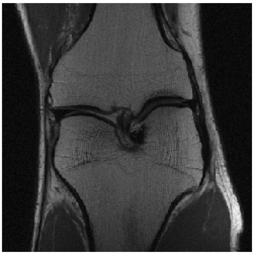
(a) Multi-Coil RSS
                                                                                                                                                 Ground Truth

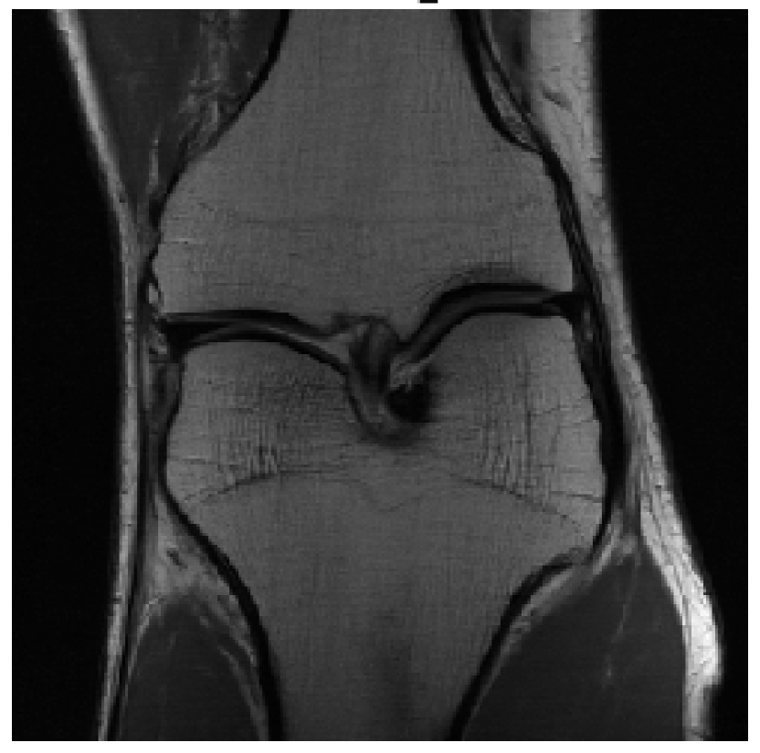
(b) Multi-Coil 4-Fold
                                                                                                                                                 Reconstruction

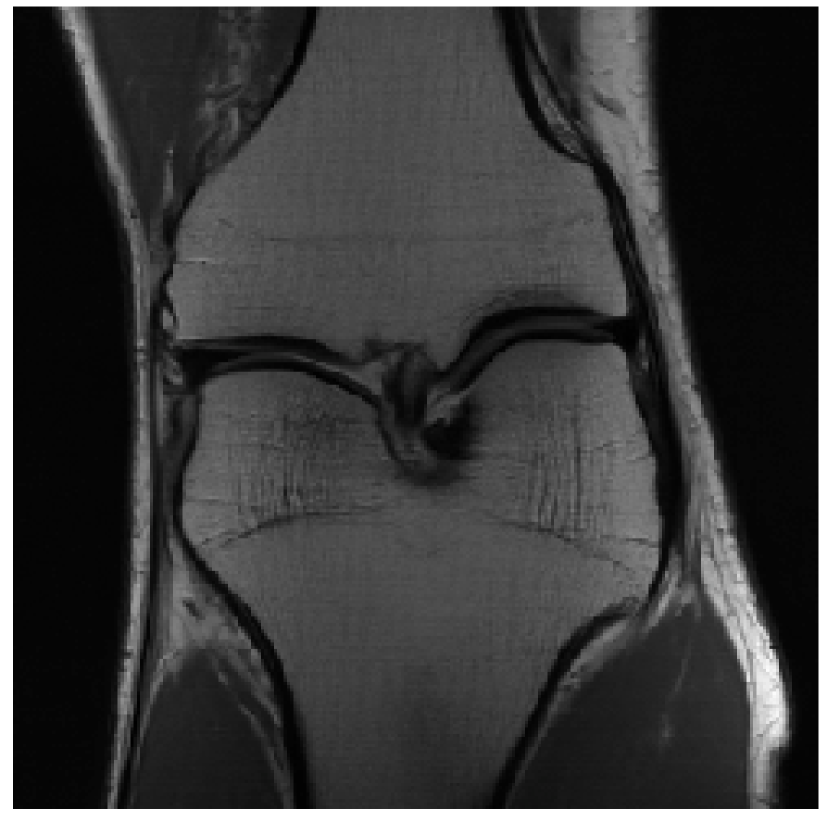
(c) Multi-Coil 8-Fold
                                                                                                                                                 Reconstruction

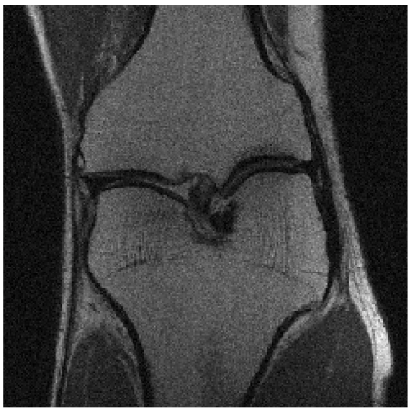
(d) Single-Coil ESC
                                                                                                                                                 Ground Truth

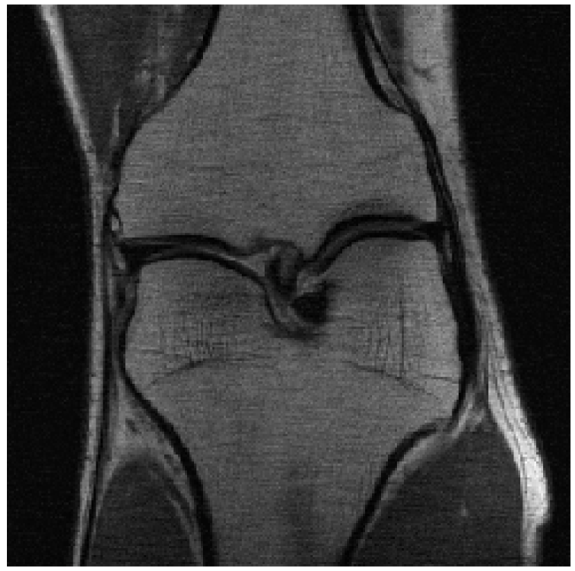
(e) Single-Coil 4-Fold
                                                                                                                                                 Reconstruction

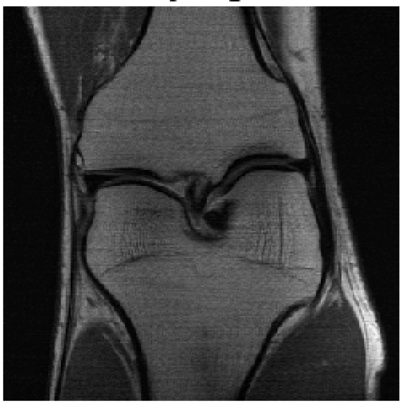
(f) Single-Coil 8-Fold
                                                                                                                                                 Reconstruction

Figure 1: Example reconstructions. The reconstructions visually improve the ground truth images, suggesting a strong prior.

Table 1: Reconstruction performance on different data sets from the fastMRI challenge Zbontar et al. (2018) under different metrics. NMSE - normalized mean-squared-error; PSNR - peak signal-to-noise ratio; SSIM - structural similarity index Zhou Wang et al. (2004). $\downarrow$ - lower is better; $\uparrow$ higher is better.

	4x Acceleration			8x Acceleration
i-RIM single-coil	NMSE $\downarrow$	PSNR $\uparrow$	SSIM $\uparrow$	NMSE $\downarrow$	PSNR $\uparrow$	SSIM $\uparrow$
Validation	$0.0342$	$32.43$	$0.751$	$0.0446$	$30.92$	$0.692$
Test	$0.0272$	$33.65$	$0.781$	$0.0421$	$30.56$	$0.687$
Challenge
i-RIM multi-coil	NMSE $\downarrow$	PSNR $\uparrow$	SSIM $\uparrow$	NMSE $\downarrow$	PSNR $\uparrow$	SSIM $\uparrow$
Validation	$0.0062$	$38.84$	$0.916$	$0.0103$	$36.19$	$0.886$
Test	$0.0052$	$39.52$	$0.928$	$0.0093$	$36.53$	$0.887$
Challenge

Acknowledgements

Patrick Putzky and Dimitrios Karkalousos were supported by Philips Research.

References

- Zbontar et al. [2018] Jure Zbontar, Florian Knoll, Anuroop Sriram, Matthew J Muckley, Mary Bruno, Aaron Defazio, Marc Parente, Krzysztof J Geras, Joe Katsnelson, Hersh Chandarana, et al. FastMRI: An open dataset and benchmarks for accelerated MRI. arXiv preprint arXiv:1811.08839, 2018.
- Putzky and Welling [2019] Patrick Putzky and Max Welling. Invert to learn to invert. In Advances in Neural Information Processing Systems 32, 2019. (accepted).
- Putzky and Welling [2017] Patrick Putzky and Max Welling. Recurrent inference machines for solving inverse problems. arXiv preprint arXiv:1706.04008, 2017.
- Lønning et al. [2019] Kai Lønning, Patrick Putzky, Jan-Jakob Sonke, Liesbeth Reneman, Matthan W.A. Caan, and Max Welling. Recurrent inference machines for reconstructing heterogeneous MRI data. Medical Image Analysis, 53:64–78, apr 2019.
- Gomez et al. [2017] Aidan N Gomez, Mengye Ren, Raquel Urtasun, and Roger B Grosse. The reversible residual network: Backpropagation without storing activations. In Advances in Neural Information Processing Systems 30. 2017.
- He et al. [2015] Kaiming He, Xiangyu Zhang, Shaoqing Ren, and Jian Sun. Deep residual learning for image recognition. arXiv preprint arXiv:1512.03385, 2015.
- Zhou Wang et al. [2004] Zhou Wang, A. C. Bovik, H. R. Sheikh, and E. P. Simoncelli. Image quality assessment: form error visibility to structural similarity. IEEE Transactions on Image Processing, 13(4):600–612, 2004.