Versatile stabilized finite element formulations for nearly and fully incompressible solid mechanics

Abstract

Computational formulations for large strain, polyconvex, nearly incompressible elasticity have been extensively studied, but research on enhancing solution schemes that offer better tradeoffs between accuracy, robustness, and computational efficiency remains to be highly relevant.

In this paper, we present two methods to overcome locking phenomena, one based on a displacement-pressure formulation using a stable finite element pairing with bubble functions, and another one using a simple pressure-projection stabilized $\mathbb{P}_{1}-\mathbb{P}_{1}$ finite element pair. A key advantage is the versatility of the proposed methods: with minor adjustments they are applicable to all kinds of finite elements and generalize easily to transient dynamics. The proposed methods are compared to and verified with standard benchmarks previously reported in the literature. Benchmark results demonstrate that both approaches provide a robust and computationally efficient way of simulating nearly and fully incompressible materials.

1 Introduction

Locking phenomena, caused by ill-conditioned global stiffness matrices in finite element analyses, are an often observed and extensively studied issue when modeling nearly incompressible, hyperelastic materials babuska1992locking (10, 18, 46, 84, 87). Typically, methods based on Lagrange multipliers are applied to enforce incompressibility. A common approach is the split of the deformation gradient into a volumetric and an isochoric part flory1961thermodynamic (38). Here, locking commonly arises when unstable standard displacement formulations are used that rely on linear shape functions to approximate the displacement field ${{\mathbf{u}}}$ and piecewise-constant finite elements combined with static condensation of the hydrostatic pressure $p$, e.g., $\mathbb{P}_{1}-\mathbb{P}_{0}$ elements. It is well known that in such cases solution algorithms may exhibit very low convergence rates and that variables of interest such as stresses can be inaccurate gultekin2018quasi (41).

From mathematical theory it is well known that approximation spaces for the primal variable ${{\mathbf{u}}}$ and $p$ have to be well chosen to fulfill the Ladyzhenskaya-Babuŝka–Brezzi (LBB) or inf-sup condition babuska1973finite (9, 19, 26) to guarantee stability. A classical stable approximation pair is the Taylor–Hood element taylor1973numerical (78), however, this requires quadratic ansatz functions for the displacement part. For certain types of problems higher order interpolations can improve efficiency as higher accuracy is already reached with coarser discretizations chamberland2010comparison (25, 57). In many applications though, where geometries are fitted to, e.g., capture fine structural features, this is not beneficial due to a possible increase in degrees of freedom and consequently a higher computational burden. Also for coupled problems such as electromechanical or fluid-structure-interaction models high-resolution grids for mechanical problems are sometimes required when interpolations between grids are not desired augustin2016anatomically (5, 51). As a remedy for these kind of applications quasi Taylor–Hood elements with an order of $\tfrac{3}{2}$ have been considered, see quaglino2017quasi (62), as well as equal order linear pairs of ansatz functions which has been a field of intensive research in the last decades, see auricchio2017mixed (7, 48) and references therein. Unfortunately, equal order pairings do not fulfill the LBB conditions and hence a stabilization of the element is of crucial importance. There is a significant body of literature devoted to stabilized finite elements for the Stokes and Navier–Stokes equations. Many of those methods were extended to incompressible elasticity, amongst other approaches by Hughes, Franca, Balestra, and collaborators franca1988new (39, 47). Masud and co-authors followed an idea by means of variational multiscale (VMS) methods masud2013framework (58, 59, 60, 85), a technique that was recently extended to dynamic problems (D-VMS) scovazzi2016simple (71, 66). Further stabilizations of equal order finite elements include orthogonal sub-scale methods chiumenti2015mixed (27, 30, 54, 24) and methods based on pressure projections dohrmann2004stabilized (33, 86). Different classes of methods to avoid locking for nearly incompressible elasticity were conceived by introducing nonconforming finite elements such as the Crouzeix–Raviart element dipietro2014extension (32, 37) and Discontinuous Galerkin methods kabaria2015hybridizable (49, 80). Enhanced strain formulations Reese1998 (63, 79) have been considered as well as formulations based on multi-field variational principles bonet2015computational (17, 68, 69).

In this study we introduce a novel variant of the MINI element for accurately solving nearly and fully incompressible elasticity problems. The MINI element was originally established for computational fluid dynamics problems arnold1984stable (3) and pure tetrahedral meshes and previously used in the large strain regime, e.g. in chamberland2010comparison (25, 55). We extend the MINI element definition for hexahedral meshes by introducing two bubble functions in the element and provide a novel proof of stability and well-posedness in the case of linear elasticity. The support of the bubble functions is restricted to the element and can thus be eliminated from the system using static condensation. This also allows for a straightforward inclusion in combination with existing finite element codes since all required implementations are purely on the element level. Additionally, we introduce a pressure-projection stabilization method originally published for the Stokes equations bochev2006 (14, 33) and previously used for large strain nearly incompressible elasticity in the field of particle finite element methods and plasticity rodriguez2016 (65, 22). Due to its simplicity, this type of stabilization is especially attractive from an implementation point of view.

Robustness and performance of both the MINI element and the pressure-projection approach are verified and compared to standard benchmarks reported previously in literature. A key advantage of the proposed methods is their high versatility: first, they are readily applicable to nearly and fully incompressible solid mechanics; second, with little adjustments the stabilization techniques can be applied to all kinds of finite elements, in this study we investigate the performance for hexahedral and tetrahedral meshes; and third, the methods generalize easily to transient dynamics.

Real world applications often require highly-resolved meshes and thus efficient and massively parallel solution algorithms for the linearized system of equations become an important factor to deal with the resulting computational load. We solve the arising saddle-point systems by using a GMRES method with a block preconditioner based on an algebraic multigrid (AMG) approach. Extending our previous implementations augustin2016anatomically (5) we performed the numerical simulations with the software Cardiac Arrhythmia Research Package (CARP) vigmond2008solvers (82) which relies on the MPI based library PETSc petsc-user-ref (12) and the incorporated solver suite hypre/BoomerAMG henson2002boomeramg (43). The combination of these advanced solving algorithms with the proposed stable elements which only rely on linear shape functions proves to be very efficient and renders feasible simulations on grids with high structural detail.

The paper is outlined as follows: Section 2 summarizes in brief the background on the methods. In Section 3, we introduce the finite element discretization and discuss stability. Subsequently, Section 4 documents benchmark problems where our proposed elements are applied and compared to results published in the literature. Finally, Section 5 concludes the paper with a discussion of the results and a brief summary.

2 Continuum mechanics

2.1 Nearly incompressible nonlinear elasticity

Let $\Omega_{0}\subset\mathbb{R}^{3}$ denote the reference configuration and let $\Omega_{t}\subset\mathbb{R}^{3}$ denote the current configuration of the domain of interest. Assume that the boundary of $\Omega_{0}$ is decomposed into $\partial\Omega_{0}=\Gamma_{\mathrm{D},0}\cup\Gamma_{\mathrm{N},0}$ with $|\Gamma_{D,0}|>0$. Here, $\Gamma_{\mathrm{D},0}$ describes the Dirichlet part of the boundary and $\Gamma_{\mathrm{N},0}$ describes the Neumann part of the boundary, respectively. Further, let ${{\mathbf{n}}}_{0}$ be the unit outward normal on $\partial\Omega_{0}$. The nonlinear mapping $\bm{\phi}\colon\bm{\mathbf{X}}\in\Omega_{0}\rightarrow{{\mathbf{x}}}\in\Omega_{t}$, defined by $\bm{\phi}:=\bm{\mathbf{X}}+{{\mathbf{u}}}(\bm{\mathbf{X}},t)$, with displacement ${{\mathbf{u}}}$, maps points in the reference configuration to points in the current configuration. Following standard notation we introduce the deformation gradient $\bm{F}$ and the Jacobian $J$ as

$$\bm{F}:=\operatorname{Grad}\bm{\phi}=\bm{I}+\operatorname{Grad}{{\mathbf{u}}},\quad J:=\det(\bm{F}),$$

and the left Cauchy-Green tensor as $\bm{C}:=\bm{F}^{\top}\bm{F}$. Here, $\operatorname{Grad}(\bullet)$ denotes the gradient with respect to the reference coordinates $\underline{X}\in\Omega_{0}$. The displacement field ${{\mathbf{u}}}$ is sought as infimizer of the functional

$$\Pi^{\mathrm{tot}}({{\mathbf{u}}}) :=\Pi({{\mathbf{u}}})+\Pi^{\mathrm{ext}}({{\mathbf{u}}}),$$

$$\Pi({{\mathbf{u}}}) :=\int\limits_{\Omega_{0}}\Psi(\bm{F}({{\mathbf{u}}}))\,\mathrm{d}\bm{\mathbf{X}},$$

$$\Pi^{\mathrm{ext}}({{\mathbf{u}}}) :=-\rho_{0}\int\limits_{\Omega_{0}}{{\mathbf{f}}}({{\mathbf{x}}})\cdot{{\mathbf{u}}}\,\mathrm{d}\bm{\mathbf{X}}-\int\limits_{\Gamma_{\mathrm{N,0}}}{{\mathbf{h}}}({{\mathbf{x}}})\cdot{{\mathbf{u}}}\,\mathrm{d}s_{\bm{\mathbf{X}}},$$ (1)

over all admissible fields ${{\mathbf{u}}}$ with ${{\mathbf{u}}}={{\mathbf{g}}}_{\mathrm{D}}$ on $\Gamma_{\mathrm{D,0}}$, where, $\Psi$ denotes the strain energy function; $\rho_{0}$ denotes the material density in reference configuration; ${{\mathbf{f}}}$ denotes a volumetric body force; ${{\mathbf{g}}}_{\mathrm{D}}$ denotes a given boundary displacement; and ${{\mathbf{h}}}$ denotes a given surface traction. For ease of presentation it is assumed that $\rho_{0}$ is constant and ${{\mathbf{f}}}$, ${{\mathbf{g}}}_{\mathrm{D}}$, and ${{\mathbf{h}}}$ do not depend on ${{\mathbf{u}}}$. Existence of infimizers is, under suitable assumptions, guaranteed by the pioneering works of Ball, see Ball1976 (13).

In this study we consider nearly incompressible materials, meaning that $J\approx 1$. A possibility to model this behavior was originally proposed by flory1961thermodynamic (38) using a split of the deformation gradient $\bm{F}$ such that

$$\bm{F}=\bm{F}_{\mathrm{vol}}\overline{\bm{F}}.$$ (2)

Here, $\bm{F}_{\mathrm{vol}}$ describes the volumetric change while $\overline{\bm{F}}$ describes the isochoric change. By setting $\bm{F}_{\mathrm{vol}}:=J^{\frac{1}{3}}\bm{I}$ and $\overline{\bm{F}}:=J^{-\frac{1}{3}}\bm{F}$ we get $\det(\overline{\bm{F}})=1$ and $\det(\bm{F}_{\mathrm{vol}})=J$. Analogously, by setting $\bm{C}_{\mathrm{vol}}:=J^{\frac{2}{3}}\bm{I}$ and $\overline{\bm{C}}:=J^{-\frac{2}{3}}\bm{C}$, we have $\bm{C}=\bm{C}_{\mathrm{vol}}\overline{\bm{C}}$. Assuming a hyperelastic material, the Flory split also postulates an additive decomposition of the strain energy function

$$\Psi=\Psi(\bm{C})=\overline{\Psi}(\overline{\bm{C}})+\kappa U(J),$$ (3)

where $\kappa$ is the bulk modulus. The function $U(J)$ acts as a penalization of incompressibility and we require that it is strictly convex and twice continuously differentiable. Additionally, a constitutive model for $U(J)$ should fulfill that (i) it vanishes in the reference configuration and that (ii) an infinite amount of energy is required to shrink the body to a point or to expand it indefinitely, i.e.,

$$\mbox{(i)}\ U(1)=0,\ \mbox{(ii)}\lim_{J\to 0+}U(J)=\infty,\ \lim_{J\to\infty}U(J)=\infty.$$

For the remainder of this work we will focus on functions $U(J)$ that can be written as

$$U(J):=\frac{1}{2}{(\Theta(J))}^{2}.$$

In the literature many different choices for the function $\Theta(J)$ are proposed, see, e.g., doll2000on (34, 42, 66) for examples and related discussion.

As we also want to study the case of full incompressibility, meaning $\kappa\to\infty$, we need a reformulation of the system. In this work we will use a perturbed Lagrange-multiplier functional, see sussman1987finite (77, 4, 21) for details, and we introduce

$$\Pi^{\mathrm{PL}}({{\mathbf{u}}},q):=\int\limits_{\Omega_{0}}\overline{\Psi}(\overline{\bm{C}}({{\mathbf{u}}}))+q\Theta(J({{\mathbf{u}}}))-\frac{1}{2\kappa}q^{2}\,\mathrm{d}\bm{\mathbf{X}}.$$

We will now seek infimizers $({{\mathbf{u}}},p)\in V_{{{\mathbf{g}}}_{\mathrm{D}}}\times Q$ of the modified functional

$$\Pi^{\mathrm{tot}}({{\mathbf{u}}},q):=\Pi^{\mathrm{PL}}({{\mathbf{u}}},q)+\Pi^{\mathrm{ext}}({{\mathbf{u}}}).$$ (4)

To guarantee that the discretization of (4) is well defined, we assume that

$$V_{{{\mathbf{g}}}_{\mathrm{D}}}=\{{{\mathbf{v}}}\in{[H^{1}(\Omega_{0})]}^{3}:\left.{{\mathbf{v}}}\right|_{\Gamma_{\mathrm{D},0}}={{\mathbf{g}}}_{\mathrm{D}}\},$$

with $H^{1}(\Omega_{0})$ being the standard Sobolev space consisting of all square integrable functions with square integrable gradient, and $Q=L^{2}(\Omega_{0})$. Existence of infimizers in $V_{{{\mathbf{g}}}_{\mathrm{D}}}$ cannot be guaranteed in general. However, assuming suitable growth conditions on the strain energy function $\Psi$, and assuming that the initial data keeps the material in the hyperelastic range, one can conclude that the space $V$ for the infimizer ${{\mathbf{u}}}$ contains $V_{{{\mathbf{g}}}_{\mathrm{D}}}$ as a subset, see Ball1976 (13) for details.

To solve for the infimizers of (4) we require to compute the variations of (4) with respect to $\Delta{{\mathbf{u}}}$ and $\Delta p$

$$D_{\Delta{{\mathbf{v}}}}\Pi^{\mathrm{PL}}({{\mathbf{u}}},p) =\int\limits_{\Omega_{0}}\left(\bm{S}_{\mathrm{isc}}+p\bm{S}_{\mathrm{vol}}\right):\bm{\Sigma}({{\mathbf{u}}},\Delta{{\mathbf{v}}})\,\mathrm{d}\bm{\mathbf{X}}$$

$$-\rho_{0}\int\limits_{\Omega_{0}}{{\mathbf{f}}}\cdot\Delta{{\mathbf{v}}}\,\mathrm{d}\bm{\mathbf{X}}-\int\limits_{\Gamma_{\mathrm{N},0}}{{\mathbf{h}}}\cdot\Delta{{\mathbf{v}}}\,\mathrm{d}s_{\bm{\mathbf{X}}},$$ (5)

$$D_{\Delta q}\Pi^{\mathrm{PL}}({{\mathbf{u}}},p) =\int\limits_{\Omega_{0}}\left(\Theta(J)-\frac{1}{\kappa}p\right)\Delta q\,\mathrm{d}\bm{\mathbf{X}},$$ (6)

with abbreviations as, e.g., in holzapfel2000nonlinear (45)

$$\bm{S}_{\mathrm{isc}} :=J^{-\frac{2}{3}}\mathrm{Dev}(\overline{\bm{S}}),\quad\text{where~{}}\overline{\bm{S}}:=\frac{\partial\overline{\Psi}(\overline{\bm{C}})}{\partial\overline{\bm{C}}}$$ (7)

$$\bm{S}_{\mathrm{vol}} :=\pi(J)\bm{C}^{-1},\quad\text{with~{}}\pi(J):=J\Theta^{\prime}(J),$$ (8)

$$\bm{\Sigma}({{\mathbf{u}}},{{\mathbf{v}}}) :=\mathrm{sym}(\bm{F}^{\top}({{\mathbf{u}}})\operatorname{Grad}{{\mathbf{v}}}).$$ (9)

Next, with notations

$$a_{\mathrm{isc}}({{\mathbf{u}}};\Delta{{\mathbf{v}}}) :=\int\limits_{\Omega_{0}}\bm{S}_{\mathrm{isc}}({{\mathbf{u}}}):\bm{\Sigma}({{\mathbf{u}}},\Delta{{\mathbf{v}}})\,\mathrm{d}\bm{\mathbf{X}},$$ (10)

$$a_{\mathrm{vol}}({{\mathbf{u}}},p;\Delta{{\mathbf{v}}}) :=\int\limits_{\Omega_{0}}p\bm{S}_{\mathrm{vol}}({{\mathbf{u}}}):\bm{\Sigma}({{\mathbf{u}}},\Delta{{\mathbf{v}}})\,\mathrm{d}\bm{\mathbf{X}},$$ (11)

$$b_{\mathrm{vol}}({{\mathbf{u}}};\Delta q) :=\int\limits_{\Omega_{0}}\Theta(J({{\mathbf{u}}}))\Delta q\,\mathrm{d}\bm{\mathbf{X}},$$ (12)

$$c(p,\Delta q) :=\frac{1}{\kappa}\int\limits_{\Omega_{0}}p\Delta q\,\mathrm{d}\bm{\mathbf{X}},$$ (13)

$$l_{\mathrm{body}}(\Delta{{\mathbf{v}}}) :=\rho_{0}\int\limits_{\Omega_{0}}{{\mathbf{f}}}\cdot\Delta{{\mathbf{v}}}\,\mathrm{d}\bm{\mathbf{X}},$$ (14)

$$l_{\mathrm{surface}}(\Delta{{\mathbf{v}}}) :=\int\limits_{\Gamma_{\mathrm{N},0}}{{\mathbf{h}}}\cdot\Delta{{\mathbf{v}}}\,\mathrm{d}s_{\bm{\mathbf{X}}},$$ (15)

$$R_{\mathrm{upper}}({{\mathbf{u}}},p;\Delta{{\mathbf{v}}}) :=a_{\mathrm{isc}}({{\mathbf{u}}};\Delta{{\mathbf{v}}})+a_{\mathrm{vol}}({{\mathbf{u}}},p;\Delta{{\mathbf{v}}})$$

$$-l_{\mathrm{body}}(\Delta{{\mathbf{v}}})-l_{\mathrm{surface}}(\Delta{{\mathbf{v}}}),$$ (16)

$$R_{\mathrm{lower}}({{\mathbf{u}}},p;\Delta q) :=b_{\mathrm{vol}}({{\mathbf{u}}};\Delta q)-c(p,\Delta q),$$ (17)

we formulate the mixed boundary value problem of nearly incompressible nonlinear elasticity via a nonlinear system of equations. This yields a nonlinear saddle-point problem, find $({{\mathbf{u}}},p)\in V_{{{\mathbf{g}}}_{D}}\times Q$ such that

$$R_{\mathrm{upper}}({{\mathbf{u}}},p;\Delta{{\mathbf{v}}}) =0,$$ (18)

$$R_{\mathrm{lower}}({{\mathbf{u}}},p;\Delta q) =0,$$ (19)

for all $(\Delta{{\mathbf{v}}},\Delta q)\in V_{{{\mathbf{0}}}}\times Q$.

2.2 Consistent linearization

To solve the nonlinear variational equations (18)–(19), with a finite element approach we first apply a Newton–Raphson scheme, for details we refer to deuflhard2011newton (31). Given a nonlinear and continuously differentiable operator $F\colon X\to Y$ a solution to $F(x)=0$ can be approximated by

$$x^{k+1} =x^{k}+\Delta x,$$

$$\left.\frac{\partial F}{\partial x}\right|_{x=x^{k}}\Delta x =-F(x^{k}),$$

which is looped until convergence. In our case, we have $X=V_{{{\mathbf{g}}}_{D}}\times Q$, $Y=\mathbb{R}^{2}$, $\Delta x={(\Delta{{\mathbf{u}}},\Delta p)}^{\top}$, $x^{k}={({{\mathbf{u}}}^{k},p^{k})}^{\top}$, and $F={(R_{\mathrm{upper}},R_{\mathrm{lower}})}^{\top}$. We obtain the following linear saddle-point problem for each $({{\mathbf{u}}}^{k},p^{k})\in V_{{{\mathbf{g}}}_{D}}\times Q$, find $(\Delta{{\mathbf{u}}},\Delta p)\in V_{{{\mathbf{0}}}}\times Q$ such that

$$a_{k}(\Delta{{\mathbf{u}}},\Delta{{\mathbf{v}}})+b_{k}(\Delta p,\Delta{{\mathbf{v}}}) =-R_{\mathrm{upper}}({{\mathbf{u}}}^{k},p^{k};\Delta{{\mathbf{v}}}),$$ (20)

$$b_{k}(\Delta q,\Delta{{\mathbf{u}}})-c(\Delta p,\Delta q) =-R_{\mathrm{lower}}({{\mathbf{u}}}^{k},p^{k};\Delta q),$$ (21)

where

$$a_{k}(\Delta{{\mathbf{u}}},\Delta{{\mathbf{v}}}) :=\int\limits_{\Omega_{0}}\operatorname{Grad}\Delta{{\mathbf{v}}}\bm{S}_{\mathrm{tot},k}:\operatorname{Grad}\Delta{{\mathbf{u}}}\,\mathrm{d}\bm{\mathbf{X}}$$

$$+\int\limits_{\Omega_{0}}\bm{\Sigma}({{\mathbf{u}}}_{k},\Delta{{\mathbf{v}}}):\mathbb{C}_{\mathrm{tot},k}:\bm{\Sigma}({{\mathbf{u}}}_{k},\Delta{{\mathbf{u}}})\,\mathrm{d}\bm{\mathbf{X}},$$

$$b_{k}(\Delta p,\Delta{{\mathbf{v}}}) :=\int\limits_{\Omega_{0}}\Delta p\pi(J_{k})\bm{F}^{-\top}_{k}:\operatorname{Grad}\Delta{{\mathbf{v}}}\,\mathrm{d}\bm{\mathbf{X}},$$

with abbreviations

$$\bm{F}_{k} :=\bm{F}({{\mathbf{u}}}_{k}),$$

$$J_{k} :=\det(\bm{F}_{k}),$$

$$\bm{S}_{\mathrm{tot},k} :=\left.\bm{S}_{\mathrm{isc}}\right|_{{{\mathbf{u}}}={{\mathbf{u}}}_{k}}+p_{k}\left.\bm{S}_{\mathrm{vol}}\right|_{{{\mathbf{u}}}={{\mathbf{u}}}_{k}},$$ (22)

$$\mathbb{C}_{\mathrm{tot},k} :=\left.\mathbb{C}_{\mathrm{isc}}\right|_{{{\mathbf{u}}}={{\mathbf{u}}}_{k}}+p_{k}\left.\mathbb{C}_{\mathrm{vol}}\right|_{{{\mathbf{u}}}={{\mathbf{u}}}_{k}},$$ (23)

$$\mathbb{C}_{\mathrm{vol}} :=k(J)\bm{C}^{-1}\otimes\bm{C}^{-1}-2\pi(J)\bm{C}^{-1}\odot\bm{C}^{-1},$$

$$k(J) :=J^{2}\Theta^{\prime\prime}(J)+J\Theta^{\prime}(J),$$

where $\mathbb{C}_{\mathrm{isc}}$ is given in (57). The derivation of the consistent linearization is lengthy but standard, we refer to (holzapfel2000nonlinear, 45, Chapter 8) for details. The definition of the higher order tensor and other abbreviations are given in the Appendix.

2.3 Review on solvability of the linearized problem

Since (20)–(21) is a linear saddle-point problem for each given $({{\mathbf{u}}}^{k},p^{k})$ we can rely on the well-established Babuška–Brezzi theory, see boffi2013mixed (15, 36, 67, 70). The crucial properties to guarantee that the problem (20)–(21) is well-posed are continuity of all involved bilinear forms and the following three conditions:

• The inf-sup condition: there exists $c_{1}>0$ such that

  $$\underset{q\in Q}{\inf}\ \underset{{{\mathbf{v}}}\in V_{{{\mathbf{0}}}}}{\sup}\frac{b_{k}(q,{{\mathbf{v}}})}{{\left\lVert{{{\mathbf{v}}}}\right\rVert}_{V_{{{\mathbf{0}}}}}{\left\lVert{q}\right\rVert}_{Q}}\geq c_{1}.$$ (24)

• The coercivity on the kernel condition: there exists $c_{2}>0$ such that

  $$a_{k}({{\mathbf{v}}},{{\mathbf{v}}})\geq c_{2}{\left\lVert{{{\mathbf{v}}}}\right\rVert}_{V_{{{\mathbf{0}}}}}^{2} \text{for all }{{\mathbf{v}}}\in\ker B,$$ (25)

  where

  $$\ker B:=\left\{{{\mathbf{v}}}\in V_{{{\mathbf{0}}}}:b_{k}(q,{{\mathbf{v}}})=0~{}\text{for all }q\in Q\right\}.$$

• Positivity of $c$: it holds

  $$c(q,q)\geq 0 \text{for all }q\in Q.$$ (26)

Upon observing that $\bm{F}^{-\top}:\operatorname{Grad}{{\mathbf{v}}}=\operatorname{div}{{{\mathbf{v}}}}$, see holzapfel2000nonlinear (45), we rewrite the bilinear form $b_{k}(q,{{\mathbf{v}}})$ as

$$b_{k}(q,{{\mathbf{v}}}) =\int\limits_{\Omega_{0}}q\pi(J_{k})\bm{F}^{-\top}_{k}:\operatorname{Grad}{{\mathbf{v}}}\,\mathrm{d}\bm{\mathbf{X}}$$

$$=\int\limits_{\Omega_{0}}q\pi(J_{k})\operatorname{div}{{{\mathbf{v}}}}\,\mathrm{d}\bm{\mathbf{X}}$$

$$=\int\limits_{\Omega_{t}}q\Theta^{\prime}(J_{k})\operatorname{div}{{{\mathbf{v}}}}\,\mathrm{d}{{\mathbf{x}}}.$$ (27)

Assuming that $\Theta^{\prime}(J)\geq 1$, we can conclude the inf-sup condition from standard arguments, see (weise2014, 83, Section 5.2). The positivity of the bilinear form $c$ is always fulfilled. However, it is not possible to show the coercivity condition (25) for a general hyperelastic material or load configuration. Nevertheless, for some special cases it is possible to establish a result. We refer to weise2014 (83, 8, 6) for a more detailed discussion. Henceforth, we will assume that our given input data is such that we stay in the range of stability of the problem. Examples for cases in which bilinear form $a_{k}$ lacks coercivity can be found in (weise2014, 83, Chapter 9) and (auricchio2010importance, 6, Section 4).

3 Finite element approximation and stabilization

Let $\mathcal{T}_{h}$ be a finite element partitioning of $\overline{\Omega}$ into subdomains, in our case either tetrahedral or convex hexahedral elements. The partitioning is assumed to fulfill standard regularity conditions, see ciarlet2002finite (29). Let $\hat{K}$ be the reference element, and for $K\in\mathcal{T}_{h}$ denote by $F_{\mathrm{K}}$ the affine, or trilinear mapping from $\hat{K}$ onto $K$. We assume that $F_{\mathrm{K}}$ is a bijection. For a tetrahedral element $K$ this can be assured whenever $K$ is non-degenerate, however, for hexahedral elements this may not necessary be the case, see knabner2003 (53) for details. Further, let $\hat{\mathbb{V}}$ and $\hat{\mathbb{Y}}$ denote two polynomial spaces defined over $\hat{K}$. We denote by

$$V_{h,0} :=\left\{{{\mathbf{v}}}\in H^{1}_{0}(\Omega_{0}):{{\mathbf{v}}}=\hat{{{\mathbf{v}}}}\circ F_{\mathrm{K}}^{-1},\hat{{{\mathbf{v}}}}\in{[\hat{\mathbb{V}}]}^{3},\forall K\in\mathcal{T}_{h}\right\},$$ (28)

$$Q_{h} :=\left\{q\in L^{2}(\Omega_{0}):p=\hat{p}\circ F_{\mathrm{K}}^{-1},\hat{p}\in\hat{\mathbb{Y}},\forall K\in\mathcal{T}_{h}\right\},$$ (29)

$$V_{h,{{\mathbf{g}}}_{\mathrm{D}}} :=H^{1}_{{{\mathbf{g}}}_{\mathrm{D}}}(\Omega_{0})\cap V_{h,0},$$ (30)

the spaces needed for further analysis in the following sections.

3.1 Nearly incompressible linear elasticity

boffi2017remark (16, 72, 73)

As a model problem we study the well-known equations for nearly incompressible linear elasticity. In this case it is assumed that $\Omega:=\Omega_{0}\approx\Omega_{t}$. Then, the linear elasticity problem reads: find $({{\mathbf{u}}},p)\in V_{{{\mathbf{g}}}_{D}}\times Q$ such that

$$2\mu\int\limits_{\Omega}\bm{\varepsilon}({{\mathbf{u}}}):\bm{\varepsilon}({{\mathbf{v}}})\,\mathrm{d}{{\mathbf{x}}}+\int\limits_{\Omega}p\operatorname{div}{{\mathbf{v}}}\,\mathrm{d}\bm{\mathbf{x}} =\int\limits_{\Omega}{{\mathbf{f}}}\cdot{{\mathbf{v}}}\,\mathrm{d}\bm{\mathbf{x}}$$ (31)

$$\int\limits_{\Omega}\operatorname{div}{{\mathbf{u}}}q\,\mathrm{d}\bm{\mathbf{x}}-\frac{1}{\lambda}\int\limits_{\Omega}pq\,\mathrm{d}\bm{\mathbf{x}} =0$$ (32)

for all $({{\mathbf{v}}},q)\in V_{{{\mathbf{0}}}}\times Q$. Here, $\mu>0$ and $\lambda$ denote the Lamé parameters, and $\bm{\varepsilon}({{\mathbf{v}}}):=\mathrm{sym}(\operatorname{grad}{{\mathbf{v}}})$.

The regularity of (31)–(32) is a classical result steinbach2008numerical (75) and follows with the same arguments as for the Stokes equations. The discretized analogue of (31)–(32) is: find $({{\mathbf{u}}}_{h},p_{h})\in V_{h,{{\mathbf{g}}}_{D}}\times Q_{h}$ such that

$$2\mu\int\limits_{\Omega}\bm{\varepsilon}({{\mathbf{u}}}_{h}):\bm{\varepsilon}({{\mathbf{v}}}_{h})\,\mathrm{d}{{\mathbf{x}}}+\int\limits_{\Omega}p_{h}\operatorname{div}{{\mathbf{v}}}_{h}\,\mathrm{d}\bm{\mathbf{x}} =\int_{\Omega}{{\mathbf{f}}}\cdot{{\mathbf{v}}}_{h}\,\mathrm{d}\bm{\mathbf{x}}$$ (33)

$$\int\limits_{\Omega}\operatorname{div}{{\mathbf{u}}}_{h}q_{h}\,\mathrm{d}\bm{\mathbf{x}}-\frac{1}{\lambda}\int\limits_{\Omega}p_{h}q_{h}\,\mathrm{d}\bm{\mathbf{x}} =0$$ (34)

for all $({{\mathbf{v}}}_{h},q_{h})\in V_{h,{{\mathbf{0}}}}\times Q_{h}$. Coercivity on the kernel condition (25) is a standard result for the case of nearly incompressible linear elasticity posed in the form (31)-(32) and (33)-(34). In the nonlinear case this is not true in general and will be adressed in Section 3.4. The crucial point for checking well-posedness of the discrete equations (33)–(34) is the fulfillment of the discrete inf-sup condition, reading

$$\underset{q_{h}\in Q_{h}}{\inf}\underset{{{\mathbf{v}}}_{h}\in V_{h,{{\mathbf{0}}}}}{\sup}\frac{\int\limits_{\Omega}q_{h}\operatorname{div}{{\mathbf{v}}}_{h}\,\mathrm{d}{{\mathbf{x}}}}{{\left\lVert{{{\mathbf{v}}}_{h}}\right\rVert}_{V_{{{\mathbf{0}}}}}{\left\lVert{q_{h}}\right\rVert}_{Q}}>0.$$ (35)

The discrete inf-sup condition puts constraints on the choice of the spaces $V_{h,0}$ and $Q_{h}$. A finite element pairing fulfilling (35) is called a stable pair. A classic example for tetrahedral meshes would be the Taylor–Hood element. In this paper, we will focus on two different finite element pairings, the MINI element and a stabilized equal order element. The stabilized equal order pairing has been used in this context for pure tetrahedral meshes, see cante2014 (22, 65). To the best of the authors knowledge those elements have not been used in the present context for general tesselations.

3.2 The pressure-projection stabilized equal order pair

In the following, we present a stabilized lowest equal order finite element pairing, adapted to nonlinear elasticity from the pairing originally introduced by dohrmann2004stabilized (33, 14) for the Stokes equations.

We choose $\hat{\mathbb{V}}$ and $\hat{\mathbb{Y}}$ in (28)–(29) as the space of linear (or trilinear) functions over $\hat{K}$. This choice of spaces is a textbook example of an unstable element, however, following dohrmann2004stabilized (33), we can introduce a stabilized formulation of (33)–(34) by: find $({{\mathbf{u}}}_{h},p_{h})\in V_{h,{{\mathbf{g}}}_{D}}\times Q_{h}$ such that

$$\mu\int\limits_{\Omega}\bm{\varepsilon}({{\mathbf{u}}}_{h}):\bm{\varepsilon}({{\mathbf{v}}}_{h})\,\mathrm{d}\bm{\mathbf{x}}+\int\limits_{\Omega}p_{h}\operatorname{div}{{\mathbf{v}}}_{h}\,\mathrm{d}\bm{\mathbf{x}} =\int_{\Omega}{{\mathbf{f}}}\cdot{{\mathbf{v}}}_{h}\,\mathrm{d}\bm{\mathbf{x}},$$ (36)

$$\int\limits_{\Omega}\operatorname{div}{{\mathbf{u}}}_{h}q_{h}\,\mathrm{d}\bm{\mathbf{x}}-\frac{1}{\lambda}\int\limits_{\Omega}p_{h}q_{h}\,\mathrm{d}\bm{\mathbf{x}}\quad\qquad$$

$$-\frac{1}{\mu^{\ast}}s_{h}(p_{h},q_{h}) =0,$$ (37)

for all $({{\mathbf{v}}}_{h},q_{h})\in V_{h,0}\times Q_{h}$, where

$$s_{h}(p_{h},q_{h}):=\int\limits_{\Omega}(p_{h}-\Pi_{h}p_{h})(q_{h}-\Pi_{h}q_{h})\,\mathrm{d}\bm{\mathbf{x}}$$ (38)

and $\mu^{\ast}>0$ a suitable parameter. We note that the integral in (38) has to be understood as sum over integrals of elements of the tessellation. The projection operator $\Pi_{h}$ is defined element-wise for each $K\in\mathcal{T}_{h}$

$$\left.\Pi_{h}p_{h}\right|_{K}:=\frac{1}{{\lvert{K}\rvert}}\int\limits_{K}p_{h}\,\mathrm{d}\bm{\mathbf{x}}.$$

We can state the following results for this discrete problem:

Theorem 3.1

There exists a unique bounded solution to the discrete problem (36).

Theorem 3.2

Assume that ${{\mathbf{u}}}\in{[H^{1}_{{{\mathbf{g}}}_{D}}(\Omega)]}^{3}\cap{[H^{2}(\Omega)]}^{3}$ and $p\in{\mathrm{L}^{2}(\Omega)}\cap{\mathrm{H}^{1}(\Omega)}$ solve the problem (31)–(32). Further, assume that $({{\mathbf{u}}}_{h},p_{h})$ are the solutions to the stabilized problem (36). Then there exists a constant $c_{3}$ independent of the mesh size $h$ and it holds:

$${\left\lVert{{{\mathbf{u}}}-{{\mathbf{u}}}_{h}}\right\rVert}_{V}+{\left\lVert{p-p_{h}}\right\rVert}_{Q}\leq c_{3}h({\left\|{{{\mathbf{u}}}}\right\|_{{\mathrm{H}^{2}(\Omega)}}}+{\left\|{p}\right\|_{{\mathrm{H}^{1}(\Omega)}}})$$ (39)

Proof

Due to the similarity of the linear elasticity and the Stokes problem the proof follows from (bochev2006, 14, Theorem 4.1, Theorem 5.1 and Corollary 5.2).

3.3 Discretization with MINI-elements

3.3.1 Tetrahedral elements

One of the earliest strategies in constructing a stable finite element pairing for discrete saddle-point problems arising from Stokes Equations is the MINI-Element, dating back to the works of Brezzi et al, see for example arnold1984stable (3, 20). In the case of Stokes the velocity ansatz space is enriched by suitable polynomial bubble functions. More precisely, if we denote by $\hat{\mathbb{P}}_{1}$ the space of polynomials with degree $\leq 1$ over the reference tetrahedron $\hat{K}$, we will choose

$$\hat{\mathbb{V}} =\hat{\mathbb{P}}_{1}\oplus\{\hat{\psi}_{\mathrm{B}}\},$$

$$\hat{\mathbb{Y}} =\hat{\mathbb{P}}_{1},$$

$$\hat{\psi}_{\mathrm{B}} :=256\xi_{0}\xi_{1}\xi_{2}(1-\xi_{0}-\xi_{1}-\xi_{2}),$$

where $(\xi_{0},\xi_{1},\xi_{2})\in\hat{K}$, see also boffi2013mixed (15). Classical results boffi2013mixed (15) guarantee the stability of the MINI-Element for tetrahedral meshes. Due to compact support of the bubble functions, static condensation can be applied to remove the interior degrees of freedom during assembly. A short review on the static condensation process is given in the Appendix. Hence, these degrees of freedom are not needed to be considered in the full global stiffness matrix assembly which is a key advantage of the MINI element.

3.3.2 Hexahedral meshes

In the literature mostly two dimensional quadrilateral tessellations, see for example boffi2013mixed (15, 11, 56), were considered for MINI element discretizations. In this case, the proof of stability relies on the so-called macro-element technique proposed by stenberg1990error (76).

To motivate our novel ansatz for hexahedral bubble functions, we will first give an overview of Stenbergs main results. A macro-element $M$ is a connected set of elements in $\mathcal{T}_{h}$. Moreover, two macro-elements $M_{1}$ and $M_{2}$ are said to be equivalent if and only if they can be mapped continuously onto each other. Additionally, for a macro element $M$ we define the spaces

$$\begin{split}\bm{V}_{0,\mathrm{M}}&:=\left\{{{\mathbf{v}}}\in{[H^{1}_{0}(M)]}^{3}:{{\mathbf{v}}}=\hat{{{\mathbf{v}}}}\circ F_{\mathrm{K}}^{-1},\right.\\ &\left.\quad\quad\hat{v}\in{[\hat{\mathbb{V}}]}^{3},~{}K\subset M\right\},\\ P_{\mathrm{M}}&:=\left\{p\in L^{2}(M):p=\hat{p}\circ F_{\mathrm{K}}^{-1},\hat{p}\in\hat{\mathbb{Y}},~{}K\subset M\right\},\\ N_{\mathrm{M}}&:=\left\{p\in P_{\mathrm{M}}:\int\limits_{M}p\operatorname{div}{{\mathbf{v}}}\,\mathrm{d}{{\mathbf{x}}}=0,\forall{{\mathbf{v}}}\in\bm{V}_{0,\mathrm{M}}\right\}.\end{split}$$ (40)

Denote by $\Gamma_{h}$ the set of all edges in $\mathcal{T}_{h}$ interior to $\Omega$. The macro-element partition $\mathcal{M}_{h}$ of $\Omega$ then consists of a (not necessarily disjoint) partitioning into macro-elements ${\{M_{i}\}}_{i=1}^{M}$ with $\overline{\Omega}=\bigcup_{i=1}^{M}\overline{M}_{i}$. The macro element technique is then described by the following theorem, see stenberg1990error (76).

Theorem 3.3

Suppose that there is a fixed set of equivalence classes $\mathcal{E}_{j}$, $j=1,\ldots,q$, of macro-elements, a positive integer $L$, and a macro-element partition $\mathcal{M}_{h}$ such that

1. for each $M_{i}\in\mathcal{E}_{j}$, $j=1,\ldots,q$, the space $N_{\mathrm{M}}$ is one-dimensional consisting of functions that are constant on $M$;

2. each $M\in\mathcal{M}_{h}$ belongs to one of the classes $\mathcal{E}_{i}$, $i=1,2,\ldots,q$;

3. each $K\in\mathcal{T}_{h}$ is contained in at least one and not more than $L$ macro-elements of $\mathcal{M}_{h}$;

4. each $E\in\Gamma_{h}$ is contained in the interior of at least one and not more than $L$ macro-elements of $\mathcal{M}_{h}$.

Then the discrete $\inf$-$\sup$-condition (35) holds.

Conditions (M2)–(M4) are valid for a quasi-uniform tessellation of $\Omega$ into hexahedral elements and, thus, it remains to show (M1). To this end, we consider a macro-element $M_{i}\in\mathcal{M}_{h}$ consisting of eight hexahedrons that share a common vertex ${{\mathbf{x}}}_{i}\in\Omega$, see Figure 1. A macro-element partitioning of this type fulfills conditions (M1)–(M3) from Theorem 3.3. We will next show, that Assumption (M1) depends on the choice of the bubble functions inside every $K\in M_{i}$. For ease of presentation and with no loss of generality we will assume that $M_{i}$ is a parallelepiped. This means that the mapping $F_{\mathrm{M}_{i}}$ from $\hat{K}$ onto $M_{i}$ is affine, so there exists an invertible matrix $\bm{J}_{i}\in\mathbb{R}^{3\times 3}$ such that

$${{\mathbf{x}}}=F_{\mathrm{M}_{i}}(\bm{\xi})=\bm{J}_{i}\bm{\xi}+{{\mathbf{x}}}_{0},$$

where $\bm{\xi}\in\hat{K}={[-1,1]}^{3}$ and ${{\mathbf{x}}}_{0}$ is a given node of $M_{i}$. The case of $M_{i}$ not being the image of an affine mapping of $\hat{K}$ can be handled analogously, however, there are constraints on the invertibility of $F_{\mathrm{M}_{i}}$, see knabner2003 (53). Let ${\{\psi_{j}\}}_{j=1}^{8}$ denote the standard trilinear basis functions on the unit hexahedron. These functions will serve as a basis for $P_{\mathrm{M}_{i}}$. For the space $\bm{V}_{0,\mathrm{M}_{i}}$ we will chose one piecewise continuous trilinear ansatz function defined in ${{\mathbf{x}}}_{i}$ and for each sub-hexahedron we will add two bubble functions as degrees of freedom. The distribution of the degrees of freedom is depicted in Figure 2. On $\hat{K}$ we will define the following two bubble functions

$$\hat{\phi}_{\mathrm{B}}^{1} :={(1-\xi_{0})}^{2}{(1-\xi_{1})}^{2}{(1-\xi_{2})}^{2}\hat{\psi}_{\alpha},$$ (41)

$$\hat{\phi}_{\mathrm{B}}^{2} :={(1-\xi_{0})}^{2}{(1-\xi_{1})}^{2}{(1-\xi_{2})}^{2}\hat{\psi}_{\beta},$$ (42)

where the indices $\alpha,\beta$ are chosen such that $\hat{\psi}_{\alpha}$ and $\hat{\psi}_{\beta}$ are two ansatz functions belonging to two diagonally opposite nodes. Having this, we will form a basis for $\bm{V}_{0,\mathrm{M}_{i}}$ by gluing together the images of the basis functions of each sub-hexahedron. So we can write a basis for $\bm{V}_{0,\mathrm{M}_{i}}$ as

$$V_{0,\mathrm{M}_{i}} :=\operatorname{span}\{\psi_{{{\mathbf{x}}}_{i}},\phi_{\mathrm{B},1}^{1},\phi_{\mathrm{B},2}^{1},\ldots,\phi_{\mathrm{B},1}^{8},\phi_{\mathrm{B},2}^{8}\},$$ (43)

$$\bm{V}_{0,\mathrm{M}_{i}} :={[V_{0,\mathrm{M}_{i}}]}^{3}.$$

Here, $\psi_{{{\mathbf{x}}}_{i}}$ corresponds to a piecewise trilinear ansatz function that has unit value in ${{\mathbf{x}}}_{i}$ and zero in all other nodes of $M_{i}$. Thus, we can calculate that $\dim(P_{\mathrm{M}_{i}})=27$ and $\dim(\bm{V}_{0,\mathrm{M}_{i}})=51$. For ease of presentation we will rename the elements of (43) as ${\{\phi_{i}\}}_{i=1}^{17}$. Now, for $q_{h}\in P_{\mathrm{M}_{i}}$ and ${{\mathbf{v}}}_{h}\in\bm{V}_{0,\mathrm{M}_{i}}$ we can write

$$\int\limits_{M_{i}}q_{h}\operatorname{div}{{\mathbf{v}}}_{h}\,\mathrm{d}{{\mathbf{x}}}=\sum_{k=1}^{17}\sum_{l=1}^{27}\sum_{j=1}^{3}v_{k}^{j}q_{l}\int\limits_{M_{i}}\operatorname{grad}_{{{\mathbf{x}}}}\phi_{k}[j]\psi_{l}\,\mathrm{d}{{\mathbf{x}}}.$$

Next, we use the chain rule to get $\operatorname{grad}_{{{\mathbf{x}}}}\phi_{k}=\bm{J}_{i}^{-\top}\hat{\operatorname{grad}}_{\bm{\xi}}$ and a change of variables to obtain

$$\sum_{k=1}^{17}\sum_{l=1}^{27}\sum_{j=1}^{3}v_{k}^{j}q_{l}\int\limits_{M_{i}}\operatorname{grad}_{{{\mathbf{x}}}}\phi_{k}[j]\psi_{l}\,\mathrm{d}{{\mathbf{x}}},$$

$$=\sum_{k=1}^{17}\sum_{l=1}^{27}\sum_{j=1}^{3}v_{k}^{j}q_{l}\int\limits_{\hat{K}}\bm{J}_{i}^{-\top}\hat{\operatorname{grad}}_{\bm{\xi}}\hat{\phi}_{k}[j]\hat{\psi}_{j}\lvert\det{\bm{J}_{i}}\rvert\mathrm{d}\bm{\xi}.$$

This means we can find a matrix $\widetilde{\bm{D}}\in\mathbb{R}^{27\times 51}$ such that

$$\int\limits_{M_{i}}q_{h}\operatorname{div}{{\mathbf{v}}}_{h}\,\mathrm{d}{{\mathbf{x}}}={{\mathbf{q}}}^{\top}\widetilde{\bm{D}}{{\mathbf{v}}},$$

where ${{\mathbf{q}}}$ and ${{\mathbf{v}}}$ encode the nodal values of $q_{h}$ and ${{\mathbf{v}}}_{h}$. The following ordering will be employed for ${{\mathbf{v}}}$

$${{\mathbf{v}}}={\left(v_{1}^{1},v_{1}^{2},v_{1}^{3},\ldots,v_{17}^{1},v_{17}^{2},v_{17}^{3}\right)}^{\top}.$$

To proof (M1) we need to show that the rank of the matrix $\widetilde{\bm{D}}$ is 26. Due to the invertibility of $\bm{J}_{i}$ the rank of the matrix $\widetilde{\bm{D}}$ will remain unchanged by replacing $M_{i}$ by $\hat{K}$. Thus, it suffices to compute the rank of the matrix $\bm{D}$ whose $j^{\mathrm{th}}$ row is defined by

$$\left(\int\limits_{\hat{K}}\partial_{\xi_{1}}\phi_{1}\psi_{1}\mathrm{d}\bm{\xi},\int\limits_{\hat{K}}\partial_{\xi_{2}}\phi_{1}\psi_{1}\mathrm{d}\bm{\xi},\int\limits_{\hat{K}}\partial_{\xi_{3}}\phi_{1}\psi_{1}\mathrm{d}\bm{\xi},\right.\\ \left.,\ldots,\right.\\ \left.\int\limits_{\hat{K}}\partial_{\xi_{1}}\phi_{17}\psi_{j}\mathrm{d}\bm{\xi},\int\limits_{\hat{K}}\partial_{\xi_{2}}\phi_{17}\psi_{j}\mathrm{d}\bm{\xi},\int\limits_{\hat{K}}\partial_{\xi_{3}}\phi_{17}\psi_{j}\mathrm{d}\bm{\xi}\right).$$

By this formula the matrix $\bm{D}$ can be explicitly calculated, e.g., by using software packages like Mathematica^TM and further analyzed. We can conclude that the rank of $\bm{D}$ is 26 and thus (M1) holds and we can apply Theorem 3.3. A Mathematica^TM notebook containing computations discussed in this section is available upon request.

Remark 1

Contrary to the two-dimensional case studied in bai1997quadmini (11, 56) it is not sufficient to enrich the standard isoparametric finite element space for hexahedrons with only one bubble function. In this case both the spaces $\bm{V}_{0,\mathrm{M}_{i}}$ and $P_{\mathrm{M}_{i}}$ have a dimension of 27, however, matrix $\bm{D}$ has only rank 24.

Remark 2

Although not mentioned explicity, the stability of the MINI element holds also for mixed discretizations.

Figure 1: Macro-element definition for a mesh point ${{\mathbf{x}}}_{i}$.

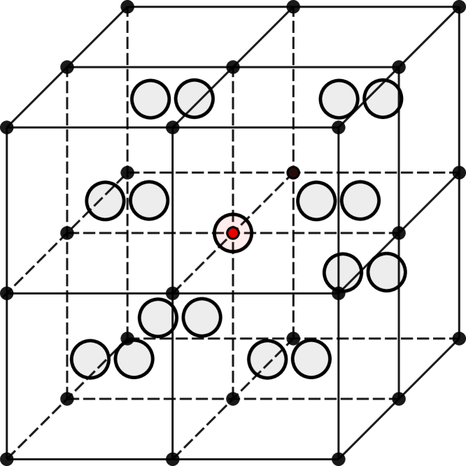
Figure 2: Macro-element distribution of degrees of freedom for ${{\mathbf{v}}}_{h}\in\bm{V}_{0,\mathrm{M}}$ and $q_{h}\in P_{\mathrm{M}}$. Small filled dots correspond to $P_{\mathrm{M}}$ and bigger opaque circles correspond to $\bm{V}_{0,\mathrm{M}}$.

3.4 Changes and limitations in the nonlinear case

One of the main differences between the linear and nonlinear case stems from the definition of the pressure $p$ as remarked in boffi2017remark (16). Consider, as an example, the strain energy function for a nearly incompressible neo-Hookean material where

$$\overline{\Psi}(\overline{\bm{C}}):=\frac{\mu}{2}\left(\mathrm{tr}(\overline{\bm{C}})-3\right),$$

with $\mu>0$ a material parameter. Then, $\bm{S}_{\mathrm{tot}}$ and $\mathbb{C}_{\mathrm{tot}}$, evaluated at $({{\mathbf{u}}}_{k},p_{k})=({{\mathbf{0}}},0)$, are given by

$$\bm{S}_{\mathrm{tot}}=\bm{0},\quad\mathbb{C}_{\mathrm{tot}}=2\mu\bm{I}\odot\bm{I}-\frac{2\mu}{3}\bm{I}\otimes\bm{I},$$

independent of the choice of $\Theta(J)$. Assuming that $\Omega:=\Omega_{0}\approx\Omega_{t}$ we obtain from Eqs. (20)–(21) the following linear system

$$2\mu\int\limits_{\Omega}\bm{\varepsilon}_{\mathrm{d}}({{\mathbf{u}}}):\bm{\varepsilon}_{\mathrm{d}}({{\mathbf{v}}})\,\mathrm{d}{{\mathbf{x}}}+\int\limits_{\Omega}p\operatorname{div}{{\mathbf{v}}}\,\mathrm{d}\bm{\mathbf{x}} =\int\limits_{\Omega}{{\mathbf{f}}}\cdot{{\mathbf{v}}}\,\mathrm{d}\bm{\mathbf{x}},$$ (44)

$$\int\limits_{\Omega}\operatorname{div}{{\mathbf{u}}}q\,\mathrm{d}\bm{\mathbf{x}}-\frac{1}{\kappa}\int\limits_{\Omega}pq\,\mathrm{d}\bm{\mathbf{x}} =0,$$ (45)

where $\bm{\varepsilon}_{\mathrm{d}}({{\mathbf{u}}}):=\bm{\varepsilon}({{\mathbf{u}}})-\frac{1}{3}\mathrm{div}({{\mathbf{u}}})\bm{I}$. While the pressure in formulation (31)–(32) is usually denoted as Herrmann pressure herrmann1965elasticity (44), above formulation (44)–(45) uses the so-called hydrostatic pressure.
The arguments to prove the inf-suf condition for this linear problem remains the same as for (31)–(32). For the extension of the inf-suf condition to the nonlinear case we already stated earlier in Eq. (27) that

$$b_{k}(q_{h},{{\mathbf{v}}}_{h})=\int\limits_{\Omega_{t,h}}q_{h}\Theta^{\prime}(J_{h})\operatorname{div}{{\mathbf{v}}}_{h}\,\mathrm{d}{{\mathbf{x}}}.$$

Here, $\Omega_{t,h}$ is the approximation of the real current configuration $\Omega_{t}$. Our conjecture is that stability of the chosen elements is given provided sufficient fine discretizations and volumetric functions $\Theta(J)$ fulfilling $\Theta^{\prime}(J)\geq 1$. However, we can not offer a rigorous proof of this, and rely on our numerical results which showed no sign of numerical instabilities.
Concerning well-posedness of (44)–(45), it was noted in boffi2017remark (16), that the coercivity on the kernel condition (25) does not hold in general, which makes the formulation with hydrostatic pressure not well-posed in general. However, it remains well-posed for strictly divergence-free finite elements or pure Dirichlet boundary conditions. This has also been observed by other authors, see khan2019 (52, 81). Even if the coercivity on the kernel condition can be shown for the hydrostatic, nearly incompressible linear elastic case this result may not transfer to the nonlinear case. Here, this condition is highly dependent on the chosen nonlinear material law and for the presented benchmark examples (Section 4) we did not observe any numerical instabilities.
For an in-depth discussion we refer the interested reader to auricchio2010importance (6, 8). A detailed discussion on Herrmann-type pressure in the nonlinear case is presented in shariff1997 (72, 73).
To show well-posedness for the special case of the presented MINI element discretizations we rely on results given in (boffi2017remark, 16, Section 4). There it is shown, that discrete coercivity on the kernel holds, provided that a rigid body mode is the only function that renders

$$a({{\mathbf{u}}}_{h},{{\mathbf{v}}}_{h}):=\int\limits_{\Omega_{h}}\bm{\varepsilon}_{d}({{\mathbf{u}}}_{h}):\bm{\varepsilon}_{d}({{\mathbf{v}}}_{h})\,\mathrm{d}{{\mathbf{x}}}$$

from (44)–(45) zero. We could obtain this result following the same procedure outlined in boffi2017remark (16) for both hexahedral and tetrahedral MINI elements. A Mathematica^TM notebook containing the computations discussed is available upon request.
In the case of the pressure-projection stabilization we will modify Equation (17) using the stabilization term (38)

$$R_{\mathrm{lower}}({{\mathbf{u}}}_{h},p_{h};\Delta q_{h}) :=b_{\mathrm{vol}}({{\mathbf{u}}}_{h};\Delta q_{h})-c(p_{h},\Delta q_{h})$$

$$-\frac{1}{\mu^{*}}s_{h}(p_{h},q_{h}).$$

Here, the stabilization parameter $\mu^{*}>0$ is supposed to be large enough and will be specifically defined for each nonlinear material considered. Note, that by modifying the definition of the lower residual, we introduced a mesh dependent perturbation of the original residual. An estimate of the consistency error caused by this is not readily available and will be the topic of future research. However, results and comparisons to benchmarks in Section 4 suggest that this error is negligible for the considered problems as long as $\mu^{\ast}$ is well-chosen. If not specified otherwise we chose

• $\mu^{\ast}=\mu$ for neo-Hookean materials and

• $\mu^{\ast}=c_{1}$ for Mooney–Rivlin materials

in the results section. For the pressure-projection stabilized equal order pair we can not transfer the results from the linear elastic case to the non-linear case, as the proof of well-posedness relies on the coercivity of $a_{k}({{\mathbf{u}}},{{\mathbf{v}}})$ which can not be concluded for this formulation. However, no convergence issues occured in the numerical examples given in Section 4.
The considerable advantage of the MINI element is that there are no modifications needed and that no additional stabilization parameters are introduced into the system.

3.5 Changes and limitations in the transient case

The equations presented in Section 2 are not yet suitable for transient simulations. To include this feature we modify the nonlinear variational problem (18) in the following way:

$$R_{\mathrm{upper}}^{\mathrm{trans}}({{\mathbf{u}}},p;\Delta{{\mathbf{v}}}) :=\rho_{0}\int\limits_{\Omega_{0}}\ddot{{{\mathbf{u}}}}\cdot\Delta{{\mathbf{v}}}\,\mathrm{d}{{\mathbf{x}}}+R_{\mathrm{upper}}({{\mathbf{u}}},p;\Delta v),$$ (46)

$$R_{\mathrm{lower}}^{\mathrm{trans}}({{\mathbf{u}}},p;\Delta q) :=R_{\mathrm{lower}}({{\mathbf{u}}},p;\Delta q).$$ (47)

For time discretization we considered a generalized-$\alpha$ method, see chung1993 (28) and also the Appendix for a short summary. Due to the selected formulation, the resulting ODE system turns out to be of degenerate hyperbolic type. Hence, we implemented a variant of the generalized-$\alpha$ method as proposed in kadapa2017 (50) and using that we did not observe any numerical issues in our simulations. Note, that other groups have proposed a different treatment of the incompressibility constraints in the case of transient problems, see rossi2016implicit (66, 71) for details.

4 Numerical examples

While benchmark cases presented in this section are fairly simple, mechanical applications often require highly resolved meshes. Thus, efficient and massively parallel solution algorithms for the linearized system of equations become an important factor to deal with the resulting computational load. After discretization, at each Newton–Raphson step a block system of the form

$$\begin{pmatrix}\bm{K}_{h}&\bm{B}_{h}^{\top}\\ \bm{B}_{h}&\bm{C}_{h}\end{pmatrix}\begin{pmatrix}\Delta{{\mathbf{u}}}\\ \Delta{{\mathbf{p}}}\end{pmatrix}=\begin{pmatrix}-\bm{\mathbf{R}}_{\mathrm{upper}}\\ -\bm{\mathbf{R}}_{\mathrm{lower}}\end{pmatrix}$$

has to be solved. In that regard, we used a generalized minimal residual method (GMRES) and efficient preconditioning based on the PCFIELDSPLIT package from the library PETSc petsc-user-ref (12) and the incorporated solver suite hypre/BoomerAMG henson2002boomeramg (43). By extending our previous work augustin2016anatomically (5) we implemented the methods in the finite element code Cardiac Arrhythmia Research Package (CARP) vigmond2008solvers (82).

4.1 Analytic solution

To verify our implementation we consider a very simple uniaxial tension test, see also (weise2014, 83, Sec. 10.1). The computational domain is described by one eighth part of a cylinder with length $L=$2\text{\,}\mathrm{mm}$$, and radius $R=$1\text{\,}\mathrm{mm}$$

$$\Omega_{\mathrm{cyl,0}}:=\left\{{{\mathbf{x}}}\in[0,L]\times{[0,R]}^{2}:y^{2}+z^{2}\leq R\right\},$$

see Figure 3. This cylinder is stretched to a length of $L+\Delta L$, with $\Delta L=$2\text{\,}\mathrm{mm}$$.

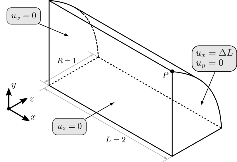
Figure 3: Analytic solution: geometry and boundary conditions.

We chose a neo-Hookean material

$$\Psi(\bm{C})=\frac{\mu}{2}\left(\mathrm{tr}(\overline{\bm{C}})-3\right)+\frac{\kappa}{2}{\ln(J)}^{2},$$

with $\mu=$7.14\text{\,}\mathrm{MPa}$$ and impose full incompressiblity, i.e., $1/\kappa=0$. For this special case, an analytic solution can be computed by

$${{\mathbf{u}}} =(tx,\Delta R(t)y,\Delta R(t)z),$$

$$p(t) =\frac{\mu}{3}\left({\left(1+\frac{t\Delta L}{L}\right)}^{2}-{\left(1+\frac{t\Delta L}{L}\right)}^{-1}\right),$$

$$\Delta R(t) ={\left(1+\frac{t\Delta L}{L}\right)}^{-\frac{1}{2}}-1,$$

where $t\in[0,1]$ corresponds to the load increment. Two meshes consisting of $5420$ points and $4617$ hexahedral or $27\,702$ tetrahedral elements were used. We performed 20 incremental load steps with respect to $\Delta L$. In Figure 4 it is shown that the results of the numerical simulations render identical results for all the chosen setups and are in perfect agreement with the exact solution plotted in blue.

(a)

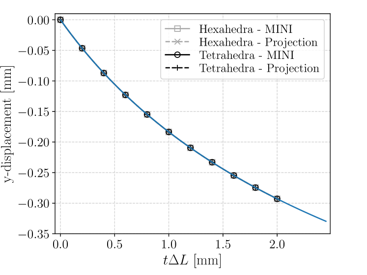
(b)

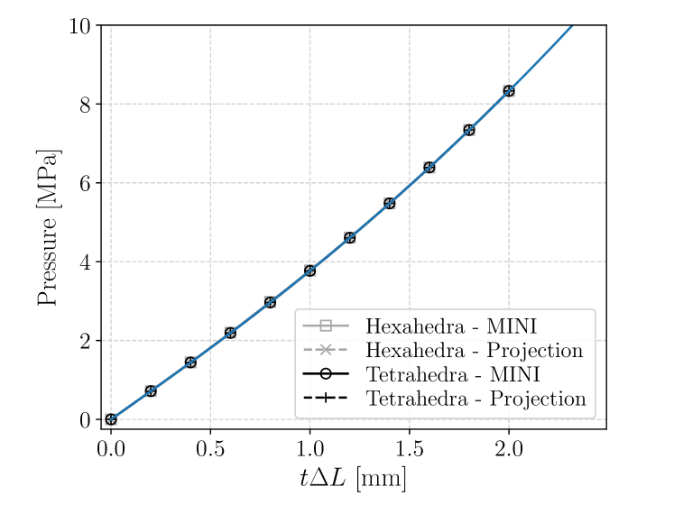
Figure 4: Analytic solution: (a) $y$-component of displacement and (b) pressure at point $P={(2,0,1)}^{\top}$. Simulation results of all proposed formulations are in perfect alignment with the analytic solution printed in blue.

4.2 Block under compression

The computational domain, studied by multiple authors, see, e.g., caylak2012stabilization (23, 58, 64), consists of a cube loaded by an applied pressure in the center of the top face; see Figure 5. A quarter of the cube is modeled, where symmetric Dirichlet boundary conditions are applied to the vertical faces and the top face is fixed in the horizontal plane.

Figure 5: Block under compression: geometry and boundary conditions.

The same neo-Hookean material model as in masud2013framework (58) is used:

$$\Psi(\bm{C}) =\frac{1}{2}\mu\left(\operatorname{tr}(\bm{C})-3\right)-\mu\ln J+\frac{\lambda}{2}{(\ln J)}^{2},$$

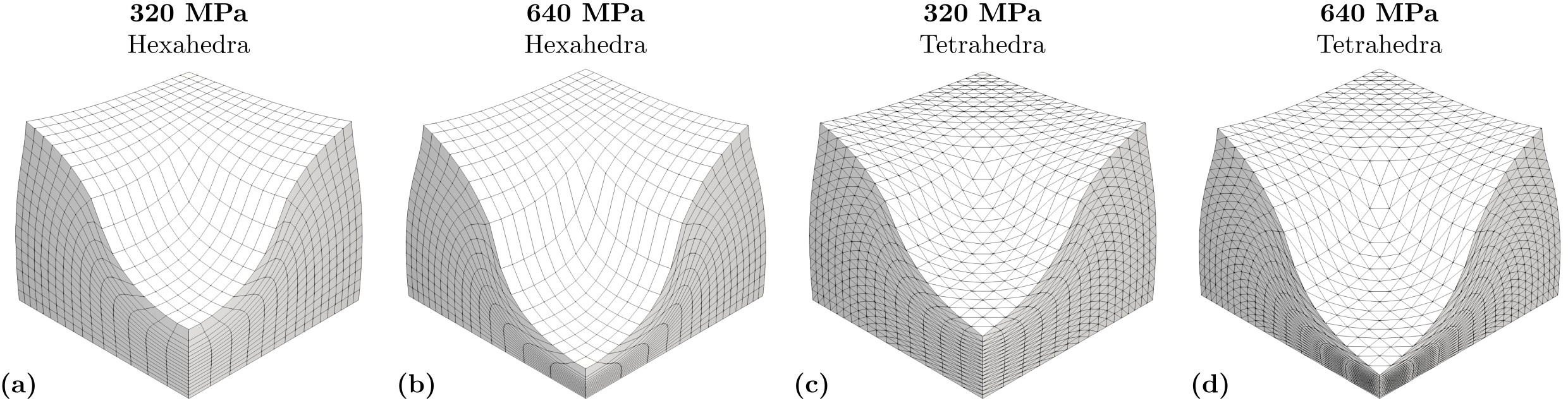
Figure 7: Block under compression: deformed meshes of hexahedral (a,b) and tetrahedral (c,d) elements for the $\ell=2$ mesh in Table 1 at load level $p=$320\text{\,}\mathrm{MPa}$$ (a,c) and load level $p=$640\text{\,}\mathrm{MPa}$$ (b,d).

with material parameters $\lambda=$400\,889.806\text{\,}\mathrm{MPa}$$, $\mu=$80.194\text{\,}\mathrm{MPa}$$. To test mesh convergence the simulations were computed on a series of uniformly refined tetrahedral and hexahedral meshes, see Table 1. Figure 7 shows the deformed meshes for the level $\ell=2$ with loads $p_{0}=$320\text{\,}\mathrm{MPa}$$ and $p_{0}=$640\text{\,}\mathrm{MPa}$$, respectively. In all cases discussed in this section we used 10 loading steps to arrive at the target pressure $p_{0}$.

Table 1: Properties of cube meshes used in Section 4.2.

Hexahedral Meshes
$\ell$	Elements	Nodes
1	$512$	$729$
2	$4096$	$4913$
3	$32\,768$	$35\,937$
4	$262\,144$	$274\,625$
5	$2\,097\,152$	$2\,146\,689$

Tetrahedral Meshes
$\ell$	Elements	Nodes
1	$3072$	$729$
2	$24\,576$	$4913$
3	$196\,608$	$35\,937$
4	$1\,572\,864$	$274\,625$
5	$12\,582\,912$	$2\,146\,689$

As a measure of the compression level the vertical displacement of the node at the center of the top surface, i.e. the edge point A of the quarter of the cube, is plotted in Figure 6. Small discrepancies can be attributed to differences in the meshes for tetrahedral and hexahedral grids, however, the different stabilization techniques yield almost the same results for finer grids. Note, that the displacements at the edge point A obtained using the simple $\mathbb{Q}_{1}-\mathbb{P}_{0}$ hexahedral and $\mathbb{P}_{1}-\mathbb{P}_{0}$ tetrahedral elements seem to be in a similar range compared to the other approaches. The overall displacement field, however, was totally inaccurate rendering $\mathbb{Q}_{1}-\mathbb{P}_{0}$ and $\mathbb{P}_{1}-\mathbb{P}_{0}$ elements an inadequate choice for this benchmark problem. The solution for Taylor–Hood ($\mathbb{P}_{2}-\mathbb{P}_{1}$) tetrahedral elements was obtained using the FEniCS project alnaes2015fenics (2). Here, as a linear solver, we used a GMRES solver with preconditioning similar to the MINI and projection-based approach, see first paragraph of Section 4. The PCFIELDSPLIT and hypre/BoomerAMG settings were slightly adapted to optimize computational performance for quadratic ansatz functions. We comparing simulations with about the same number of degrees of freedom, not accuracy as, e.g., in chamberland2010comparison (25). For coarser grids computational times were in the same time range for all approaches; see, e.g., the cases with approximately $10^{6}$ degrees of freedom and target pressure of $p_{0}=$320\text{\,}\mathrm{mmHg}$$ in Table 2(a). For the simulations with the finest grids with approximately $10^{7}$ degrees of freedom, however, we could not find a setting for the Taylor–Hood elements that was competitive to MINI and pressure-projection stabilizations. The computational times to arrive at the target pressure of $p_{0}=$320\text{\,}\mathrm{mmHg}$$ using 192 cores on ARCHER, UK were about 10 times higher for Taylor–Hood elements using FEniCS, see Table 2(b). We attribute that to a higher communication load and higher memory requirements of the Taylor–Hood elements: memory to store the block stiffness matrices was approximately $2.5$ times higher for Taylor–Hood elements compared to MINI and projection-stabilization approaches (measured using the MatGetInfo function provided by PETSc). Note, that although we used the same linear solvers, the time comparisons are not totally just as results were obtained using two different finite element solvers, CARP and FEniCS. Note also, that timings are usually very problem dependent and for this block under compression benchmark high accuracy was already achieved with coarse grids for hexahedral and Taylor–Hood discretizations.
For a further analysis regarding computational costs of the MINI element and the pressure-projection stabilization, see Section 4.4.

Table 2: Block under compression: Comparison of computational times for different discretizations. Timings were obtained using (a) 48 cores and (b) 192 cores on ARCHER, UK. Coarser grids, see Table 1, are used for Taylor–Hood elements $\mathbb{P}_{2}-\mathbb{P}_{1}$ to compare computational times for a similar number of degrees of freedom (DOF).

(a)
Discretization Grid DOF Tet. Hex. Projection $\ell=4$ 1.098 Mio. $330\text{\,}\mathrm{s}$ $438\text{\,}\mathrm{s}$ MINI $\ell=4$ 1.098 Mio. $873\text{\,}\mathrm{s}$ $655\text{\,}\mathrm{s}$ $\mathbb{P}_{2}-\mathbb{P}_{1}$ $\ell=3$ 0.860 Mio. $1202\text{\,}\mathrm{s}$ –
(b)
Discretization Grid DOF Tet. Hex. Projection $\ell=5$ 8.587 Mio. $2488\text{\,}\mathrm{s}$ $2192\text{\,}\mathrm{s}$ MINI $\ell=5$ 8.587 Mio. $3505\text{\,}\mathrm{s}$ $4640\text{\,}\mathrm{s}$ $\mathbb{P}_{2}-\mathbb{P}_{1}$ $\ell=4$ 6.715 Mio. $27\,154\text{\,}\mathrm{s}$ –

In Figure 8 the hydrostatic pressure is plotted for the MINI element and the projection-based stabilization. These results are very smooth in all cases and agree well with those published in caylak2012stabilization (23, 35, 58, 64).

(a)

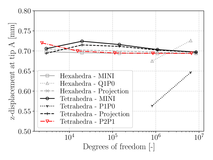
(b)

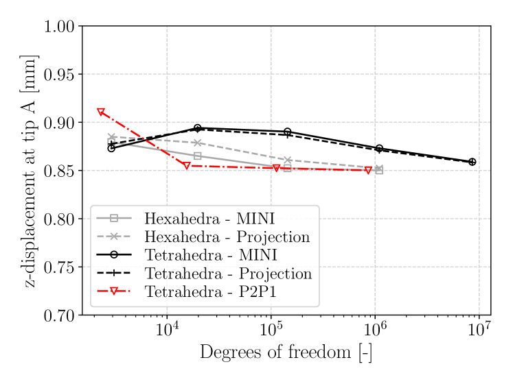
Figure 6: Block under compression: vertical displacement at point A versus number of degrees of freedom in a logarithmic scale at load level (a) $p_{0}=$320\text{\,}\mathrm{MPa}$$ and (b) $p_{0}=$640\text{\,}\mathrm{MPa}$$. Results for the MINI element and the pressure-projection stabilization are compared to classical choices of elements, i.e., $\mathbb{Q}_{1}-\mathbb{P}_{0}$ hexahedral elements, $\mathbb{P}_{1}-\mathbb{P}_{0}$ tetrahedral elements, and Taylor–Hood ($\mathbb{P}_{2}-\mathbb{P}_{1}$) tetrahedral elements. For case (b) the choice of $\mathbb{Q}_{1}-\mathbb{P}_{0}$ and $\mathbb{P}_{1}-\mathbb{P}_{0}$ elements did not give reasonable results and were thus omitted.

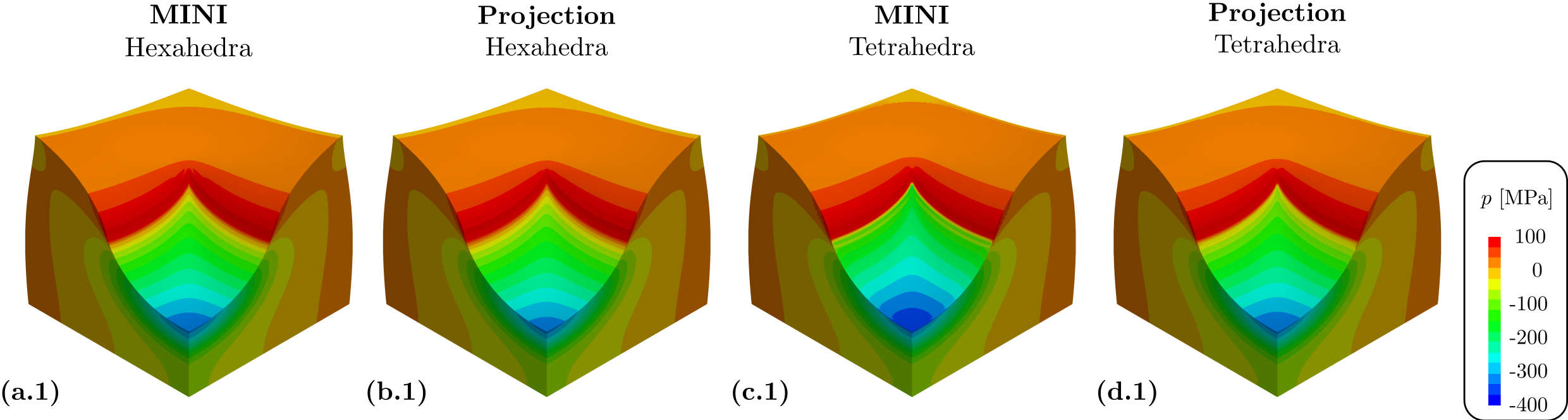
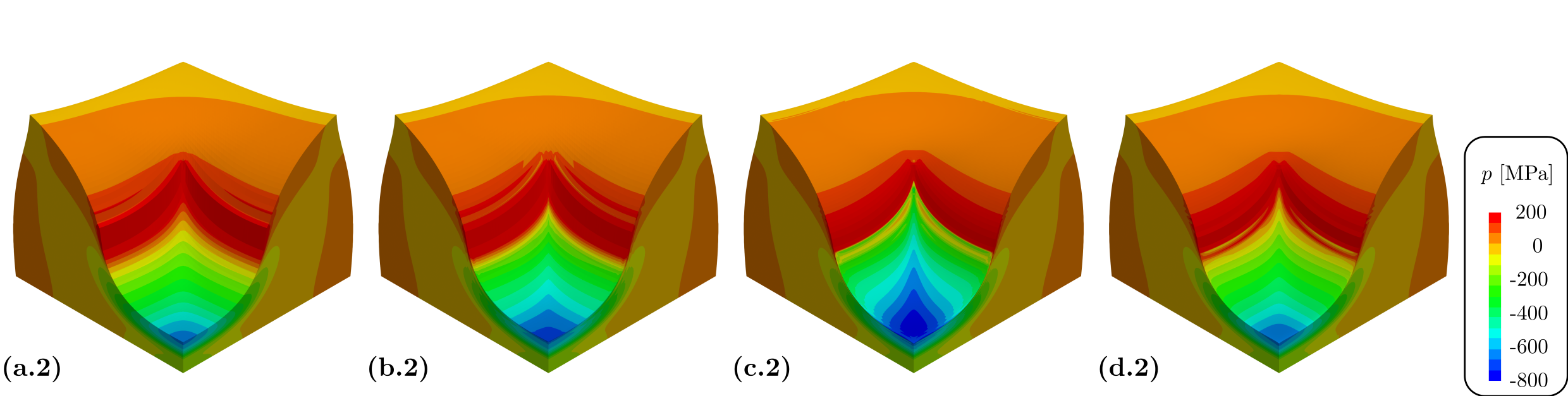
Figure 8: Block under compression: comparison of hexahedral (a,b) and tetrahedral (c,d) elements with bubble-based (a,c) and projection-based (b,d) stabilization. Shown is the pressure contour on the deformed mesh at load level $p=$320\text{\,}\mathrm{MPa}$$ in the first row and $p=$640\text{\,}\mathrm{MPa}$$ in the second row.

4.3 Cook-type cantilever problem

In this section, we analyze the same Cook-type cantilever beam problem presented in bonet2015computational (17, 69), see also Figure 9. Displacements at the plane $x=$0\text{\,}\mathrm{mm}$$ are fixed. At the plane $x=$48\text{\,}\mathrm{mm}$$ a parabolic load, which takes its maximum at $t_{0}=$300\text{\,}\mathrm{kPa}$$, is applied. Note, that this in-plane shear force in y-direction is considered as a dead load in the deformation process.

Figure 9: Cook-type cantilever problem: geometry and boundary conditions.

To compare to results in schroeder2011new (69) the same isotropic strain energy function was chosen

$$\Psi^{\mathrm{iso}}(\bm{C})=c_{1}{(\operatorname{tr}\bm{C})}^{2}+c_{2}{({(\operatorname{tr}\bm{C})}^{2}-\operatorname{tr}(\bm{C}^{2}))}^{2}-\gamma\ln(J),$$

with material properties $c_{1}=$21\text{\,}\mathrm{kPa}$$, $c_{2}=$42\text{\,}\mathrm{kPa}$$, and $\gamma=12c_{1}+24c_{2}$ to satisfy the condition of a stress-free reference geometry.

We chose a fully incompressible material, hence,

$$\Psi^{\mathrm{vol}}(\bm{C})=\frac{\kappa}{2}{\left(J-1\right)}^{2},$$

with $1/\kappa=0$. First, mesh convergence with respect to resulting displacements is analyzed for the tetrahedral and hexahedral meshes with discretization details given in Table 3.

Table 3: Properties of cantilever meshes used in Section 4.3.

Hexahedral Meshes
$\ell$	Elements	Nodes
1	$324$	$500$
2	$2592$	$3249$
3	$20\,736$	$23\,273$
4	$165\,888$	$175\,857$

Tetrahedral Meshes
$\ell$	Elements	Nodes
1	$1944$	$500$
2	$15\,552$	$3249$
3	$124\,416$	$23\,273$
4	$995\,328$	$175\,857$

Displacements $u_{x}$, $u_{y}$, and $u_{z}$ at point $\mathbf{C}$ are shown in Figure 10. The proposed stabilization techniques give comparable displacements in all three directions and also match results published in bonet2015computational (17, 69). Mesh convergence can also be observed for the stresses $\sigma_{xx}$ at point $\mathbf{A}$ and $\mathbf{B}$ and $\sigma_{yy}$ at point $\mathbf{B}$, see Figure 11. Again, results match well those presented in bonet2015computational (17, 69). Small discrepancies can be attributed to the fully incompressible formulation used in our work and differences in grid construction.

In Figure 12 and Figure 13(a) the distribution of $J=\det(\bm{F})$ is shown to provide an estimate of how accurately the incompressibility constraint is fulfilled by the proposed stabilization techniques. For most parts of the computational domains the values of $J$ are close to $1$, however, hexahedral meshes and here in particular the MINI element maintain the condition of $J\approx 1$ more accurately on the element level. Note, that for all discretizations the overall volume of the cantilever remained unchanged at $14\,400\text{\,}{\mathrm{mm}}^{3}$, rendering the material fully incompressible on the domain level.

Figure 13 gives a comparison of several computed values in the deformed configuration of Cook’s cantilever for the finest grids ($\ell=4$). Slight pressure oscillations in Figure 13(b) on the domain boundary for the MINI element are to be expected, see soulaimani1987 (74); this also affects the distribution of $J$ in Figure 13(a). A similar checkerboard pattern is present for the projection based stabilization.

In the third row of Figure 13 we compare the stresses $\sigma_{xx}$ for the different stabilization techniques. We can observe slight oscillations for the the projection-based approach, whereas the MINI element gives a smoother solution. Compared to results in (schroeder2011new, 69, Figure 10) the $\sigma_{xx}$ stresses have a similar contour but are slightly higher. As before, we attribute that to the fully incompressible formulation in our paper compared to the quasi-incompressible formulation in schroeder2011new (69).

(a)

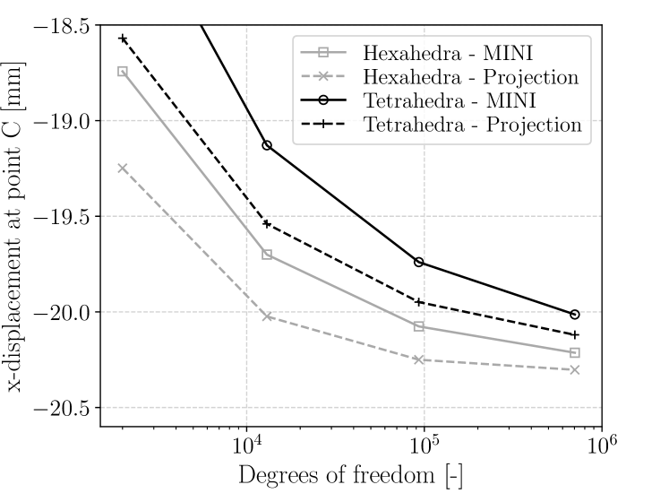
(b)

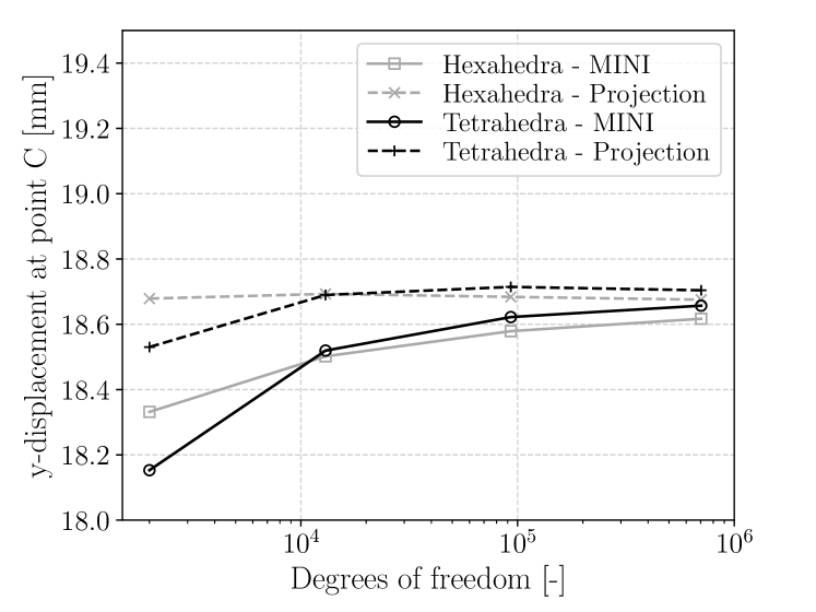
(c)

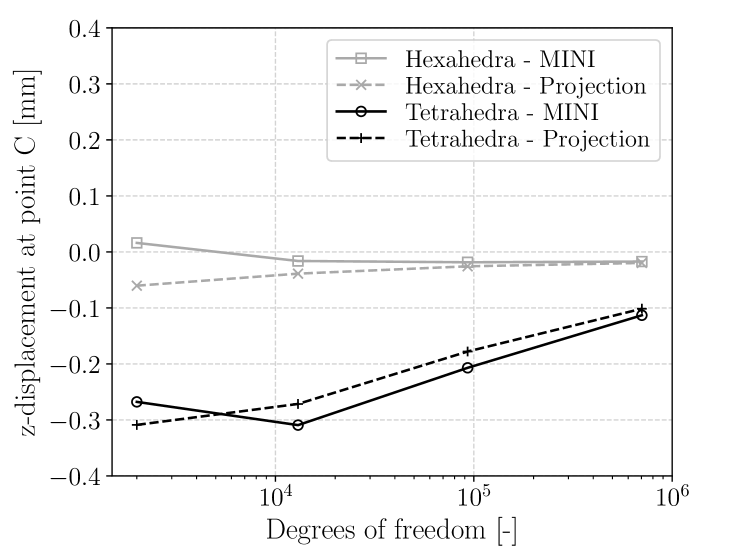
Figure 10: Cook-type cantilever problem: displacements $u_{x}$, $u_{y}$, and $u_{z}$ at point C versus the number of degrees of freedom in a logarithmic scale using the fully incompressible formulation.

(a)

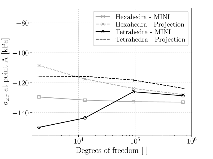
(b)

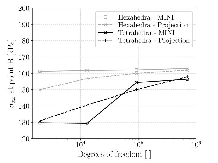
(c)

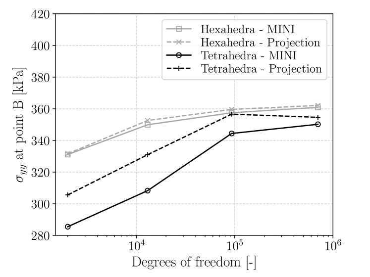
Figure 11: Cook-type cantilever problem: stresses $\sigma_{xx}$ at (left) point A and (middle) point B and $\sigma_{yy}$ at (right) point B versus the number of degrees of freedom in a logarithmic scale using the fully incompressible formulation.

(a)

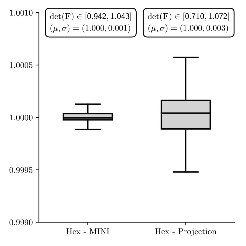
(b)

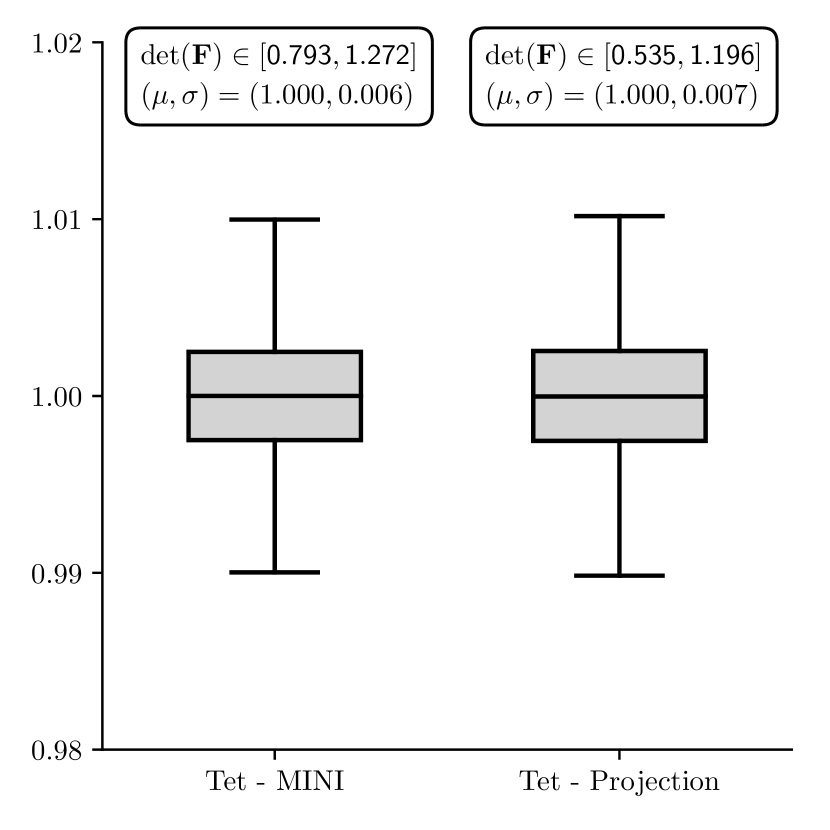
Figure 12: Cook-type cantilever problem: boxplots showing the distribution of $J=\det(\bm{F})$ for (a) hexahedral and (b) tetrahedral elements. Additionally, the minimal and maximal value, as well as the mean ($\mu$) and the standard deviation ($\sigma$) is given for each setting.

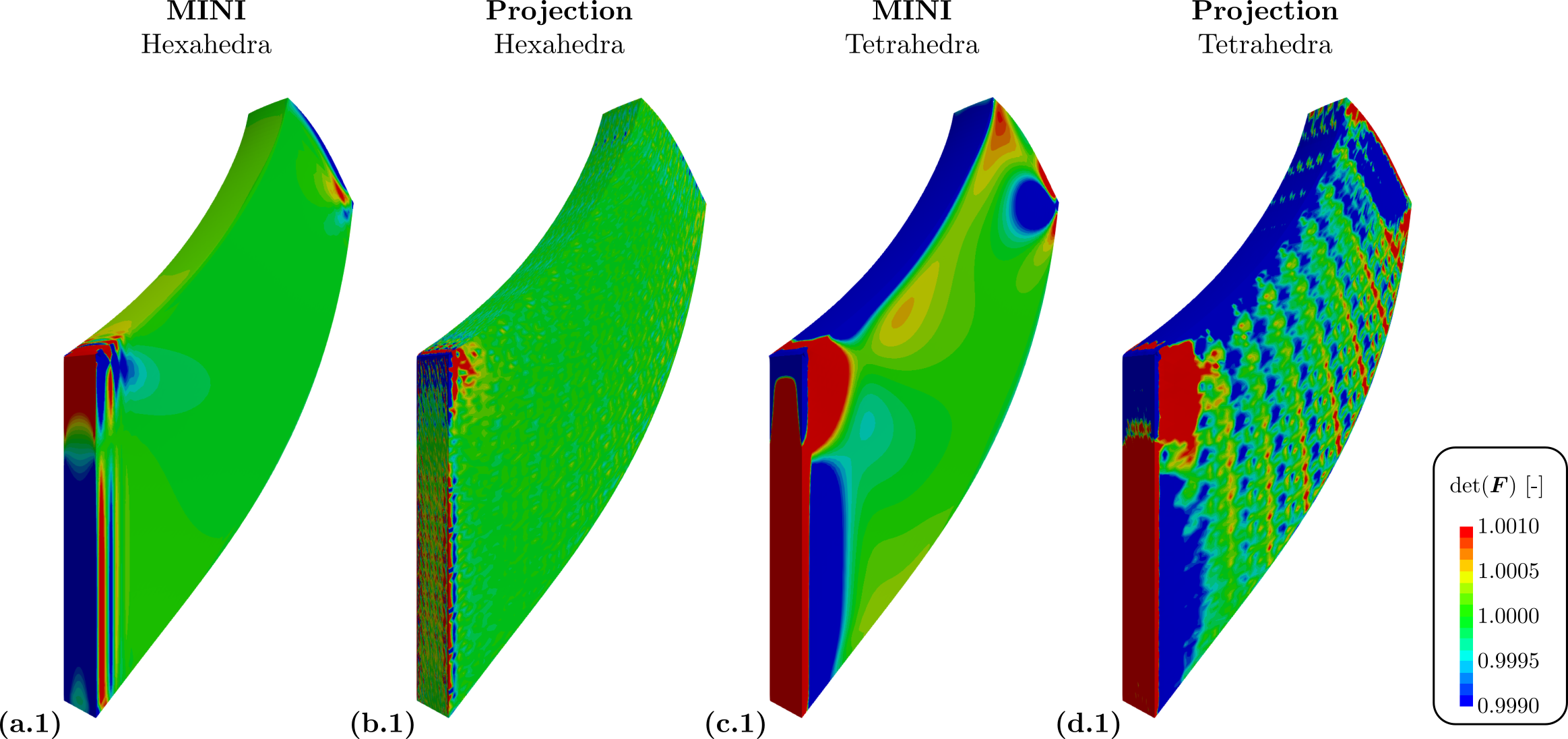
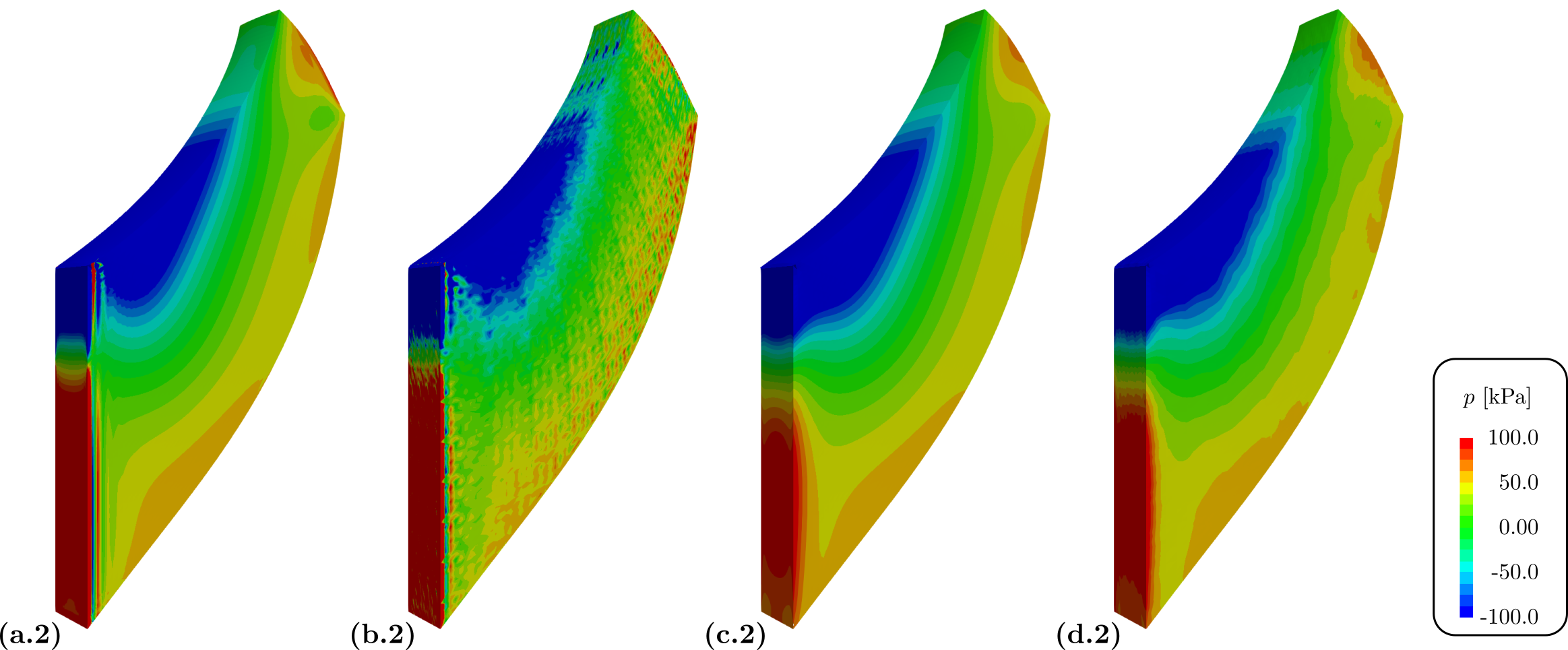
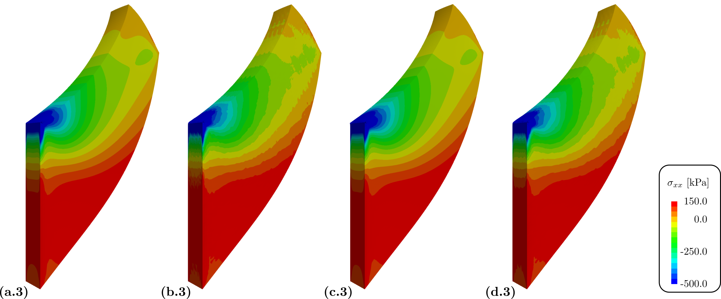
Figure 13: Cook-type cantilever problem: comparison of hexahedral (a,c) and tetrahedral (b,d) elements with bubble-based (a,b) and projection-based (c,d) stabilization. Shown is the distribution of $J=\det(\bm{F})$ (first row); distribution of the hydrostatic pressure $p$ (second row) in $\mathrm{kPa}$; and the distribution of the stress $\sigma_{xx}$ (third row) in $\mathrm{kPa}$ for the fully incompressible formulation.

4.4 Twisting column test

Finally, we show the applicability of our stabilization techniques for the transient problem of a twisting column aguirre2014vertex (1, 40, 71). The initial configuration of the geometry is depicted in Figure 14. There is no load prescribed and the column is restrained against motion at its base. A twisting motion is applied to the domain by means of the following initial condition on the velocity

$${{\mathbf{v}}}({{\mathbf{x}}},0)={{\mathbf{v}}}(x,y,z,0)=100\sin\left(\frac{\pi y}{12}\right){\left(z,0,-x\right)}^{\top}$\mathrm{m}\mathrm{/}\mathrm{s}$,$$

for $y\in\left[0,6\right]$\mathrm{m}$$. To avoid symmetries in the problem the column is rotated about the $z$-axes by an angle of $\theta=$5.2\text{\,}\mathrm{\SIUnitSymbolDegree}$$.

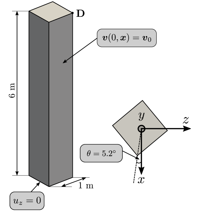
Figure 14: Twisting column test: geometry and boundary conditions.

We chose the neo-Hookean strain-energy

$$\Psi(\bm{C})=\frac{\mu}{2}\left(\mathrm{tr}(\overline{\bm{C}})-3\right)+\frac{\kappa}{2}{(J-1)}^{2},$$

with parameters $\mu=$5704.7\text{\,}\mathrm{kPa}$$ and $\kappa=$283\,333\text{\,}\mathrm{k}\mathrm{P}\mathrm{a}$$ for the nearly incompressible and $1/\kappa=0$ for the truly incompressible case. For the results presented, we considered hexahedral and tetrahedral meshes with five levels of refinement, respectively; for discretization details of the column meshes see Table 4.

Table 4: Properties of column meshes used in Section 4.4.

Hexahedral Meshes
$\ell$	Elements	Nodes
1	$48$	$117$
2	$384$	$625$
3	$3072$	$3969$
4	$24\,576$	$28\,033$
5	$196\,608$	$210\,177$

Tetrahedral Meshes
$\ell$	Elements	Nodes
1	$240$	$117$
2	$1920$	$625$
3	$15\,360$	$3969$
4	$122\,880$	$28\,033$
5	$983\,040$	$210\,177$

In Figure 15, mesh convergence with respect to tip displacement $(u_{x},u_{y},u_{z})$ at point D is analyzed. While differences at lower levels of refinement $\ell=1,2$ are severe, the displacements converge for higher levels of refinement $\ell=3,4,5$. For finer grids the curves for tetrahedral and hexahedral elements are almost indistinguishable, see also Figure 16, and the results are in good agreement with those presented in scovazzi2016simple (71). While this figure was produced using MINI elements we also observed a similar behavior of mesh convergence for the projection-based stabilization. In fact, for the finest grid, all the proposed stabilization techniques and elements gave virtually identical results, see Figure 16. Further, as already observed by scovazzi2016simple (71), the fully and nearly incompressible formulations gave almost identical deformations, see Figure 17.

In Figure 18 stress $\sigma_{yy}$ and pressure $p$ contours are plotted on the deformed configuration for the incompressible case at time instant $t=$0.3\text{\,}\mathrm{s}$$. Minor pressure oscillations can be observed for tetrahedral elements. Again, results match well those presented in (scovazzi2016simple, 71, Figure 22).

Finally, in Figure 19, we compare the magnitude of velocity and acceleration at time instant $t=$0.3\text{\,}\mathrm{s}$$. Results for these variables are very smooth and hardly distinguishable for all the different approaches.

The computational costs for this nonlinear elasticity problem were significant due to the required solution of a saddle-point problem in each Newton step and a large number of time steps. However, this challenge can be addressed by using a massively parallel iterative solving method and exploiting potential of modern HPC hardware. The most expensive simulations were the fully incompressible cases for the finest grids with a total of $840\,708$ degrees of freedom and $400$ time steps. These computations were executed at the national HPC computing facility ARCHER in the United Kingdom using $96$ cores. Computational times were as follows: $239\text{\,}\min$ for tetrahedral meshes and projection-based stabilization; $283\text{\,}\min$ for tetrahedral meshes and MINI elements; $449\text{\,}\min$ for hexahedral meshes and projection-based stabilization; and $752.5\text{\,}\min$ for hexahedral meshes and MINI elements. Simulation times for nearly incompressible problems were lower, ranging from $177$ to $492\text{\,}\min$. This is due to the additional matrix on the lower-right side of the block stiffness matrix which led to a smaller number of linear iterations. Simulations with hexahedral meshes were, in general, computationally more expensive compared to simulations with tetrahedral grids; the reason beeing mainly a higher number of linear iterations. Computational burden for MINI elements was larger due to higher matrix assembly times. However, this assembly time is highly scalable as there is almost no communication cost involved in this process.

(A) Mesh convergence for hexahedral elements:

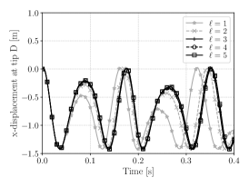
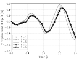
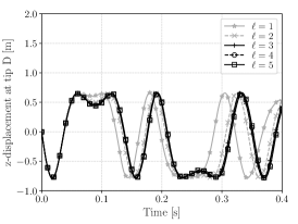
(B) Mesh convergence for tetrahedrnts:

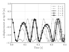
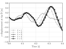
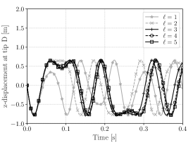
Figure 15: Twisting column test: mesh convergence for (A) hexahedral and (B) tetrahedral elements. Shown are displacements $u_{x}$, $u_{y}$, and $u_{z}$ at tip D versus time. For experiments depicted the incompressible formulation with MINI elements was chosen. At finer levels of refinement $\ell=3,4,5$ (in black) results converge to a solution for each displacement direction.

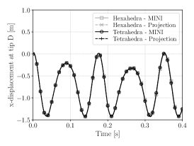
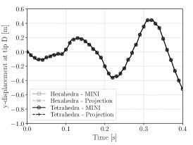
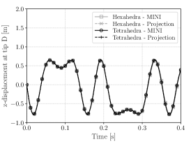
Figure 16: Twisting column test: comparison of stabilization techniques for the finest grids ($\ell=5$). Shown are displacements $u_{x}$, $u_{y}$, and $u_{z}$ at tip D versus time. Both MINI elements (dashed line) and projection-based stabilization (dashed lines) render almost identical results for hexahedral (in gray) and tetrahedral elements (in black).

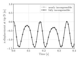
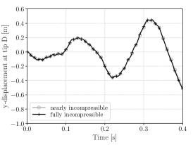
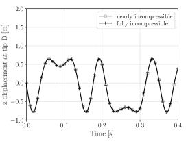
Figure 17: Twisting column test: comparison of nearly and fully incompressible formulation for the finest tetrahedral grids ($\ell=5$) and MINI elements. Displacements $u_{x}$, $u_{y}$, and $u_{z}$ are almost identical for the whole simulation duration of $0.4\text{\,}\mathrm{s}$.

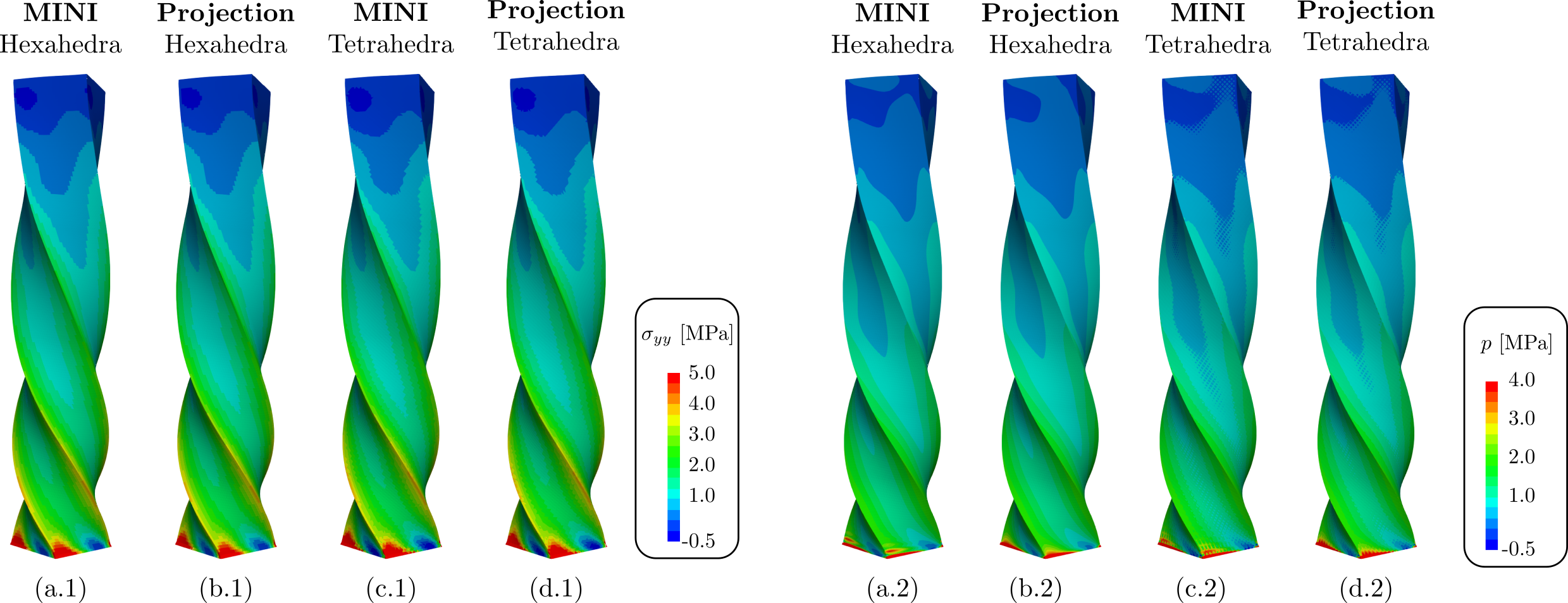
Figure 18: Twisting column test: (a) stress $\sigma_{yy}$ and (b) hydrostatic pressure $p$ contours at time instant $t=$0.3\text{\,}\mathrm{s}$$ for the different grids and stabilization techniques.

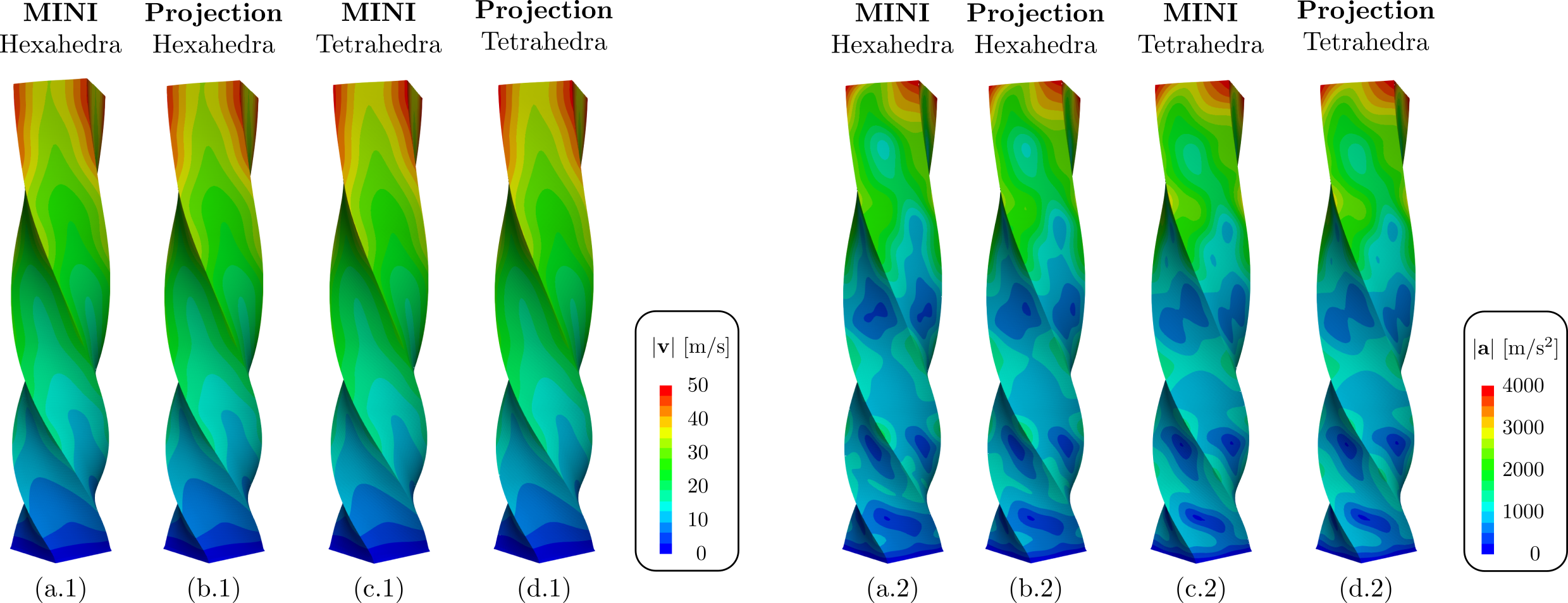
Figure 19: Twisting column test: magnitude of (a) velocity ${{\mathbf{v}}}$ and (b) acceleration ${{\mathbf{a}}}$ at time instant $t=$0.3\text{\,}\mathrm{s}$$ for the different grids and stabilization techniques.

5 Conclusion

In this study we described methodology for modeling nearly and fully incompressible solid mechanics for a large variety of different scenarios. A stable MINI element was presented which can serve as an excellent choice for applied problems where the use of higher order element types is not desired, e.g., due to fitting accuracy of the problem domain. We also proposed an easily implementable and computationally cheap technique based on a local pressure projection. Both approaches can be applied to stationary as well as transient problems without modifications and perform excellent with both hexahedral and tetrahedral grids. Both approaches allow a straightforward inclusion in combination with existing finite element codes since all required implementations are purely on the element level and are well-suited for simple single-core simulations as well as HPC computing. Numerical results demonstrate the robustness of the formulations, exhibiting a great accuracy for selected benchmark problems from the literature.

While the proposed projection method works well for relatively stiff materials as considered in this paper, the setting of the parameter $\mu^{\ast}$ has to be adjusted for soft materials such as biological tissues. A further limitation is that both formulations render the need of solving a block system, which is computationally more demanding and suitable preconditioning is not trivial. However, the MINI element approach can be used without further tweaking of artificial stabilization coefficients and preliminary results suggested robustness, even for very soft materials. Consistent linearization as presented ensures that quadratic convergence of the Newton–Raphson algorithm was achieved for all the problems considered. Note that all computations for forming the tangent matrices and also the right hand side residual vectors are kept local to each element. This benefits scaling properties of parallel codes and also enables seamless implementation in standard finite element software.

The excellent performance of the methods along with their high versatility ensure that this framework serves as a solid platform for simulating nearly and fully incompressible phenomena in stationary and transient solid mechanics. In future studies, we plan to extend the formulation to anisotropic materials with stiff fibers as they appear for example in the simulation of cardiac tissue and arterial walls.

Appendix

Generalized-$\alpha$ time integration

After spatial discretization of (46)–(47) we get the following degenerate hyperbolic system

$$\rho_{0}\bm{M}_{h}\ddot{{{\mathbf{u}}}}(t)+\bm{C}_{h}\dot{{{\mathbf{u}}}}(t)+\bm{\mathbf{R}}_{\mathrm{upper}}({{\mathbf{u}}}(t),{{\mathbf{p}}}(t)) ={{\mathbf{0}}},$$

$$\bm{\mathbf{R}}_{\mathrm{lower}}({{\mathbf{u}}}(t),{{\mathbf{p}}}(t)) ={{\mathbf{0}}},$$

$${{\mathbf{u}}}(0) ={{\mathbf{u}}}_{0},$$

$$\dot{{{\mathbf{u}}}}(0) ={{\mathbf{u}}}_{0},$$

where $\bm{M}_{h}$ denotes the mass matrix; $\bm{C}_{h}$ denotes an optional damping matrix; $\ddot{{{\mathbf{u}}}}(t)$ denote the unknown nodal accelerations; $\dot{{{\mathbf{u}}}}(t)$ denote the unknown nodal velocities; ${{\mathbf{u}}}(t)$ denote the unknown nodal displacements; and ${{\mathbf{p}}}(t)$ denote the unknown nodal pressure values. We will use the modified generalized-$\alpha$ method proposed in kadapa2017 (50). To this end we introduce the auxiliary velocity ${{\mathbf{v}}}=\dot{{{\mathbf{u}}}}$. Then, applying the standard generalized-$\alpha$ integrator from chung1993 (28) we obtain

$$\bm{M}_{h}\dot{{{\mathbf{u}}}}_{n+\alpha_{\mathrm{m}}}-\bm{M}_{h}{{\mathbf{v}}}_{n+\alpha_{\mathrm{f}}} ={{\mathbf{0}}},$$ (48)

$$\rho_{0}\bm{M}_{h}\dot{{{\mathbf{v}}}}_{n+\alpha_{\mathrm{m}}}+\bm{C}_{h}{{\mathbf{v}}}_{n+\alpha_{\mathrm{f}}}+\bm{\mathbf{R}}_{\mathrm{upper}}^{n+\alpha_{\mathrm{f}}} ={{\mathbf{0}}},$$ (49)

$$\bm{\mathbf{R}}_{\mathrm{lower}}^{n+\alpha_{\mathrm{f}}} ={{\mathbf{0}}},$$ (50)

where

$$\bm{\mathbf{R}}_{\mathrm{upper}}^{n+\alpha_{\mathrm{f}}} :=\alpha_{\mathrm{f}}\bm{\mathbf{R}}_{\mathrm{upper}}({{\mathbf{u}}}_{n+1},{{\mathbf{p}}}_{n+1}),$$

$$+(1-\alpha_{\mathrm{f}})\bm{\mathbf{R}}_{\mathrm{upper}}({{\mathbf{u}}}_{n},{{\mathbf{p}}}_{n}),$$

$$\bm{\mathbf{R}}_{\mathrm{lower}}^{n+\alpha_{\mathrm{f}}} :=\alpha_{\mathrm{f}}\bm{\mathbf{R}}_{\mathrm{lower}}({{\mathbf{u}}}_{n+1},{{\mathbf{p}}}_{n+1}),$$

$$+(1-\alpha_{\mathrm{f}})\bm{\mathbf{R}}_{\mathrm{lower}}({{\mathbf{d}}}_{n},{{\mathbf{p}}}_{n}),$$

and

$$\dot{{{\mathbf{u}}}}_{n+\alpha_{\mathrm{m}}} :=\alpha_{\mathrm{m}}\dot{{{\mathbf{u}}}}_{n+1}+(1-\alpha_{\mathrm{m}})\dot{{{\mathbf{u}}}}_{n},$$ (51)

$$\dot{{{\mathbf{v}}}}_{n+\alpha_{\mathrm{m}}} :=\alpha_{\mathrm{m}}\dot{{{\mathbf{v}}}}_{n+1}+(1-\alpha_{\mathrm{m}})\dot{{{\mathbf{v}}}}_{n},$$ (52)

$${{\mathbf{v}}}_{n+\alpha_{\mathrm{f}}} :=\alpha_{\mathrm{f}}\ {{\mathbf{v}}}_{n+1}+(1-\alpha_{\mathrm{f}})\ {{\mathbf{v}}}_{n}.$$ (53)

Moreover, we employ Newmark’s approximations, newmark85method (61),

$$\dot{{{\mathbf{u}}}}_{n+1} =\frac{1}{\gamma\Delta t}\left({{\mathbf{u}}}_{n+1}-{{\mathbf{u}}}_{n}\right)+\frac{\gamma-1}{\gamma}\dot{{{\mathbf{u}}}}_{n},$$ (54)

$${{\mathbf{v}}}_{n+1} =\frac{1}{\gamma\Delta t}\left({{\mathbf{v}}}_{n+1}-{{\mathbf{v}}}_{n}\right)+\frac{\gamma-1}{\gamma}\dot{{{\mathbf{v}}}}_{n}$$ (55)

Using (48) we observe

$$\dot{{{\mathbf{u}}}}_{n+\alpha_{\mathrm{m}}}={{\mathbf{v}}}_{n+\alpha_{\mathrm{f}}}$$

and combining this with (49)–(55) we conclude

$${{\mathbf{v}}}_{n+1} =\frac{\alpha_{\mathrm{m}}}{\alpha_{\mathrm{f}}\gamma\Delta t}\left({{\mathbf{u}}}_{n+1}-{{\mathbf{u}}}_{n}\right)+\frac{\gamma-\alpha_{\mathrm{m}}}{\gamma\alpha_{\mathrm{f}}}\dot{{{\mathbf{u}}}}_{n}+\frac{\alpha_{\mathrm{f}}-1}{\alpha_{\mathrm{f}}}{{\mathbf{v}}}_{n},$$

$$\dot{{{\mathbf{v}}}}_{n+1} =\frac{\alpha_{\mathrm{m}}}{\alpha_{\mathrm{f}}\gamma^{2}\Delta t^{2}}\left({{\mathbf{u}}}_{n+1}-{{\mathbf{u}}}_{n}\right)-\frac{1}{\alpha_{\mathrm{f}}\gamma\Delta t}{{\mathbf{v}}}_{n}+\frac{\gamma-1}{\gamma}\dot{{{\mathbf{v}}}}_{n}$$

$$+\frac{\gamma-\alpha_{\mathrm{m}}}{\alpha_{\mathrm{f}}\gamma^{2}\Delta t}\dot{{{\mathbf{u}}}}_{n}.$$

Thus, a dependence of ${{\mathbf{v}}}_{n+1}$ and $\dot{{{\mathbf{v}}}}_{n+1}$ on ${{\mathbf{u}}}_{n+1}$ can be established. Having this the unknown values ${{\mathbf{u}}}_{n+1},{{\mathbf{p}}}_{n+1}$ can be computed with the Newton–Raphson method. Based on kadapa2017 (50) we set the parameters depending only on $\rho_{\infty}\in[0,1)$ by

$$\alpha_{\mathrm{f}} :=\frac{1}{1+\rho_{\infty}},$$

$$\alpha_{\mathrm{m}} :=\frac{3-\rho_{\infty}}{2(1+\rho_{\infty})},$$

$$\gamma :=\frac{1}{2}+\alpha_{\mathrm{m}}-\alpha_{\mathrm{f}}.$$

In all our simulations we used a value of $\rho_{\infty}=0.5$.

Remark on the implementation of the pressure-projection stabilized equal order pair

Considering the bilinear form $s_{h}(p_{h},q_{h})$ defined in (38) we can rewrite this with a simple calculation into

$$s_{h}(p_{h},q_{h}):=\sum_{l=1}^{n_{\mathrm{el}}}\left(\int\limits_{K_{l}}p_{h}q_{h}\,\mathrm{d}{{\mathbf{x}}}-\frac{1}{\lvert\tau_{l}\rvert}\int\limits_{K_{l}}p_{h}\,\mathrm{d}{{\mathbf{x}}}\int\limits_{K_{l}}q_{h}\,\mathrm{d}{{\mathbf{x}}}\right).$$

Denoting by $\{\phi_{i}\}_{i=1}^{n}$ the chosen ansatz functions the element contribution for an arbitrary element $K$ to the matrix $\bm{C}_{h}$ is given by

$$\int\limits_{K}\phi_{i}\phi_{j}\,\mathrm{d}{{\mathbf{x}}}-\frac{1}{\lvert K\rvert}\int\limits_{K}\phi_{i}\,\mathrm{d}{{\mathbf{x}}}\int\limits_{K}\phi_{j}\,\mathrm{d}{{\mathbf{x}}}.$$

This corresponds to an element mass matrix minus a rank-one correction.

Static condensation

For completeness we provide a summary for the static condensation used for the MINI element. Consider a finite element $K\in\mathcal{T}_{h}$ with a local ordering of the unknowns ${{\mathbf{u}}}$

$${{\mathbf{u}}}=\left(u_{x}^{1},u_{y}^{1},u_{z}^{1},\ldots,u_{x}^{\mathrm{ndofs}_{N}},u_{y}^{\mathrm{ndofs}_{\mathrm{N}}},u_{z}^{\mathrm{ndofs}_{\mathrm{N}}},\right.\\ \left.u_{x,\mathrm{B}}^{1},u_{y,\mathrm{B}}^{1},u_{z,\mathrm{B}}^{1},\ldots,u_{x,\mathrm{B}}^{\mathrm{ndofs}_{\mathrm{B}}},u_{y,\mathrm{B}}^{\mathrm{ndofs}_{\mathrm{B}}},u_{z,\mathrm{B}}^{\mathrm{ndofs}_{\mathrm{B}}}\right)$$

and ${{\mathbf{p}}}$ as

$${{\mathbf{p}}}=\left(p^{1},p^{2},\ldots,p^{\mathrm{ndofs}_{\mathrm{N}}}\right).$$

Here, $\mathrm{ndofs}_{\mathrm{N}}$ corresponds to the nodal degrees of freedom per element and $\mathrm{ndofs}_{\mathrm{B}}$ to the bubble degrees of freedom (one for tetrahedral elements and two for hexahedral elements). Then the element contribution to the global saddle-point system can be written as

$$\begin{pmatrix}\bm{K}_{\mathrm{NN}}&\bm{K}_{\mathrm{NB}}&\bm{B}_{\mathrm{N}}^{\top}\\ \bm{K}_{\mathrm{BN}}&\bm{K}_{\mathrm{BB}}&\bm{B}_{\mathrm{B}}^{\top}\\ \bm{B}_{\mathrm{N}}&\bm{B}_{\mathrm{B}}&\bm{C}_{\mathrm{N}}\end{pmatrix}\begin{pmatrix}\Delta{{\mathbf{u}}}_{\mathrm{N}}\\ \Delta{{\mathbf{u}}}_{\mathrm{B}}\\ \Delta{{\mathbf{p}}}\end{pmatrix}=\begin{pmatrix}-\bm{\mathbf{R}}_{\mathrm{N}}^{\mathrm{upper}}\\ -\bm{\mathbf{R}}_{\mathrm{B}}^{\mathrm{upper}}\\ -\bm{\mathbf{R}}_{\mathrm{N}}^{\mathrm{lower}}\end{pmatrix}.$$

The bubble part of the stiffness matrix, $\bm{K}_{\mathrm{BB}}$ is local to the element and can be directly inverted. This gives the condensed system

$$\begin{pmatrix}\bm{K}_{\mathrm{eff}}&\bm{B}_{\mathrm{eff}}^{T}\\ \bm{B}_{\mathrm{eff}}&\bm{C}_{\mathrm{eff}}\end{pmatrix}\begin{pmatrix}\Delta{{\mathbf{u}}}_{\mathrm{N}}\\ \Delta{{\mathbf{p}}}\end{pmatrix}=\begin{pmatrix}-\bm{\mathbf{R}}_{\mathrm{eff}}^{\mathrm{upper}}\\ -\bm{\mathbf{R}}_{\mathrm{eff}}^{\mathrm{lower}}\end{pmatrix},$$

where the effective matrices and vectors are given as

$$\bm{K}_{\mathrm{eff}} :=\bm{K}_{\mathrm{NN}}-\bm{K}_{\mathrm{NB}}\bm{K}_{\mathrm{BB}}^{-1}\bm{K}_{\mathrm{BN}}$$

$$\bm{B}_{\mathrm{eff}} :=\bm{B}_{\mathrm{N}}-\bm{B}_{\mathrm{B}}\bm{K}_{\mathrm{BB}}^{-1}\bm{K}_{\mathrm{BN}},$$

$$\bm{C}_{\mathrm{eff}} :=\bm{C}_{\mathrm{N}}-\bm{B}_{\mathrm{B}}\bm{K}_{\mathrm{BB}}^{-1}\bm{B}_{\mathrm{B}}^{\top},$$

$$\bm{\mathbf{R}}_{\mathrm{eff}}^{\mathrm{upper}} :=\bm{\mathbf{R}}_{\mathrm{N}}^{\mathrm{upper}}-\bm{K}_{\mathrm{NB}}\bm{K}_{\mathrm{BB}}^{-1}\bm{\mathbf{R}}_{\mathrm{B}}^{\mathrm{upper}},$$

$$\bm{\mathbf{R}}_{\mathrm{eff}}^{\mathrm{lower}} :=\bm{\mathbf{R}}_{\mathrm{N}}^{\mathrm{lower}}-\bm{B}_{\mathrm{B}}\bm{K}_{\mathrm{BB}}^{-1}\bm{\mathbf{R}}_{\mathrm{B}}^{\mathrm{upper}}.$$

The effective matrices and vectors can then be assembled in a standard way into the global system. The bubble update contributions can be calculated once $\Delta{{\mathbf{u}}}_{N}$ and $\Delta{{\mathbf{p}}}_{N}$ are know as

$$\Delta{{\mathbf{u}}}_{B}=-\bm{K}_{\mathrm{BB}}^{-1}\left(\bm{\mathbf{R}}_{\mathrm{B}}^{\mathrm{upper}}+\bm{K}_{\mathrm{BN}}\Delta{{\mathbf{u}}}_{\mathrm{N}}+\bm{B}_{\mathrm{B}}^{\top}\Delta{{\mathbf{p}}}_{\mathrm{N}}\right).$$

Tensor calculus

We use the following results from tensor calculus, for more details we refer to, e.g., holzapfel2000nonlinear (45, 84).

$$\frac{\partial\overline{\bm{C}}}{\partial\bm{C}} =J^{-\frac{2}{3}}\mathbb{P}=J^{-\frac{2}{3}}\left(\mathbb{I}-\frac{1}{3}\bm{C}^{-1}\otimes\bm{C}\right),$$

$$\frac{\partial\bm{C}^{-1}}{\partial\bm{C}} =-\bm{C}^{-1}\odot\bm{C}^{-1},$$

$${(\bm{A}\odot\bm{A})}_{ijkl} :=\frac{1}{2}\left(A_{ik}A_{jl}+A_{il}A_{jk}\right).$$

For symmetric $\bm{A}$ it holds

$$\mathbb{P}:\bm{A}=\mathrm{Dev}(\bm{A})=\bm{A}-\frac{1}{3}(\bm{A}:\bm{C})\bm{C}^{-1}.$$

The isochoric part of the second Piola–Kirchhoff stress tensor as well as the isochoric part of the fourth order elasticity tensor are given as

$$\bm{S}_{\mathrm{isc}} :=2\frac{\partial\overline{\Psi}(\overline{\bm{C}})}{\partial\bm{C}}=J^{-\frac{2}{3}}\mathrm{Dev}(\overline{\bm{S}}),$$ (56)

$$\overline{\bm{S}} :=2\frac{\partial\overline{\Psi}(\overline{\bm{C}})}{\partial\overline{\bm{C}}},$$

$$\mathbb{C}_{\mathrm{isc}} :=4\frac{\overline{\Psi}(\overline{\bm{C}})}{\partial\bm{C}\partial\bm{C}}$$ (57)

$$=J^{-\frac{4}{3}}\mathbb{P}\overline{\mathbb{C}}\mathbb{P}^{\top}+J^{-\frac{2}{3}}\frac{2}{3}\mathrm{tr}(\bm{C}\overline{\bm{S}})\widetilde{\mathbb{P}}$$

$$-\frac{4}{3}\bm{S}_{\mathrm{isc}}\overset{\mathrm{S}}{\otimes}\bm{C}^{-1},$$

$$\overline{\mathbb{C}} :=4\frac{\partial\overline{\Psi}(\overline{\bm{C}})}{\partial\overline{\bm{C}}\partial\overline{\bm{C}}},$$

$$\widetilde{\mathbb{P}} :=\bm{C}^{-1}\odot\bm{C}^{-1}-\frac{1}{3}\bm{C}^{-1}\otimes\bm{C}^{-1},$$

$$\bm{A}\overset{\mathrm{S}}{\otimes}\bm{B} :=\frac{1}{2}\left(\bm{A}\otimes\bm{B}+\bm{B}\otimes\bm{A}\right).$$

References

- (1) Miquel Aguirre, Antonio J. Gil, Javier Bonet and Aurelio Arranz Carreño “A vertex centred Finite Volume Jameson–Schmidt–Turkel (JST) algorithm for a mixed conservation formulation in solid dynamics” In Journal of Computational Physics 259 Academic Press, 2014, pp. 672–699 DOI: 10.1016/j.jcp.2013.12.012
- (2) Martin S. Alnæs, Jan Blechta, Johan Hake, August Johansson, Benjamin Kehlet, Anders Logg, Chris Richardson, Johannes Ring, Marie E. Rognes and Garth N. Wells “The FEniCS Project Version 1.5” In Archive of Numerical Software 3.100, 2015 DOI: 10.11588/ans.2015.100.20553
- (3) D.. Arnold, F. Brezzi and M. Fortin “A stable finite element for the Stokes equations” In Calcolo, 1984 DOI: 10.1007/BF02576171
- (4) Satya N Atluri and Eric Reissner “On the formulation of variational theorems involving volume constraints” In Computational Mechanics 5.5 Springer, 1989, pp. 337–344
- (5) Christoph M Augustin, Aurel Neic, Manfred Liebmann, Anton J Prassl, Steven A Niederer, Gundolf Haase and Gernot Plank “Anatomically accurate high resolution modeling of cardiac electromechanics: a strongly scalable algebraic multigrid solver method for non-linear deformation” In J Comput Phys 305, 2016, pp. 622–646 URL: http://dx.doi.org/10.1016/j.jcp.2015.10.045
- (6) F Auricchio, L Beirao Da Veiga, C Lovadina and A Reali “The importance of the exact satisfaction of the incompressibility constraint in nonlinear elasticity: mixed FEMs versus NURBS-based approximations” In Computer Methods in Applied Mechanics and Engineering 199.5 Elsevier, 2010, pp. 314–323
- (7) F. Auricchio, L. Veiga, F. Brezzi and C. Lovadina “Mixed Finite Element Methods” In Encyclopedia of Computational Mechanics Second Edition Chichester, UK: John Wiley & Sons, Ltd, 2017, pp. 1–53 DOI: 10.1002/9781119176817.ecm2004
- (8) Ferdinando Auricchio, L Beirao Veiga, Carlo Lovadina and Alessandro Reali “A stability study of some mixed finite elements for large deformation elasticity problems” In Computer Methods in Applied Mechanics and Engineering 194.9 Elsevier, 2005, pp. 1075–1092
- (9) Ivo Babuška “The finite element method with Lagrangian multipliers” In Numerische Mathematik, 1973 DOI: 10.1007/BF01436561
- (10) Ivo Babuška and Manil Suri “Locking effects in the finite element approximation of elasticity problems” In Numerische Mathematik 62.1, 1992, pp. 439–463 DOI: 10.1007/BF01396238
- (11) Wen Bai “The quadrilateral ‘Mini’ finite element for the Stokes problem” In Computer Methods in Applied Mechanics and Engineering 143.1, 1997, pp. 41–47 DOI: https://doi.org/10.1016/S0045-7825(96)01146-2
- (12) Satish Balay, Shrirang Abhyankar, Mark F. Adams, Jed Brown, Peter Brune, Kris Buschelman, Lisandro Dalcin, Alp Dener, Victor Eijkhout, William D. Gropp, Dinesh Kaushik, Matthew G. Knepley, ay Dave A., Lois Curfman McInnes, Richard Tran Mills, Todd Munson, Karl Rupp, Patrick Sanan, Barry F. Smith, Stefano Zampini, Hong Zhang and Hong Zhang “PETSc Users Manual”, 2018 URL: http://www.mcs.anl.gov/petsc
- (13) John M. Ball “Convexity conditions and existence theorems in nonlinear elasticity” In Archive for Rational Mechanics and Analysis 63.4, 1976, pp. 337–403 DOI: 10.1007/BF00279992
- (14) P. Bochev, C. Dohrmann and M. Gunzburger “Stabilization of low-order mixed finite elements for the Stokes equations” In SIAM Journal on Numerical Analysis 44.1, 2006, pp. 82–101 DOI: 10.1137/S0036142905444482
- (15) Daniele Boffi, Franco Brezzi and Michel Fortin “Mixed finite element methods and applications” Springer, 2013
- (16) Daniele Boffi and Rolf Stenberg “A remark on finite element schemes for nearly incompressible elasticity” In Computers & Mathematics with Applications 74.9 Elsevier, 2017, pp. 2047–2055 DOI: 10.1016/j.camwa.2017.06.006
- (17) Javier Bonet, Antonio J. Gil and Rogelio Ortigosa “A computational framework for polyconvex large strain elasticity” In Computer Methods in Applied Mechanics and Engineering 283 North-Holland, 2015, pp. 1061–1094 DOI: 10.1016/j.cma.2014.10.002
- (18) Dietrich Braess “Finite elements” Cambridge University Press, 2007 URL: www.cambridge.org/9780521705189
- (19) F. Brezzi “On the existence, uniqueness and approximation of saddle-point problems arising from Lagrangian multipliers” In Revue Française d’Automatique, Informatique, Recherche Opérationnelle. Analyse Numérique, 1974 DOI: 10.1051/m2an/197408R201291
- (20) Franco Brezzi, Marie-Odile Bristeau, Leopoldo P Franca, Michel Mallet and Gilbert Rogé “A relationship between stabilized finite element methods and the Galerkin method with bubble functions” In Computer Methods in Applied Mechanics and Engineering 96.1 Elsevier, 1992, pp. 117–129
- (21) U. Brink and E. Stein “On some mixed finite element methods for incompressible and nearly incompressible finite elasticity” In Computational Mechanics 19.1, 1996, pp. 105–119 DOI: 10.1007/BF02824849
- (22) J. Cante, C. Dávalos, J.. Hernández, J. Oliver, P. Jonsén, G. Gustafsson and H.-Å. Häggblad “PFEM-based modeling of industrial granular flows” In Computational Particle Mechanics 1.1, 2014, pp. 47–70 DOI: 10.1007/s40571-014-0004-9
- (23) Ismail Caylak and Rolf Mahnken “Stabilization of mixed tetrahedral elements at large deformations” In International Journal for Numerical Methods in Engineering 90.2 John Wiley & Sons, Ltd, 2012, pp. 218–242 DOI: 10.1002/nme.3320
- (24) M Cervera, M Chiumenti, Q Valverde and C. Agelet de Saracibar “Mixed linear/linear simplicial elements for incompressible elasticity and plasticity” In Computer Methods in Applied Mechanics and Engineering 192.49-50, 2003, pp. 5249–5263 DOI: 10.1016/j.cma.2003.07.007
- (25) É. Chamberland, A. Fortin and M. Fortin “Comparison of the performance of some finite element discretizations for large deformation elasticity problems” In Computers & Structures 88.11-12 Pergamon, 2010, pp. 664–673 DOI: 10.1016/j.compstruc.2010.02.007
- (26) D. Chapelle and K.. Bathe “The inf-sup test” In Computers and Structures, 1993 DOI: 10.1016/0045-7949(93)90340-J
- (27) M Chiumenti, M Cervera and R Codina “A mixed three-field FE formulation for stress accurate analysis including the incompressible limit” In Computer Methods in Applied Mechanics and Engineering 283, 2015, pp. 1095–1116 DOI: 10.1016/j.cma.2014.08.004
- (28) J. Chung and G.. Hulbert “A time integration algorithm for structural dynamics with improved numerical dissipation: the generalized- method” In Journal of Applied Mechanics 60, 1993, pp. 371 DOI: 10.1115/1.2900803
- (29) Philippe G Ciarlet “The finite element method for elliptic problems” Siam, 2002
- (30) Ramon Codina “Stabilization of incompressibility and convection through orthogonal sub-scales in finite element methods”, 2000, pp. 1579–1599 DOI: 10.1016/S0045-7825(00)00254-1
- (31) Peter Deuflhard “Newton methods for nonlinear problems: affine invariance and adaptive algorithms” Springer Science & Business Media, 2011
- (32) Daniele A Di Pietro and Simon Lemaire “An extension of the Crouzeix–Raviart space to general meshes with application to quasi-incompressible linear elasticity and Stokes flow” In Mathematics of Computation 84.291, 2014, pp. 1–31 DOI: 10.1090/S0025-5718-2014-02861-5
- (33) Clark R. Dohrmann and Pavel B. Bochev “A stabilized finite element method for the Stokes problem based on polynomial pressure projections” In International Journal for Numerical Methods in Fluids 46.2, 2004, pp. 183–201 DOI: 10.1002/fld.752
- (34) S Doll and K Schweizerhof “On the Development of Volumetric Strain Energy Functions” In Journal of Applied Mechanics 67.1, 2000, pp. 17 DOI: 10.1115/1.321146
- (35) T. Elguedj, Y. Bazilevs, V.M. Calo and T.J.R. Hughes “B and F projection methods for nearly incompressible linear and non-linear elasticity and plasticity using higher-order NURBS elements” In Computer Methods in Applied Mechanics and Engineering 197.33, 2008, pp. 2732–2762 DOI: https://doi.org/10.1016/j.cma.2008.01.012
- (36) Alexandre Ern and Jean-Luc Guermond “Theory and practice of finite elements” Springer Science & Business Media, 2013
- (37) Richard S Falk “Nonconforming Finite Element Methods for the Equations of Linear Elasticity” In Mathematics of Computation 57.196, 1991, pp. 529 DOI: 10.2307/2938702
- (38) PJ Flory “Thermodynamic relations for high elastic materials” In Transactions of the Faraday Society 57 Royal Society of Chemistry, 1961, pp. 829–838
- (39) Leopoldo P Franca, Thomas J R Hughes, Abimael F D Loula and Isidoro Miranda “A new family of stable elements for nearly incompressible elasticity based on a mixed Petrov–Galerkin finite element formulation” In Numerische Mathematik 53.1, 1988, pp. 123–141 DOI: 10.1007/BF01395881
- (40) Antonio J. Gil, Chun Hean Lee, Javier Bonet and Miquel Aguirre “A stabilised Petrov-Galerkin formulation for linear tetrahedral elements in compressible, nearly incompressible and truly incompressible fast dynamics” In Computer Methods in Applied Mechanics and Engineering 276 North-Holland, 2014, pp. 659–690 DOI: 10.1016/j.cma.2014.04.006
- (41) Osman Gültekin, Hüsnü Dal and Gerhard A Holzapfel “On the quasi-incompressible finite element analysis of anisotropic hyperelastic materials” In Computational Mechanics, 2018 DOI: 10.1007/s00466-018-1602-9
- (42) Stefan Hartmann and Patrizio Neff “Polyconvexity of generalized polynomial-type hyperelastic strain energy functions for near-incompressibility” In International journal of solids and structures 40.11 Elsevier, 2003, pp. 2767–2791
- (43) Van Emden Henson and Ulrike Meier Yang “BoomerAMG: A parallel algebraic multigrid solver and preconditioner” In Applied Numerical Mathematics, 2002 DOI: 10.1016/S0168-9274(01)00115-5
- (44) Leonard R Herrmann “Elasticity equations for incompressible and nearly incompressible materials by a variational theorem.” In AIAA journal 3.10, 1965, pp. 1896–1900 DOI: 10.2514/3.3277
- (45) Gerhard A. Holzapfel “Nonlinear solid mechanics: A continuum approach for engineering” In Chichester: Wiley, 2000. Chichester: John Wiley & Sons Ltd, 2000 DOI: 10.1023/A:1020843529530
- (46) Thomas J R Hughes “The Finite Element Method” Englewood Cliffs, New Jersey: Prentice-Hall, 1987
- (47) Thomas J R Hughes, Leopoldo P. Franca and Marc Balestra “A new finite element formulation for computational fluid dynamics: V. Circumventing the Babuška–Brezzi condition: a stable Petrov–Galerkin formulation of the Stokes problem accommodating equal-order interpolations” In Computer Methods in Applied Mechanics and Engineering, 1986 DOI: 10.1016/0045-7825(86)90025-3
- (48) Thomas J.. Hughes, Guglielmo Scovazzi and Leopoldo P. Franca “Multiscale and Stabilized Methods” In Encyclopedia of Computational Mechanics Second Edition, 2017 DOI: 10.1002/9781119176817.ecm051
- (49) Hardik Kabaria, AJ Lew and Bernardo Cockburn “A hybridizable discontinuous Galerkin formulation for non-linear elasticity” In Computer Methods in Applied Mechanics and Engineering 283, 2015, pp. 303–329 DOI: 10.1016/j.cma.2014.08.012
- (50) C. Kadapa, W.G. Dettmer and D. Perić “On the advantages of using the first-order generalised-alpha scheme for structural dynamic problems” In Computers & Structures 193, 2017, pp. 226–238 DOI: https://doi.org/10.1016/j.compstruc.2017.08.013
- (51) Elias Karabelas, Matthias A.. Gsell, Christoph M. Augustin, Laura Marx, Aurel Neic, Anton J. Prassl, Leonid Goubergrits, Titus Kuehne and Gernot Plank “Towards a Computational Framework for Modeling the Impact of Aortic Coarctations Upon Left Ventricular Load” In Frontiers in Physiology 9.May Frontiers, 2018, pp. 1–20 DOI: 10.3389/fphys.2018.00538
- (52) Arbaz Khan, Catherine E. Powell and David J. Silvester “Robust a posteriori error estimators for mixed approximation of nearly incompressible elasticity” In International Journal for Numerical Methods in Engineering 119.1, 2019, pp. 18–37 DOI: 10.1002/nme.6040
- (53) P. Knabner, S. Korotov and G. Summ “Conditions for the invertibility of the isoparametric mapping for hexahedral finite elements” In Finite Elements in Analysis and Design 40.2, 2003, pp. 159–172 DOI: https://doi.org/10.1016/S0168-874X(02)00196-8
- (54) NM Lafontaine, R. Rossi, M. Cervera and M. Chiumenti “Explicit mixed strain-displacement finite element for dynamic geometrically non-linear solid mechanics” In Computational Mechanics 55.3, 2015, pp. 543–559 DOI: 10.1007/s00466-015-1121-x
- (55) Bishnu P. Lamichhane “A mixed finite element method for non-linear and nearly incompressible elasticity based on biorthogonal systems” In International Journal for Numerical Methods in Engineering 79.7 John Wiley & Sons, Ltd, 2009, pp. 870–886 DOI: 10.1002/nme.2594
- (56) Bishnu P Lamichhane “A quadrilateral ’MINI’ finite element for the Stokes problem using a single bubble function” In International Journal of Numerical Analysis & Modeling 14.6, 2017
- (57) Sander Land, Viatcheslav Gurev, Sander Arens, Christoph M. Augustin, Lukas Baron, Robert Blake, Chris Bradley, Sebastian Castro, Andrew Crozier, Marco Favino, Thomas E. Fastl, Thomas Fritz, Hao Gao, Alessio Gizzi, Boyce E. Griffith, Daniel E. Hurtado, Rolf Krause, Xiaoyu Luo, Martyn P. Nash, Simone Pezzuto, Gernot Plank, Simone Rossi, Daniel Ruprecht, Gunnar Seemann, Nicolas P. Smith, Joakim Sundnes, J. Rice, Natalia Trayanova, Dafang Wang, Zhinuo Jenny Wang and Steven A. Niederer “Verification of cardiac mechanics software: benchmark problems and solutions for testing active and passive material behaviour” In Proceedings of the Royal Society A: Mathematical, Physical and Engineering Science 471.2184, 2015, pp. 20150641 DOI: 10.1098/rspa.2015.0641
- (58) Arif Masud and Timothy J. Truster “A framework for residual-based stabilization of incompressible finite elasticity: Stabilized formulations and F methods for linear triangles and tetrahedra” In Computer Methods in Applied Mechanics and Engineering 267.December Elsevier B.V., 2013, pp. 359–399 DOI: 10.1016/j.cma.2013.08.010
- (59) Arif Masud and Kaiming Xia “A Stabilized Mixed Finite Element Method for Nearly Incompressible Elasticity” In Journal of Applied Mechanics 72.5, 2005, pp. 711 DOI: 10.1115/1.1985433
- (60) K.. Nakshatrala, A. Masud and K.. Hjelmstad “On finite element formulations for nearly incompressible linear elasticity” In Computational Mechanics 41.4, 2007, pp. 547–561 DOI: 10.1007/s00466-007-0212-8
- (61) Nathan M Newmark “A Method of Computation for Structural Dynamics” In Journal of the Engineering Mechanics Division 85.3 ASCE, 1959, pp. 67–94
- (62) A Quaglino, M. Favino and R. Krause “Quasi-quadratic elements for nonlinear compressible and incompressible elasticity” In Computational Mechanics, 2017, pp. 1–19 DOI: 10.1007/s00466-017-1494-0
- (63) S Reese, P Wriggers and B D Reddy “A New Locking-Free Brick Element Formulation for Continuous Large Deformation Problems” In Computational Mechanics, 1998, pp. 1–21
- (64) S. Reese, P. Wriggers and B.D. Reddy “A new locking-free brick element technique for large deformation problems in elasticity” In Computers & Structures 75.3 Pergamon, 2000, pp. 291–304 DOI: 10.1016/S0045-7949(99)00137-6
- (65) J.. Rodriguez, J.. Carbonell, J.. Cante and J. Oliver “The particle finite element method (PFEM) in thermo-mechanical problems” In International Journal for Numerical Methods in Engineering 107.9, 2016, pp. 733–785 DOI: 10.1002/nme.5186
- (66) S. Rossi, N. Abboud and G. Scovazzi “Implicit finite incompressible elastodynamics with linear finite elements: A stabilized method in rate form” In Computer Methods in Applied Mechanics and Engineering 311 North-Holland, 2016, pp. 208–249 DOI: 10.1016/j.cma.2016.07.015
- (67) Marcus Rüter and Erwin Stein “Analysis, finite element computation and error estimation in transversely isotropic nearly incompressible finite elasticity” In Computer methods in applied mechanics and engineering 190.5-7 Elsevier, 2000, pp. 519–541
- (68) Jörg Schröder, Nils Viebahn, Daniel Balzani and Peter Wriggers “A novel mixed finite element for finite anisotropic elasticity; the SKA-element Simplified Kinematics for Anisotropy” In Computer Methods in Applied Mechanics and Engineering 310 North-Holland, 2016, pp. 475–494 DOI: 10.1016/J.CMA.2016.06.029
- (69) Jörg Schröder, Peter Wriggers and Daniel Balzani “A new mixed finite element based on different approximations of the minors of deformation tensors” In Computer Methods in Applied Mechanics and Engineering 200.49-52 North-Holland, 2011, pp. 3583–3600 DOI: 10.1016/j.cma.2011.08.009
- (70) C. Schwab “- and - Finite Element Methods, Theory and Applications in Solid and Fluid Mechanics” Oxford: Clarendon Press, 1998
- (71) Guglielmo Scovazzi, Brian Carnes, Xianyi Zeng and Simone Rossi “A simple, stable, and accurate linear tetrahedral finite element for transient, nearly, and fully incompressible solid dynamics: a dynamic variational multiscale approach” In International Journal for Numerical Methods in Engineering 106.10 John Wiley & Sons, Ltd, 2016, pp. 799–839 DOI: 10.1002/nme.5138
- (72) M…. Shariff “An extension of Herrmann’s principle to nonlinear elasticity” In Applied Mathematical Modelling 21.2, 1997, pp. 97–107 DOI: 10.1016/S0307-904X(96)00151-5
- (73) M…. Shariff and D.. Parker “An extension of Key’s principle to nonlinear elasticity” In Journal of Engineering Mathematics 37.1, 2000, pp. 171–190 DOI: 10.1023/A:1004734311626
- (74) Azzeddine Soulaimani, Michel Fortin, Yvon Ouellet, Gouri Dhatt and François Bertrand “Simple continuous pressure elements for two- and three-dimensional incompressible flows” In Computer Methods in Applied Mechanics and Engineering 62.1, 1987, pp. 47–69 DOI: https://doi.org/10.1016/0045-7825(87)90089-2
- (75) Olaf Steinbach “Numerical Approximation Methods for Elliptic Boundary Value Problems” New York, NY: Springer New York, 2008, pp. xii+386 DOI: 10.1007/978-0-387-68805-3
- (76) Rolf Stenberg “Error analysis of some finite element methods for the Stokes problem” In Mathematics of Computation 54.190, 1990, pp. 495–508
- (77) Theodore Sussman and Klaus-Jürgen Bathe “A finite element formulation for nonlinear incompressible elastic and inelastic analysis” In Computers & Structures 26.1-2 Elsevier, 1987, pp. 357–409
- (78) C. Taylor and P. Hood “A numerical solution of the Navier-Stokes equations using the finite element technique” In Computers & Fluids 1.1, 1973, pp. 73–100 DOI: 10.1016/0045-7930(73)90027-3
- (79) Robert L Taylor “A mixed-enhanced formulation for tetrahedral finite elements” In International Journal for Numerical Methods in Engineering 47.1-3 Wiley Online Library, 2000, pp. 205–227
- (80) A. Ten Eyck and A. Lew “Discontinuous Galerkin methods for non-linear elasticity” In International Journal for Numerical Methods in Engineering 67.9 John Wiley & Sons, Ltd, 2006, pp. 1204–1243 DOI: 10.1002/nme.1667
- (81) Nils Viebahn, Karl Steeger and Jörg Schröder “A simple and efficient Hellinger–Reissner type mixed finite element for nearly incompressible elasticity” In Computer Methods in Applied Mechanics and Engineering 340, 2018, pp. 278–295 DOI: https://doi.org/10.1016/j.cma.2018.06.001
- (82) EJ Vigmond, R Weber dos Santos, AJ Prassl, M Deo and G Plank “Solvers for the cardiac bidomain equations” In Prog Biophys Mol Biol 96.1 Elsevier, 2008, pp. 3–18 URL: http://www.ncbi.nlm.nih.gov/pubmed/17900668
- (83) M Weise “Elastic incompressibility and large deformations: numerical simulation with adaptive mixed FEM”, 2014
- (84) Peter Wriggers “Nonlinear Finite Element Methods” In Nonlinear Finite Element Methods Berlin, Heidelberg: Springer Berlin Heidelberg, 2008, pp. 1–559 DOI: 10.1007/978-3-540-71001-1
- (85) Kaiming Xia and Arif Masud “A stabilized finite element formulation for finite deformation elastoplasticity in geomechanics” In Computers and Geotechnics 36.3 Elsevier Ltd, 2009, pp. 396–405 DOI: 10.1016/j.compgeo.2008.05.001
- (86) O C Zienkiewicz, J Rojek, R L Taylor and M Pastor “Triangles and tetrahedra in explicit dynamic codes for solids” In International Journal for Numerical Methods in Engineering 43.3, 1998, pp. 565–583 DOI: 10.1002/(SICI)1097-0207(19981015)43:3<565::AID-NME454>3.0.CO;2-9
- (87) Olgierd Cecil Zienkiewicz, Robert Leroy Taylor and Robert Leroy Taylor “The finite element method: solid mechanics” Butterworth-Heinemann, 2000