Sequential Spatial Point Process Models for Spatio-Temporal Point Processes: A Self-Interactive Model with Application to Forest Tree Data

Abstract.

We model the spatial dynamics of a forest stand by using a special class of spatio-temporal point processes, the sequential spatial point process, where the spatial dimension is parameterized and the time component is atomic. The sequential spatial point processes differ from spatial point processes in the sense that the realizations are ordered sequences of spatial locations and the order of points allows us to approximate the spatial evolutionary dynamics of the process. This feature shall be useful to interpret the long-term dependence and the memory formed by the spatial history of the process. As an illustration, the sequence can represent the tree locations ordered with respect to time, or to some given quantitative marks such as tree diameters. We derive a parametric sequential spatial point process model that is expressed in terms of self-interaction of the spatial points, and then the maximum-likelihood-based inference is tractable. As an application, we apply the model obtained to forest dataset collected from the Kiihtelysvaara site in Eastern Finland. Potential applications in remote sensing of forests are discussed.

Keywords: Marginal distribution; Maximum likelihood; Self-interaction; Sequential spatial point processes; Spatio-temporal point processes.

1. Introduction

Spatial point patterns are often seen as designs unveiling the spatial structures observed in many fields such as epidemiology, seismology, image analysis and forestry. The common characteristic in these types of patterns is that the most interesting variable to be analyzed is the location of an event. Sometimes, the locations are endowed with quantitative marks or attributes carrying additional information such as the sizes of trees in forest stand dataset, or the magnitude and the depth for earthquakes.

However, analyses carried out by spatial point process models have mainly focused on addressing point patterns within a purely spatial framework, where we thoroughly ignore the underlying evolutionary dynamics in which the occurring instances of events are fundamentally time dependent. Here one should consider the approach of spatio-temporal point processes (STPP’s) instead, once the temporal information is taking place. Roughly speaking, a STPP is a collection of instantaneous events, each occurring at a given spatial location $x_{i}$, with a given associated time $t_{i}$, namely, $N_{st}=\{(x_{i},t_{i}),i=1,\ldots,n\}$ for an integer $n\in\mathbb{N}_{0}$. For more details on STPP models we refer to Cressie, (1993); Daley and Vere-Jones, (2008); Diggle, (2013), and to a review by González et al., (2016).

The temporal aspect within the structure of a STPP offers a natural ordering of the points, which does not exist in spatial dimension. In fact, one may often think of STPP as a purely temporal point process where each point is associated with a spatial mark. On the other hand, the temporal dimension under this construction reveals the evolutionary character established by the accumulated information and data generating mechanism built upon the ordered sequence of times $(t_{1},\ldots,t_{n})$, which is a point process itself. Also, the likelihood can be computed sequentially.

Nevertheless, questions arises on the importance of the spatial dimension in this case, and on whether the dynamics of the observed phenomena could be described by the spatial marginal distribution without any loss of information. Addressing these issues leads to a parameterization of events $\{x_{i}\}$, which can be examined as a realization of sequential spatial point process (SSPP), see Lieshout, 2006a ; Lieshout, 2006b , and Lieshout and Capasso, (2009). Under this sequential construction, a realization of the SSPP is an ordered sequence $\overrightarrow{\mathbf{x}}_{n}=(x_{1},\ldots,x_{n})$ of spatial locations where the time component is disclosed as an auxiliary information.

Following the general framework in Lieshout, 2006a , a SSPP can be identified with a vector of ordered points of a STPP. This also holds for the case where each point is attached to a mark. Conversely, the joint distribution of a STPP can be decomposed into conditional and marginal distributions, which we describe heuristically as

$$[\mathrm{S},\mathrm{T}]=[\mathrm{S}]_{\text{\scriptsize ordered}}\,\cdot[\mathrm{T}|\mathrm{S}],$$

where $\mathrm{T}$ indicates the time and $\mathrm{S}$ the spatial component of the process. The spatial marginal distribution inherits the time-order and defines a SSPP which we denote by $N_{ss}=\{\overrightarrow{\mathbf{x}}_{n}\}$, with $\overrightarrow{\mathbf{x}}_{0}=\emptyset.$ Moreover, the distribution at a given location $x_{i}\in\overrightarrow{\mathbf{x}}_{n}$ is a function of the past history, therefore, this enables the SSPP model to capture the built-up information through the sequence, reflecting the long-term spatial dependence between ordered locations and the spatial memory formed during the evolution of the process.

Other constructions of SSPP can be found in the works of Evans, (1993) and Talbot et al., (2000), known as random sequential absorption models, or similarly as simple sequential inhibition by Diggle et al., (1976) and Lieshout, 2006b ; Lieshout, 2006c . Recently, significant generalizations and extensions of the SSPP models have been proposed for ordered spatial point patterns by Penttinen and Ylitalo, (2016) in studying eye movement, and by Møller et al., (2016) in modeling forest stand data by transforming a marked point process into a STPP.

In this paper, we are mainly concerned with forest characteristics. Naturally, forest stands can be thought as realizations of a spatio-temporal point process. In ordered point patterns, tree size is a natural surrogate for time as large trees are usually older than the smaller trees (Møller et al., , 2016). Therefore, the locations of large trees have an effect on the locations of small trees, but not necessary the opposite. The motivation for our model development is in airborne laser scanning based forest inventory (see e.g. Maltamo et al., , 2014). In addition, our suggested SSPP model is also useful in modeling inter-tree competition and revealing forest stand dynamics that is not present in static point patterns.

In airborne laser scanning (ALS), a lidar device carried by aircraft takes repeated height measurements of the area below. ALS produces a set of echoes (points) which is not regular but dense, e.g. many echoes per meter square. Individual trees can be detected from the ALS data with several methods. However, a common problem is that small trees growing below the canopies of bigger trees are often hidden and mean tree size is overestimated, and therefore, the intensity of the point process (stand density) is underestimated. The hidden trees can be taken into account in estimation of stand density by modeling the detectability of trees as a function of tree size to adjust the observed trees by the estimated detectability using a Horvitz-Thompson-like estimator (Kansanen et al., , 2016; Mehtätalo, , 2006). For this adjustment, we need an evolutionary model for the forest to estimate the relative intensity of the small trees within the influence zone of larger trees compared to non-influenced areas. Kansanen et al., (2016) assumed that relative intensity is similar in influenced and non-influenced areas.

We shall derive a parametric SSPP model that is self-interactive, and where computing the likelihood is straightforward. Following the terminology in Penttinen and Ylitalo, (2016), the model enjoys the self-interaction feature when given past observations $x_{1},\ldots,x_{k}$, the information carried by a new point $x_{k+1}$ is accommodated by the model, which alters the probability law. In fact, this feature eventually expresses the long-term spatial dependence between the trees and the effects of the memory in the SSPP model. Our motivation here is to see whether employing the mechanism of the SSPP model with the self-interaction property would indicate any presence of location-dependence among ordered sequence of trees, assessed by the parameters of the self-interaction function. The model is fitted to real forest data of 79 plots, but for illustration, we investigate two plots with different spatial structures in order to demonstrate the potential of the suggested model. Plots include tree locations attached with quantitative marks representing the diameter of the trees at breast height (DBH). In particular, the arrangement of the sequence will be taken in a descending order expressed in terms of DBH, i.e. taking the largest tree as the first event and the smallest tree as the last event in the sequence. Self-interaction parameters for the model will be estimated by using the maximum likelihood method once the likelihood is obtained. To evaluate the model, several summary statistics assisted by Monte Carlo simulation are applied in model evaluation. Here we work with summary statistics that measure different features of the data, and that take the temporal order into account.

The outline of the paper is as follows: In Section 2 we discuss the sequential approach for the spatial point processes and introduce the proposed SSPP model, while the statistical inference for the obtained model is treated in Section 3. Section 4 presents simulation experiments demonstrating the model and explores the proposed summary statistics. In Section 5 we fit the model to the tree dataset, and Section 5 presents final remarks and discussion for future work.

2. The Finite Sequential Spatial Point Process Models

2.1. Background

We consider a finite STPP whose realizations are consisting of distinct points $(t_{i},x_{i}),\text{ for }i=1,\ldots,n,n\in N_{0},$ in a compact spatial domain $D\subset\mathbb{R}^{2}$ and time interval $T\subset R$.

Typically, a SSPP can be derived as the time-ordered vectors of points $x_{i}$. For a fixed $n$, we denote by $\overrightarrow{\mathbf{t}}_{n}=(t_{1},\dots,t_{n})$ the ordered sequence of occurrence times $t_{1}<t_{2}<\ldots<t_{n}$, and by $\overrightarrow{\mathbf{x}}_{n}=(x_{1},\ldots,x_{n})$ the corresponding ordered sequences of locations, while we write $\left\{x_{1},\ldots,x_{n}\right\}$ for the unordered sequence. The joint density of $(\overrightarrow{\mathbf{x}}_{n},\overrightarrow{\mathbf{t}}_{n})$ with respect to the Lebesgue measure on product space, can be presented naturally as

$$f(\overrightarrow{\mathbf{x}}_{n},\overrightarrow{\mathbf{t}}_{n})=f_{1}(x_{1},t_{1})\prod_{k=2}^{n}f_{k}(x_{k},t_{k}|\overrightarrow{\mathbf{x}}_{k-1},\overrightarrow{\mathbf{t}}_{k-1})$$ (2.1)

where $f_{1}$ is the model for the time and location of the first point, and $f_{k}(x_{k},t_{k}|\overrightarrow{\mathbf{x}}_{k-1},\overrightarrow{\mathbf{t}}_{k-1})$ is the density for a new point $(x_{k},t_{k})$ conditional on the history of previous locations up to time $t_{k-1}$. The conditional probability densities in (2.1) can be decomposed into

$$f_{k}(x_{k},t_{k}|\overrightarrow{\mathbf{x}}_{k-1},\overrightarrow{\mathbf{t}}_{k-1}) = g_{k}(x_{k}|\overrightarrow{\mathbf{x}}_{k-1},\overrightarrow{\mathbf{t}}_{k-1})$$

$$\cdot\,h_{k}(t_{k}|\overrightarrow{\mathbf{x}}_{k-1},\overrightarrow{\mathbf{t}}_{k-1},x_{k})$$

where $g_{k}$ describes the spatial distribution of the $k$th event given the history up to time $t_{k-1}$, and $h_{k}$ represents the temporal distribution of the $k$th occurrence time given the history of the process up to time $t_{k-1}$ and the location of the $k$th point. Eventually, we note that the above decomposition agrees with the construction built in Jensen et al., (2007) and in Ylitalo, (2017) for the class of the STPP’s. Now, since the structure of the SSPP lies merely on the spatial part in (2.1), some assumption shall be imposed to allow us to recess the dominating role of time. We assume that the law of $x_{k}$ given the past does not depend on time. This yields

$$g_{k}(x_{k}|\overrightarrow{\mathbf{x}}_{k-1},\overrightarrow{\mathbf{t}}_{k-1})=g_{k}(x_{k}|\overrightarrow{\mathbf{x}}_{k-1}).$$

The SSPP model will be defined by this spatial component having the density, w.r.t. Lebesgue measure, of the form of

$$g(\overrightarrow{\mathbf{x}}_{n})=g_{1}(x_{1})\prod_{k=1}^{n-1}g_{k+1}(x_{k+1}|\overrightarrow{\mathbf{x}}_{k}),$$ (2.3)

as a marginal distribution extracted from the STPP model. Yet, the history information drawn by the spatial locations is preserved under the successive conditioning.

2.2. The Parametric SSPP Model

In a bounded window $W\subset\mathbb{R}^{2}$, let the observed data $(x_{i},m_{i}),i=1,\ldots,n$, with finite $n\in\mathbb{N}_{0}$, be a set of points $x_{i}$ indicating the locations of trees, and a set of corresponding marks $m_{i}\in\mathbb{R}$ representing the sizes of the trees which are the DBH’s, and such that the following order $0<m_{1}<m_{2}<\ldots<m_{n}<\infty$ holds, where $m_{1}$ and $m_{n}$ are the sizes of the smallest and the largest tree respectively.

The data can be modeled by a STPP model, or in a quite natural way, by a marked point process (MPP) model. However, there is a one-to-one correspondence between the class of the MPP’s and the class of the STPP’s such that a MPP can be transformed into a STPP by taking the order with respect to the marks (Møller et al., , 2016), or conversely by treating all event times $t_{i}$ as marks (Daley and Vere-Jones, , 2008; Vere-Jones, , 2009; Stoyan et al., , 2017). In this paper, modeling the time events will not play any importance since we are concerned only with the spatial dimension.

From the observed data we write the ordered sequence of points $\overrightarrow{\mathbf{x}}_{n}=(x_{1},\ldots,x_{n})$ with respect to the order of the $m_{i}$’s. Following Section 2.1, the density function of a SSPP process is given by (2.3).

In order to give the expression (2.3) an explicit form, two main principles are considered: (1) the model should catch the long-term dependence between the locations $x_{i}$’s and read the memory of the underlying dynamics, and (2) the parameters of the model interpret these effects into a self-interaction framework.

For a real number $r>0$ and $k\in\{2,\dots,n-1\}$, we define the lagged clustering measure $\mathbf{\mathcal{S}}_{r}(\overrightarrow{\mathbf{x}}_{k},y)$ which counts the number of earlier balls $B(x_{i},r),i=1,\ldots,k,$ that contains the new point $y$:

$$\mathbf{\mathcal{S}}_{r}(\overrightarrow{\mathbf{x}}_{k},y)=\sum_{i=1}^{k}\mathbf{1}_{B(x_{i},r)}(y).$$ (2.4)

Based on this measure, we introduce the self-interaction function $\bm{\pi}(y,\mathbf{\mathcal{S}}_{r}(\overrightarrow{\mathbf{x}}_{k},y))$ as a reweighting probability of the forthcoming point $y$ in the form of

$$\bm{\pi}(y,\mathbf{\mathcal{S}}_{r}(\overrightarrow{\mathbf{x}}_{k},y))=\begin{cases}\theta&\text{if $\mathbf{\mathcal{S}}_{r}(\overrightarrow{\mathbf{x}}_{k},y)\geqslant 1$},\\ 1-\theta&\text{if $\mathbf{\mathcal{S}}_{r}(\overrightarrow{\mathbf{x}}_{k},y)=0$},\end{cases}$$ (2.5)

where $\theta\in(0,1)$. Now, we define the SSPP model at the new location $y$, conditioning on the sequence $\overrightarrow{\mathbf{x}}_{k}$, by taking the conditional density function

$$g_{k+1}(y|\overrightarrow{\mathbf{x}}_{k})\wasypropto\bm{\pi}(y,\mathbf{\mathcal{S}}_{r}(\overrightarrow{\mathbf{x}}_{k},y)),$$ (2.6)

or with the compact form of

$$g_{k+1}(y|\overrightarrow{\mathbf{x}}_{k}) \wasypropto \theta\,\mathbf{1}_{\{\mathbf{\mathcal{S}}_{r}(\overrightarrow{\mathbf{x}}_{k},y)\geqslant 1\}}(y)$$

$$+(1-\theta)\,\mathbf{1}_{\{\mathbf{\mathcal{S}}_{r}(\overrightarrow{\mathbf{x}}_{k},y)=0\}}(y).$$

The self-interaction function (2.5) first appeared in the work of Penttinen and Ylitalo, (2016) in modeling eye movement, and under (2.6), the parametric SSPP model is considered as a special case of the model used by Penttinen and Ylitalo, (2016) defining a history-dependent model with parameters $\theta$ and $r$. Apparently, our model is using the full past history to read the long-term dependency of $y$ on the $\overrightarrow{\mathbf{x}}_{k}$. However, other ranges of history can be also of interest, such as restricting the history up to the last $m$ points $x_{k-m},\ldots,x_{k-1}$, $m<k$, which is defining the so-called $m$-memory point processes where $m=1$ stands for the Markovian case, see Snyder and Miller, (1991). The authors intend to investigate these types of history under the sequential approach in future work.

The component $\mathbf{\mathcal{S}}_{r}(\overrightarrow{\mathbf{x}}_{k},y)$ is thought to examine the long-term spatial dependence between the new location $y$ and the past locations $x_{i}\in\overrightarrow{\mathbf{x}}_{k}$ by interpreting this evidence into the parameter $\theta$, which is in fact the probability that the point $y$ lies inside, at least, in one of the balls $B(x_{i},r),i=1,\ldots,k,$ formed by the past $\overrightarrow{\mathbf{x}}_{k}$. While the probability $1-\theta$ is for the case when $y$ lies outside of all the balls $B(x_{i},r),i=1,\ldots,k$.

Endowed with the parameters $\theta$ and $r$, the model is allowed to perceive spatial features of the data such as the interaction area of a given point $x_{i},i=1,\ldots,k$, which is defined by the ball $B(x_{i},r)$, and the spatial coverage of the sequence over the window $W$ which is the union of all the balls $B(x_{i},r),i=1,\ldots,k$. These features serve as tools to build the summary statistics when comparing the data to the simulated realizations of the fitted model. From (2.4) and (2.6), the approach proposed by the self-interaction is useful in the sense that it emphasizes the attraction or the inhibition depending on the value of $\theta$. In particular, if the parameter $\theta$ is close to $1$ the model accepts the birth of the new locations in the neighborhood $B(x_{i},r)$ of the previous points with a higher probability, which leads to clustering. On the other hand, a lower value of $\theta$ indicates that the model favors new locations in the non-visited areas rather than the locations in the neighborhood areas of the previous points. In the case of $\theta=0.5$, the model is identified as a random walk without self-interactions, and consequently the density (2.3) is independent of the order in this case (see Section 5).

3. Statistical Inference

3.1. Likelihood

We estimate the parameters involved in the model by using the maximum likelihood (ML) method. This method has been applied for finite sequential point processes such as random sequential absorption model (Lieshout, 2006c, ), and sequential model for eye movement (Penttinen and Ylitalo, , 2016). The likelihood function for our SSPP model can be expressed up to a normalizing constant as

$$\mathrm{L}(\overrightarrow{\mathbf{x}}_{k})=g_{1}(x_{1})\prod_{k=1}^{n-1}\alpha_{k}^{-1}\,\bm{\pi}(x_{k+1},\mathbf{\mathcal{S}}_{r}(\overrightarrow{\mathbf{x}}_{k},x_{k+1})),$$ (3.1)

where $\alpha_{k}=\int\limits_{W}\bm{\pi}(u,\mathbf{\mathcal{S}}_{r}(\overrightarrow{\mathbf{x}}_{k},u))\,\mathrm{d}u$ is the normalizing constant depending on the window $W$, and on the parameters $\theta$ and $r$. In fact, the normalizing constant is analytically intractable, but the existing numerical integration methods can be used to compute the integral. From (3.1), the likelihood is integrable since it is bounded, which makes the model well-defined. We write then the log-likelihood for the model in the form:

$$l(\theta,r) = \log(\theta)\sum_{k=1}^{n-1}\mathbf{1}_{\{\mathbf{\mathcal{S}}_{r}(\overrightarrow{\mathbf{x}}_{k},x_{k+1})\geqslant 1\}}(x_{k+1})$$ (3.2)

$$+\log((1-\theta))\sum_{k=1}^{n-1}\mathbf{1}_{\{\mathbf{\mathcal{S}}_{r}(\overrightarrow{\mathbf{x}}_{k},x_{k+1})=0\}}(x_{k+1})$$

$$-\sum_{k=1}^{n-1}\log\int\displaylimits_{W}\theta\,\mathbf{1}_{\{\mathbf{\mathcal{S}}_{r}(\overrightarrow{\mathbf{x}}_{k},u)\geqslant 1\}}(u)$$

$$+(1-\theta)\,\mathbf{1}_{\{\mathbf{\mathcal{S}}_{r}(\overrightarrow{\mathbf{x}}_{k},u)=0\}}(u)\,\mathrm{d}u.$$

Due to the normalizing integral, maximizing the log-likelihood can have computational burden. Here we choose to evaluate the log-likelihood over a grid of values of pairs $(\theta,r)\in(0,1)\times(\underline{r},\overline{r})$ in order to find the maximum. Alternatively, similar numerical optimization methods can be used such as the profile likelihood approach, see Møller and Waagepetersen, (2004) and Davison, (2008). The values $\underline{r}$ and $\overline{r}$ are the lower/upper bounds for the parameter $r$ chosen according to the given data; we shall refer to these bounds in Section 4.

3.2. Model Evaluation

Assessing the goodness-of-fit of the model will be conducted by using the envelope method in order to indicate the statistical variation in the summary statistic under the parametric model assumption. The envelope method allows to compare the empirical functional summary statistics estimated from the data with the same summary statistic obtained through simulations of the fitted model based on the parametric bootstrap approach (Efron and Tibshirani, , 1994).

In our case, we need to employ metrics that measure different characteristics of the data under the sequential approach. In contrast, the usual summary functions used in the field of spatial statistics lack the ordering feature. Therefore, in order to describe the dynamics of the SSPP model, we establish various functional summary statistics as functions of time, and also that are justified from the forest applications point of view to measure competition of trees for the resources (light, water, nutrients). Accordingly, we utilize four functional summary statistics that are related to self-interaction features and to the area coverage of the sequence (see Penttinen and Ylitalo, , 2016), and also summaries related to the nearest-neighborhood distances and the area interaction.

1. Lagged clustering statistic: It is based on the lagged clustering measure $\mathbf{\mathcal{S}}_{r}(\overrightarrow{\mathbf{x}}_{k},x_{k+1})$ which calculates the number of earlier points $x_{i}$’s in $\overrightarrow{\mathbf{x}}_{k}=(x_{1},\dots,x_{k})$ closer to the new point $x_{k+1}$ within the range of the radius $r$. The variation along the time (ordered points) axis of this measure shall indicate how frequently the birth of new trees is close spatially to the earlier trees.

2. First contact distance: We consider the distance between a given new point $x_{k+1}$ and the past sequence $\overrightarrow{\mathbf{x}}_{k}$. We define it as the minimum of all the distance $\left\|x_{k+1}-x_{i}\right\|$, where $\left\|\cdot\right\|$ denotes the Euclidean distance and $x_{i}\in\overrightarrow{\mathbf{x}}_{k}$, i.e. $\min_{i\leqslant k}\left\|x_{k+1}-x_{i}\right\|$. This measure acts as the sequential counterpart of the nearest-neighbor distance or the void distance, but with respect to the past only.

3. Proper zone statistic: When a new point is interacting with the past points, we postulate a characterization of this interaction locally in order to see how strong, or weak, is the connection of the new location to the past ones in terms of the neighborhood region of the new location. Considering the ball $B(x_{k+1},r)$ centered at location $x_{k+1}$ and with a radius $r$, we examine the part of this region that does not intersect with any other balls $B(x_{i},r)$ formed by past locations $x_{i},i=1,\ldots,k$. This will determine a proper zone for $x_{i}$ that is not reached by any other competitor, which is in fact the complementary of the overlapping region $B(x_{i},r)\,\bigcap\left\{\bigcup\limits_{k=1}^{i-1}B(x_{k},r)\right\}$ inside the ball $B(x_{k+1},r)$. We quantify the proper zone statistic by measuring its normalized area with the value:

   $$c_{k+1}=\frac{\left|\left\{B(x_{k+1},r)\,\backslash\bigcup\limits_{i=1}^{k}B(x_{i},r)\right\}\cap W\right|}{\left|B(x_{k+1},r)\cap W\right|}$$

   where the symbol $\left|\cdot\right|$ denotes the area. In the case where the points $x_{i}$ represent the locations of trees with neighborhoods $B(x_{i},r)$, the proper zone statistic induces the resources territory used by a tree without being in a competition with larger trees, while the overlapping zone indicates in this case the space where the tree competes for resources in its neighborhood $B(x_{k+1},r)$.

4. Ball union coverage: At each point $x_{k}$, we consider the regionalized form of the sequence $\overrightarrow{\mathbf{x}}_{k}$ by taking the union $\bigcup_{i=1}^{k}B(x_{i},r)\cap W$. This shall measure the coverage and the degree of filling cast by the sequence at each time in $W$, which also indicates the development of empty space inside $W$. We write it in a normalized form as

   $$\frac{\left|\bigcup\limits_{i=1}^{k}B(x_{i},r)\cap W\right|}{\left|W\right|}.$$

4. Simulation study

In this section we examine the behavior of the SSPP model via simulation, where we generate realizations of the suggested model using conditional distribution (2.6) with parameters $(\theta,r)$. Simulated realizations are drawn from different classes of the SSPP model depending on the self-interaction character. Thus, we will employ the summary statistics proposed above in order to see how well the statistics could capture the features of simulated data.

Each realization consists of a sequence $\overrightarrow{\mathbf{x}}_{100}$ consisting of 100 points located in the unit square window, and for the sake of simplicity, the first two points $x_{1}$ and $x_{2}$ of the sequence $\overrightarrow{\mathbf{x}}_{100}$ shall be drawn uniformly and will be used as starting points for all realizations. The first sampled points are $x_{1}=(0.90,0.50)$ and $x_{2}=(0.60,0.92)$. Later, the sequence is simulated by adding points $x_{k}$ using the accept-reject method (Ripley, , 1987) such that the law of $x_{k}$ given the past $\overrightarrow{\mathbf{x}}_{k-1}$ follows the density (2.6).

Our interest in simulation is to observe the variability of the self-interaction function among three different types of SSPP models. To this end, a certain range of $r$ has to be given, which will be fixed at $r=0.1$. With respect to the parameter $\theta$, we propose the following models:
- Model 1: $\theta=0.05.$
- Model 2: $\theta=0.5.$
- Model 3: $\theta=0.95.$

We generate 20 realizations of each model and we compute the four functional summary statistics. A realization of simulated patterns of each model is visualized in Figure 1. In Figure 2, the results related to the summary statistics are given in the cumulative form. The lagged clustering statistic based on the measure (2.4) computes the number of earlier points near the current point, say $x_{k}$, and the cumulative version sums all these numbers together, i.e. $\sum_{i=2}^{k}\mathbf{\mathcal{S}}_{r}(\overrightarrow{\mathbf{x}}_{i-1},x_{i})$. We see that Model 1 avoids the locations nearby other points when compared to the random walk, and its related cumulative first contact distance statistic is taking larger values expressing this avoidance character of the pattern compared to Model 3. This latter exhibits high values of cumulative lagged clustering statistic where the points are favoring locations nearby previous ones and the first contact distances are the smallest among these three models, indicating a tendency towards higher clustering.

The ball union coverage reveals that the coverage of the Model 1 increases faster than for the other two models, filling almost the whole window just after 60 points, and the forthcoming points indexed from 60 to 100 try to locate themselves nearby the former ones, which is indicated by a slow-up of the ball union coverage function. Accordingly, the fast coverage of Model 1 is consistent with the increase of the proper zone gained by the points as can be seen from the proper zone statistic. On the other hand, the coverage of Model 3 fills only less than 80% of the window expressing the clustering effect gathering the new points near the former ones. In addition, the proper zone statistic of Model 3 exposes a similar effect.

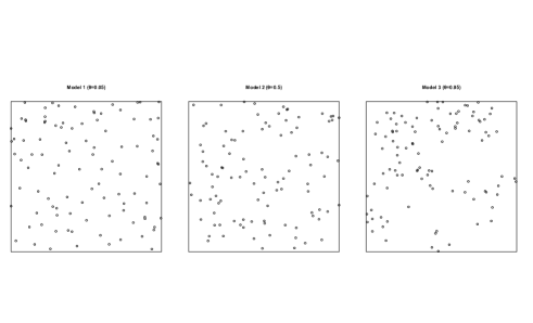
Figure 1. Simulated realizations of the three models: Model 1 (left), Model 2 (middle) and Model 3 (right).

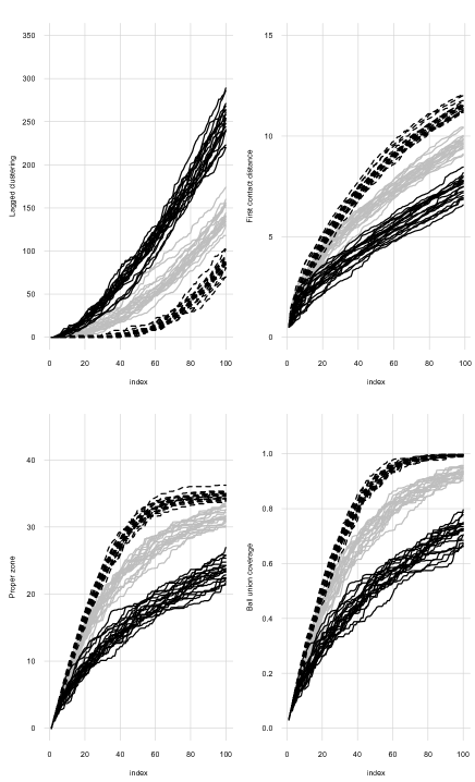
Figure 2. Summary statistics of simulated patterns of three different SSPP models. Cumulative lagged clustering statistic (top left), cumulative first contact distance (top right), cumulative proper zone statistic (bottom left), and the cumulative ball union coverage (bottom right). Dark solid lines are statistics of the Model 3, dashed lines represent those of Model 1, and grey lines are the statistics of the Model 2.

5. Application

To demonstrate the performance of the SSPP model constructed in Section 2, we need to apply it to forest stand data. Our data was collected from Kiihtelysvaara site situated in Northern Carelia, Eastern Finland (more details on stand data can be found in Packalen et al., 2013). The dataset includes 79 forest plots, however, in order to illustrate the machinery of the model, we work with two sample plots exhibiting two different spatial structures, namely Plot I and Plot II. A summary of estimated parameters of the model for all the 79 plots is given in Appendix. Dataset consists of tree locations and stem diameters measured at breast height. The Plot I contains 120 trees with minimum and maximum DBH of 4.10 cm and 23.15 cm having the mean value of 11.39 cm. In Plot II, there are 118 trees with DBH ranging from 2.30 cm as a minimum value to 41.95 cm as a maximum value, and with the mean of 12.11 cm. Figure 3 (first row) shows the patterns describing the spatial structure in Plot I and Plot II in bounded windows of sizes $25\times 25\,\textrm{m}^{2}$. In our analysis, we ignore any edge effects and all the variation of the model shall be restricted to the bounded window.

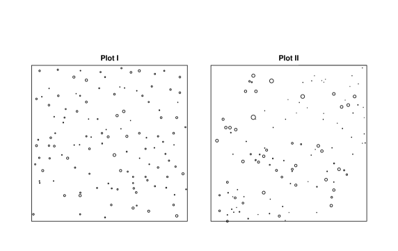
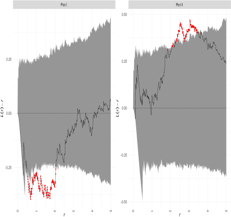
Figure 3. First row: Positions of $120$ trees (Plot I) and of $118$ trees (Plot II) in a $25\times 25$ meters sampling region in Kiihtelysvaara (Eastern Finland), where the radius of a disc is $2\times$DBH. Second row: Global envelope test for the summary $L(r)-r$ for Plot I (left) and Plot II (right) based on 4999 simulation of CSR. The grey areas show the 95% global envelopes on the interval [0,5]. The solid black line is the data function and the dashed line represents the (estimated) theoretical expectation.

A preliminary stage of the study would be an exploratory analysis using the second-order structures of the static point patterns presented in Figure 3 (first row). At this point, we adopt the linearized version of Ripley’s K-function (Ripley, , 1977; Lotwick and Silverman, , 1982) which is based on the $\mathrm{K}$-function via the formula $\mathrm{L}(r)=\sqrt{\mathrm{K}(r)/\pi}$, where $r$ is a distance between a pair of points. More details on $\mathrm{L}$-function can be found in Illian et al., (2008). Taking the centered form $\mathrm{L}(r)-r$ of the $\mathrm{L}$-function at a corresponding scale, the complete spatial randomness (CSR) is characterized by $\mathrm{L}(r)-r=0$, while values of $\mathrm{L}(r)-r$ larger than $0$ indicate clustering; the case where $\mathrm{L}(r)-r<0$ expresses regularity.

To test the complete spatial randomness hypothesis, a global envelope testing is carried out using the extreme rank length (ERL) ordering (Myllymäki et al., , 2017; Mrkvic̆ka et al., , 2018). The test is conducted using 4999 simulations of CSR on chosen interval [0,5] (in meters) for $r$, and the evaluation is represented graphically in Figure 3 (second row) indicating a rejection of the CSR hypothesis for both of the plots. The corresponding p-values of the tests are reported as $p<0.001$ and $p=0.014$ for Plot I and Plot II respectively. Apparently, the centered $\mathrm{L}$-function estimated from Plot I had negative values for distances 0.53-2.05 m below the lower envelope, which means that spatial structure of Plot I is regular at that scale. In contrast, the estimated centered $\mathrm{L}$-function of Plot II shows a clustering character at scale 1.80-3.66 m.

From the observed locations of trees in each plot, we form an ordered sequence $\overrightarrow{\mathbf{x}}_{n}=(x_{1},\ldots,x_{n})$ of these locations in a decreasing order based on DBH, where $x_{1}$ is the location of the largest tree and $x_{n}$ the location of the smallest tree in the plot.

To estimate the model parameters $\theta$ and $r$ we need to set up the ranges of these parameters. For specificity, the range of $\theta$ is obviously the interval $(0,1)$, while for the parameter $r$ we take $(\underline{r},\overline{r})$ to be the range of competition strength $(0,5)$. However, values of $r$ near the origin zero may be problematic because the stems cannot overlap. Therefore, since we lack information on ground measurements and biological knowledge, we take $\underline{r}$ to be the radius of the largest tree in the plot, so we write $\underline{r}=0.11575$ meters for Plot I and $\underline{r}=0.20975$ meters for Plot II.

Computing the integral in (3.2) requires numerical integration tools, hence, we used the Riemann sums method. To find the maximum likelihood estimate, the function is maximized over a grid of values of $(\theta,r)$ with steps $0.05$ and $0.1$ for $\theta$ and $r$ respectively. In addition, we rechecked the results by using the optimization routines implemented in the R package nloptr (Johnson, , 2010). Firstly, we employ the deterministic-search algorithm Direct-L (see Gablonsky and Kelley, , 2001) to obtain the global optimum and secondly we adjust it for greater accuracy using the Nelder-Mead simplex algorithm (Richardson and Kuester, , 1973). The maximum likelihood estimates for the Plot I and Plot II are summarized in Table 1, together with the 95% bootstrap confidence intervals calculated from 20 realizations of the fitted model (see Efron and Tibshirani, , 1994).

Table 1. Parameter estimates of SSPP model for Plot I and Plot II. The first and third columns contain MLEs obtained for the data. The second and fourth columns contain confidence intervals for the estimated parameters based on 95% bootstrap confidence intervals.

	$\hat{\theta}$	$95$% CI for $\hat{\theta}$	$\hat{r}$	$95$% CI for $\hat{r}$
Plot I	0.17	(0.13, 0.20)	2.18	(2.11, 2.25)
Plot II	0.65	(0.58, 0.74)	2.60	(1.06, 4.13)

Next we evaluate the SSPP model by computing the four summary statistics, mentioned earlier in Section 3.2, from the data and from 999 simulated realizations of the fitted model. When simulating the model, we use the observed values of the first two locations as starting points of the simulated sequence in order to reduce the unexpected variations of the simulated realizations.

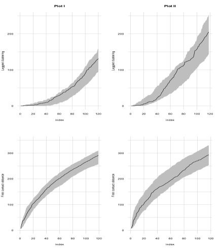
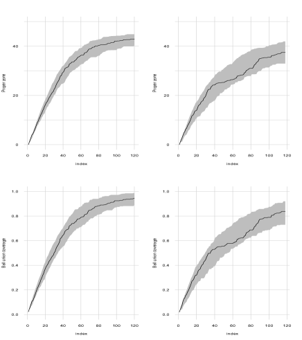
Figure 4. Summary statistics for Plot I (left column) and Plot II (right column). Cumulative lagged clustering (first row), cumulative first contact distance (second row), cumulative proper zone statistic (third row) and the cumulative ball union coverage (last row). The black solid line stands for the data, and the grey area represents pointwise envelopes estimated from 999 simulations of fitted model with parameters $(\hat{\theta},\hat{r})=(0.17,2.18)$ and $(\hat{\theta},\hat{r})=(0.65,2.60)$ for Plot I and Plot II respectively.

As can be seen in Figure 4, the four summary statistics estimated from the data stay within the simulated pointwise envelopes, which indicates that the developed SSPP model fits well showing an agreement between the data and the fitted model. Also, we were able to catch the main spatial features of interest in the forest dataset through the proposed summary statistics. On the other hand, the parameter estimates $\hat{\theta}$ and $\hat{r}$ are consistent with the exploratory study conducted by the $\mathrm{L}$-function. For the Plot I, the obtained value of $\hat{\theta}$ is small while it is large for Plot II. This indicates that the SSPP model reads the Plot I as a pattern where the new trees are choosing non-occupied locations by the previous ones in a distance greater than 2.18, which exhibits a spatial inhibition character of the pattern. For Plot II, the new points favor the locations nearby the past locations occupied by the process with a high probability value of 0.65 and within a distance of 2.60, which is explained as a cause of spatial clustering.

By writing the self-interaction term $\bm{\pi}(y,\mathbf{\mathcal{S}}_{r}(\overrightarrow{\mathbf{x}}_{k},y))=\bm{\pi}(r)$ as a function of the radius $r$ for both of the plots, we get the piecewise constant function for Plot I as:

$$\bm{\pi}(r)=\begin{cases}0&\text{if $r<0.2315$,}\\ 0.17&\text{if $0.2315\leqslant r<2.18$,}\\ 0.83&\text{if $2.18\leqslant r,$}\end{cases}$$

and for Plot II as

$$\bm{\pi}(r)=\begin{cases}0&\text{if $r<0.4195$,}\\ 0.65&\text{if $0.4195\leqslant r<2.60$,}\\ 0.35&\text{if $2.60\leqslant r.$}\end{cases}$$

The self-interaction behavior in the SSPP model can be extracted from the monotonicity of the cumulative lagged clustering function for both plots shown by the dark solid line (Figure 4). In Plot II, the cumulative lagged clustering function is growing faster to higher values than in Plot I, especially for the middle-sized trees (indexed from 40 to 80) where the cumulative ball union coverage area function also indicates a slowing behavior meaning that there is no extension of the forest area inside $W$, so these trees choose locations in the neighborhood of the bigger trees. This was different for the small-sized trees that actually look for non-occupied zones inside the window of observation, as shown by the cumulative ball union coverage area function. Also, the total coverage explains the regular and the clustered nature of Plot I and Plot II, respectively, where it approaches the total area by trees in Plot I where smaller trees choose locations nearby older ones, while trees in Plot II cover only 80% of the this total area.

On the other hand, the first contact distance function for Plot I shows a steady variation among all trees except for the first 20 trees where they avoid each others. In Plot II this statistic points out the behavior of the middle-sized trees where their first contact distances are shorter compared to other trees. The cumulative proper zone statistic did not show much variability in terms of simulations, however, trees in Plot I are sharing resources at regular pace, even when the coverage area is not extended that much anymore after the time (order) 100. This was different in Plot II where the statistic shows a slight increase of the competition by middle-sized trees.

Comparing the model interpretation with the observed data in Figure 3, we conclude that the developed SSPP model performs well by reading the self-interaction between the trees in the future and the past in both the clustered and the regular pattern, and this self-interaction property, that contains the memory and the learning through history, is well preserved under the SSPP model without loss of information.

6. Conclusion

The sequential spatial point process introduced in this paper is a special case of the class of spatio-temporal point processes where we work with ordered spatial points. In particular, this marginal process represents a bridge between the spatio-temporal point processes and the purely spatial point processes when a given order is adopted.

Our goal was to show that the mechanism of the sequential model represents a powerful modeling tool since it offers a causal description through successive conditioning, and revealing the information contained in the spatial memory. Moreover, self-interaction structure of the model enables interpreting the model parameters in terms of future-past dependence in a dynamic form. An additional advantage of the model is that it is likelihood-based allowing to use well-defined statistical tools in analyzing data. However, evaluating the model requires constructing summary statistics that better describe the features of the phenomena in terms of order, which are seldom considered in the literature. For this, we used real data and we utilized four summary statistics to evaluate the potential variations of data assisted by Monte Carlo simulation. Since the functions are in terms of time/order, they allow us to catch the variation of the feature in question. In our application, we were able to distinguish between the variation exhibited by each class of tree sizes, large, medium-sized, and small.

Although the SSPP model was able to read patterns with different aggregations, the concept of the sequential model presented in this paper differs from other spatial point processes in the sense that it is interpreting the structure of observed patterns beyond the general regular-clustered definition. It is reading their aggregation at a certain specific range given by the parameter $r$. In contrast one could fix this parameter in an approach similar to Penttinen and Ylitalo, (2016), or more generally, propose a collection of suitable $r$ values representing the range of competition strength. This has an advantage in laser scanning application where the fixed $r$ could represent the crown radius of the tree, therefore the only parameter to be estimated would be $\theta$.

The order of the spatial dimension given in the paper emphasizes the dynamic evolution of the forest stand, as we believe that the trees with larger sizes appear earlier than the small ones. Hence, our objective was to switch from the static point patterns to a dynamic one where the information that lies within the elevated spatial history is of great importance. However, other orders can be used when applying the sequential spatial point processes which might depend on the context and on the observed phenomena.

It is clear that our model depends on the order used for the spatial points, i.e., when choosing different order, the interactions between a point and its past will definitely influence the density and the probabilistic properties of the process, except for the case of $\theta=0.5$ where the density is invariant under the choice of the order. This immediately reflects the non-exchangeability property of the model which usually does not exist in most of the structures of spatial point processes. The analysis introduced in this paper can be extended to compare different types of ordering for static point patterns, which is a future task.

Appendix

The following tables are referenced in Section 5. Tables contain summary of the estimated parameters of the 79 plots, associated with plots metrics.

Table 2. First column indicates the plot identification number from 79 forest plots in Kiihtelysvaara. Columns 2-5 calculate the estimated parameters $\hat{\theta}$ and $\hat{r}$ and their associated bootstrap 95% confidence intervals. Columns 6-10 contain characteristics of the plot as follows: The number of trees in the plot, the minimum, the maximum and the mean values of the diameters measured at breast height (DBH) of trees in the plot (cm). Last column shows the size of the plot (m). Plot I and Plot II considered in the study are the plots with identification number 5 and 74 respectively

Plot id.	$\hat{\theta}$	$95$% CI for $\hat{\theta}$	$\hat{r}$	$95$% CI for $\hat{r}$	Nb. of indiv.	Min. DBH (cm)	Max. DBH (cm)	Mean DBH (cm)	Plot size (m $\times$ m)
$1$	$0.20$	(0.11, 0.28)	$3.80$	(3.69, 3.90)	$114$	$3.00$	$44.50$	$15.31$	30 x 30
$2$	$0.30$	(0.25, 0.35)	$3.25$	(3.07, 3.43)	$73$	$3.05$	$34.00$	$14.28$	25 x 25
$3$	$0.23$	(0.17, 0.28)	$2.42$	(2.23, 2.60)	$54$	$4.25$	$29.00$	$17.48$	25 x 25
$4$	$0.39$	(0.27, 0.50)	$3.13$	(2.11, 4.14)	$100$	$3.90$	$26.30$	$12.31$	25 x 25
$5$	$0.17$	(0.13, 0.19)	$2.18$	(2.12, 2.25)	$120$	$4.10$	$23.15$	$11.39$	25 x 25
$6$	$0.34$	(0.31, 0.37)	$3.15$	(2.57, 3.74)	$104$	$4.20$	$50.10$	$17.64$	30 x 30
$7$	$0.75$	(0.69, 0.81)	$0.50$	(0.35, 0.65)	$104$	$3.45$	$36.75$	$13.53$	30 x 30
$8$	$0.11$	(0.06, 0.16)	$1.20$	(1.13, 1.27)	$59$	$2.50$	$32.20$	$17.62$	24 x 25
$9$	$0.21$	(0.17, 0.25)	$1.39$	(0.44, 2.32)	$133$	$3.85$	$27.40$	$13.91$	25 x 25
$10$	$0.14$	(0.13, 0.15)	$1.49$	(1.24, 1.74)	$125$	$3.95$	$28.10$	$13.78$	25 x 25
$11$	$0.83$	(0.75, 0.91)	$7.96$	(7.28, 8.64)	$48$	$3.30$	$36.80$	$17.20$	25 x 25
$12$	$0.37$	(0.30, 0.44)	$1.31$	(0.95, 1.68)	$160$	$2.30$	$21.60$	$9.25$	24 x 25
$13$	$0.30$	(0.17, 0.43)	$3.45$	(2.55, 4.35)	$48$	$4.95$	$37.35$	$17.38$	25 x 25
$14$	$0.16$	(0.13, 0.19)	$4.25$	(4.15, 4.35)	$34$	$4.05$	$39.60$	$21.06$	25 x 25
$15$	$0.14$	(0.10, 0.17)	$1.19$	(1.15, 1.22)	$89$	$3.05$	$18.25$	$11.50$	20 x 20
$16$	$0.18$	(0.14, 0.22)	$1.42$	(1.28, 1.55)	$89$	$3.45$	$27.85$	$13.49$	25 x 25
$17$	$0.23$	(0.18, 0.28)	$1.79$	(1.61, 1.97)	$61$	$3.20$	$22.20$	$10.53$	20 x 20
$18$	$0.09$	(0.07, 0.11)	$1.49$	(1.45, 1.53)	$77$	$2.30$	$21.95$	$13.55$	20 x 20
$19$	$0.88$	(0.84, 0.93)	$6.78$	(6.19, 7,38)	$68$	$5.15$	$36.55$	$16.86$	25 x 25
$20$	$0.11$	(0.07, 0.15)	$0.92$	(0.85, 0.98)	$81$	$2.50$	$23.40$	$13.63$	20 x 20
$21$	$0.80$	(0.75, 0.85)	$0.40$	(0.24, 0.55)	$101$	$2.85$	$25.70$	$10.83$	25 x 25
$22$	$0.13$	(0.10, 0.16)	$1.32$	(1.19, 1.45)	$82$	$2.95$	$24.50$	$14.49$	25 x 25
$23$	$0.20$	(0.13, 0.27)	$3.50$	(2.76, 4.23)	$65$	$2.10$	$28.15$	$13.49$	20 x 20
$24$	$0.35$	(0.22, 0.48)	$1.19$	(0.48, 1.90)	$65$	$4.25$	$25.05$	$12.72$	25 x 25
$25$	$0.61$	(0.56, 0.66)	$0.86$	(0.63, 1.09)	$82$	$2.65$	$28.20$	$10.61$	20 x 20
$26$	$0.95$	(0.83, 1.06)	$0.15$	(0.03, 0.27)	$72$	$3.35$	$24.20$	$12.84$	25 x 25
$27$	$0.23$	(0.19, 0.26)	$2.61$	(2.51, 2.70)	$45$	$3.00$	$21.90$	$15.03$	25 x 25
$28$	$0.39$	(0.36, 0.42)	$1.91$	(1.58, 2.24)	$58$	$2.45$	$22.65$	$9.75$	20 x 20
$29$	$0.80$	(0.75, 0.85)	$0.55$	(0.26, 0.84)	$58$	$3.00$	$48.75$	$12.40$	20 x 20
$30$	$0.20$	(0.14, 0.25)	$1.75$	(1.63, 1.87)	$47$	$4.15$	$29.00$	$17.52$	25 x 25

Table 3. Contined.

Plot id.	$\hat{\theta}$	$95$% CI for $\hat{\theta}$	$\hat{r}$	$95$% CI for $\hat{r}$	Nb. of indiv.	Min. DBH (cm)	Max. DBH (cm)	Mean DBH (cm)	Plot size (m $\times$ m)
$31$	$0.12$	(0.06, 0.17)	$1.77$	(1.74, 1.80)	$51$	$2.20$	$25.55$	$17.40$	25 x 25
$32$	$0.25$	(0.15, 0.34)	$3.90$	(3.08, 4.72)	$64$	$3.10$	$24.95$	$13.97$	25 x 25
$33$	$0.95$	(0.91, 0.99)	$6.55$	(5.90, 7.20)	$85$	$2.20$	$28.75$	$10.39$	20 x 20
$34$	$0.33$	(0.31, 0.35)	$2.32$	(1.92, 2.72)	$84$	$1.95$	$30.75$	$13.48$	25 x 25
$35$	$0.73$	(0.69, 0.76)	$2.15$	(1.99, 2.31)	$71$	$1.90$	$23.80$	$10.53$	20 x 20
$36$	$0.24$	(0.12, 0.36)	$4.90$	(3.46, 6.35)	$57$	$2.30$	$31.50$	$14.26$	20 x 20
$37$	$0.35$	(0.24, 0.46)	$1.01$	(0.24, 1.78)	$50$	$2.60$	$33.25$	$16.32$	25 x 25
$38$	$0.25$	(0.18, 0.31)	$2.89$	(2.51, 3.27)	$39$	$2.65$	$31.05$	$17.49$	25 x 25
$39$	$0.13$	(0.11, 0.15)	$4.00$	(3.89, 4.12)	$75$	$1.90$	$37.70$	$8.78$	19 x 20
$40$	$0.13$	(0.09, 0.17)	$3.23$	(3.16, 3.30)	$32$	$13.10$	$33.95$	$21.84$	25 x 25
$41$	$0.20$	(0.14, 0.26)	$2.90$	(2.81, 2.99)	$38$	$3.20$	$25.55$	$15.37$	25 x 25
$42$	$0.39$	(0.29, 0.48)	$0.87$	(0.19, 1.56)	$72$	$5.15$	$23.70$	$14.25$	20 x 20
$43$	$0.24$	(0.21, 0.27)	$1.32$	(1.17, 1.48)	$90$	$2.20$	$21.50$	$12.85$	20 x 20
$44$	$0.17$	(0.13, 0.21)	$0.99$	(0.87, 1.11)	$85$	$2.50$	$24.35$	$11.47$	20 x 20
$45$	$0.19$	(0.15, 0.23)	$2.20$	(1.59, 2.82)	$51$	$3.95$	$22.50$	$15.85$	25 x 25
$46$	$0.13$	(0.07, 0.20)	$1.41$	(1.32, 1.50)	$64$	$3.00$	$22.35$	$13.73$	25 x 25
$47$	$0.30$	(0.24, 0.36)	$0.95$	(0.60, 1.29)	$81$	$1.90$	$23.25$	$10.06$	20 x 20
$48$	$0.26$	(0.23, 0.30)	$2.82$	(2.51, 3.13)	$64$	$2.05$	$26.10$	$15.43$	25 x 25
$49$	$0.17$	(0.13, 0.20)	$4.40$	(4.24, 4.55)	$52$	$2.45$	$28.40$	$12.40$	25 x 25
$50$	$0.62$	(0.59, 0.66)	$1.27$	(0.97, 1.58)	$113$	$2.95$	$44.05$	$15.66$	30 x 30
$51$	$0.12$	(0.10, 0.15)	$2.69$	(2.60, 2.77)	$42$	$5.90$	$40.80$	$28.40$	30 x 30
$52$	$0.12$	(0.08, 0.16)	$2.00$	(1.18, 2.17)	$51$	$5.05$	$38.65$	$25.78$	30 x 30
$53$	$0.14$	(0.11, 0.16)	$2.49$	(2.42, 2.56)	$49$	$2.15$	$40.75$	$26.44$	30 x 30
$54$	$0.09$	(0.06, 0.13)	$2.23$	(2.16, 2.31)	$40$	$4.30$	$37.80$	$18.50$	25 x 25
$55$	$0.14$	(0.11, 0.16)	$3.60$	(3.47, 3.72)	$46$	$3.20$	$34.80$	$18.37$	25 x 25
$56$	$0.21$	(0.15, 0.28)	$1.47$	(1.31, 1.63)	$70$	$2.40$	$48.65$	$17.36$	30 x 30
$57$	$0.33$	(0.30, 0.36)	$3.05$	(2.61, 3.50)	$58$	$2.10$	$32.80$	$18.65$	30 x 30
$58$	$0.06$	(0.03, 0.08)	$1.87$	(1.82, 1.92)	$45$	$2.35$	$26.95$	$17.82$	25 x 25
$59$	$0.21$	(0.18, 0.24)	$2.83$	(2.32, 3.33)	$54$	$2.00$	$35.10$	$13.59$	25 x 25
$60$	$0.21$	(0.19, 0.23)	$2.21$	(1.81, 2.61)	$50$	$4.40$	$43.00$	$17.60$	25 x 25

Table 4. Continued

Plot id.	$\hat{\theta}$	$95$% CI for $\hat{\theta}$	$\hat{r}$	$95$% CI for $\hat{r}$	Nb. of indiv.	Min. DBH (cm)	Max. DBH (cm)	Mean DBH (cm)	Plot size (m $\times$ m)
$61$	$0.33$	(0.30, 0.36)	$3.15$	(2.54, 3.76)	$56$	$3.60$	$36.65$	$17.29$	30 x 30
$62$	$0.28$	(0.25, 0.32)	$2.23$	(2.00, 2.46)	$79$	$3.40$	$31.75$	$16.62$	30 x 30
$63$	$0.21$	(0.18, 0.23)	$3.00$	(2.86, 3.15)	$59$	$4.35$	$37.20$	$19.72$	30 x 30
$64$	$0.25$	(0.19, 0.31)	$3.55$	(3.31, 3.78)	$81$	$3.75$	$40.00$	$12.38$	25 x 25
$65$	$0.22$	(0.20, 0.25)	$1.80$	(1.70, 1.90)	$101$	$3.35$	$40.45$	$14.67$	25 x 25
$66$	$0.22$	(0.20.0.25)	$2.11$	(1.75, 2.48)	$64$	$3.35$	$33.65$	$18.41$	30 x 30
$67$	$0.25$	(0.21, 0.29)	$2.45$	(2.24, 2.66)	$57$	$4.85$	$34.10$	$20.88$	30 x 30
$68$	$0.17$	(0.14, 0.20)	$2.00$	(1.59, 2.41)	$60$	$2.30$	$31.70$	$18.36$	25 x 25
$69$	$0.28$	(0.21, 0.34)	$2.19$	(1.61, 2.77)	$49$	$3.75$	$36.25$	$21.97$	30 x 30
$70$	$0.35$	(0.30, 0.40)	$1.08$	(0.69, 1.46)	$85$	$4.05$	$30.65$	$12.08$	20 x 20
$71$	$0.33$	(0.23, 0.43)	$3.90$	(2.98, 4.82)	$115$	$4.25$	$26.70$	$10.78$	20 x 20
$72$	$0.11$	(0.08, 0.15)	$2.05$	(1.96, 2.15)	$33$	$4.90$	$27.55$	$19.05$	20 x 20
$73$	$0.31$	(0.18, 0.43)	$2.50$	(1.72, 3.27)	$55$	$3.35$	$27.10$	$12.87$	20 x 20
$74$	$0.65$	(0.58, 0.74)	$2.60$	(1.06, 4.13)	$118$	$2.30$	$41.95$	$12.11$	30 x 30
$75$	$0.33$	(0.26, 0.41)	$3.90$	(3.02, 4.78)	$113$	$1.60$	$39.40$	$8.14$	25 x 25
$76$	$0.65$	(0.60, 0.70)	$1.20$	(0.87, 1.53)	$105$	$2.65$	$28.75$	$14.13$	25 x 25
$77$	$0.22$	(0.19, 0.26)	$5.87$	(5.77, 5.96)	$84$	$2.85$	$49.10$	$13.38$	25 x 25
$78$	$0.80$	(0.77, 0.83)	$0.50$	(0.44, 0.56)	$100$	$2.70$	$39.15$	$9.37$	25 x 25
$79$	$0.30$	(0.26, 0.33)	$1.00$	(0.82, 1.18)	$94$	$3.20$	$19.45$	$10.95$	25 x 25

References

- Baddeley et al., (2015) Baddeley, A., Rubak, E., and Turner, R. (2015). Spatial Point Patterns: Methodology and Applications with R. Chapman & Hall/CRC.
- Cressie, (1993) Cressie, N. A. C. (1993). Statistics for Spatial Data. Wiley.
- Daley and Vere-Jones, (2003) Daley, D. J. and Vere-Jones, D. (2003). An Introduction to the Theory of Point Processes. Volume I: Elementary Theory and Methods. New York: Springer-Verlag.
- Daley and Vere-Jones, (2008) Daley, D. J. and Vere-Jones, D. (2008). An Introduction to the Theory of Point Processes. Volume II: General Theory and Structure. New York: Springer-Verlag.
- Davison, (2008) Davison, A. C. (2008). Statistical Models. Cambridge University Press.
- Diggle, (2013) Diggle, P. J. (2013). Statistical Analysis of Spatial and Spatio-Temporal Point Patterns. Chapman & Hall/CRC.
- Diggle et al., (1976) Diggle, P. J., Besag, J., and Gleaves, J. T. (1976). Statistical analysis of spatial point patterns by means of distance methods. Biometrics, pages 65–667.
- Efron and Tibshirani, (1994) Efron, B. and Tibshirani, R. J. (1994). An Introduction to the Bootstrap. Chapman and Hall/CRC Press.
- Evans, (1993) Evans, J. V. (1993). Random and cooperative sequential adsorption. Reviews of Modern Physics, 65:1281–1330.
- Gablonsky and Kelley, (2001) Gablonsky, J. and Kelley, C. (2001). A locally-biased form of the direct algorithm. Journal of Global Optimization, 21:27–37.
- González et al., (2016) González, J. A., Rodríguez-Cortés, F. J., Cronie, O., and Mateu, J. (2016). Spatio-temporal point process statistics: A review. Spatial Statistics, 18:505–544.
- Illian et al., (2008) Illian, J., Penttinen, A., Stoyan, H., and Stoyan, D. (2008). Statistical Analysis and Modeling of Spatial Point Patterns. Wiley, Chichester, UK.
- Jensen et al., (2007) Jensen, E. B. V., Jónsdóttir, K. Y., Schmiegel, J., and Barndorff-Nielsen, O. E. (2007). Spatio-temporal modelling with a view to biological growth. Statistical methods for spatio-temporal systems, Monographs on statistics and applied probability, pages 47–75.
- Johnson, (2010) Johnson, S. G. (2010). The nlopt nonlinear-optimization package. http://ab-initio.mit.edu/nlopt.
- Kansanen et al., (2016) Kansanen, K., Vauhkonen, J., Lähivaara, T., and Mehtätalo, L. (2016). Stand density estimators based on individual tree detection and stochastic geometry. Canadian Journal of Forest Research, 46:1359–1366.
- (16) Lieshout, M. (2006a). Campbell and moment measures for finite sequential spatial processes. Proceedings Prague Stochastics, 48:215–224.
- (17) Lieshout, M. (2006b). Markovianity in space and time. IMS Lecture Notes–Monograph Series, 48:154–168.
- (18) Lieshout, M. (2006c). Maximum likelihood estimation for random sequential adsorption. Advances in Applied Probability (SGSA), 38:889–898.
- Lieshout and Capasso, (2009) Lieshout, M. and Capasso, V. (2009). Sequential spatial processes for image analysis. Electronic Transactions on Numerical Analysis.
- Lotwick and Silverman, (1982) Lotwick, H. W. and Silverman, B. W. (1982). Methods for analyzing spatial processes of several types of points. J. Roy. Stat. Soc. Series B, 44:406–413.
- Maltamo et al., (2014) Maltamo, M., Naesset, E., and Vauhkonen, J. (2014). Forestry Applications of Airborne Laser Scanning Concepts and Case Studies. Springer.
- Mehtätalo, (2006) Mehtätalo, L. (2006). Eliminating the effect of overlapping crowns from aerial inventory estimates. Canadian Journal of Forest Research, 36:1649–1660.
- Møller et al., (2016) Møller, J., Ghorbani, M., and Rubak, E. (2016). Mechanistic spatio-temporal point process models for marked point processes, with a view to forest stand data. Biometrics, 72:687–696.
- Møller and Waagepetersen, (2004) Møller, J. and Waagepetersen, R. P. (2004). Statistical Inference and Simulation for Spatial Point Processes. Chapman & Hall/CRC.
- Mrkvic̆ka et al., (2018) Mrkvic̆ka, T., Myllymäki, M., Jilek, M., and Hahn, U. (2018). A one-way anova test for functional data with graphical interpretation. ArXiv:1612.03608.
- Myllymäki et al., (2017) Myllymäki, M., Mrkvic̆ka, T., Grabarnik, P., Seijo, H., and Hahn, U. (2017). Global envelope tests for spatial processes. Journal of the Royal Statistical Society Series B (Statistical Methodology), 79:381–404.
- Packalen et al., (2013) Packalen, P., Vauhkonen, J., Kallio, E., Peuhkurinen, J., Pitkänen, J., Pippuri, I., Strunk, J., and Maltamo, M. (2013). Predicting the spatial pattern of trees by airborne laser scanning. International Journal of Remote Sensing, 34(14):5154–5165.
- Penttinen and Ylitalo, (2016) Penttinen, A. and Ylitalo, A. K. (2016). Deducing self-interaction in eye movement data using sequential spatial point processes. Spatial Statistics, 17:1–21.
- Richardson and Kuester, (1973) Richardson, J. A. and Kuester, J. L. (1973). The complex method for constrained optimization. Communications of the ACM, 16:487–489.
- Ripley, (1977) Ripley, B. D. (1977). Modeling spatial patterns. J. Roy. Stat. Soc. Series B, 39:172–212.
- Ripley, (1987) Ripley, B. D. (1987). Stochastic simulation. Wiley.
- Snyder and Miller, (1991) Snyder, D. L. and Miller, M. I. (1991). Random Point Processes in Time and Space. Springer.
- Stoyan et al., (2017) Stoyan, D., Rodríguez-Cortés, F. J., Mateu, J., and Gille, W. (2017). Mark variograms for spatio-temporal point processes. Spatial Statistics, 20:125–147.
- Talbot et al., (2000) Talbot, J., Tarjus, G., Van Tassel, P. R., and Viot, P. (2000). From car parking to protein adsorption: An overview of sequential adsorption processes. Colloids and Surfaces A: Physicochemical and Engineering Aspects, 165:28–324.
- Vere-Jones, (2009) Vere-Jones, D. (2009). Some models and procedures for space-time point processes. Environmental and Ecological Statistics, 16:173–195.
- Ylitalo, (2017) Ylitalo, A. K. (2017). Statistical inference for eye movement sequences using spatial and spatio-temporal point processes. PhD thesis, University of Jyväskylä, Department of Mathematics and Statistics. Report 160.