Self-Adaptive Network Pruning

Abstract

Deep convolutional neural networks have been proved successful on a wide range of tasks, yet they are still hindered by their large computation cost in many industrial scenarios. In this paper, we propose to reduce such cost for CNNs through a self-adaptive network pruning method (SANP). Our method introduces a general Saliency-and-Pruning Module (SPM) for each convolutional layer, which learns to predict saliency scores and applies pruning for each channel. Given a total computation budget, SANP adaptively determines the pruning strategy with respect to each layer and each sample, such that the average computation cost meets the budget. This design allows SANP to be more efficient in computation, as well as more robust to datasets and backbones. Extensive experiments on 2 datasets and 3 backbones show that SANP surpasses state-of-the-art methods in both classification accuracy and pruning rate.

1 Introduction

Recently, convolutional neural networks (CNNs) have become a dominant approach in a wide range of visual tasks. Typical applications of CNNs include image classification Krizhevsky et al. (2012), object detection Girshick et al. (2014) and semantic segmentation Long et al. (2015). Despite their success, it is still a challenge to deploy CNNs in industrial scenarios. This is mainly because CNNs are designed to be over-parameterized Du et al. (2019), and require much computation during inference. For example, ResNet-18, the smallest version of ResNet He et al. (2016), requires 2 GFLOPs for a single prediction, which is unaffordable for most smartphones or embedded systems.

To reduce the computation demand of CNNs, many methods have been proposed from several perspectives. A bunch of methods Chollet (2017)Zhang et al. (2018)Ma et al. (2018) propose to build efficient architectures with depthwise separable convolutions. Some methods Courbariaux et al. (2016)Zhou et al. (2016)Micikevicius et al. (2018) learn models for low-precision inference. However, these methods require careful design of models or quantization functions, which can hardly generalize to other tasks without heavy engineering. Most recently, there are a number of methods Han et al. (2016)Li et al. (2017)Liu et al. (2017) that try to prune the connections in networks. These methods drop parameters or channels according to some saliency scores, such as $L_{1}$-norm values of parameters or channels. As the scores are adaptively computed with regard to the model as well as the task, these methods can be easily applied to different scenarios. Therefore, we also follow this stream in this paper, and propose a novel self-adaptive pruning method.

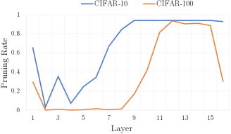
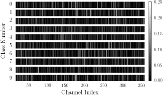
Figure 1: Visualization of channel activations in a pruned VGGNet. (a) Pruning rate w.r.t. layers. The pruning rate varies from layer to layer on both datasets. (b) Average activation of each channel in the last convolutional layer w.r.t. categories in CIFAR-100. Only a small subset of channels is activated for each category.

Typically, a network pruning recipe at channel level consists of 2 ingredients, a saliency estimation module and a pruning module. Given a budget, the pruning algorithms Li et al. (2017)Liu et al. (2017) first learn saliency scores for each channel, and then prune channels that have low scores. However, we argue this formulation is not enough for a good pruning. Take VGGNet Simonyan & Zisserman (2014) pruned by Network Slimming (NS) Liu et al. (2017) as an example, we observe two phenomena:

1. For different layers, the optimal pruning rates are very different.

2. For each category, it only activates a small subset of remaining channels.

Figure 1 illustrates these phenomena. The first phenomenon shows that there does not exist a constant pruning rate for every layer. In other words, layers would be either over-pruned or under-pruned by any global pruning rate. This is because most CNN architectures are designed for ImageNet, and the capacity of layers does not necessarily fit CIFAR-10, CIFAR-100 and other datasets. Hence, a good pruning strategy should set different pruning rates for each layer. The second phenomenon indicates that a static pruning strategy is sub-optimal, since only a small set of channels is required for each category. To get better pruning performance, the pruning strategy needs to be conditioned on the input images. Ideally, we would like to have a pruning method that has both properties.

In this paper, we propose a self-adaptive method (SANP) for network pruning. Our method satisfies the above two properties through a layer-adaptive and sample-adaptive design. Specifically, the layer adaptiveness is achieved by a cost estimation step for each layer, with only budget constraints on the total computation cost. The sample adaptiveness is achieved by a saliency prediction step over the current input sample. Both steps utilize differentiable modules and thereby can be jointly trained with classification objective using a multi-task loss. Our method adaptively determines the computation routine for each layer and each sample, and improves the pruning rate over state-of-the-art methods, without sacrifice on performance. The contribution of this paper is three folds:

1. We propose a novel method SANP for network pruning, which adaptively learns the pruning rate for each layer and each sample.

2. We instantiate SANP with differentiable modules, and enable joint training with classification and cost objectives.

3. We empirically evaluate our method on 2 datasets and 3 backbones and it achieves state-of-the-art performance in all settings.

2 Related Works

2.1 Static Network Pruning

Static pruning methods generate a fixed network for all novel images. They can be divided into weight pruning methods and channel pruning methods. Weight pruning methods work on pruning fine-grained weights of the filters, resulting in unstructured sparsity. For example, Han et al. Han et al. (2016) iteratively prune near-zero weights to obtain a pruned network without loss of precision. Channel pruning methods reduce model size at channel level and can achieve a sparse structure. Li et al. (2017) iteratively prunes filters whose $L_{1}$-norm values are relatively small and retrains the remaining network. NS Liu et al. (2017) introduces sparsity on the scaling parameters of Batch Normalization (BN) layers and proposes an iterative two-step algorithm to prune the network. AutoPruner Luo & Wu (2018) integrates channel pruning and model fine-tuning into a single end-to-end trainable framework. Filter Clustering and Pruning (FCP) Zhou et al. (2018) adds an extra cluster loss to the loss function, which forces the filters in each cluster to be similar and thereby prunes redundant channels. NS, AutoPruner and FCP could adaptively determine pruning rate for each layer, but their pruning strategies are invariant with regard to different samples.

2.2 Dynamic Path Network

Instead of using the entire feed forward graph of the network, dynamic path networks Lin et al. (2017)Liu & Deng (2018)Hua et al. (2018)Gao et al. (2019) selectively execute a subset of modules at inference time based on input samples. Runtime Neural Pruning Lin et al. (2017) uses an agent to judge channel importance and prunes unimportant channels according to different samples with reinforcement learning. Liu et al. Liu & Deng (2018) propose a dynamic deep neural network to execute a subset of neurons and use deep Q-learning to train the controller modules. The above dynamic networks train their strategies through reinforcement learning because the binary decisions cannot be represented by differentiable functions. Therefore these methods are hard to generalize on multiple datasets and networks. Recently, several methods overcome this limitation. Channel Gating (CG) Hua et al. (2018) splits channels in each layer into two groups and the proportion of the first group is uniform for all layers. Then it identifies ineffectual receptive fields based on the first group of channels and skips computation on the second group in these fields. It uses continuous functions to approximate the gradient of non-differentiable binary functions. Feature Boosting and Suppression (FBS) Gao et al. (2019) sets a constant pruning rate for each layer and amplifies salient channels based on the current input sample. It utilizes a k-winners-take-all function which is partially differentiable. Though both CG and FBS are sample-adaptive methods, they lack layer-adaptiveness to regulate pruning rate for different layers.

3 Our Method

Figure 2 shows the main pipeline of SANP. Firstly, Saliency-and-Pruning Module is embedded in each convolutional layer of backbone network. It predicts saliency scores for channels based on input features and then generates pruning decision for each channel. The convolution operation would be skipped for these channels whose corresponding pruning decision is 0, as indicated by the dashed arrow. Then we jointly train the backbone network and SPMs with both classification objective and cost objective. We estimate computation cost dependent on the pruning decisions in each layer. The estimation adjusts importance of two objectives so that network could adaptively determine pruning rate per layer with a total computation budget. Since input features and output features are both sparse, the expensive convolution operation can be accelerated from both sides. Then we will go into details about the proposed method.

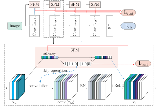
Figure 2: The overall pipeline and layer pipeline of SANP. Colors of channels indicate their saliency scores, where white denotes zero saliency. First, the input features are down-sampled and passed into SPM to get saliency scores and pruning decisions for channels. Then channel pruning decisions are used to estimate current computation cost. The estimation automatically adjusts importance of classification loss and cost loss so that the network adaptively determines pruning rate for each layer with regard to the computation budget.

3.1 Saliency-and-Pruning Module

To prune channels layer-by-layer, some modules or separate networks are required. And the pruning strategy must be decided before each layer is activated. We propose a Saliency-and-Pruning Module, a lightweight network module for this purpose.

Since we observe that only a subset of channels is actually activated for different categories, we decide to determine channel pruning strategy dependent on each input image to get better performance. And in order to adaptively find the most important channels for each sample, we generate saliency scores for kernels based on the input features from previous layer $x^{l-1}\in\mathbb{R}^{C_{l-1}\times H_{l-1}\times W_{l-1}}$. Saliency prediction can be defined as

$$s^{l}(x^{l-1})=SaliencyPrediction(x^{l-1},W)$$ (1)

where $SaliencyPrediction(\cdot)$ denotes saliency function. In Section 3.2, we would introduce this function specifically.

Then the channels with low saliency scores could be pruned so as to accelerate backbone network. We need to adopt 0/1 binary valued function to decide whether the calculation of each channel is skipped or not. However, binary functions are not differentiable and thereby these problems are usually approached with reinforcement learning. Unlike previous work, we utilize a discretization technique called Improved Semantic Hashing Kaiser & Bengio (2018), which enables classification loss back-propagate to SPMs. Hence, the backbone network and SPMs could be jointly trained in an end-to-end manner. The pruning decisions could be formulated as:

$$b^{l}(x^{l-1})=Binarize(s^{l-1})$$ (2)

where $Binarize(\cdot$) denotes binarization function.In Section 3.3, we would introduce this function specifically.

Further, channels with higher saliency scores are naturally the more significant channels, therefore we propose to rescale the output features with saliency scores to make these channels more decisive. Since modern deep neural networks He et al. (2016)Huang et al. (2017)Zhang et al. (2018) apply BN layers after convolutional layers, we leverage the rescaling operation directly after each BN layer. Here, we propose to define the calculation of a batch-normalized convolutional layer with SPM. The $i^{th}$ channel of output features $x^{l}\in\mathbb{R}^{C_{l}\times H_{l}\times W_{l}}$ is formulated as:

$$x_{i}^{l}=s_{i}^{l}(x^{l-1})\cdot b_{i}^{l}(x^{l-1})\cdot BatchNorm(f_{i}^{l}\ast x^{l-1})$$ (3)

where $f_{i}^{l}$ denotes the $i^{th}$ convolutional kernel of $l^{th}$ layer and $\ast$ denotes convolution operation. Since $b^{l}$ is a binary code, we can reformulate the computation of $x_{i}^{l}$:

$$x_{i}^{l}=\left\{\begin{array}[]{lr}\textbf{0},&if\ \ b_{i}^{l}=0\\ s_{i}^{l}(x^{l-1})\cdot b_{i}^{l}(x^{l-1})\cdot BatchNorm(f_{i}^{l}\ast x^{l-1}),&if\ \ b_{i}^{l}\neq 0\end{array}\right.$$ (4)

Here 0 is a 2-D feature map with all its elements being 0. That is, if $b_{i}^{l}$=0, convolution operation of filter $f_{i}^{l}$ is skipped and 0 is used as the output instead. All convolutions can take advantage of both input-side and output-side sparsity. Additionally, $C_{l}$ denotes the channel number of $x^{l}$, $H_{l}$ and $W_{l}$ denotes the height and width of feature map.

3.2 Saliency Function

To obtain saliency, we firstly use global average pooling to squeeze global spatial information into a channel descriptor following SEblock Hu et al. (2018). Specifically, the channel descriptor $d\in\mathbb{R}^{C_{l-1}}$ is calculated by the following formula:

$$d=\frac{1}{H_{l-1}\times W_{l-1}}\sum_{i=1}^{H_{l-1}}\sum_{j=1}^{W_{l-1}}x^{l-1}(i,j)$$ (5)

Then we consider using fully-connected layers to map channel-wise statics to predict saliency scores for kernels in $l^{th}$ layer. In order to reduce computation, we use a reduction rate r like SEblockHu et al. (2018). The saliency scores $s\in\mathbb{R}^{C_{l}}$ can be defined as:

$$s^{l}(x^{l-1})=SaliencyPrediction(x^{l-1},W)=W_{2}\delta(W_{1}d)$$ (6)

where $\delta$ refers to the ReLU function, $W_{1}\in\mathbb{R}^{\frac{C_{l}}{r}\times C_{l-1}}$, $W_{2}\in\mathbb{R}^{C_{l}\times\frac{C_{l}}{r}}$.

3.3 Binarization Function

We adopt a recently proposed discretization technique namely Improved Semantic Hashing Kaiser & Bengio (2018) to generate channel pruning strategy from saliency scores $s^{l}$($x^{l-1}$).

During training, a Gaussian noise $\xi\sim N(0,1)^{C_{l}}$ is add to $s^{l}(x^{l-1})$. As with all of the operations below, the sum operation is element-wise. Then we compute the vector through a saturating sigmoid function Kaiser & Sutskever (2015):

$$s_{1}=\max(0,\min(1,a\cdot\sigma(s^{l}(x^{l-1})+\xi)-b))$$ (7)

where $\sigma$ denotes the original sigmoid function, $a$ and $b$ denote hyperparameters.

The binary code is then constructed via rounding:

$$s_{2}=\mathbbm{1}(s_{1}>0.5)$$ (8)

In the forward propagation, we use $s_{1}$ half of the time and $s_{2}$ the other half. $s_{2}$ is computed from non-differentiable function. Therefore in the backward propagation, we let gradients always flow to $s_{1}$, even if $s_{2}$ is used in the forward propagation.

During evaluation and inference, $s_{2}$ is used all the time. Note that the Gaussian noise is only used for training and we set $\xi$ to 0 during evaluation and inference.

3.4 Multi-task Training

Until now, one question remains that how to control sparsity of the network, so that it reaches a computation budget. We observe that the optimal pruning rate varies with different layers and thereby the pruning method should adaptively learn pruning rate for each layer. To solve this problem, we propose a multi-task training with both classification objective and cost objective. We induce network sparsity with $L_{1}$-norm on saliency scores and estimate the current computation cost with pruning decisions generated by SPMs in each layer. The cost estimation adjusts importance of two objectives so that network could adaptively determine pruning rate for each layer with a total computation budget. The multi-task loss could be formulated as:

$$\mathcal{L}_{multi}=\mathcal{L}_{cls}+\lambda\frac{1}{N_{c}}\sum_{l=1}^{L}\|s^{l}\|_{1}$$ (9)

where the first term is a classification loss (e.g., cross entropy loss), and the second term is the cost loss $\mathcal{L}_{cost}$. $N_{c}$ denotes total filter number of backbone network, $L$ denotes total layers of backbone network.

The value of $\lambda$ is automatically adjusted according to the estimation of current computation cost:

$$\lambda=\lambda_{0}\cdot\frac{(p_{t}-p)}{p_{0}}$$ (10)

where $p_{t}$ is the estimation of current computation cost, calculated from binary code $b^{l}$ of each layer. In practice, we collect several estimated values during training, and then calculate $p_{t}$ based on these data. $p$ is the given budget, $p_{0}$ is computation cost of the total network. $\lambda_{0}$ is a constant, and the range of $\lambda$ is $[-\lambda_{0},\lambda_{0}]$ according to equation 10.

If current computation cost is far from expectation, then $\lambda$ is relatively large and thus the training could pay more attention to cost loss. In more detail, if $p_{t}>p$, then $\lambda$ is positive and the network becomes more sparse so that $p_{t}$ would decline. Otherwise, $\lambda$ is negative and the network becomes less sparse so that $p_{t}$ would increase. Once $p_{t}$ is rather close to the budget, $\lambda$ is relatively low, which means the network can focus on classification task. The actual obtained computation cost can be close to the budget, but not necessarily equal to it.

4 Experiments

4.1 Experiment Setup

4.1.1 Datasets and evaluation metrics

We evaluate our method on CIFAR-10 and CIFAR-100 Krizhevsky & Hinton (2009). Both datasets contain 60,000 32$\times$32 colored images, with 50,000 images for training and 10,000 for testing. They are labeled for 10 and 100 classes in CIFAR-10 and CIFAR-100 respectively.

Classification performance is measured by top-1 accuracy and computation cost is evaluated by the floating-point operations (FLOPs). The FLOPs of $l^{th}$ convolutional layer in inference is calculated as $FLOPs=HW(C_{in}k^{2}+1)C_{out}$. $H$, $W$, $C_{out}$ is the height, width and channel number of output features, $k$ is the kernel size, $C_{in}$ is channel number of input features and 1 refers to bias.

4.1.2 Implementation details

We use M-CifarNet Zhao et al. (2018), VGGNet Simonyan & Zisserman (2014), ResNet-18 He et al. (2016) as backbone networks in our experiments. The additional computation required for SPMs in inference is approximately 0.01% of the total network. We adopt PyTorch for implementation and utilize Momentum SGD as the optimizer. We use a batch size of 256 for CIFAR-10 and CIFAR-100. We set the initial learning rate to 0.1 and decrease it by a factor of 10 every 100 epochs. $\lambda_{0}$ is set to 0.01 in our experiments. The backbone network is firstly trained to match state-of-the-art performance on those datasets. Then we replace all batch-normalized convolutional layer calculations with equation 4 and initialize the convolution kernels with the pre-trained weights. Afterwards, we warm up the SPMs using the classification loss, with fixed parameters of convolutional kernels. Finally, we jointly fine-tune backbone and SPMs with multi-task loss to meet the computation budget, as well as maximize the accuracy.

4.2 Experiment Results

Backbone	Model	L-a	S-a	Error(%)	FLOPs(M)	Pruned(%)
M-CifarNet	Unpruned			8.63	174.3
	Gao et al. (2019)		✓	9.41	44.3	74.6
	SANP	✓	✓	9.41	39.3	77.5
VGGNet	Unpruned			6.34	398.5
	Liu et al. (2017)	✓		6.20	195.5	51.0
	Zhou et al. (2018)	✓		6.24	143.9	63.9
	SANP	✓	✓	6.18	133.9	66.4
ResNet-18	Unpruned			5.40	501
	Hua et al. (2018)		✓	5.62	172	65.6
	SANP	✓	✓	5.64	163	67.5

Table 1: Comparison of different methods on CIFAR-10. The best results from pruning methods are emphasized. ‘L-a’ and ‘S-a’ denote layer adaptiveness and sample adaptiveness respectively.

Backbone	Model	L-a	S-a	Error(%)	FLOPs(M)	Pruned(%)
VGGNet	Unpruned			26.74	398.5
	Liu et al. (2017)	✓		26.52	250.5	37.1
	Zhou et al. (2018)	✓		26.45	196.3	50.7
	SANP	✓	✓	26.47	170.6	57.2
ResNet-18	Unpruned			24.95	501
	Hua et al. (2018)		✓	25.24	200	59.9
	SANP	✓	✓	25.20	189	62.3

Table 2: Comparison of different methods on CIFAR-100. The best results from pruning methods are emphasized. ‘L-a’ and ‘S-a’ denote layer adaptiveness and sample adaptiveness respectively. Note that M-CifarNet does not have unpruned baseline on CIFAR-100, and is ignored in this table.

We compare our method with several state-of-the-art network pruning methods on CIFAR-10 and CIFAR-100: (1)FBS Gao et al. (2019), (2)NS Liu et al. (2017), (3)FCP Zhou et al. (2018), and (4)CG Hua et al. (2018). NS and FCP are layer-adaptive pruning methods while FBS and CG are sample-adaptive pruning methods. Table 1 and 2 present results on CIFAR-10 and CIFAR-100 respectively. We observe that our method would perform better compared with these methods. With almost the same accuracy, our model uses less computational cost.

5 Ablation Study

In this section, we design several ablation studies to give a comprehensive understanding of the two adaptiveness in SANP. For convenience, all experiments in this section are conducted on CIFAR-10 and ResNet-18.

5.1 Are layer-adaptiveness and sample-adaptiveness necessary?

In SANP, we propose to prune channels adaptively for each layer and each input sample. To see whether such a design is necessary, we compare our method with two variants.

1. FIXED K. This variant removes the binarization function of SANP and always selects fixed $k$ percentage of channels with highest saliency scores for each layer. $k$ is predefined and we choose $k$ to match the expected computational cost. Therefore, the rate of activated channels is invariant across layers.

2. STATIC. This variant generates saliency scores from the same static vector and thereby the channel pruning strategy is invariant for all input samples.

Table 3 shows the results of SANP and its variants. It is observed that under similar computation budget, SANP achieves the best performance among all methods, indicating that both layer-adaptiveness and sample-adaptiveness are necessary for good pruning.

Model	L-a	S-a	Test error(%)	FLOPs(M/image)	Pruned rate(%)
FIXED K		✓	5.62	331	33.9
STATIC	✓		5.48	337	32.8
SANP	✓	✓	5.41	333	33.5

Table 3: Results of test error and computation cost by different designs. SANP with layer-adaptiveness and sample-adaptiveness gets the best performance.

5.2 What is the distribution of pruned channels?

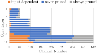
Figure 3: Distribution of channel types across different layers. The ratio of pruned channels in 16th layer is much larger than those in other layers.

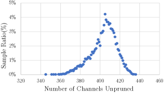
Figure 4: Distribution of unpruned channels in the last block of ResNet-18 w.r.t. samples. It is noticed that the number of unpruned channels varies much among samples.

Though SANP outperforms its variants, it is still wondered that how the distribution of pruned channels look like. It is possible that the pruning rates are same for different layers and it is also possible that the pruned channels are same for all input samples. To answer the above questions, we investigate the pruning strategies generated by SANP. We conduct forward propagation of ResNet-18 in Table 3 and collect the channel pruning decisions generated by SPMs for all samples in CIFAR-10 test set. Then we divide channels into three categories: channels that are never pruned, channels that are pruned dependent on input sample, channels that are always pruned.

Figure 4 shows the distribution of three types of channels. It could be clearly seen that the pruning rate varies across layers and many channels are pruned dependent on input samples, especially channels in deep layers. We also investigate how many channels are utilized with regard to input samples. Figure 4 illustrates the distribution, which indicates that the channel pruning varies much based on input samples.

6 Conclusion

We propose a novel method SANP for channel pruning. Our method adaptively adjusts pruning strategy for each layer according to the input samples, which enables better pruning rate and classification performance. With a differentiable design, our adaptive method can be jointly trained by classification and cost objectives, and thus maximize performance under the computational cost budget. Experiments on CIFAR-10 and CIFAR-100 show that our method achieves state-of-the-art performance over existing methods.

References

- Chollet (2017) François Chollet. Xception: Deep learning with depthwise separable convolutions. In Proceedings of the IEEE conference on computer vision and pattern recognition, pp. 1251–1258, 2017.
- Courbariaux et al. (2016) Matthieu Courbariaux, Itay Hubara, Daniel Soudry, Ran El-Yaniv, and Yoshua Bengio. Binarized neural networks: Training deep neural networks with weights and activations constrained to+ 1 or-1. arXiv preprint arXiv:1602.02830, 2016.
- Du et al. (2019) Simon S Du, Xiyu Zhai, Barnabas Poczos, and Aarti Singh. Gradient descent provably optimizes over-parameterized neural networks. In International Conference on Learning Representations, 2019.
- Gao et al. (2019) Xitong Gao, Yiren Zhao, Lukasz Dudziak, Robert Mullins, and Cheng-zhong Xu. Dynamic channel pruning: Feature boosting and suppression. In International Conference on Learning Representations, 2019.
- Girshick et al. (2014) Ross Girshick, Jeff Donahue, Trevor Darrell, and Jitendra Malik. Rich feature hierarchies for accurate object detection and semantic segmentation. In Proceedings of the IEEE conference on computer vision and pattern recognition, pp. 580–587, 2014.
- Han et al. (2016) Song Han, Huizi Mao, and William J Dally. Deep compression: Compressing deep neural networks with pruning, trained quantization and huffman coding. In International Conference on Learning Representations, 2016.
- He et al. (2016) Kaiming He, Xiangyu Zhang, Shaoqing Ren, and Jian Sun. Deep residual learning for image recognition. In Proceedings of the IEEE conference on computer vision and pattern recognition, pp. 770–778, 2016.
- Hu et al. (2018) Jie Hu, Li Shen, and Gang Sun. Squeeze-and-excitation networks. In Proceedings of the IEEE conference on computer vision and pattern recognition, pp. 7132–7141, 2018.
- Hua et al. (2018) Weizhe Hua, Christopher De Sa, Zhiru Zhang, and G Edward Suh. Channel gating neural networks. In Proceedings of the 55th Annual Design Automation Conference, 2018.
- Huang et al. (2017) Gao Huang, Zhuang Liu, Laurens Van Der Maaten, and Kilian Q Weinberger. Densely connected convolutional networks. In Proceedings of the IEEE conference on computer vision and pattern recognition, pp. 4700–4708, 2017.
- Kaiser & Bengio (2018) Łukasz Kaiser and Samy Bengio. Discrete autoencoders for sequence models. arXiv preprint arXiv:1801.09797, 2018.
- Kaiser & Sutskever (2015) Łukasz Kaiser and Ilya Sutskever. Neural gpus learn algorithms. arXiv preprint arXiv:1511.08228, 2015.
- Krizhevsky & Hinton (2009) Alex Krizhevsky and Geoffrey Hinton. Learning multiple layers of features from tiny images. Technical report, Citeseer, 2009.
- Krizhevsky et al. (2012) Alex Krizhevsky, Ilya Sutskever, and Geoffrey E Hinton. Imagenet classification with deep convolutional neural networks. In Advances in neural information processing systems, pp. 1097–1105, 2012.
- Li et al. (2017) Hao Li, Asim Kadav, Igor Durdanovic, Hanan Samet, and Hans Peter Graf. Pruning filters for efficient convnets. In International Conference on Learning Representations, 2017.
- Lin et al. (2017) Ji Lin, Yongming Rao, Jiwen Lu, and Jie Zhou. Runtime neural pruning. In Advances in Neural Information Processing Systems, pp. 2181–2191, 2017.
- Liu & Deng (2018) Lanlan Liu and Jia Deng. Dynamic deep neural networks: Optimizing accuracy-efficiency trade-offs by selective execution. In Thirty-Second AAAI Conference on Artificial Intelligence, 2018.
- Liu et al. (2017) Zhuang Liu, Jianguo Li, Zhiqiang Shen, Gao Huang, Shoumeng Yan, and Changshui Zhang. Learning efficient convolutional networks through network slimming. In Proceedings of the IEEE International Conference on Computer Vision, pp. 2736–2744, 2017.
- Long et al. (2015) Jonathan Long, Evan Shelhamer, and Trevor Darrell. Fully convolutional networks for semantic segmentation. In Proceedings of the IEEE conference on computer vision and pattern recognition, pp. 3431–3440, 2015.
- Luo & Wu (2018) Jian-Hao Luo and Jianxin Wu. Autopruner: An end-to-end trainable filter pruning method for efficient deep model inference. arXiv preprint arXiv:1805.08941, 2018.
- Ma et al. (2018) Ningning Ma, Xiangyu Zhang, Hai-Tao Zheng, and Jian Sun. Shufflenet v2: Practical guidelines for efficient cnn architecture design. In Proceedings of the European Conference on Computer Vision (ECCV), pp. 116–131, 2018.
- Micikevicius et al. (2018) Paulius Micikevicius, Sharan Narang, Jonah Alben, Gregory Diamos, Erich Elsen, David Garcia, Boris Ginsburg, Michael Houston, Oleksii Kuchaiev, Ganesh Venkatesh, et al. Mixed precision training. In International Conference on Learning Representations, 2018.
- Simonyan & Zisserman (2014) Karen Simonyan and Andrew Zisserman. Very deep convolutional networks for large-scale image recognition. arXiv preprint arXiv:1409.1556, 2014.
- Zhang et al. (2018) Xiangyu Zhang, Xinyu Zhou, Mengxiao Lin, and Jian Sun. Shufflenet: An extremely efficient convolutional neural network for mobile devices. In Proceedings of the IEEE Conference on Computer Vision and Pattern Recognition, pp. 6848–6856, 2018.
- Zhao et al. (2018) Yiren Zhao, Xitong Gao, Robert Mullins, and Chengzhong Xu. Mayo: A framework for auto-generating hardware friendly deep neural networks. In Proceedings of the 2nd International Workshop on Embedded and Mobile Deep Learning, pp. 25–30. ACM, 2018.
- Zhou et al. (2016) Shuchang Zhou, Yuxin Wu, Zekun Ni, Xinyu Zhou, He Wen, and Yuheng Zou. Dorefa-net: Training low bitwidth convolutional neural networks with low bitwidth gradients. arXiv preprint arXiv:1606.06160, 2016.
- Zhou et al. (2018) Zhengguang Zhou, Wengang Zhou, Houqiang Li, and Richang Hong. Online filter clustering and pruning for efficient convnets. In 2018 25th IEEE International Conference on Image Processing (ICIP), pp. 11–15. IEEE, 2018.