High-dimensional and universally consistent k-sample tests

Abstract

The k-sample testing problem involves determining whether $k$ groups of data points are each drawn from the same distribution. The standard method for k-sample testing in biomedicine is Multivariate analysis of variance (Manova), despite that it depends on strong, and often unsuitable, parametric assumptions. Moreover, independence testing and k-sample testing are closely related, and several universally consistent high-dimensional independence tests such as distance correlation (Dcorr) and Hilbert-Schmidt-Independence-Criterion (Hsic) enjoy solid theoretical and empirical properties. In this paper, we prove that independence tests achieve universally consistent k-sample testing and that k-sample statistics such as Energy and Maximum Mean Discrepancy (Mmd) are precisely equivalent to Dcorr. An empirical evaluation of nonparametric independence tests showed that they generally perform better than the popular Manova test, even in Gaussian distributed scenarios. The evaluation included several popular independence statistics and covered a comprehensive set of simulations. Additionally, the testing approach was extended to perform multiway and multilevel tests, which were demonstrated in a simulated study as well as a real-world fMRI brain scans with a set of attributes.

1 Introduction

With the increase in the amount of high-dimensional data in scientific studies, it is increasingly important to discover and decipher nonlinear relationships within those data. One critical question that often comes up is whether two or more groups have the same underlying distribution or not. This is known as the k-sample testing problem. Consider the two-sample problem: given two datasets $u_{i}\in\mathbb{R}^{p}$ for $i=1,\ldots,n$ and $v_{j}\in\mathbb{R}^{p}$ for $j=1,\ldots,m$, assume each $u_{i}$ is sampled independently and identically (i.i.d.) from $F_{U}$ and that each $v_{j}$ is sampled i.i.d. from $F_{V}$ (and also that each $u_{i}$ and each $v_{j}$ is independent from one another). The two-sample testing problem tests whether the two datasets were sampled from the same distribution, that is,

$$\begin{split}H_{0}&:F_{U}=F_{V},\\ H_{A}&:F_{U}\neq F_{V}.\end{split}$$

The k-sample testing problem is a generalization of the above: let $u_{i}^{j}\in\mathbb{R}^{p}$ for $j=1,\dots,k$ and $i=1,\ldots,n_{j}$ be $k$ datasets that are sampled i.i.d. from $F_{1},\ldots,F_{k}$ and independently from one another. Then,

$$\begin{split}H_{0}&:F_{1}=F_{2}=\cdots=F_{k},\\ H_{A}&:\exists\ j\neq j^{\prime}\text{ s.t. }F_{j}\neq F_{j^{\prime}}\end{split}$$

Student’s t-test [1] and its multivariate generalization Hotelling’s $T^{2}$ [2] are traditionally used for two-sample testing, while analysis of variance (Anova) [3] or multivariate Anova (Manova) [4] are conventional choices for k-sample tests. These tests, however, often do not perform well for high-dimensional or non-Gaussian data, because their performance depends on assumptions that are not generally present in real data [5, 6]. A number of nonparametric alternatives have been developed to address this issue, most notably the Energy [7] and maximal mean discrepancy (Mmd) [8] for two-sample test, and multivariate Heller Heller Gorfine [9] and distance components (Disco) [10] for k-sample test.

A closely-related problem is testing independence: given $x_{i}\in\mathbb{R}^{p}$ and $y_{i}\in\mathbb{R}^{q}$, and $n$ samples of $(x_{i},y_{i})\overset{iid}{\sim}F_{XY}$, the independent hypothesis is stated as

$$\begin{split}H_{0}&:F_{XY}=F_{X}F_{Y},\\ H_{A}&:F_{XY}\neq F_{X}F_{Y}.\end{split}$$

The traditional Pearson’s correlation [11] is still very popular, but it is only limited to detect linear dependence. Many non-parametric methods have been proposed, such as distance correlation (Dcorr) [12, 13, 14, 15], Hilbert-Schmidt independence criterion (Hsic) [16, 17, 18], Hhg method [19], Multiscale Graph Correlation (Mgc) [20, 21, 22], ball covariance [23], Kernel Mean Embedding Random Forest (Kmerf) [24], among many others. Those recent dependence measures are universally consistent, thus they are able to asymptotically detect any type of relationship, not just linear. However, there is no uniformly most powerful test for general Independence settings.

In this manuscript, we illustrate a fundamental connection between k-sample testing and independence testing, and provide guidance on a broad range of tests. We prove that any consistent independence tests can be used for consistent k-sample testing, including multiway and multilevel generalizations of k-sample testing. We then establish the equivalence between the Energy and Dcorr, as well as the equivalence between Mmd and Hsic. Empirically, we evaluate these independence tests in k-sample testing scenarios. The results indicate that these independence tests yield higher statistical power than conventional Manova in a number of settings, including Gaussian settings with low-sample size. In additional, we demonstrate how to extend our existing k-sample testing framework to include multiway and multilevel tests, and apply it to simulated and real-world fMRI brain scans. All the code and k-sample tests are provided in the hyppo statistical package [22] and available on GitHub.

2 Main Results

In this section, we present the main method and theory contributions. The proofs and certain technical details (like the mathematical formulation of Energy and Mmd) are in the appendix.

2.1 Independence Tests for K-Sample Testing

K-sample testing can be carried out by independence tests as follows: consider $\boldsymbol{u}_{1},\ldots,\boldsymbol{u}_{k}$ as matrices of size $n_{1}\times p,\ldots,n_{k}\times p$, where $p$ refers to the number of dimensions and $n_{i}$ refers to the number of samples of $\boldsymbol{u}_{i}$. Let $n=\sum_{i=1}^{k}n_{i}$. In the case where $n=2$, we can define the data matrices $\boldsymbol{x}$ and $\boldsymbol{y}$ by

$$\boldsymbol{x} =\begin{bmatrix}\boldsymbol{u}_{1}\\ \boldsymbol{u}_{2}\end{bmatrix}\in\mathbb{R}^{n\times p},$$

$$\boldsymbol{y} =\begin{bmatrix}\boldsymbol{0}_{n_{1}\times 1}\\ \boldsymbol{1}_{n_{2}\times 1}\end{bmatrix}\in\mathbb{R}^{n}.$$

For $n>2$, $\boldsymbol{y}$ is a one-hot encoding of $\boldsymbol{x}$. That is,

$$\boldsymbol{x} =\begin{bmatrix}\boldsymbol{u}_{1}\\ \vdots\\ \boldsymbol{u}_{k}\end{bmatrix}\in\mathbb{R}^{n\times p},$$

$$\boldsymbol{y} =\begin{bmatrix}\boldsymbol{1}_{n_{1}\times 1}&\boldsymbol{0}_{n_{1}\times 1}&\ldots&\boldsymbol{0}_{n_{1}\times 1}\\ \boldsymbol{0}_{n_{2}\times 1}&\boldsymbol{1}_{n_{2}\times 1}&\ldots&\boldsymbol{0}_{n_{2}\times 1}\\ \vdots&\vdots&\ddots&\vdots\\ \boldsymbol{0}_{n_{k}\times 1}&\boldsymbol{0}_{n_{k}\times 1}&\ldots&\boldsymbol{1}_{n_{k}\times 1}\\ \end{bmatrix}\in\mathbb{R}^{n\times k}.$$

Here, $\boldsymbol{x}$ is the concatenated data matrix contains all the $\{\boldsymbol{u}_{i}\}$, while $\boldsymbol{y}$ is the auxiliary label matrix indicating which data source every observation comes from. Now $\boldsymbol{x}$ and $\boldsymbol{y}$ are paired data matrices, and one may use any dependence measure on this pair.

2.2 Multiway and Multilevel Generalization

The above k-sample data to independence pair transformation can be further extended for a multiway test where samples have multiple labels.

Let $\boldsymbol{y}$ be formulated as follows: given $\boldsymbol{u}$ as defined above, to perform a $w$-way test, where $w<k$, each row of $\boldsymbol{y}$ contains $w$ $\boldsymbol{1}_{n_{i}}$ elements. These $\boldsymbol{1}_{n_{i}}$ elements can be in any of the $k$ columns of $\boldsymbol{y}$. For example, one possible way to perform a $w$-way test is,

$$\boldsymbol{y}=\begin{bmatrix}\boldsymbol{1}_{n_{1}\times 1}&\boldsymbol{0}_{n_{1}\times 1}&\ldots&\boldsymbol{1}_{n_{1}\times 1}\\ \boldsymbol{1}_{n_{2}\times 1}&\boldsymbol{1}_{n_{2}\times 1}&\ldots&\boldsymbol{0}_{n_{2}\times 1}\\ \vdots&\vdots&\ddots&\vdots\\ \boldsymbol{0}_{n_{k}\times 1}&\boldsymbol{1}_{n_{k}\times 1}&\ldots&\boldsymbol{1}_{n_{k}\times 1}\\ \end{bmatrix}\in\mathbb{R}^{n\times k}.$$

Performing a multilevel test involves constructing $x$ and $y$ using either of the methods above and then performing a block permutation [25]. Essentially, the permutation is striated, where permutation is limited to be within a block of samples or between blocks of samples, but not both. This is done because the data is not freely exchangeable, so it is necessary to block the permutation to preserve the joint distribution [25].

2.3 Supporting Theory

Lemma 2.1.

Let $Y\in\mathbb{R}^{k}$ be the $1$-trial multinomial distribution of probability $(\pi_{1},\pi_{2},\ldots,\pi_{k})$ where $\pi_{l}=\frac{n_{l}}{n}$, and $X$ be the following mixture:

$$X\stackrel{{\scriptstyle d}}{{=}}\sum_{l=1}^{k}U_{l}I(Y(l)\neq 0),$$

where $U_{l}$ is the underlying random variable for each $\boldsymbol{u}_{l}$ and $I(\cdot)$ is the indicator function. Then $X$ is independent of $Y$ if and only if $U_{1}\stackrel{{\scriptstyle d}}{{=}}U_{2}\stackrel{{\scriptstyle d}}{{=}}\cdots\stackrel{{\scriptstyle d}}{{=}}U_{k}$.

Namely, any method that is universally consistent for testing independence between $\boldsymbol{x}$ and $\boldsymbol{y}$ is also universally consistent for a k-sample test. Interestingly, distance covariance applied to the transformed $(\boldsymbol{x},\boldsymbol{y})$ is exactly the same as the two-sample energy statistic between $\boldsymbol{u}_{1}$ and $\boldsymbol{u}_{2}$.

Theorem 2.2.

Assume both distance covariance and energy statistic use a same translation invariant metric $d(\cdot,\cdot)$. Denote $\beta=d(0,1)-d(0,0)$, it follows that

$$\text{{\sc{Dcov}}}_{n}(\boldsymbol{x},\boldsymbol{y})=\frac{2n_{1}^{2}n_{2}^{2}\beta}{n^{4}}\cdot\text{{\sc{Energy}}}_{n_{1},n_{2}}(\boldsymbol{u}_{1},\boldsymbol{u}_{2}),$$

Under the permutation test, distance covariance, distance correlation, and energy statistic have the same testing p-value.

Due to the equivalence between distance and kernel [26, 27], the Hilbert-Schmidt independence criterion is also the same as the maximum mean discrepancy.

Lemma 2.3.

Assume both Hilbert-Schmidt independence criterion and maximum mean discrepancy use a same translation-invariant kernel $k(\cdot,\cdot)$. Denote $\beta=k(0,1)-k(0,0)$, it follows that

$$\text{{\sc{Hsic}}}_{n}(\boldsymbol{x},\boldsymbol{y})=\frac{2n_{1}^{2}n_{2}^{2}\beta}{n^{4}}\cdot\text{{\sc{Mmd}}}_{n_{1},n_{2}}(\boldsymbol{u}_{1},\boldsymbol{u}_{2}),$$

Under the permutation test, Hilbert-Schmidt independence criterion and maximum mean discrepancy have the same testing p-value.

Lastly, we establish a relationship between distance covariance and k-sample Energy, proposed in [10], which consist of the same number of pairwise energy components but weight them differently.

Theorem 2.4.

Assume both distance covariance and k-sample energy statistic use a same translation invariant metric $d(\cdot,\cdot)$. Denote $\beta=d(\boldsymbol{y}(s,:),\boldsymbol{y}(t,:))-d(\boldsymbol{y}(s,:),\boldsymbol{y}(s,:))$ for some $s\neq t$, it follows that

$$\text{{\sc{Dcov}}}_{n}(\boldsymbol{x},\boldsymbol{y})=\beta\sum_{1\leq s<t\leq k} \left\{\frac{n(n_{s}+n_{t})-\sum_{l=1}^{k}n_{l}^{2}}{n^{4}}\cdot n_{s}n_{t}\text{{\sc{Energy}}}_{n_{s},n_{t}}(\boldsymbol{u}_{s},\boldsymbol{u}_{t})\right\}.$$

Distance covariance and k-sample energy statistic become the same if and only if either $k=2$, or $n_{1}=n_{2}=\ldots=n_{k}$, in which case

$$\text{{\sc{Dcov}}}_{n}(\boldsymbol{x},\boldsymbol{y})=\frac{2\beta}{nk}\text{{\sc{Energy}}}_{n_{1},\ldots,n_{k}}(\{\boldsymbol{u}_{k}\}).$$

3 Empirical Analysis

3.1 Gaussian Simulations

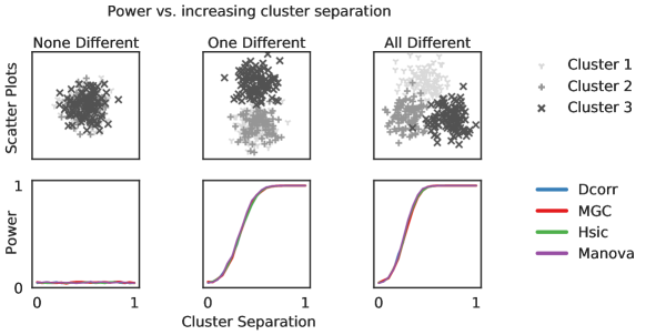
Figure 1: The figure displays power versus epsilon curves for three different parameter settings using the generated two-dimensional Gaussian dataset with 100 samples for each of the four cases. The top row shows a scatter plot of each simulation, while the bottom row shows the power curves for each simulation with an increasing cluster separation (averaged over 5 replicates).

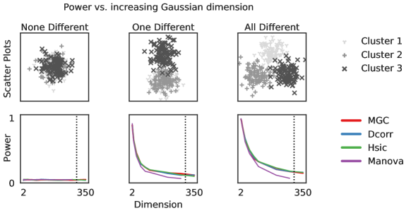
Figure 2: This figure shows the power versus dimension curves for three different parametric settings, with a fixed sample size of 100 and epsilon of $0.5$.

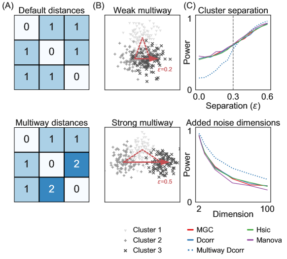
Figure 3: This figure compares different simulation settings for multiway and one-way tests. (A) Multiway tests are created using one-hot encoding for label matrices. (B) Three two-dimensional Gaussians are shown, with means forming an isosceles triangle and two values of $\epsilon$ (0.2 and 0.5) for visualization purposes. Weak multiway effects are expected when $\epsilon<c$ (top) and strong multiway effects are expected when $\epsilon>c$ (bottom). (C) At a fixed sample size of 100 and dimension of 2.

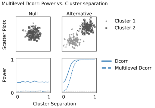
Figure 4: This figure shows power versus epsilon curves for regular and multilevel Dcorr  in a multilevel setting. To create the data, 100 means were sampled from each two-dimensional Gaussian, and two samples were generated from Gaussians centered at each mean and with lower variance (400 samples total). The top row presents a scatter plot of each simulation for a given cluster separation, and the bottom row shows the power curves for each simulation as cluster separation increases (averaged over 5 replicates).

We consider three basic three-sample tests with Gaussian distributions and an identity covariance matrix ($I$):

1. None Different, where all three groups have the same mean of $\mu=(0,0)$.

2. One Different, where two groups have the same mean of $\mu=(0,0)$ and the third group has a different mean of $\mu=(0,\epsilon)$.

3. All Different, where the means of the three groups form an equilateral triangle centered at $(0,0)$ and with a radius of $\epsilon$. Specifically, $\mu_{1}=(0,\sqrt{3}/3\times\epsilon)$, $\mu_{2}=(-\epsilon/2,-\sqrt{3}/6\times\epsilon)$, and $\mu_{3}=(\epsilon/2,-\sqrt{3}/6\times\epsilon)$.

Figure 1 shows the scatter plots and statistical power for these three different cases of two-dimensional Gaussians as $\epsilon$ increases from 0 to 1. The test results for None Different show proper type I error control for all tests, yielding a power no greater than $\alpha$ (set to 0.05). For One Different and All Different, where the distributions have increased separation, all four tests (k-sample Dcorr, Hsic, Mgc, and Manova) perform equally well, despite this being an ideal setting for Manova.

In Figure 2, we explore the same simulations, but instead fix $\epsilon=0.5$ and vary the dimension of each Gaussian from 2 to 100. To do this, we simulated a two-dimensional Gaussian at the fixed $\epsilon$ and added additional uninformative features drawn from a standard normal distribution. As the dimension increases, the statistical power is expected to decrease. In the None Different case, we confirm that each test controls type I error properly. In the One Different and All Different cases, we observe that Mgc, Dcorr, and Hsic outperform Manova(columns 2 and 3), particularly as the sample size approaches the number of dimensions. It should be noted that Manova does not work when the dimension exceeds the rank, which is at most equal to the sample size (300 in this simulation, marked by the vertical dashed line).

Figure 3 investigates the nature of the multiway effect and the ideal settings for performing multiway tests. The label matrices (row A) illustrate how the pairwise distance matrix is computed, with each block being $n_{i}\times n_{i}$, where $n_{i}$ is the number of samples for each cluster (100 in these simulations). To investigate the performance of multiway tests, we simulated three two-dimensional Gaussians with means forming a triangle: one at the origin and the other two fixed distances ($c$) away from the origin, separated by a variable distance ($\epsilon$). The means were defined as $\mu_{1}=(0,0)$, $\mu_{2}=(-\epsilon/2,-\sqrt{c^{2}-(\epsilon/2)^{2}})$, and $\mu_{3}=(\epsilon/2,-\sqrt{c^{2}-(\epsilon/2)^{2}})$, and the covariance matrix was the identity matrix. When the two variable Gaussians are more different from each other than the Gaussian at the origin (i.e., $\epsilon>c$), the assumed multiway label matrix hierarchy in Figure 3 matches the true hierarchy. When the two variable Gaussians are more similar to each other (i.e., $\epsilon<c$), the assumed hierarchy is incorrect.

We set $c=0.3$ and varied the separation ($\epsilon$) from $0$ to $0.6$ to investigate the nature of the multiway effect in Figure 3. When the separation was less than $c$, we observed a decrease in power, indicating that the multiway assumption was false (row B, left). Conversely, when the separation was greater than $c$, we observed an increase in power, indicating that the multiway assumption was true (row B, right). The multiway test statistic is larger or smaller than the one-way statistic under the alternative hypothesis depending on whether the multiway assumption is true or false. In row C, we fixed the dimension at two and increased the separation (left) and dimension (right). For small cluster separations, the power of multiway Dcorr was low, but it became at or above the power of all other tests when the separation exceeded $c$, consistent with our expectations. At $\epsilon=0.5>c$ and the dimension was increased, multiway Dcorr clearly dominated all other tests at all dimensions.

Figure 4 illustrates that non-multilevel Dcorr is not a valid statistic in the multilevel setting. In this simulation, we sampled 100 means from each of two Gaussians with covariance equal to the identity matrix ($\mathcal{N}(0,1)$ and $\mathcal{N}(\varepsilon,1)$) at a fixed distance from each other. Two samples were drawn from each mean $\mu$ from a Gaussian with variance $0.1$ around the mean ($\mathcal{N}(\mu,0.1)$). Under the null, where cluster separation is 0, regular Dcorr achieves power greater than the $\alpha$-level, making it an invalid procedure. In contrast, multilevel Dcorr is a valid statistic (power equals $\alpha$) because its permutations reflect proper exchangeability of samples under the null [25]. Although non-multilevel Dcorr has higher power than its multilevel counterpart, this is merely an artifact of its invalidity in this setting.

These findings suggest that nonparametric k-sample tests can perform just as well as the Manova test, and sometimes even better, even in Gaussian settings. For instance, in high-dimensional multiway testing, k-sample tests may outperform the Manova test, despite the latter being expected to perform better in a linear simulation setting where all distributions are Gaussian and have the same covariance.

3.2 A Benchmark Suite of 20 Rotated Simulations for K-Sample Testing

We evaluate a benchmark suite of 20 different distributions previously developed for independence testing, including polynomial (linear, quadratic, cubic), trigonometric (sinusoidal, circular, ellipsoidal, spiral), geometric (square, diamond, W-shaped), and other relationships [28, 19, 22, 29, 14, 12, 21]. For each case, we draw $n$ samples from one of the 20 different distributions, rotate the distribution counter-clockwise to generate a second sample, and rotate the distribution clockwise to form a third sample. The noise distribution is determined as described in Vogelstein et al. [21]. The power curves for each of the 20 settings are shown in the following three figures. The bottom right panel demonstrates the power under the null, which must be less than or equal to $\alpha$ for the test to be valid.

Figure 5 evaluates the tests in three-sample tests with two-dimensional distributions $x$, $y$, and $z$, where $F_{y}$ is rotated 90 degrees counterclockwise relative to $F_{x}$ and $F_{z}$ is rotated 90 degrees clockwise relative to $F_{x}$, for varying sample sizes. In this setting, k-sample Mgc and k-sample Kmerf perform as well as, or better than, all other k-sample tests across all simulation settings and sample sizes, while maintaining proper Type I error control. Additionally, Manova performs similarly to k-sample Cca and k-sample RV. Notably, all of the nonparametric k-sample tests we evaluate outperform Manova, even in the linear and Gaussian settings.

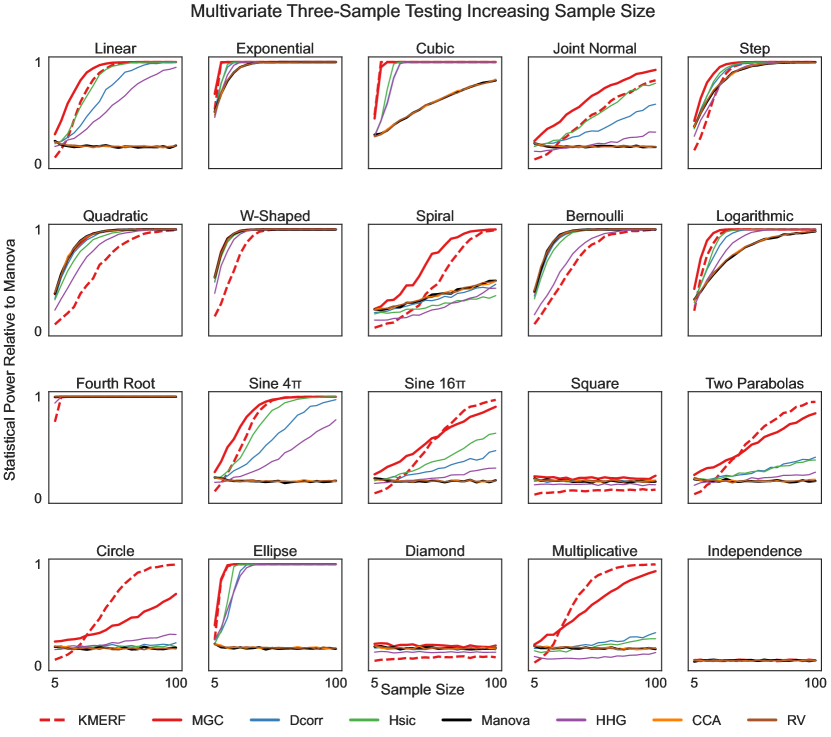
Figure 5: This figure presents power versus sample size curves for 20 three-sample simulations with a fixed angle of 90 degrees, where all inputs are two-dimensional. It is worth noting that the noise applied to the circle simulation is not isotropic.

Figure 6 shows the same 20 settings, except the sample size is fixed at $n=100$ the rotation angle for $F_{y}$ and $F_{z}$ is varied from $0^{\circ}$ to $90^{\circ}$. As with Figure 5, power was plotted relative to Manova. In this setting, for nearly all angles and simulation settings, k-sample Mgc and k-sample Kmerf achieved the same or higher power when compared to every other test in nearly all settings.

Figure 7 shows the power of these tests as the number of dimensions increases, while keeping the sample size and rotation angle fixed at 100 samples per group and 90 degrees, respectively. In this setting, k-sample Mgc and Kmerf outperform every other test in nearly all settings again.

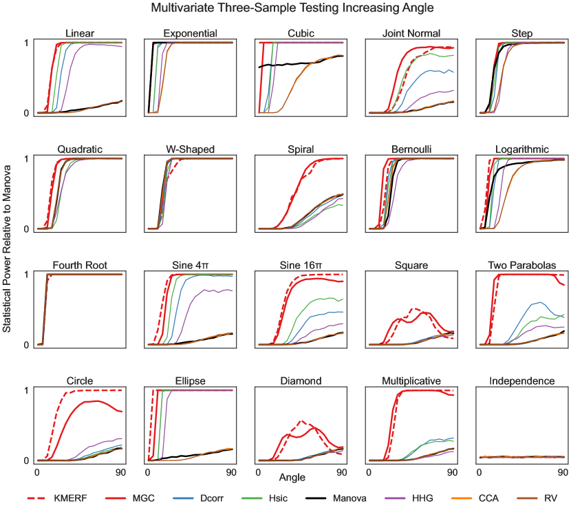
Figure 6: This figure displays power curves of 20 three-sample tests with a fixed sample size of 100 samples and two dimensions, for a range of angles (averaged over 5 replicates). The tests were conducted to evaluate the performance of various methods, including k-sample Mgc and Kmerf.

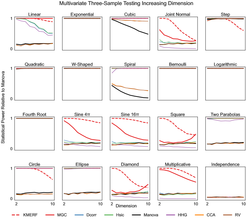
Figure 7: This figure displays power versus dimension for 20 three-sample simulations in three-dimensions with fixed sample size (100 samples) and angle (90 degrees) averaged over 5 replicates. The results show that k-sample Mgc and Kmerf dominate the other tests in nearly all of the simulation settings in terms of achieving higher statistical power.

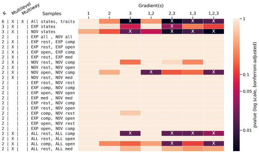
Figure 8: The figure shows the results of omnibus and pairwise tests performed on combinations of states (open, rest, comp) and traits (NOV, EXP), with significant corrected p-values (indicated by a white X) at the $0.05-\alpha$ level.

4 Real data experiment: fMRI measurements

In this fMRI data analysis, the multiway and multilevel effects were investigated using Dcorr. The data consisted of 75 subjects, including 28 experienced meditators who had more than ten thousand hours of practice each and 47 novice meditators who had only one weekend of training. Each subject underwent three recording sessions: one at resting state, one during an open monitoring meditative state, and one during a compassion meditative state. The fMRI data were preprocessed using the standard fmriprep [30] pipeline and projected onto the fsaverage5 [31] surface meshes, resulting in a time-series of between 200 and 300 timesteps across 18715 cortical vertices for each of the 225 subject scans.

The low dimensional embeddings of the fMRI scans, or "gradients," were calculated using generalized canonical correlation analysis (GCCA) [32, 33, 34] from the mvlearn Python package, functionally similar to group PCA [35]. This technique maximizes the sum of pairwise correlations across cortical vertices to find embeddings for each scan, which are effectively aligned. The top three gradients were calculated for each subject. The goal of this analysis was to test for differences in the embeddings between different states and traits, such as recording task and expertise level.

We conducted a multisample, multilevel analysis of the top three GCCA embedding dimensions. A six-sample multiway test was performed on each embedding as well as a combination of them into a single vector, and two subsequent three-sample tests were performed within the novice and expert groups, separately, as well as two-sample tests of interest. Because of repeat measurements from the same subject in some of the tests, a strong within-subject effect dominated and so a multilevel permutation-correction was applied to yield a valid test at the $\alpha=0.05$ level. As multiple hypothesis tests were conducted, in each k-sample stage we applied the conservative Bonferroni correction [36], adjusting our p-values by the number of tests run, up to and including that stage. Figure 8 illustrates that significant differences were found between all subjects during the resting state and compassion, during compassion and open monitoring, and between novice meditators in compassion and open monitoring. The six-sample test showed significant effects from the third embedding and its combinations. Further, subsequent three-sample and two-sample tests revealed significant differences, primarily within novice meditators and between the compassion meditative state, with respect to the third embedding.

5 Conclusion

We presented a set of independent statistics for k-sample testing, and established the equivalence between independence and k-sample testing. The proposed transformation of k-sample data to independence pairs is sufficiently general to work for any independence statistic, current or future. We demonstrated the utility of this transformation by showing that some nonparametric k-sample tests performed slightly better than Manova in settings where Manova was expected to perform best, and that k-sample Mgc outperformed all other k-sample tests across a wide range of dependency structures.

We expanded our k-sample testing approach to include multiway and multilevel tests. In scenarios where one effect dominates the others, multiway tests perform as well as or better than state-of-the-art tests at low dimensions and outperform them as dimensionality increases. We also applied our multiway and multilevel tests to large real-world data where Manova was computationally infeasible, and were able to identify significant differences in multiple embeddings between different states. Notably, our approach does not increase computational complexity beyond that of the desired independence test.

Overall, our results suggest that there are many more k-sample tests available than previously thought, and that the proposed approach can be used to leverage the finite-sample testing power of new independence tests to create even more powerful k-sample tests in the future.

Data and Code Availability Statement

The analysis and visualization of this data were done using the hyppo open-source package https://hyppo.neurodata.io/ and the mvlearn package https://mvlearn.github.io/. Source code, documentation, and tutorials can be found there.

Acknowledgements

This work is graciously supported by the Defense Advanced Research Projects Agency (DARPA) Lifelong Learning Machines program through contract FA8650-18-2-7834, the National Institute of Health awards RO1MH120482 and T32GM119998, and the National Science Foundation award DMS-1921310 and DMS-2113099, and Microsoft Research. The authors would also like to acknowledge Dr. Russell Lyons, Dr. Minh Tang, Mr. Ronak Mehta, Mr. Eric W. Bridgeford, and the rest of the NeuroData family at Johns Hopkins University for helpful feedback throughout the development process.

APPENDIX

Appendix A Supplementary Information

The analysis and visualization of this data were done using the hyppo open-source package https://hyppo.neurodata.io/ and the mvlearn package https://mvlearn.github.io/. Source code, documentation, and tutorials can be found there. Figure replication code for this manuscript can be found here: https://github.com/neurodata/hyppo-papers/tree/main/ksample.

Appendix B Preliminaries

B.1 Notation

Let $\mathbb{R}$ denote the real line $(-\infty,\infty)$. Let $F_{X}$, $F_{Y}$, and $F_{XY}$ refer to the marginal and joint distributions of random variables $X$ and $Y$ respectively. Let $x$ and $y$ refer to the samples from $F_{X}$ and $F_{Y}$, and $\boldsymbol{x}\in\mathbb{R}^{n\times p}$ and $\boldsymbol{y}\in\mathbb{R}^{m\times p}$ such that $\boldsymbol{x}=\{x_{1},\ldots,x_{n}\}$ and $\boldsymbol{y}=\{y_{1},\ldots,y_{m}\}$. The trace of an $n\times n$ square matrix is the sum of the elements along the main diagonal: ${\operatorname{tr}\!\left(\boldsymbol{x}\right)}=\sum_{i=1}^{n}x_{ii}$.

B.2 Manova

Manova is a procedures for comparing more than two multivariate samples [37, 6]. It is a multivariate generalization of the univariate Anova [6] using covariance matrices rather than the scalar variances. As in [38]: consider input samples $\boldsymbol{x}_{1},\boldsymbol{x}_{2},\ldots,\boldsymbol{x}_{k}$ that have the same dimensionality $p$. Each $\boldsymbol{x}_{i}$, where $i\in\{1,\ldots,k\}$ is assumed to be sampled from a multivariate distribution $\mathbb{N}(\boldsymbol{\mu}_{i},\boldsymbol{\Sigma})$ and so each sample is assumed to have the same covariance matrix $\boldsymbol{\Sigma}$. The model for each $p$-dimensional vector of each $\boldsymbol{x}_{i}$ is defined as follows: for $j\in\{1,\ldots,n_{i}\}$,

$$\boldsymbol{x}_{ij}=\boldsymbol{\mu}_{i}+\boldsymbol{\epsilon}_{ij}.$$

In Manova, we are testing if the mean vectors of each of the k-samples are the same. That is, the null and alternate hypotheses are,

$$H_{0} :\boldsymbol{\mu}_{1}=\boldsymbol{\mu}_{2}=\cdots=\boldsymbol{\mu}_{k},$$

$$H_{A} :\exists\ j\neq j^{\prime}\text{ s.t. }\boldsymbol{\mu}_{j}\neq\boldsymbol{\mu}_{j^{\prime}}$$

Let $\bar{\boldsymbol{x}}_{i\cdot}$ refer to the columnwise means of $\boldsymbol{x}_{i}$; that is, $\bar{\boldsymbol{x}}_{i\cdot}=(1/n_{i})\sum_{j=1}^{n_{i}}\boldsymbol{x}_{ij}$. The pooled sample covariance of each group, $\boldsymbol{W}$, is

$$\boldsymbol{W}=\sum_{i=1}^{k}\sum_{j=1}^{n_{i}}(\boldsymbol{x}_{ij}-\bar{\boldsymbol{x}}_{i\cdot})(\boldsymbol{x}_{ij}-\bar{\boldsymbol{x}}_{i\cdot})^{\mathsf{T}}.$$

Next, define $\boldsymbol{B}$ as the sample covariance matrix of the means. If $n=\sum_{i=1}^{k}n_{i}$ and the grand mean is $\bar{\boldsymbol{x}}_{\cdot\cdot}=(1/n)\sum_{i=1}^{k}\sum_{j=1}^{n}\boldsymbol{x}_{ij}$,

$$\boldsymbol{B}=\sum_{i=1}^{k}n_{i}(\bar{\boldsymbol{x}}_{i\cdot}-\bar{\boldsymbol{x}}_{\cdot\cdot})(\bar{\boldsymbol{x}}_{i\cdot}-\bar{\boldsymbol{x}}_{\cdot\cdot})^{\mathsf{T}}.$$

Some of the most common test statistics used when performing Manova include the Wilks’ Lambda, the Lawley-Hotelling trace, Roy’s greatest root, and Pillai-Bartlett trace (PBT) [39, 40, 41] (PBT is recognized to be the best of these as it is the most conservative [42, 6]) and [43] has shown that there are minimal differences in statistical power among these statistics. Let $\lambda_{1},\lambda_{2},\ldots,\lambda_{s}$ refer to the eigenvalues of $\boldsymbol{W}^{-1}\boldsymbol{B}$. Here $s=\min(\nu_{\boldsymbol{B}},p)$ is the minimum between the degrees of freedom of $\boldsymbol{B}$, $\nu_{\boldsymbol{B}}$ and $p$. So, the PBT Manova test statistic [37] can be written as,

$$\begin{aligned} \text{{\sc{Manova}}}_{n_{1},\ldots,n_{k}}(\boldsymbol{x},\boldsymbol{y})&=\sum_{i=1}^{s}\frac{\lambda_{i}}{1+\lambda_{i}}={\operatorname{tr}\!\left(\boldsymbol{B}(\boldsymbol{B}+\boldsymbol{W})^{-1}\right)}.\end{aligned}$$

Since it is a multivariate generalization of Student’s t-tests, it suffers from some of the same assumptions as Student’s t-tests. That is, the validity of Manova depends on the assumption that random variables are normally distributed within each group and each with the same covariance matrix. Distributions of input data are generally not known and cannot always be reasonably modeled as Gaussian [44, 45], and having the same covariance across groups is also generally not true of real data.

B.3 Independence Tests

B.3.1 Dcorr

Dcorr is a powerful test to determine linear and nonlinear associations between two random variables or vectors in arbitrary dimensions. The test statistic can be determined as follows: let $\boldsymbol{D}^{\boldsymbol{x}}$ and ${\boldsymbol{D}}^{\boldsymbol{y}}$ be the $n\times n$ distance matrices of $\boldsymbol{x}$ and $\boldsymbol{y}$. Define $\boldsymbol{H}=\boldsymbol{I}-\frac{1}{n}\boldsymbol{J}$ as a $n\times n$ centering matrix, where $\boldsymbol{I}$ is the identity matrix and $\boldsymbol{J}$ is the matrix of ones. The distance covariance ($\widehat{\text{{\sc{Dcov}}}}$) and distance correlation ($\widehat{\text{{\sc{Dcorr}}}}$) [12] are

$$\widehat{\text{{\sc{Dcov}}}}_{n}(\boldsymbol{x},\boldsymbol{y}) =\frac{1}{n^{2}}{\operatorname{tr}\!\left(\boldsymbol{H}\boldsymbol{D}^{\boldsymbol{x}}\boldsymbol{H}\boldsymbol{H}\boldsymbol{D}^{\boldsymbol{y}}\boldsymbol{H}\right)}.$$

$$\widehat{\text{{\sc{Dcorr}}}}_{n}(\boldsymbol{x},\boldsymbol{y}) =\frac{\widehat{\text{{\sc{Dcov}}}}_{n}(\boldsymbol{x},\boldsymbol{y})}{\sqrt{\widehat{\text{{\sc{Dcov}}}}_{n}(\boldsymbol{x},\boldsymbol{x})\cdot\widehat{\text{{\sc{Dcov}}}}_{n}(\boldsymbol{y},\boldsymbol{y})}}.$$

The statistics presented above are biased. Fortunately, unbiased distance correlation test statistics have also been developed [46]. Define another modified matrix $\boldsymbol{C}^{\boldsymbol{x}}$ such that,

$${\boldsymbol{C}_{ij}}^{\boldsymbol{x}}=\left\{\begin{aligned} &\boldsymbol{D}^{\boldsymbol{x}}_{ij}-\frac{1}{n-2}\sum_{t=1}^{n}\boldsymbol{D}^{\boldsymbol{x}}_{it}-\frac{1}{n-2}\sum_{t=1}^{n}\boldsymbol{D}^{\boldsymbol{x}}_{tj}+\frac{1}{(n-1)(n-2)}\sum_{t=1}^{n}\boldsymbol{D}^{\boldsymbol{x}}_{tt}&&i\neq j\\[4.30554pt] &0&&i=j\end{aligned}\right.$$

and define $\boldsymbol{C}^{\boldsymbol{y}}$ similarly. Then, the unbiased distance covariance (Dcov) and unbiased distance correlation (Dcorr) [46] are

$$\text{{\sc{Dcov}}}_{n}(\boldsymbol{x},\boldsymbol{y}) =\frac{1}{n(n-3)}{\operatorname{tr}\!\left(\boldsymbol{C}^{\boldsymbol{x}}\boldsymbol{C}^{\boldsymbol{y}}\right)}.$$

$$\text{{\sc{Dcorr}}}_{n}(\boldsymbol{x},\boldsymbol{y}) =\frac{\text{{\sc{Dcov}}}_{n}(\boldsymbol{x},\boldsymbol{y})}{\sqrt{\text{{\sc{Dcov}}}_{n}(\boldsymbol{x},\boldsymbol{x})\cdot\text{{\sc{Dcov}}}_{n}(\boldsymbol{y},\boldsymbol{y})}}$$

Since the statistics presented provide similar empirical results to the biased statistics [21], from now on any reference to distance correlation will refer to the unbiased distance correlation.

B.3.2 Hsic

Hilbert-Schmidt independence criterion (Hsic) is a closely related test that exchanges distance matrices $\boldsymbol{D}^{\boldsymbol{x}}$ and $\boldsymbol{D}^{\boldsymbol{y}}$ for kernel similarity matrices $\boldsymbol{K}^{\boldsymbol{x}}$ and $\boldsymbol{K}^{\boldsymbol{y}}$. They are exactly equivalent in the sense that every valid kernel has a corresponding valid semimetric to ensure their equivalence, and vice versa [26, 27]. In other words, every Dcorr test is also an Hsic test and vice versa. nonetheless, implementations of Dcorr and Hsic use different metrics by default: Dcorr uses a Euclidean distance while Hsic uses a Gaussian kernel similarity.

B.3.3 Mgc

Building upon the ideas of Dcorr, Hsic, and k-nearest neighbors, Mgc preserves the consistency property while typically working better in multivariate and non-monotonic relationships [21, 20]. The Mgc test statistic is computed as follows:

1. Two distance matrices $\boldsymbol{D}^{\boldsymbol{x}}$ and $\boldsymbol{D}^{\boldsymbol{y}}$ are computed, and modified to be mean zero column-wise. This results in two $n\times n$ distance matrices $\boldsymbol{C}^{\boldsymbol{x}}$ and $\boldsymbol{C}^{\boldsymbol{y}}$ (the centering and unbiased modification is slightly different from the unbiased modification in the previous section, see [20] for more details).

2. For all values $k$ and $l$ from $1,\ldots,n$,

   1. The $k$-nearest neighbor and $l$-nearest neighbor graphs are calculated for each property. Here, $\boldsymbol{G}_{kij}$ has value 1 for the $k$ smallest values of the $i$-th row of $\boldsymbol{D}^{\boldsymbol{x}}$ and $\boldsymbol{H}_{lij}$ has value 1 the $l$ smallest values of the $i$-th row of $\boldsymbol{D}^{\boldsymbol{y}}$. All other values in both matrices are 0.

   2. The local correlations are summed and normalized using the following statistic:

      $$c^{kl}=\frac{\sum_{ij}\boldsymbol{D}^{\boldsymbol{x}}_{ij}\boldsymbol{G}_{kij}\boldsymbol{D}^{\boldsymbol{y}}_{ij}\boldsymbol{H}_{lij}}{\sqrt{(\boldsymbol{D}^{\boldsymbol{x}}_{ij})^{2}\boldsymbol{G}_{kij}}\cdot\sqrt{(\boldsymbol{D}^{\boldsymbol{y}}_{ij})^{2}\boldsymbol{H}_{lij}}},$$

3. The Mgc test statistic is the smoothed optimal local correlation of $\left\{c^{kl}\right\}$. Denote the smoothing operation as $R(\cdot)$ (which essentially set all isolated large correlations as 0 and connected large correlations same as before, see [20]), Mgc is

   $$\text{{\sc{Mgc}}}_{n}(\boldsymbol{x},\boldsymbol{y})=\max_{(k,l)}R(c^{kl}(\boldsymbol{x}_{n},\boldsymbol{y}_{n})).$$

B.3.4 Kmerf

The Kmerf test statistic is a kernel method for calculating independence by using a random forest induced similarity matrix as an input, and has been shown to have especially high gains in finite sample testing power in high dimensional settings [24]. It is computed using the following algorithm:

1. Run random forest with $m$ trees. Independent bootstrap samples of size $n_{b}\leq n$ are drawn to build a tree each time; each tree structure within the forest is denoted as $\phi_{w}\in\boldsymbol{P}$, $w\in\{1,\ldots,m\}$; $\phi_{w}(x_{i})$ denotes the partition assigned to $x_{i}$.

2. Calculate the proximity kernel:

   $$\boldsymbol{K}^{\boldsymbol{x}}_{ij}=\frac{1}{m}\sum_{w=1}^{m}I(\phi_{w}(x_{i})=\phi_{w}(x_{j})),$$

   where $I(\cdot)$ is the indicator function.

3. Compute the induced kernel correlation: let

   $$\boldsymbol{L}^{\boldsymbol{x}}_{ij}=\left\{\begin{aligned} &\boldsymbol{K}^{\boldsymbol{x}}_{ij}-\frac{1}{n-2}\sum_{t=1}^{n}\boldsymbol{K}^{\boldsymbol{x}}_{it}-\frac{1}{n-2}\sum_{s=1}^{n}\boldsymbol{K}^{\boldsymbol{x}}_{sj}+\frac{1}{(n-1)(n-2)}\sum_{s,t=1}^{n}\boldsymbol{K}^{\boldsymbol{x}}_{st}&&i\neq j\\[4.30554pt] &0&&i=j.\end{aligned}\right.$$

   Then let $\boldsymbol{K}^{\boldsymbol{y}}$ be the Euclidean distance induced kernel, and similarly compute $\boldsymbol{L}^{\boldsymbol{y}}$ from $\boldsymbol{K}^{\boldsymbol{y}}$. The unbiased kernel correlation equals

   $$\text{{\sc{Kmerf}}}_{n}(\boldsymbol{x},\boldsymbol{y})=\frac{1}{n(n-3)}{\operatorname{tr}\!\left(\boldsymbol{L}^{\boldsymbol{x}}\boldsymbol{L}^{\boldsymbol{y}}\right)}.$$

Appendix C Proofs

C.1 Theorem 1

Proof C.1.

As $X|_{Y(s)\neq 0}\stackrel{{\scriptstyle d}}{{=}}U_{t}$, $U_{1}\stackrel{{\scriptstyle d}}{{=}}U_{2}\stackrel{{\scriptstyle d}}{{=}}\cdots\stackrel{{\scriptstyle d}}{{=}}U_{k}$ if and only if the conditional distribution $X|_{Y(s)}$ does not change with $Y(s)$, if and only if $X$ is independent of $Y$. Therefore, any consistent independence statistic can be used for consistent k-sample testing.

C.2 Theorem 2

Proof C.2.

Without loss of generality, assume we use the Euclidean distance so that $\beta=d(0,1)-d(0,0)=1$. From [7], the two-sample energy statistic equals

$$\text{{\sc{Energy}}}_{n_{1},n_{2}}(\boldsymbol{u},\boldsymbol{v})=\frac{1}{n_{1}^{2}n_{2}^{2}}\left(2n_{1}n_{2}\sum_{i=1}^{n_{1}}\sum_{j=1}^{n_{2}}d(u_{i},v_{j})-n_{2}^{2}\sum_{i,j=1}^{n_{1}}d(u_{i},u_{j})-n_{1}^{2}\sum_{i,j=1}^{n_{2}}d(v_{i},v_{j})\right).$$

Then the sample distance covariance equals

$$\text{{\sc{Dcov}}}_{n}(\boldsymbol{x},\boldsymbol{y}) =\frac{1}{n^{2}}{\operatorname{tr}\!\left(\boldsymbol{H}\boldsymbol{D}^{\boldsymbol{x}}\boldsymbol{H}\boldsymbol{H}\boldsymbol{D}^{\boldsymbol{y}}\boldsymbol{H}\right)}$$

$$=\frac{1}{n^{2}}{\operatorname{tr}\!\left(\boldsymbol{D}^{\boldsymbol{x}}\boldsymbol{H}\boldsymbol{D}^{\boldsymbol{y}}\boldsymbol{H}\right)}$$

$$=\frac{1}{n^{2}}\sum\limits_{i,j=1}^{n}\boldsymbol{D}^{\boldsymbol{x}}_{ij}\cdot(\boldsymbol{H}\boldsymbol{D}^{\boldsymbol{y}}\boldsymbol{H})_{ij}$$

by the property of matrix trace and the idempotent property of the centering matrix $\boldsymbol{H}$. The two distance matrices satisfy

$$\boldsymbol{D}^{\boldsymbol{x}}_{ij}=d(x_{i},x_{j})=\begin{cases}d(u_{i},u_{j})&\text{if }1\leq i,j\leq n_{1},\\ d(v_{i},v_{j})&\text{if }n_{1}<i,j\leq n,\\ d(u_{i},v_{j})&\text{otherwise,}\end{cases}$$

$$\boldsymbol{D}^{\boldsymbol{y}}_{ij}=d(y_{i},y_{j})=\begin{cases}0&\text{if }1\leq i,j\leq n_{1}\mbox{ or }n_{1}<i,j\leq n,\\ 1&\text{otherwise.}\end{cases}$$

It follows that

$$(\boldsymbol{H}\boldsymbol{D}^{\boldsymbol{y}}\boldsymbol{H})_{ij}=\begin{cases}\frac{-2n_{2}^{2}}{n^{2}}&\text{if }1\leq i,j\leq n_{1},\\ \frac{-2n_{1}^{2}}{n^{2}}&\text{if }n_{1}<i,j\leq n,\\ \frac{2n_{1}n_{2}}{n^{2}}&\text{otherwise}.\end{cases}$$

Therefore, up to a scaling factor, the centering scheme via distance covariance happens to match the weight of energy statistic for each term. Expanding all terms leads to

$${\sc\texttt{Dcov}}_{n}(\boldsymbol{x},\boldsymbol{y}) =\frac{1}{n^{4}}\left(4n_{1}n_{2}\sum_{i=1}^{n_{1}}\sum_{j=1}^{n_{2}}d(u_{i},v_{j})-2n_{2}^{2}\sum_{i,j=1}^{n_{1}}d(u_{i},u_{j})-2n_{1}^{2}\sum_{i,j=1}^{n_{2}}d(v_{i},v_{j})\right)$$

$$=\frac{2n_{1}^{2}n_{2}^{2}}{n^{4}}{\sc\texttt{Energy}}_{n_{1},n_{2}}(\boldsymbol{u},\boldsymbol{v}).$$

As the scalar $\frac{2n_{1}^{2}n_{2}^{2}}{n^{4}}$ is invariant under any permutation of the given sample data, distance covariance and energy statistic have the same testing p-value via permutation test. To extend the equivalence to any translation-invariant metric beyond the Euclidean metric, one only needs to multiply the matrix $\boldsymbol{H}\boldsymbol{D}^{\boldsymbol{y}}\boldsymbol{H}$ and the above equations on the energy side by the scalar $\beta=d(0,1)-d(0,0)$, and everything else is the same.

C.3 Theorem 3

Proof C.3.

The equivalence between Hilbert-Schmidt independence criterion and maximum mean discrepancy can be established via the exact same procedure. Assuming $d(\cdot,\cdot)$ is a translation invariant kernel [27] and the distance matrices are kernel matrices, $\text{{\sc{Energy}}}_{n_{1},n_{2}}(\boldsymbol{u},\boldsymbol{v})$ becomes $-{\sc\texttt{Mmd}}_{n_{1},n_{2}}(\boldsymbol{u},\boldsymbol{v})$ and ${\sc\texttt{Dcov}}_{n}(\boldsymbol{x},\boldsymbol{y})$ becomes $-{\sc\texttt{Hsic}}_{n}(\boldsymbol{x},\boldsymbol{y})$. Every other step in the proof of Theorem 2 is the same.

C.4 Theorem 4

Proof C.4.

First, each pairwise energy statistic equals

$${\sc\texttt{Energy}}_{n_{s},n_{t}}(\boldsymbol{u}_{s},\boldsymbol{u}_{t})=\frac{2}{n_{s}n_{t}}\sum_{i=1}^{n_{s}}\sum_{j=1}^{n_{t}}d(u_{i}^{s},u_{j}^{t})-\frac{1}{n_{s}^{2}}\sum_{i,j=1}^{n_{s}}d(u_{i}^{s},u_{j}^{t})-\frac{1}{n_{t}^{2}}\sum_{i,j=1}^{n_{t}}d(u_{i}^{s},u_{j}^{t}).$$

Then for the distance covariance, the matrix $\boldsymbol{D}^{\boldsymbol{y}}$ equals

$$\boldsymbol{D}^{\boldsymbol{y}}_{ij}=\begin{cases}0&\text{for within-group entries},\\ \beta&\text{for between-group entries}.\end{cases}$$

The whole matrix mean equals $\frac{1}{n^{2}}\sum_{i,j=1}^{n}\boldsymbol{D}^{\boldsymbol{y}}_{ij}=\beta(1-\frac{\sum_{t=1}^{k}n_{t}^{2}}{n^{2}})$, and the mean of each row is $\frac{1}{n}\sum_{t=1}^{n}\boldsymbol{D}^{\boldsymbol{y}}_{it}=\beta(1-\frac{n_{s}}{n})$ assuming the $i$th point belongs to group $k$. As

$$(\boldsymbol{H}\boldsymbol{D}^{\boldsymbol{y}}\boldsymbol{H})_{ij}=\boldsymbol{D}^{\boldsymbol{y}}_{ij}-\frac{1}{n}\sum_{t=1}^{n}\boldsymbol{D}^{\boldsymbol{y}}_{it}-\frac{1}{n}\sum_{t=1}^{n}\boldsymbol{D}^{\boldsymbol{y}}_{tj}+\frac{1}{n^{2}}\sum_{t=1}^{n}\boldsymbol{D}^{\boldsymbol{y}}_{tt},$$

the centered matrix equals

$$(\boldsymbol{H}\boldsymbol{D}^{\boldsymbol{y}}\boldsymbol{H})_{ij}=\begin{cases}\beta\left(\frac{2nn_{s}-\sum_{t=1}^{k}n_{t}^{2}}{n^{2}}-1\right)&\text{within $s$},\\ \beta\left(\frac{n(n_{s}+n_{t})-\sum_{t=1}^{k}n_{t}^{2}}{n^{2}}\right)&\text{\text{between $s$ and $t$}},\end{cases}$$

for each group $s$ and $t$. Next, we show the within group entries satisfies

$$\frac{2nn_{s}-\sum_{t=1}^{k}n_{t}^{2}}{n^{2}}-1=-\sum_{s\neq t}^{1,\cdots,k}\frac{n(n_{s}+n_{t})-\sum_{l=1}^{k}n_{l}^{2}}{n^{2}}\cdot\frac{n_{t}}{n_{s}}$$

for each group $s$. Without loss of generality, assume $s=1$ and multiply $n^{2}$ to it. Thus, proving Equation C.4 is equivalent to prove

$$2nn_{1}-\sum_{t=1}^{k}n_{t}^{2}-n^{2}+\sum_{l=2}^{k}n(n_{1}+n_{t})\frac{n_{t}}{n_{1}}-\sum_{t=1}^{k}n_{t}^{2}\sum_{l=2}^{k}\frac{n_{t}}{n_{1}}=0$$

$$\Leftrightarrow \ 2nn_{1}-n^{2}+\sum_{l=2}^{k}nn_{t}-\sum_{t=1}^{k}n_{t}^{2}-\sum_{t=1}^{k}n_{t}^{2}\sum_{l=2}^{k}\frac{n_{t}}{n_{1}}+\sum_{l=2}^{k}n\frac{n_{t}^{2}}{n_{1}}=0$$

$$\Leftrightarrow \ 2nn_{1}-n^{2}+n(n-n_{1})-\sum_{t=1}^{k}n_{t}^{2}-\sum_{t=1}^{k}n_{t}^{2}\frac{n-n_{1}}{n_{1}}+\frac{n}{n_{1}}\left(\sum_{t=1}^{k}n_{t}^{2}-n_{1}^{2}\right)=0$$

$$\Leftrightarrow \ nn_{1}-\sum_{t=1}^{k}n_{t}^{2}\left(1+\frac{n-n_{1}}{n_{1}}-\frac{n}{n_{1}}\right)-nn_{1}=0,$$

which all cancel out at the last step.

Therefore, Equation C.4 guarantees the weight in each term of ${\sc\texttt{Energy}}_{n_{s}+n_{t}}(\boldsymbol{u}_{s},\boldsymbol{u}_{t})$ matches the corresponding weight in $\boldsymbol{H}\boldsymbol{D}^{\boldsymbol{y}}\boldsymbol{H}$, and it follows that

$${\sc\texttt{Dcov}}_{n}(\boldsymbol{x},\boldsymbol{y})= \ \frac{1}{n^{2}}\sum_{i,j=1}^{n}\boldsymbol{D}^{\boldsymbol{x}}_{ij}\cdot(\boldsymbol{H}\boldsymbol{D}^{\boldsymbol{y}}\boldsymbol{H})_{ij}$$

$$= \ \frac{\beta}{n^{2}}\sum_{1\leq s<t\leq k}\frac{n(n_{s}+n_{t})-\sum_{l=1}^{k}n_{l}^{2}}{n^{2}}\biggl{\{}2\sum_{i=1}^{n_{s}}\sum\limits_{j=1}^{n_{t}}d(u_{i}^{s},u_{j}^{t})$$

$$-\frac{n_{t}}{n_{s}}\sum\limits_{i,j=1}^{n_{s}}d(u_{i}^{s},u_{j}^{s})-\frac{n_{s}}{n_{t}}\sum\limits_{i,j=1}^{n_{t}}d(u_{i}^{t},u_{j}^{t})\biggr{\}}$$

$$= \ \beta\sum\limits_{1\leq s<t\leq k}\frac{n(n_{s}+n_{t})-\sum_{l=1}^{k}n_{l}^{2}}{n^{4}}n_{s}n_{t}\cdot{\sc\texttt{Energy}}_{n_{s},n_{t}}(\boldsymbol{u}_{s},\boldsymbol{u}_{t}).$$

Finally, comparing the distance covariance

$${\sc\texttt{Dcov}}_{n}(\boldsymbol{x},\boldsymbol{y})=\sum\limits_{1\leq s<t\leq k}\beta \left\{\frac{n(n_{s}+n_{t})-\sum_{l=1}^{k}n_{l}^{2}}{n^{4}}n_{s}n_{t}\cdot{\sc\texttt{Energy}}_{n_{s},n_{t}}(\boldsymbol{u}_{s},\boldsymbol{u}_{t})\right\}$$

with the k-sample energy statistic in [10]:

$${\sc\texttt{Energy}}_{n_{1},\ldots,n_{k}}(\{\boldsymbol{u}_{k}\})=\sum\limits_{1\leq s<t\leq k}\left\{\frac{n_{s}n_{t}}{2n}{\sc\texttt{Energy}}_{n_{s},n_{t}}(\boldsymbol{u}_{s},\boldsymbol{u}_{l})\right\},$$

these two statistics can be equivalent up-to scaling if and only if $n(n_{s}+n_{t})-\sum_{l=1}^{k}n_{l}^{2}$ is a fixed constant for all possible $s\neq t$, or equivalently $n_{s}+n_{t}$ is fixed. This is true when either $k=2$, or $n_{1}=n_{2}=\ldots=n_{k}=\frac{n}{k}$ for $k>3$, in which case

$${\sc\texttt{Dcov}}_{n}(\boldsymbol{x},\boldsymbol{y}) =\frac{\beta}{n^{2}k}\sum\limits_{1\leq s<t\leq k}\{n^{2}\cdot{\sc\texttt{Energy}}_{n_{s},n_{t}}(\boldsymbol{u}_{s},\boldsymbol{u}_{t})\}$$

$$=\frac{2\beta}{nk}{\sc\texttt{Energy}}_{n_{1},\ldots,n_{k}}(\{\boldsymbol{u}_{k}\}).$$

Therefore, ${\sc\texttt{Dcov}}_{n}(\boldsymbol{x},\boldsymbol{y})$ is equivalent to k-sample energy when $k=2$ or every group has the same size.

Appendix D Simulations

We perform three-sample testing between $Z$ and $Z^{\prime}$, and $Z^{\prime\prime}$ as follows: let $Z=[X|Y]$ be the respective random variables from a benchmark suite of 20 independence testing simulations [21, 24]. Then define $Q_{\theta}$ as a rotation matrix for a given angle $\theta$, i.e.,

$$Q_{\theta}=\begin{bmatrix}\cos\theta&0&0&\cdots&-\sin\theta\\ 0&1&0&\cdots&0\\ 0&0&1&\cdots&0\\ \vdots&\vdots&\vdots&\ddots&\vdots\\ \sin\theta&0&0&\cdots&\cos\theta\\ \end{bmatrix}$$

Then we let

$$Z^{\prime} =Q_{\theta}Z^{\mathsf{T}}$$

$$Z^{\prime\prime} =Q_{-\theta}Z^{\mathsf{T}}$$

be the rotated versions of $Z$. The below figure shows the 20 simulations and their rotated variants used to produce the power curves in figures 5, 6, and 7.

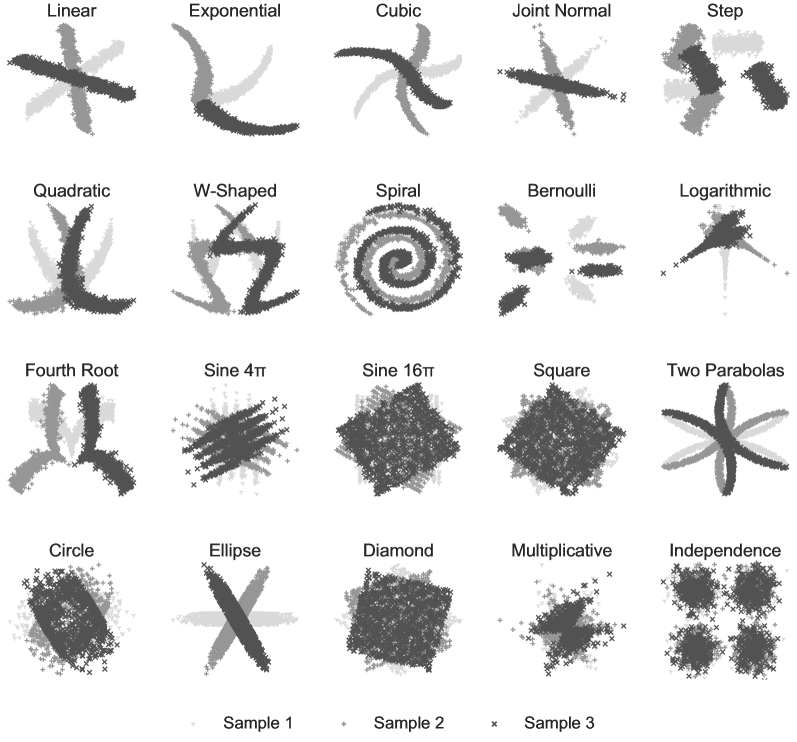
Figure E1: Simulations for power curves. The first dataset (black dots) is 500 samples from each of the 20 two-dimensional, noisy simulation settings from the hyppo package. The two other datasets is the first dataset rotated by 60 degrees clockwise and 60 degrees counter-clockwise. Noise in these simulations are reduced for visualization purposes.

References

- Student [1908] Student. The probable error of a mean. Biometrika, pages 1–25, 1908.
- Hotelling [1992] Harold Hotelling. The generalization of student’s ratio. In Breakthroughs in statistics, pages 54–65. Springer, 1992.
- Fisher [1919] Ronald A Fisher. Xv.—the correlation between relatives on the supposition of mendelian inheritance. Earth and Environmental Science Transactions of the Royal Society of Edinburgh, 52(2):399–433, 1919.
- Bartlett [1947] Maurice S Bartlett. Multivariate analysis. Supplement to the journal of the royal statistical society, 9(2):176–197, 1947.
- Stevens [2002] JP Stevens. Applied multivariate statistics for the social sciences. lawrence erlbaum. Mahwah, NJ, pages 510–1, 2002.
- Warne [2014] Russell Warne. A primer on multivariate analysis of variance (manova) for behavioral scientists. Practical Assessment, Research, and Evaluation, 19(1):17, 2014.
- Székely and Rizzo [2013a] Gábor J Székely and Maria L Rizzo. Energy statistics: A class of statistics based on distances. Journal of statistical planning and inference, 143(8):1249–1272, 2013a.
- Gretton et al. [2012] Arthur Gretton, Karsten M Borgwardt, Malte J Rasch, Bernhard Schölkopf, and Alexander Smola. A kernel two-sample test. Journal of Machine Learning Research, 13(Mar):723–773, 2012.
- Heller et al. [2016] Ruth Heller, Yair Heller, Shachar Kaufman, Barak Brill, and Malka Gorfine. Consistent distribution-free k-sample and independence tests for univariate random variables. The Journal of Machine Learning Research, 17(1):978–1031, 2016.
- Rizzo et al. [2010] Maria L Rizzo, Gábor J Székely, et al. Disco analysis: A nonparametric extension of analysis of variance. The Annals of Applied Statistics, 4(2):1034–1055, 2010.
- Pearson [1895] Karl Pearson. Vii. note on regression and inheritance in the case of two parents. proceedings of the royal society of London, 58(347-352):240–242, 1895.
- Székely et al. [2007] Gábor J Székely, Maria L Rizzo, Nail K Bakirov, et al. Measuring and testing dependence by correlation of distances. The annals of statistics, 35(6):2769–2794, 2007.
- Székely et al. [2009] Gábor J Székely, Maria L Rizzo, et al. Brownian distance covariance. The annals of applied statistics, 3(4):1236–1265, 2009.
- Székely and Rizzo [2013b] Gábor J Székely and Maria L Rizzo. The distance correlation t-test of independence in high dimension. Journal of Multivariate Analysis, 117:193–213, 2013b.
- Lyons et al. [2013] Russell Lyons et al. Distance covariance in metric spaces. The Annals of Probability, 41(5):3284–3305, 2013.
- Gretton et al. [2005] Arthur Gretton, Ralf Herbrich, Alexander Smola, Olivier Bousquet, and Bernhard Schölkopf. Kernel methods for measuring independence. Journal of Machine Learning Research, 6(Dec):2075–2129, 2005.
- Gretton and Györfi [2010] Arthur Gretton and László Györfi. Consistent nonparametric tests of independence. Journal of Machine Learning Research, 11(Apr):1391–1423, 2010.
- Muandet et al. [2017] Krikamol Muandet, Kenji Fukumizu, Bharath Sriperumbudur, Bernhard Schölkopf, et al. Kernel mean embedding of distributions: A review and beyond. Foundations and Trends® in Machine Learning, 10(1-2):1–141, 2017.
- Heller et al. [2012] Ruth Heller, Yair Heller, and Malka Gorfine. A consistent multivariate test of association based on ranks of distances. Biometrika, 100(2):503–510, 2012.
- Shen et al. [2020a] Cencheng Shen, Carey E Priebe, and Joshua T Vogelstein. From distance correlation to multiscale graph correlation. Journal of the American Statistical Association, 115(529):280–291, 2020a.
- Vogelstein et al. [2019] Joshua T Vogelstein, Eric W Bridgeford, Qing Wang, Carey E Priebe, Mauro Maggioni, and Cencheng Shen. Discovering and deciphering relationships across disparate data modalities. eLife, 8:e41690, 2019.
- Panda et al. [2019] Sambit Panda, Satish Palaniappan, Junhao Xiong, Eric W. Bridgeford, Ronak Mehta, Cencheng Shen, and Joshua T. Vogelstein. hyppo: A comprehensive multivariate hypothesis testing python package, 2019.
- Pan et al. [2020] Wenliang Pan, Xueqin Wang, Heping Zhang, Hongtu Zhu, and Jin Zhu. Ball covariance: A generic measure of dependence in banach space. Journal of the American Statistical Association, 115(529):307–317, 2020.
- Shen et al. [2020b] Cencheng Shen, Sambit Panda, and Joshua T. Vogelstein. Learning interpretable characteristic kernels via decision forests, 2020b.
- Winkler et al. [2015] Anderson M Winkler, Matthew A Webster, Diego Vidaurre, Thomas E Nichols, and Stephen M Smith. Multi-level block permutation. Neuroimage, 123:253–268, 2015.
- Sejdinovic et al. [2013] Dino Sejdinovic, Bharath Sriperumbudur, Arthur Gretton, and Kenji Fukumizu. Equivalence of distance-based and rkhs-based statistics in hypothesis testing. The Annals of Statistics, 41(5):2263–2291, 2013.
- Shen and Vogelstein [2021] Cencheng Shen and Joshua T Vogelstein. The exact equivalence of distance and kernel methods in hypothesis testing. AStA Advances in Statistical Analysis, 105(3):385–403, 2021.
- Gorfine et al. [2012] Malka Gorfine, Ruth Heller, and Yair Heller. Comment on detecting novel associations in large data sets. Unpublished (available at http://emotion. technion. ac. il/~ gorfinm/filesscience6. pdf on 11 Nov. 2012), 2012.
- Reshef et al. [2011] David N Reshef, Yakir A Reshef, Hilary K Finucane, Sharon R Grossman, Gilean McVean, Peter J Turnbaugh, Eric S Lander, Michael Mitzenmacher, and Pardis C Sabeti. Detecting novel associations in large data sets. science, 334(6062):1518–1524, 2011.
- Esteban et al. [2019] Oscar Esteban, Christopher J. Markiewicz, Ross W. Blair, Craig A. Moodie, A. Ilkay Isik, Asier Erramuzpe, James D. Kent, Mathias Goncalves, Elizabeth DuPre, Madeleine Snyder, Hiroyuki Oya, Satrajit S. Ghosh, Jessey Wright, Joke Durnez, Russell A. Poldrack, and Krzysztof J. Gorgolewski. fMRIPrep: a robust preprocessing pipeline for functional MRI. Nature Methods, 16(1):111–116, 1 2019. ISSN 1548-7105. 10.1038/s41592-018-0235-4. URL https://www.nature.com/articles/s41592-018-0235-4. Number: 1 Publisher: Nature Publishing Group.
- Abraham et al. [2014] Alexandre Abraham, Fabian Pedregosa, Michael Eickenberg, Philippe Gervais, Andreas Mueller, Jean Kossaifi, Alexandre Gramfort, Bertrand Thirion, and Gael Varoquaux. Machine learning for neuroimaging with scikit-learn. Frontiers in Neuroinformatics, 8, 2014. ISSN 1662-5196. 10.3389/fninf.2014.00014. URL https://www.frontiersin.org/articles/10.3389/fninf.2014.00014/full. Publisher: Frontiers.
- Afshin-Pour et al. [2012] Babak Afshin-Pour, Gholam-Ali Hossein-Zadeh, Stephen C. Strother, and Hamid Soltanian-Zadeh. Enhancing reproducibility of fMRI statistical maps using generalized canonical correlation analysis in NPAIRS framework. NeuroImage, 60(4):1970–1981, 5 2012. ISSN 1095-9572. 10.1016/j.neuroimage.2012.01.137.
- Kettenring [1971] J. R. Kettenring. Canonical Analysis of Several Sets of Variables. Biometrika, 58(3):433–451, 1971. ISSN 0006-3444. 10.2307/2334380. URL https://www.jstor.org/stable/2334380. Publisher: [Oxford University Press, Biometrika Trust].
- Shen et al. [2014] C. Shen, M. Sun, M. Tang, and C. E. Priebe. Generalized canonical correlation analysis for classification. Journal of Multivariate Analysis, 130:310–322, 2014.
- Calhoun et al. [2001] V. D. Calhoun, T. Adali, G. D. Pearlson, and J. J. Pekar. A method for making group inferences from functional MRI data using independent component analysis. Human Brain Mapping, 14(3):140–151, 2001. ISSN 1097-0193. 10.1002/hbm.1048. URL https://onlinelibrary.wiley.com/doi/abs/10.1002/hbm.1048. _eprint: https://onlinelibrary.wiley.com/doi/pdf/10.1002/hbm.1048.
- Bonferroni [1936] C. Bonferroni. Teoria statistica delle classi e calcolo delle probabilita. Pubblicazioni del R Istituto Superiore di Scienze Economiche e Commericiali di Firenze, 8:3–62, 1936. URL https://ci.nii.ac.jp/naid/20001561442.
- Carey [1998] Gregory Carey. Multivariate analysis of variance (manova): I. theory. Retrieved May, 14:2011, 1998.
- Rencher [2002] AC Rencher. Methods of multivariate analysis. DOI, 10(0471271357):66, 2002.
- Bartlett [1939] Maurice S Bartlett. A note on tests of significance in multivariate analysis. In Mathematical Proceedings of the Cambridge Philosophical Society, volume 35, pages 180–185. Cambridge University Press, 1939.
- Rao [1948] C Radhakrishna Rao. Tests of significance in multivariate analysis. Biometrika, 35(1/2):58–79, 1948.
- Garson [2009] G David Garson. Multivariate glm, manova, and mancova. Statnotes: Topics in multivariate analysis, 2009.
- Olson [1976] Chester L Olson. On choosing a test statistic in multivariate analysis of variance. Psychological bulletin, 83(4):579, 1976.
- Olson [1973] Chester Lewellyn Olson. A Monte Carlo investigation of the robustness of multivariate analysis of variance. PhD thesis, Thesis (Ph. D.)–University of Toronto, 1973.
- Micceri [1989] Theodore Micceri. The unicorn, the normal curve, and other improbable creatures. Psychological bulletin, 105(1):156, 1989.
- Stigler [1977] Stephen M Stigler. Do robust estimators work with real data? The Annals of Statistics, pages 1055–1098, 1977.
- Székely et al. [2014] Gábor J Székely, Maria L Rizzo, et al. Partial distance correlation with methods for dissimilarities. The Annals of Statistics, 42(6):2382–2412, 2014.