Downlink Performance of Dense Antenna Deployment: To Distribute or Concentrate?

Abstract

Massive multiple-input multiple-output (massive MIMO) and small cell densification are complementary key 5G enablers. Given a fixed number of the entire base-station antennas per unit area, this paper fairly compares (i) to deploy few base stations (BSs) and concentrate many antennas on each of them, i.e. massive MIMO, and (ii) to deploy more BSs equipped with few antennas, i.e. small cell densification. We observe that small cell densification always outperforms for both signal-to-interference ratio (SIR) coverage and energy efficiency (EE), when each BS serves multiple users via $L$ number of sub-bands (multi-carrier transmission). Moreover, we also observe that larger $L$ increases SIR coverage while decreasing EE, thus urging the necessity of optimal 5G network design. These two observations are based on our novel closed-form SIR coverage probability derivation using stochastic geometry, also validated via numerical simulations.

I Introduction

Performance improvements such as having wider coverage, higher user data rate, higher energy efficiency and lower latency are under an intensive investigation for the design of the fifth generation (5G) and beyond cellular architectures. These improvements are fundamental to achieve the dramatic growth of connected devices and the tremendous amount of data in applications such as voice, videos, and games [1], as well as applications in wireless virtual-reality [2]. Novel innovative network technologies are used to meet the required performances. First, transmission with massive multiple-input multiple-output (MIMO) [3] is considered as a candidate technology for 5G. The key feature of this technology is the use of a large number of antennas at the base station compared to the number of users. The more antennas the base stations are equipped with, the better the performance is in terms of data rate and energy consumption [4]. A second promising technology is small cell networks [5], that consists of a dense number of small cell base stations in a given area. Due to the short distance between the base station (BS) and the user terminals, small cell networks have a low path loss thus yielding a low power consumption which can improve the energy efficiency (EE). For a given total number of BS antennas, interesting strategies in the deployment of these two technologies are either i) low density deployment of base stations with many antennas, i.e, massive MIMO or ii) a higher density deployment of BS s equipped with fewer antennas. Understanding which strategy is preferable is one of the goals of this work.

In fact, many works analyzed the impact of the massive amount of antennas on the EE. In particular, the work in [6] solves the EE maximization problem for a multi-cell multi-user MIMO network and shows that small cells yield higher EE. In [6], the authors give insights on how the number of antennas at the BS must be chosen in order to uniformly cover a given area and attain maximal EE. Altough many works study massive MIMO and small-cell densification, very few have focused on comparing their performance. Our goal is to analyze which one of the two technologies perform better in terms of the coverage probability and energy efficiency.

A comparison has been recently presented in [7]. The massive MIMO and small-cell systems were compared in terms of spectral and energy efficiency bounds. The authors observe via simulations that for the average spectral efficiency, small-cell densification is favourable in crowded areas with moderate to high user density and massive MIMO is preferable in scenarios with low user density. In contrast to the analysis in [7], we derive exact expressions of the coverage probability and EE by assuming other constraints on the model then we compare between massive MIMO and small cell networks in terms of these two metrics. One of the intersting constraint is to assume multi-carrier transmission in which the total bandwidth is divided into $L$ $\geq 1$ sub-bands. Then, instead of studying the downlink performance when each BS serve a single user at each time/frequency, we consider that each BS is scheduled to serve simultaneously multiple users on each sub-band. We also cancel the interference by using zero-forcing (ZF) processing. In addition, instead of introducing massive MIMO and small-cell systems separately, we examine the problem with a single system model by varying the number of BS antennas under the constraint of a fixed total number of BS antennas per unit area. In this work, we derive analytic expressions for the coverage probability and EE using a stochastic geometry approach [8]. The key feature of this approach is that the base station positions are all independent which allows to use tools from stochastic geometry.

The rest of this paper is organized as follows. Section II details our system model of downlink transmission using linear processing ZF under perfect channel state information (CSI) at each base station. General expressions for coverage probability and EE are derived in Section III. In Section IV, numerical results are used to validate the theoretical analysis and make comparisons between massive MIMO and small cell densification for both coverage probability and EE metrics. Finally, the major conclusions and implications are given in Section V.

The following notation is used in this paper. The expectation operation with respect to a random variable and the absolute value are denoted by $\mathbb{E}\{.\}$ and $|.|$, respectively. We denote by $\textbf{I}_{M}$ the $M\times M$ identity matrix, and we use $\mathcal{CN}(0,\bf{\Sigma})$ to denote a circularly symmetric complex Gaussian distribution with zero-mean and covariance matrix $\bf{\Sigma}$. The Gamma function is denoted as $\Gamma(.)$. The bold lower-case letters as h represent vectors, whereas the bold upper-case as H are matrices.

II Network Model

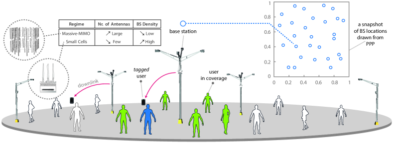
Figure 1: An illustration of the network model.

The cellular network consists of BS s independently distributed according to a homogeneous Poisson point process (PPP) $\Phi$ of intensity $\lambda_{\mathrm{BS}}$ (measured in BS s/$\mathrm{km}^{2}$), and is depicted in Figure 1. Each base station is equipped with an array of $M$ antennas. We consider an independent collection of single antenna mobile users, located according to another independent stationary PPP $\Psi$ with intensity $\lambda_{\mathrm{UE}}$. We assume that each user connects to its closest BS, namely each BS serves the users which are located within its Voronoi cell [9]. In this section, assuming perfect CSI at each BS we study the signal model for downlink system. With this goal in mind, we first consider a typical user, which is connected to a tagged BS ($\mathrm{BS}_{0}$). Since user locations are translation-invariant, we consider that the typical user is always located at the origin. This typical user’s received signal $y$ is then given as

$$y=\underbrace{r_{0}^{-\alpha}\textbf{h}_{0}^{H}\textbf{x}_{0}}_{\mathrm{Desired\ signal}}+\underbrace{\sum\limits_{\begin{subarray}{c}\mathrm{BS}_{i}\in\Phi\backslash\{\mathrm{BS}_{0}\}\end{subarray}}{r_{i}^{-\alpha}\textbf{h}_{i}^{H}\textbf{x}_{i}}}_{\mathrm{Interference}}+n,$$ (1)

where the stochastic vector $\textbf{h}_{i}\in\mathbb{C}^{M}$ denotes the small scale fading between the $i$-th base station to the typical user. It follows a complex generalized Gaussian distribution denoted as $\textbf{h}_{i}\backsim\mathcal{C}\mathcal{N}(0,\textbf{I}_{M})$. The channel is considered to be noisy, with the Gaussian noise $n$ of variance $\frac{K}{P}$ added to the received signal. The variable $r_{i}$ is the distance from the typical user to its closest base station $\mathrm{BS}_{i}$ and $\alpha\geq 2$ is the path-loss exponent. We denote $\mathrm{\textbf{x}_{i}}\in\mathbb{C}^{M}$ an arbitrary symbol transmitted from the $i$-th base station. In addition to the received signal model in (1), we define the signal-to-interference-plus-noise ratio (SINR) of the typical user as

$$\mathrm{SINR}=\dfrac{r_{0}^{-\alpha}\textbf{h}_{0}^{H}\textbf{x}_{0}}{\sum\limits_{\begin{subarray}{c}\mathrm{BS}_{i}\in\Phi\backslash\{\mathrm{BS}_{0}\}\end{subarray}}{r_{i}^{-\alpha}\textbf{h}_{i}^{H}\textbf{x}_{i}+n}}.$$ (2)

We suppose that the BS s must be deployed to match a given finite user density of $\lambda_{\mathrm{UE}}$ $\mathrm{UE}$s/$\mathrm{km}^{2}$, then each base station serves in average $\mathcal{K}=\frac{\lambda_{\mathrm{UE}}}{\lambda_{\mathrm{BS}}}$ users. The total bandwidth $W$ is divided into $L$ $\geq 1$ sub-bands. Therefore, $K=\frac{\mathcal{K}}{L}\leq M$ users are simultaneously served on each sub-band by each base station. We assume that the total number of antennas $\lambda_{\mathrm{BS}}M$ is fixed and should be deployed in a given area. Based on this assumption, for simplicity we set $\lambda_{\mathrm{BS}}M$= $\lambda_{\mathrm{UE}}$, then the number of antennas in each base station is given by $M=\frac{\lambda_{\mathrm{UE}}}{\lambda_{\mathrm{BS}}}$ which is always equal or greater than $K$. We suppose that $P=\mathbb{E}[\mathrm{\textbf{x}}_{i}^{H}\mathrm{\textbf{x}}_{i}]$ is the average transmit power per base station which is given as $\frac{P_{\mathrm{max}}}{\lambda_{\mathrm{BS}}}$, where $P_{\mathrm{max}}$ is the maximum power used when all antennas are concentrated on a single base station. In this scenario, to cancel out the interference while boosting the desired signal power, each BS applies ZF transmission to simultaneously serve $K$ single antennas. Let $s_{i,k}\backsim\mathcal{C}\mathcal{N}(0,1)$ be the message (the symbol) determined for the user $k$ from the $i$-th base station. Then, the $i$-th BS multiplies the data symbol $s_{i,k}$ destined for the $k$-th user by $\mathrm{\textbf{w}_{i,k}}$. Therefore, the linear combination $\mathrm{\textbf{x}_{i}}$ of the symbols transmitted by the $i$-th base station intended for the $K$ users is

$$\textbf{x}_{i}=\sum\limits_{\begin{subarray}{c}k=1\end{subarray}}^{K}{\textbf{w}_{i,k}s_{i,k}},$$ (3)

where $\textbf{w}_{i,k}\in\mathbb{C}^{M\times 1}$ is ZF beamforming vector. Then, the received SINR at the typical user can now be expressed as

$$\mathrm{SINR}=\dfrac{r_{0}^{-\alpha}|\textbf{h}_{0}^{H}\textbf{w}_{0,1}|^{2}}{\sum\limits_{\begin{subarray}{c}\mathrm{BS}_{i}\in\Phi\backslash\{\mathrm{BS}_{0}\}\end{subarray}}{r_{i}^{-\alpha}}\sum\limits_{\begin{subarray}{c}k=1\end{subarray}}^{K}{|\textbf{h}_{i}\textbf{w}_{i,k}|^{2}}+\frac{K}{P}}=\dfrac{r_{0}^{-\alpha}S}{I_{r}+\frac{K}{P}},$$ (4)

where $I_{r}=\sum\limits_{\begin{subarray}{c}\mathrm{BS}_{i}\in\Phi\backslash\{\mathrm{BS}_{0}\}\end{subarray}}{r_{i}^{-\alpha}}g_{i}$ with $g_{i}=\sum\limits_{\begin{subarray}{c}k=1\end{subarray}}^{K}{|\textbf{h}_{i}\textbf{w}_{i,k}|^{2}}$ denotes the interference channel power and $S=|\textbf{h}_{0}^{H}\textbf{w}_{0,1}|^{2}$ is the desired channel power. Now, we introduce the metrics we will investigate in the next sections.

Definition 1 (Coverage Probability).

The coverage probability of a typical user is the the probability that the SINR received by the user is larger than a predefined threshold $T$ such as

$$\mathbb{P}_{\mathrm{cov}}(T)=\mathbb{P}(\mathrm{SINR}>T).$$ (5)

Definition 2 (Energy Efficiency).

The EE is defined as

$$\footnotesize\mathrm{EE}=\dfrac{\mathrm{ASE}}{\mathrm{AEC}}=\dfrac{\mathrm{Area\ Spectral\ Efficiency}\;\mathrm{[bit/symbol/km^{2}]}}{\mathrm{Average\ Energy\ Consumption}\;\mathrm{[Joule/symbol/km^{2}]}},$$ (6)

where the area spectral efficiency (ASE) is expressed as

$$\mathrm{ASE}=\lambda_{\mathrm{BS}}K\mathbb{E}[R],$$ (7)

in which $\lambda_{\mathrm{BS}}$ represents BS density, $K$ is the number of users that are served by the BSs and $\mathbb{E}[R]$ is the average data rate of users. Moreover, average energy consumption (AEC) is defined as similar to [10], that is

$$\mathrm{AEC}=\left(\dfrac{P}{\eta}+MP_{\mathrm{c}}+K^{3}P_{\mathrm{pre}}+P_{\mathrm{0}}\right),$$ (8)

where $\eta$ denotes the power amplifier efficiency, $P_{c}$ is the circuit power per antenna, which indicates the energy consumption of the corresponding RF chains. The term $K^{3}P_{\mathrm{pre}}$ accounts for the energy consumption for precoding which is related to the number of users served simultaneously by each base station. The term $P_{0}$ is the non-transmission power, which accounts for the energy consumption of baseband processing.

Remark 1.

The goal in EE is to maximize the performance while minimizing the energy consumption which are two conflicting operations in 5G.

III Performance Analysis

In this section we give the analytical expression of the coverage probability on a typical mobile user. Afterwards, we shall give the expression of the EE. We start by stating the following Lemma that shall be used to derive our results.

Lemma 1 ([9]).

The probability density function (PDF) of a typical user’s association distance $r_{0}$ is

$$f_{r_{0}}(r)=\frac{dF_{r_{0}}(r)}{dr}=e^{-\lambda_{\mathrm{BS}}\pi r^{2}}2\pi\lambda_{\mathrm{BS}}r.$$ (9)

Proof.

Each user is connected to its closest base station, then all the interfering base stations are farther than a distance $r$. Since the Poisson distribution helps in describing the chances of occurrence of a number of events in a given space, then the probability that no base station is closer than a distance $r$ within an area $\pi r^{2}$, is $e^{-\lambda_{\mathrm{BS}}\pi r^{2}}$, expressed as

$$\mathbb{P}(r_{0}>r)=F_{r_{0}}(r)=\mathbb{P}[\mathrm{No\ BS}\ \mathrm{within}\ \pi r^{2}]=e^{-\lambda_{\mathrm{BS}}\pi r^{2}}$$ (10)

Therefore, the PDF results from the derivative of the cumulative distribution function $F_{r}(R)$. ∎

III-A Coverage Probability

Before deriving the expression of the coverage probability, we first derive the Laplace transform of both interference and desired signal. The desired channel power $S$ is distributed as $\Gamma(M-K+1,1)$ [11]. For the interfering signal, as $\textbf{w}_{i,k}$ is a unit-norm vector and independent of $\textbf{h}_{i}$, then $|\textbf{h}_{i}\textbf{w}_{i,k}|^{2}$ is a squared-norm complex Gaussian, which is exponential distributed. For tractability we neglect the correlation between $\textbf{w}_{i,k}$ for different $k$, then the channel gain $g_{i}$ is the sum of $K$ independent exponential distributed random variables which follows $\Gamma(K,1)$.

Lemma 2 (Laplace Transform of Interference).

The Laplace transform of interference $\mathcal{L}_{I_{r}}(s)$=$\mathbb{E}[e^{-sI_{r}}]$ is

$$\mathcal{L}_{I_{r}}(s)=\exp\left[-\pi\lambda_{\mathrm{BS}}r_{0}^{2}\left(-1+\mathrm{{}_{2}F_{1}}\left(K,\dfrac{-2}{\alpha};\dfrac{-2}{\alpha}+1;-sr_{0}^{-\alpha}\right)\right)\right],$$ (11)

where ${}_{2}\mathrm{F}_{1}$ is the Gauss-Hypergeometric function.

Proof.

See Appendix A. ∎

Lemma 3 (Laplace Transform of the Desired Signal).

The Laplace transform of the desired signal $\mathcal{L}_{S}(s)=\mathbb{E}[e^{-sS}]$ is

$$\mathcal{L}_{S}(s)=\left(\dfrac{1}{1+s}\right)^{M-K+1}.$$ (12)

Proof.

See Appendix B. ∎

Combining the previous results given in Lemmas 1, 2 and 3 with the proof techniques proposed in [12], an expression for the coverage probability can be derived and it is given in the following theorem.

Theorem 1 (Coverage Probability in Downlink).

The coverage probability at a typical mobile user in the general cellular network model described above is

$$\begin{split}\mathbb{P}_{\mathrm{cov}}(T)=\displaystyle{\int_{r_{0}>0}}\displaystyle{\int_{-\infty}^{\infty}}\mathcal{L}_{I_{r_{0}}}(&i2\pi r^{\alpha}_{0}Ts)\exp\left(-\dfrac{i2\pi r_{0}^{\alpha}TK}{P}s\right)\\ &\times\dfrac{\mathcal{L}_{S}(-i2\pi s)-1}{i2\pi s}f_{r_{0}}(r_{0})\mathrm{d}s\mathrm{d}r_{0},\end{split}$$ (13)

where $f_{r_{0}}(r_{0})$ is the PDF of the distance between the typical user and the tagged base station ($\mathrm{BS}_{0}$), $\mathcal{L}_{I_{r_{0}}}(.)$ is the Laplace transform of the interference and $\mathcal{L}_{S}(.)$ is the Laplace transform of the desired signal (Lemmas 1, 2 and 3 respectively).

Proof.

See Appendix C. ∎

III-B Energy Efficiency

$$\small\mathrm{EE}=\dfrac{\lambda_{\mathrm{BS}}K\displaystyle{\int_{r_{0}>0}}\displaystyle{\int_{-\infty}^{\infty}}\mathcal{L}_{I_{r_{0}}}(i2\pi r^{\alpha}_{0}Ts)\exp\left(-\dfrac{i2\pi r_{0}^{\alpha}TK}{P}s\right)\times\dfrac{\mathcal{L}_{S}(-i2\pi s)-1}{i2\pi s}f_{r_{0}}(r_{0})\mathrm{d}s\mathrm{d}r_{0}\log(1+T)}{\left(\dfrac{P}{\eta}+MP_{\mathrm{c}}+K^{3}P_{\mathrm{pre}}+P_{\mathrm{0}}\right)}$$ (14)

 

To facilitate the analysis of the EE, we consider fixed modulation and coding schemes for each user by considering a fixed $\mathrm{SINR}$ threshold $T$ as in [13], providing the average rate $\mathbb{E}[R]$ as a function of downlink coverage probability as

$$\begin{split}\mathbb{E}[R]=&\log(1+T)\mathbb{P}_{\mathrm{cov}}(T)\\ =&\log(1+T)\displaystyle{\int_{r_{0}>0}}\displaystyle{\int_{-\infty}^{\infty}}\mathcal{L}_{I_{r_{0}}}(i2\pi r^{\alpha}_{0}Ts)\times\\ &\exp\left(-\dfrac{i2\pi r_{0}^{\alpha}TK}{P}s\right)\dfrac{\mathcal{L}_{S}(-i2\pi s)-1}{i2\pi s}f_{r_{0}}(r_{0})\mathrm{d}s\mathrm{d}r_{0},\end{split}$$ (15)

By plugging the average rate expression into (7), we obtain the ASE. Then, the expressions of EE can be readily obtained and its final expression is given in (14) on the top of this page.

IV Numerical Results

Table I: Default Simulation Parameters.

System Parameter	Symbol	Value
Power amplifier	$\eta$	$0.318$
Circuit power per antenna	$P_{\mathrm{c}}$	$14.8$ $\mathrm{W}$
Energy consumption for precoding	$P_{\mathrm{pre}}$	$1.74$ $\mathrm{W}$
Nr. of Sub-bands	$L$	$1$
Target $\mathrm{SINR}$	$T$	1 $\mathrm{dBm}$
Non-transmission power	$P_{0}$	$65.8$ $\mathrm{W}$
Maximum average power per BS	$P_{\mathrm{max}}$	$40$ $\mathrm{dBm}$
Users density	$\lambda_{\mathrm{UE}}$	$32$ per $\mathrm{km}^{2}$
BS density	$\lambda_{\mathrm{BS}}$	$4$
Path-loss exponent	$\alpha$	$4$

(a)

(b)

(c)

(d)

Figure 2: Evolution of coverage probability with respect to the a) the target $\mathrm{SINR}$. b) the BS density in BS/$\mathrm{km}^{2}$, and c) number of sub-bands $L$. The subfigure d) shows the evolution of EE with respect to the BS density in BS/$\mathrm{km}^{2}$.

In this section, we conduct Monte-Carlo simulations to validate the analytical expressions of coverage probability and EE of our multi-user MIMO system. The default parameter setting is given in Table I and shall be used unless otherwise stated.

Figure 2(a) illustrates the coverage probability expression provided in Theorem 1 as a function of target $\mathrm{SINR}$ for three different path-loss values: $\alpha\in\{3,4,5\}$. The curves reveal that the coverage probability obtained by simulation behaves exactly as the analytical results which confirm the accuracy of our theoretical expressions. Also, increasing $\alpha$ increases the coverage probability because the interference power decreases faster as a function of $\alpha$ than the power signal [14].

Figure 2(b) shows the coverage probability as a function of BS density. Several important observations can be made from the results of this figure. First, for any given $L$, the coverage probability can be greatly improved by increasing the BS density, meaning that distributed network densification is preferable over massive MIMO. Second, we note that the coverage probability increases as $L$ increases, thus showing the importance of multi-carrier transmissions. However, it is shown that for large $L$, both massive MIMO and small cells provide the same coverage which is confirmed according to Figure 2(c). This phenomenon occurs since the number of users $K$ served by each BS decreases and become very small compared to the number of its own antennas $M$.

Figure 2(d) shows the impact of varying $\lambda_{\mathrm{BS}}$ on the EE. The curves show that for any given $L$, the EE can also be improved by increasing the BS density, meaning that small cells is also preferable over massive MIMO. In contrast with the coverage probability, we can observe that in small cells scenario, decreasing the number of sub-bands $L$ increases the EE but in massive MIMO scenario, large number of sub-bands provides the highest EE. Finally, we notice also that both massive MIMO and small cells provide the same performance gain when $L$ becomes very large which means that the EE increase when the number of users served by the base station approach the number of its base station antennas $M$. All these observations show that the coverage and EE are conflicting such that improvements in one objective lead to degradation in the other objective for a fixed number of sub-bands $L$.

V Conclusions

Our proposed model was based on stochastic geometry, where the BS and user locations were distributed according to PPP. Using tools from stochastic geometry, we derived the coverage probability and EE expressions for downlink scenario. The coverage probability expression was validated via Monte-Carlo simulations. The comparison showed that for any given sub-band $L$, small cell densification is preferable over massive MIMO if both coverage probability and EE should be increased. However, increasing $L$ improves the coverage probability but decreases the EE which shows that the two metrics are conflicting. An interesting future work is therefore to introduce a multi-objective optimization framework and find (possibly) optimal number of sub-bands and BS density that maximize the coverage probability and EE jointly for the uplink and downlink scenarios. Future work will also look at multiple antenna terminals which is still an open topic.

Appendix A Proof of Lemma 2

Let $f(g)$ and $f(S)$ denote the PDF of $g_{i}=\sum\limits_{\begin{subarray}{c}k=1\end{subarray}}^{K}{|\mathrm{\textbf{h}}_{i}\mathrm{\textbf{w}}_{i,k}|^{2}}$ and $S=|\mathrm{\textbf{h}}_{0}^{H}\mathrm{\textbf{w}}_{0,1}|^{2}$ respectively. The Laplace transform of the interference is $\mathcal{L}_{I_{r}}(s)=\mathbb{E}[e^{-sI_{r}}]$, where the average is taken over both the spatial PPP and the interference distribution is expressed as follows:

$$\begin{split}\mathcal{L}_{I_{r}}(s)&=\mathbb{E}_{\Phi,\{g_{i}\}}\left[\exp\left(-s\sum\limits_{\begin{subarray}{c}\mathrm{BS}_{i}\in\Phi\backslash\{\mathrm{BS}_{0}\}\end{subarray}}{r_{i}^{-\alpha}g_{i}}\right)\right],\\ &=\mathbb{E}_{\Phi,\{g_{i}\}}\left[\underset{\mathrm{BS}_{i}\in\Phi\setminus\{\mathrm{BS}_{0}\}}{\prod}\left[\exp(-sg_{i}r_{i}^{-\alpha})\right]\right],\\ &\overset{(a)}{=}\mathbb{E}_{\Phi}\left[\underset{\mathrm{BS}_{i}\in\Phi\setminus\{\mathrm{BS}_{0}\}}{\prod}\mathbb{E}_{g_{i}}\left[\exp(-sg_{i}r_{i}^{-\alpha})\right]\right],\\ &\overset{(b)}{=}\mathbb{E}_{\Phi}\left[\underset{\mathrm{BS}_{i}\in\Phi\setminus\{\mathrm{BS}_{0}\}}{\prod}\frac{1}{\Gamma(K)}\displaystyle{\int_{0}^{\infty}}e^{-g_{i}(sr_{i}^{-\alpha}+1)}g_{i}^{K-1}\mathrm{d}g_{i}\right],\\ &\overset{(d)}{=}\mathbb{E}_{\Phi}\left[\underset{\mathrm{BS}_{i}\in\Phi\setminus\{\mathrm{BS}_{0}\}}{\prod}\frac{1}{(1+sr_{i}^{-\alpha})^{K}}\right],\\ &\overset{}{=}\exp\left(-2\pi\lambda_{\mathrm{BS}}\displaystyle{\int_{r_{0}}^{\infty}}\left(1-\frac{1}{(1+sv^{-\alpha})^{K}}\right)v\mathrm{d}v\right)\end{split}$$ (16)

where the step (a) follows from the i.i.d distribution of $g_{i}$ and further independence from the point process $\Phi$. The step (b) follows from the PDF of $g_{i}$ $\backsim$ $\Gamma(K,1)$ given as

$$f(g)=\frac{1}{\Gamma(K)}g^{K-1}e^{-g_{i}}.$$ (17)

Moreover, the step (c) follows from the computation of the integral by the means of integration by parts. The last step follows from the probability generating functional of the PPP with intensity $\lambda$ [9], which states that for some function $f(x)$ we have

$$\mathbb{E}\left[\underset{\mathrm{BS}_{i}\in\Phi\setminus\{BS_{0}\}}{\prod}f(x)\right]=\exp\left(-\lambda\displaystyle{\int_{\mathbb{R}^{2}}}(1-f(x)\mathrm{d}x)\right).$$ (18)

The inside integral can be evaluated by using the change of variables $v^{-\alpha}\rightarrow y$ and we obtain the result. ∎

Appendix B Proof of Lemma 3

The Laplace transform of the desired signal is $\mathcal{L}_{S}(s)=\mathbb{E}[e^{-sS}]$, where the average is taken over the desired signal distribution expressed as follows:

$$\begin{split}\mathcal{L}_{S}(s)&=\mathbb{E}_{S}[e^{-sS}]\\ &\overset{}{=}\frac{1}{\Gamma(M-K+1)}\displaystyle{\int_{0}^{\infty}}S^{M-K}e^{-S(1+s)}\mathrm{d}S,\\ &\overset{a}{=}\left(\frac{1}{1+s}\right)^{M-K+1},\end{split}$$ (19)

where the first step follows from the PDF of the desired signal

$$f(S)=\frac{1}{\Gamma(M-K+1)}S^{M-K}e^{-S}\mathrm{d}S.$$ (20)

The step (a) follows from the computation of the integral by the means of integration by parts. ∎

Appendix C Proof of Theorem 1

The first part of the proof follows by conditioning on the nearest BS being at a distance $r_{0}$ from the typical user. Then, the probability of coverage is

$$\mathbb{P}_{\mathrm{cov}}(T,\lambda_{\mathrm{BS}},\alpha)=\displaystyle{\int_{r_{0}>0}}e^{-\pi\lambda_{\mathrm{BS}}r_{0}^{2}}\ \mathbb{P}(\frac{r_{0}^{-\alpha}S}{I_{r}+\frac{K}{P}}>T)\ 2\pi\lambda_{\mathrm{BS}}r_{0}\mathrm{d}r_{0}.$$ (21)

To evaluate $\mathbb{P}(\frac{r_{0}^{-\alpha}S}{I_{r}+\frac{K}{P}}>T)$, we use the proof techniques proposed in [14] and [12]. Some assumptions are required for this computation:

• The desired signal $S$ admits a square integrable density.

• Either the interference $I_{r}$ or the noise admits a density which is square integrable.

The interference and the noise are independent, then the second assumption imply that $I_{r}+\frac{K}{P}$ admits a PDF $f_{I_{r}+\frac{K}{P}}(y)$ that is square integrable. Therefore, the coverage probability is expressed as follows:

$$\begin{split}\mathbb{P}\left(\mathrm{SINR}>T\right)&=\mathbb{P}\left(\dfrac{r^{-\alpha}S}{I_{r}+\frac{K}{P}}>T\right),\\ &=\mathbb{P}\left(I_{r}+\frac{K}{P}<(Tr_{0}^{\alpha})^{-1}S\right),\\ &=\mathbb{E}_{S}\left\{\mathbb{P}\left(I_{r}+\frac{K}{P}<(Tr_{0}^{\alpha})^{-1}S\right)\right\},\\ &\overset{(a)}{=}\mathbb{E}_{S}\left\{\displaystyle{\int_{0}^{S(Tr_{0}^{\alpha})^{-1}}}f_{I_{r}+\frac{K}{P}}(y)\mathrm{d}y\right\},\\ &=\mathbb{E}_{S}\left\{\displaystyle{\int_{-\infty}^{+\infty}}f_{I_{r}+\frac{K}{P}}(y)\textbf{1}_{\left[0\leq y\leq S(Tr_{0}^{-\alpha})^{-1}\right]}\mathrm{d}y\right\}.\end{split}$$ (22)

where the step (a) above follows from the definition

$$\mathbb{P}(a\leq X\leq b)=\displaystyle{\int_{a}^{b}f(x)\mathrm{d}x},$$ (23)

where $f$ is the density function of the variable $X$. Using the Plancheral-Parseval theorem [15], we obtain

$$=\mathbb{E}_{S}\left\{\displaystyle{\int_{-\infty}^{+\infty}}e^{-2\pi isI_{r}}\ \exp\left(-2i\pi\frac{K}{P}s\right)\dfrac{e^{2i\pi ys(Tr_{0}^{\alpha})^{-1}}-e^{2i\pi ys\times 0}}{2i\pi s}\mathrm{d}s\right\},$$

$$=\mathbb{E}_{S}\left\{\displaystyle{\int_{-\infty}^{+\infty}}\mathcal{L}_{I_{r}}(-2i\pi Tr_{0}^{\alpha}s)\ \exp\left(-2i\pi\frac{K}{P}Tr_{0}^{\alpha}s\right)\frac{e^{2i\pi ys}-1}{2i\pi s}\mathrm{d}s\right\}.$$

Using Fubini’s theorem [16], and moving the expectation inside

$$=\displaystyle{\int_{-\infty}^{+\infty}}\mathbb{E}_{S}\left\{\mathcal{L}_{I_{r}}(-2i\pi Tr_{0}^{\alpha}s)\ \exp\left(-2i\pi Tr_{0}^{\alpha}\frac{K}{P}s\right)\dfrac{e^{2i\pi ys}-1}{2i\pi s}\right\}\mathrm{d}s,$$

$$=\displaystyle{\int_{-\infty}^{+\infty}}\mathcal{L}_{I_{r}}(-2i\pi Tr_{0}^{\alpha}s)\ \exp\left(-2i\pi Tr_{0}^{\alpha}\frac{K}{P}s\right)\dfrac{\mathcal{L}_{S}(e^{2i\pi ys})-1}{2i\pi s}\mathrm{d}s.$$

Combining the last expression and (21) gives the result stated in Theorem 1. ∎

References

- [1] Cisco, “Cisco visual networking index: Global mobile data traffic forecast update 2016–2021,” White Paper, 2017. [Online]. Available: https://goo.gl/HdxsI0
- [2] E. Baştuğ, M. Bennis, M. Médard, and M. Debbah, “Towards interconnected virtual reality: Opportunities, challenges and enablers,” IEEE Communications Magazine, arXiv preprint arXiv: 1611.05356, 2017.
- [3] J. Hoydis, S. Ten Brink, and M. Debbah, “Massive MIMO in the UL/DL of cellular networks: How many antennas do we need?” IEEE Journal on selected Areas in Communications, vol. 31, no. 2, pp. 160–171, 2013.
- [4] K.-K. Wong, R. D. Murch, and K. B. Letaief, “Performance enhancement of multiuser MIMO wireless communication systems,” IEEE Transactions on Communications, vol. 50, no. 12, pp. 1960–1970, December 2002.
- [5] J. Hoydis, M. Kobayashi, and M. Debbah, “Green small-cell networks,” IEEE Vehicular Technology Magazine, vol. 6, no. 1, pp. 37–43, March 2011.
- [6] E. Björnson, L. Sanguinetti, J. Hoydis, and M. Debbah, “Optimal design of energy-efficient multi-user MIMO systems: Is massive MIMO the answer?” IEEE Transactions on Wireless Communications, vol. 14, no. 6, pp. 3059–3075, March 2015.
- [7] H. D. Nguyen and S. Sun, “Massive MIMO versus small-cell systems: spectral and energy efficiency comparison,” in IEEE International Conference on Communications (ICC). IEEE, 2016, pp. 1–6.
- [8] F. Baccelli, B. Błaszczyszyn et al., “Stochastic geometry and wireless networks: Volume ii applications,” Foundations and Trends® in Networking, vol. 4, no. 1–2, pp. 1–312, 2010.
- [9] M. Haenggi, Stochastic geometry for wireless networks. Cambridge University Press, October 2012.
- [10] Q. Zhang, C. Yang, H. Haas, and J. S. Thompson, “Energy efficient downlink cooperative transmission with BS and antenna switching off,” IEEE Transactions on Wireless Communications, vol. 13, no. 9, pp. 5183–5195, 2014.
- [11] H. S. Dhillon, M. Kountouris, and J. G. Andrews, “Downlink MIMO Hetnets: Modeling, ordering results and performance analysis,” IEEE Transactions on Wireless Communications, vol. 12, no. 10, pp. 5208–5222, August 2013.
- [12] F. Baccelli, B. Blaszczyszyn, and P. Muhlethaler, “Stochastic analysis of spatial and opportunistic ALOHA,” IEEE Journal on Selected Areas in Communications, vol. 27, no. 7, pp. 1105–1119, September 2009.
- [13] J. Park and P. Popovski, “Coverage and rate of downlink sequence transmissions with reliability guarantees,” arXiv preprint: 1704.05296, 2017.
- [14] J. G. Andrews, F. Baccelli, and R. K. Ganti, “A tractable approach to coverage and rate in cellular networks,” IEEE Trans. Commun., vol. 59, no. 11, pp. 3122–3134, November 2011.
- [15] P. Brémaud, Mathematical principles of signal processing: Fourier and wavelet analysis. Springer Science & Business Media, 2013.
- [16] J. A. León, “Fubini theorem for anticipating stochastic integrals in Hilbert space,” Applied Mathematics and Optimization, vol. 27, no. 3, pp. 313–327, 1993.