Noise level forecasts at 8-20MHz and their use for morphological studies of ionospheric absorption variations at EKB ISTP SB RAS radar

Abstract

In this paper, a method is described for using 8-20MHz noise absorption effect for realtime detecting radiowave absorption periods. The method is based on two empirical autoregression models of noise dynamics. The first (rough) prediction model is based on radar measurements of daily minimal noise dynamics averaged over 28-days with specially calculated weight coefficients. The second (fine) prediction model uses real-time scaling of rough model. The scaling is based on the comparison of this model with the experimental noise observations during previous 5 days. The models are based on the whole EKB ISTP SB RAS radar dataset (2013-2018). The rough model allows one to estimate the boundary beyond which the noise variations can be associated with absorption periods with a high degree of certainty. A joint analysis of simultaneous data on neighboring radar beams and at several frequencies reduces the detection errors, and allows to identify absorption events with a higher degree of confidence. Use of fine model allows to estimate absorption. The technique is validated by frequency dependence of absorption during two-frequency measurements. The found frequency dependence has an average exponent of the order of -1.5, which is in good agreement with the literature data and the data obtained earlier in analysis of solar X-ray flares. The use of the detection technique at EKB radar shows that most probable absorption over absorption events is about -0.65dB. Analysis of absorption of different amplitudes shows that low-intensity absorption events (0..-1.3dB) have slight local time dependence and mostly observed at north directions. For the storng absorption events (stronger than -1.3dB) the local time dynamics correlates well with noise level dynamics, and usually fills the whole radar field-of-view.

1 Introduction

The use of 8-20MHz radio noise, measured by short-wave radars for the diagnosis of the lower part of the ionosphere, is an intensively developed method [1, 2, 3, 4, 5]. The physical processes that cause this effect [4] are close to the physical processes that cause the absorption of the signals scattered from the earth’s surface (ground scatter, GS) [6, 7], so GS signals and noise level both can be used to study the absorption of radiwaves [5]. The first observations of the absorption of 8-20 MHz radio noise during X-ray solar flares at mid-latitude radars [1] showed the efficiency of this method. Subsequent statistical analysis according to the data of world-wide radar network showed usefulness of this method in the lit time: it allows approve the main influence of the ionosphere near the radar to the absorption; it allows demonstrate the contributions of D- and E-layers to the absorption; it allows estimate the frequency dependence of absorption; it allows localize the region in which the absorption measured [4]. Studies of absorption associated with the corpuscular solar radiation allow demonstrate a good agreement between radio noise 8-20MHz absorption and standard observations by riometers [2, 3], allowing to prove the correctness of the technique in these cases too.

Therefore, an important practical issue is creation an automatic detector system for detecting the periods of radio signal absorption from the 8-20MHz noise data. Similar systems are usually based on riometric noise prediction model, allowing to make an accurate forecast of the noise level for a significant period of time ahead of the observations, exceeding the duration of the expected effects. The prediction time and accuracy of the forecast determines the accuracy of absorption detection technique. It should be noted that the periods of radio noise absorption can be short-term (up to several hours)[1, 4] or long-term [2, 3]. Most of the recent papers is currently devoted to case studying during selected events [1, 2, 3, 4], and a complete analysis of all cases of absorption using coherent radars has not yet been carried out.

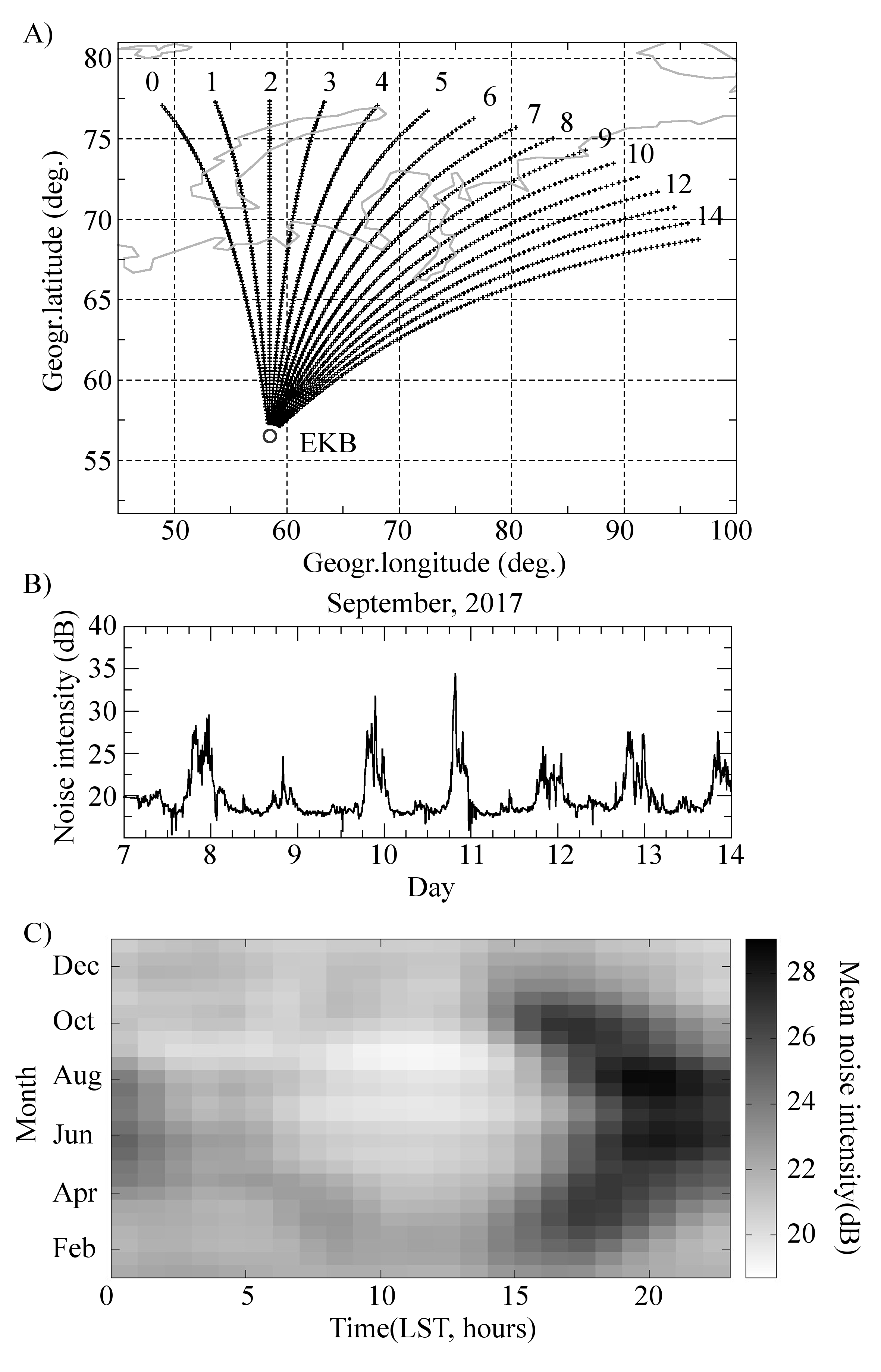
Figure 1: A) Geographical location of the EKB ISTP SB RAS radar and its field of view. The lines correspond to the trajectories (beams) of the radiosignal propagation, the numbers mark the beam numbers. B) An example of noise level variations during September 7-13, 2017; C) The average noise level on beam 2 as a function of the month number and local solar time(LST).

The EKB ISTP SB RAS radar is a mid-latitude decameter radar of CUTLASS kind [8] developed at the University of Leicester, similar in design and software to SuperDARN (Super Dual Auroral Radar Network) [9, 10, 11] radars. The radar was bought under the financial support of SB RAS, and was installed together with the IGF UrB RAS near Ekaterinburg, in Arti observatory, IGF UrB RAS (56.5N, 58.5E). The radar field of view is about 1 million square kilometers and is shown in Fig.1A. In regular mode, the radar operates in 16 discrete directions (beams) with 1-2 minute temporal resolution, with 45 km spatial resolution, and at the operating frequencies 8-20 MHz. The radar transmits sequences of short sounding pulses and processes the received signals, scattered from surface and ionospheric irregularities. This information is used to investigate an ionospheric characteristics within the radar field-of-view. Between the soundings, the radar measures the noise level near the sounding frequency to select the frequency at which the background noise level is minimal. An example of the noise dynamics, measured at a single beam and a single frequency is shown in Fig.1B. The radar operates simultaneously in two frequency channels, which makes it possible to measure the properties of the scattered signal and the noise level in two frequencies simultaneously and independently.

It was shown that the analysis of the minimal noise level allows using the radar as a mid-latitude riometer[1, 2, 3, 4]. An essential issue associated with this use is the reliable prediction of noise dynamics to calculate the amplitude of noise attenuations considered as absorption.

The short-wave radio noise is produced by a superposition of signals from various sources (anthropogenic, space and atmospheric), and each of them has its own seasonal, daily and geographical dependency [12]. The mechanism of long-range multihop radiwave propagation at 8-20 MHz makes the prediction of the noise level a difficult task. The radio noise observed at SuperDARN and similar radars has significant daily and seasonal dependencies [13, fig.6] and currently its reference models suitable for reliable forecast are apparently absent. The average daily-seasonal noise level dynamics at EKB ISTP SB RAS radar is shown in Fig.1C for the beam 2, directed to the North. It can be seen from the figure that the mean daily noise dynamics significantly depends on the season and the noise level has a pronounced maximum during sunset solar terminator and a minimum in the local noon. This effect is similar to the effect observed earlier by the Canadian SAS SuperDARN radar [13, fig.6]. Therefore, the use of simple stationary models for noise prediction is problematic, and the predictive model should either include the physical mechanisms of the noise formation or use the noise historical observations.

2 Noise prediction model

The traditional approach used in riometric observations is to use the simplest mean daily noise model, averaged over previous 30 days [14], or use database of quiet days to select the quiet day curve [15]. We will use the first one as the simplest. Its use can be justified in cases where the effects of the propagation of radio waves can be neglected (which is acceptable for the frequencies 30-40 MHz used by riometers). In spite the possibility and effectiveness of using such models for noise prediction in some cases at SuperDARN radar [2], their validity and accuracy for all cases is not obvious. Due to the fact that the noise level on radars is affected not only by the absorption itself, but also by the ionospheric F-layer dynamics affecting the propagation trajectory of the noise [4], the use of the mean daily noise model is not entirely justified.

In this paper, the problem of predicting 8-20 MHz radio noise level from experimental data is considered as a combination of two problems - making a rough prediction model of the minimal noise level (i.e. the long-term prediction of dynamics of minimal noise associated with regular processes both in the ionosphere and in the noise sources) and making a technique for forecasting mean noise level in real-time by correcting this model. The accuracy of the forecast will depend on a combination of the accuracy of these two techniques. In the both cases, we used an autoregression analysis to build the optimal prediction algorithm.

To build the first (rough) prediction model a regression coefficients were found (based on a large observational base of EKB radar measurements during 2013-2016), that optimally predict the minimal noise level based on the measurements of the minimal noise in the same local time over previous days. The prediction model is built as an autoregression with the calculated coefficients. The minimal noise is used because the radar often detects interference from a nearby ionosonde and other anthropogenic sources, and the use of minimal noise should compensate this interference.

To build the second (fine) prediction model, we calculated coefficients allowed us to scale (calibrate) the rough model of minimal noise to optimally fit the experimental data 12 hours ahead. The coefficients were obtained using the entire history over the several previous days and using the rough model of minimal noise for all these moments. The analysis of the whole EKB dataset make it possible to determine the optimal duration of the calibration period, and the values of the optimal weighting coefficients for the calibration.

Let us consider these two models in details.

Rough prediction model of the minimal noise level

To build the model of the diurnal dynamics of the minimal noise, the approximate 24-hour periodicity of the noise level is taken into account (shown in Fig.1B). In spite of a strong variations of noise level in the experimental data, the amplitude and shape of the mean diurnal variation of noise level looks changing slowly. Therefore, as a model of the diurnal noise level dynamics, we use an autoregression dependence over measurements in the previous days, at the same time. As mentioned above, a close approach is used for analysis of a riometric data by using 30-day history to predict mean daily noise dynamics [14].

To exclude the interference associated with the operation of the nearby ionosonde, as well as with iregular nearby anthropogenic sources, we use the minimal noise levels determined over the 5-minute period (it corresponds to approximately three scans over the entire radar field-of-view) as inputs. The minimal noise level $f_{m,min}(t)$ for 24 hours ahead is predicted as the autoregression:

$$\begin{array}[]{l}f_{m,min}(t;f_{sound},B_{m})=\sum_{n=1}^{\infty}R_{n}f_{e,min}(t-n\triangle T;f_{sound},B_{m})\\ f_{e,min}(\tau;f_{sound},B_{m})=\left.Min\left(f_{e}(t^{\prime};f_{sound},B_{m})\right)\right|{}_{t^{\prime}=\tau-dT/2}^{\tau+dT/2}\end{array}$$ (1)

here $dT$ is the time interval of noise minimization (5 minutes),$\triangle T$ is the main period of the diurnal variations (24 hours), $f_{e}(t^{\prime})$ is the experimentally measured noise level (dB) at the moment $t^{\prime}$; $f_{sound}$ is approximate value of sounding frequency (with accuracy $\pm 500kHz$), $B_{m}$ is the radar beam number, $f_{e,min}(\tau;f_{0},B_{m})$ is minimal noise level over period $[\tau-dT/2,\tau+dT/2]$.

To determine and verify the regression coefficients $R_{n}$, the whole available EKB radar dataset is divided into two periods - the training dataset 2013-2016 and the test dataset 2017-2018. The optimal regression coefficients $R_{n}$, which provide the most accurate prediction of the minimal noise level, are calculated over the training dataset 2013-2016 as a result of the following minimization:

$$\varOmega_{1}(f_{0},B_{m})=\int\left(f_{m,min}(t;f_{0},B_{m})-f_{e,min}(t;f_{0},B_{m})\right)^{2}dt=min$$ (2)

To speed up the calculations, the regression coefficients $R_{n}$ are estimated over the sequences with 15 minute temporal resolution, and only over the sequences lasting at least 40 days (sufficient for determining 40 daily regression coefficients $R_{n}$). The regression is carried out separately and independently for each beam and in each sounding frequency range. After this the obtained regression coefficients for all beams and all frequencies are averaged to obtain the average regression coefficients $R_{n}$ and to estimate the variance of each coefficient. To improve the accuracy for calculation of Eq.(2) only the data from the beams and the frequencies were used with number of available measurements exceeded 1000. The obtained average regression coefficients $R_{n}$ and their root mean square (RMS) error are shown in Fig.2A by thick and thin black lines correspondingly.

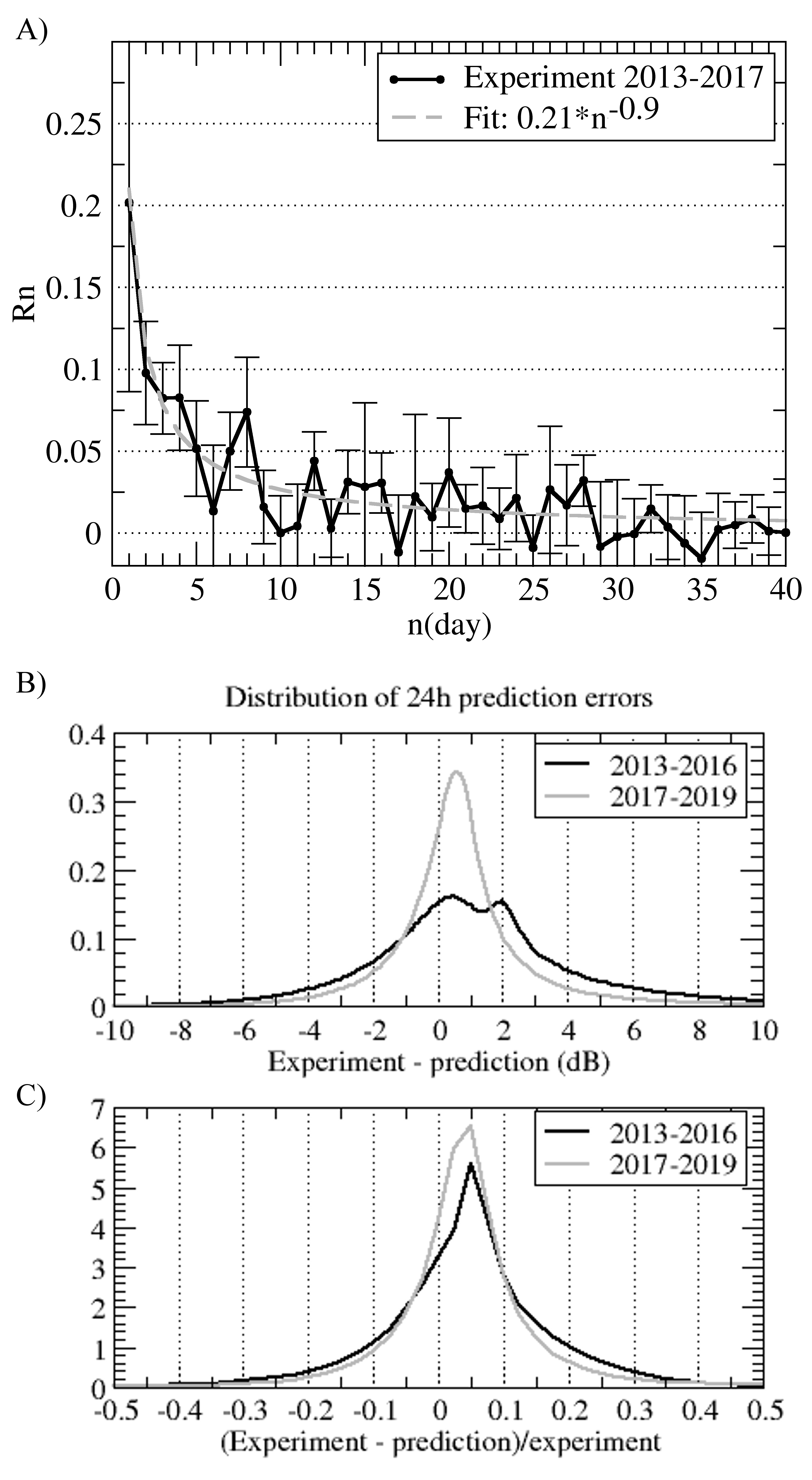
Figure 2: A) Weighting coefficients $R_{n}$ for the rough prediction model (Eq.(1,3)) calculated over the training dataset 2013-2016. The thick solid line corresponds to the averaged experimental $R_{n}$, thin line corresponds to RMS error of $R_{n}$. The smooth approximation of $R_{n}$ is shown by the green dashed line. B-C) Model (Eq.(1,3)) prediction accuracy : B) - the distribution of absolute prediction errors; C) - distribution of relative prediction errors. The black line in B-C is the distribution of errors over the training dataset (2013-2016), the gray line is the distribution of errors over the test dataset (2017-2018).

From Fig.2A we conclude that the effective averaging period for the rough predictive model of the noise is about 28 days, and the contribution of recent days is greater than the contribution of older ones. Fig.2A shows that the contribution of days older than 28-th is highly variable in sign, so we can neglect them and limit the calculations by 28-day history. The 28 days averaging period is in good agreement with the 30-day averaging period used for prediction of the riometric absorption at higher frequencies [14]. Stronger dynamics of the noise level at frequencies of 8–20 MHz, associated with background ionospheric dynamics, looks effectively reducing the averaging range and increases the contribution of recent days compared to an older ones into predicted value (Fig.2A).

To simplify the calculation of the coefficients, we approximated the dependence of the regression coefficients $R_{n}$ on the day number $n$ by the analytical function:

$$R_{n}\approx\left\{\begin{array}[]{l}0.21\cdot n^{-0.9},\,n\in[1..28]\\ 0,\,n>28\end{array}\right.$$ (3)

The approximation is shown in Fig.2A by dashed line. Using the constructed smoothed regression coefficients $R_{n}$ (Eq.(3)), the minimal noise level forecast is constructed for a day ahead, separately for the training dataset 2013-2016, and for the test dataset 2017-2018, and they are compared with experimental observations. The Fig.2B-C show the distribution of prediction errors for the day ahead according to the model Eq.(1,3) - for absolute errors (Fig.2B) and for relative errors (Fig.2C).

In Fig.2B-C shown that the average absolute and relative errors are biased for both the training and test datasets. Narrower error distribution over the test dataset can be explained by a lower level of solar activity and ionospheric disturbance in 2017-2018 compared with 2013-2016. Positive bias means that predicted noise level is lower than observed one. This bias is caused by using minimal noise level prediction instead of predicting the actual noise level.

When using the noise level for investigations of ionospheric absorption, the space weather effects usually cause lowering noise level [1, 2, 3, 4], so using the minimal noise level prediction makes the absorption identification technique less sensitive to random variations of the noise level.

Fine prediction model of the noise level

The rough prediction model described above predicts minimal noise level using minimal noise levels measured in previous days. Using this model allow us to identify the periods when noise level is lower than expected minimal value.

To predict the most expected noise level one requires an unbiased forecast, produced a zero mean error between experimental observations and forecast values. To build such an unbiased fine prediction of the noise, we used the rough noise model (described above) scaled to provide unbiased prediction.

The predicted value of the average noise level $f_{m,0}(t+\Delta T)$ with prediction time $\Delta T$ ahead the current moment $t$ in this approach can be presented as:

$$f_{m,0}(t+\Delta T)=M(t,\Delta T)f_{m,min}(t+\Delta T)$$ (4)

where $M(t,\Delta T)$ - some scaling factor. Since the experimental noise level $f_{e}(t)$ in this approach is proportional to the model one $f_{m,min}(t)$, the task of constructing an unbiased model is reduced to finding the optimal scaling function $M(t,\Delta T)$.

In proposed approach $M(t,\Delta T)$ is calculated as the weighted average of the ratios of the experimental noise level to the rough model of minimal noise level over a sufficiently long period. For calculations we use 12 days period with temporal resolution 15 minutes to predict noise level 12 hours ahead:

$$M(t,12h)=\sum_{\tau=0}^{12\,days}Q(\tau)\frac{f_{e}(t-\tau)}{f_{m,min}(t-\tau)}$$ (5)

where $Q(\tau)$ are regression coefficients to be found by fitting the experimental data $f_{e}(t;f_{sound},B_{m})$ by the model Eq.(4,5):

$$\varOmega_{2}(f_{sound},B_{m})=\int\left(f_{m,0}(t;f_{sound},B_{m})-f_{e}(t;f_{sound},B_{m})\right)^{2}dt=min$$ (6)

The 12 hours prediction interval is chosen as equidistant both from the current moment supported by the measurements $f_{e}(t)$ and from the 24 hour forecast value supported by the optimal prediction of the minimal noise level $f_{m,min}(t+24h)$ . We expect that the quality of the forecast at the moment $t+12h$ is the worst possible. Therefore, using the optimal weighting coefficients $Q(\tau)$ for this very forecast interval should improve the prediction accuracy.

The values of the regression coefficients $Q(\tau)$ are calculated based on the condition Eq.(6) over the test dataset (2013-2016). The variability of these coefficients from $\tau$, beam number $B_{m}$ and frequency $f_{0}$ is very high, which does not allow them to be analyzed directly. Therefore, we analyze the integral of the regression coefficients:

$$I(T)=\frac{1}{\sqrt{T}}\int_{0}^{T}Q(\tau)d\tau$$ (7)

also averaged over frequencies $f_{0}$ and beams $B_{m}$.

The position of the maximum of the function $I(T)$ corresponds to the characteristic time at which the coefficients of the regression model Eq.(4,5) are effective. The normalization of the integral by $\sqrt{T}^{-1}$ is used for compensating the effect of ’random walk process’ on the estimation of this characteristic time.

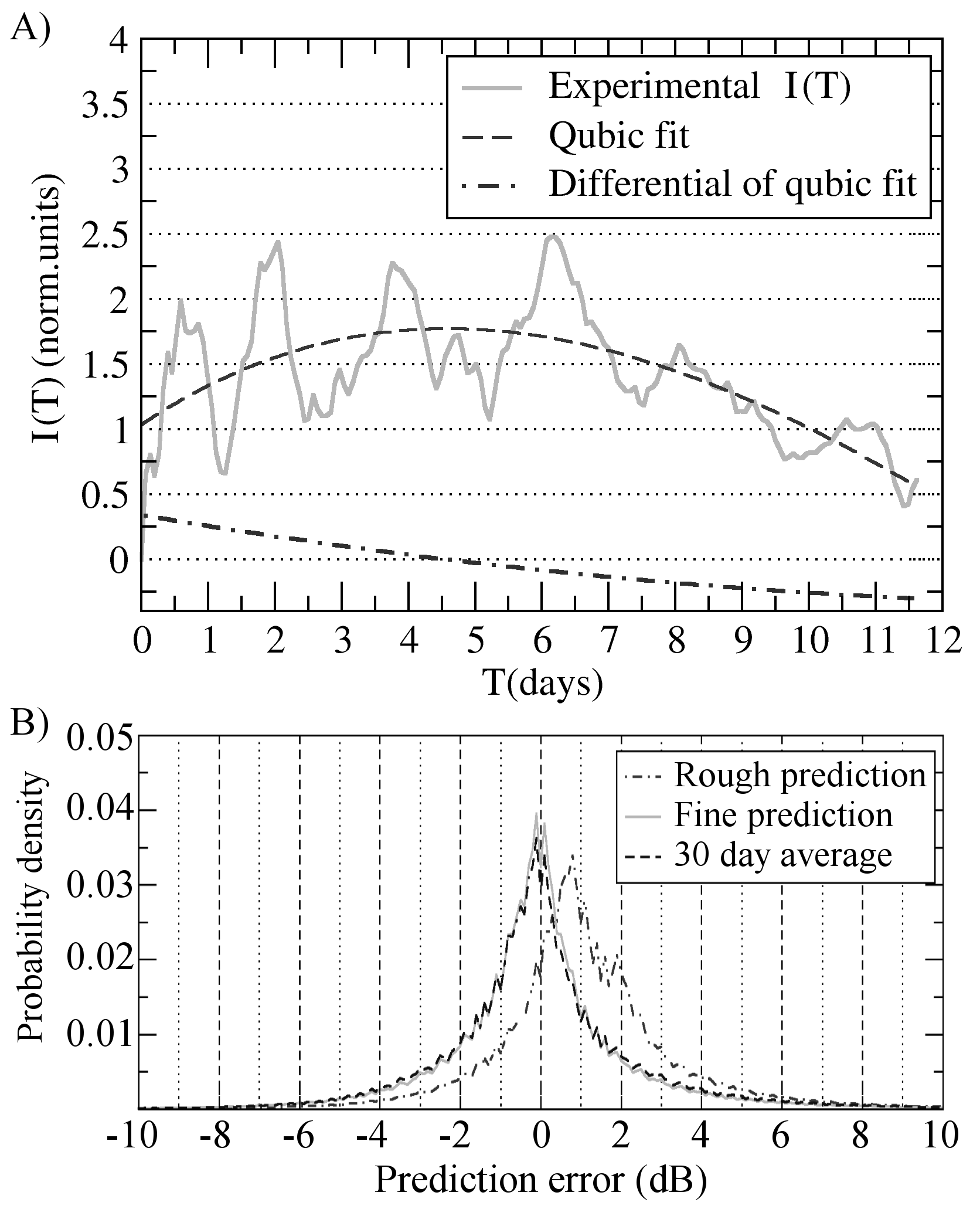
Figure 3: A) Dependence of $I(T)$ (Eq.(7)) on the delay $T$. The solid line is the experimental values of $I(T)$, the dashed line is its approximation by a smooth curve. The dot-dashed line corresponds to the expected average behavior of the regression coefficients $Q(\tau)$. B) The distributions of noise prediction errors for 6 hours ahead the current time after using 3 different techniques - rough prediction (dot-dashed line), 30 day average (dashed line) and fine prediction (solid line).

Fig.3A shows the behavior of $I(T)$ (Eq.(7), gray solid line) and its approximation by smooth cubic curve (dashed line).

In Fig.3A the dot-dashed line shows the expected model of the regression coefficients $Q(T)$, obtained by differentiating the smooth polynomial approximation of integral Eq.(7) (dashed line). From Fig.3A one can see that the main contribution to the regression prediction of the average noise level is given by previous 5 days, and their contribution decreases with from the most recent to the oldest days, and, in the first approximation, linearly. Thus, we use the simple analytical model of regression coefficients $Q(\tau)$:

$$Q(\tau)\approx\left\{\begin{array}[]{l}2\frac{T_{5d}-\tau}{T_{5d}};\tau<T_{5d}\\ 0;\tau\geq T_{5d}\end{array}\right.$$ (8)

where $T_{5d}$ is the optimal duration of regression, equal to 5 days.

By substituting Eq.(8) into Eq.(4,5) we obtain the fine prediction model in the final form:

$$f_{m,0}(t+\Delta T)=\sum_{\tau=0}^{T_{5d}}\left\{2\frac{T_{5d}-\tau}{T_{5d}}\cdot\frac{f_{e}(t-\tau)}{f_{m,min}(t-\tau)}\right\}f_{m,min}(t+\Delta T)$$ (9)

The constructed fine prediction model $f_{m,0}(t)$ uses rough prediction of the minimal noise level $f_{m,min}(t)$ obtained over previous 28 days and scale it using the previous 5 days data. So for functioning the fine model prediction requires 33 days of the historical observations.

Fig.3B shows the distribution of errors for various forecast techniques based on observations by the EKB ISTP SB RAS radar during 2013-2018. The figure shows a comparison of the 30-day average forecast (used in riometer measurements [14], as well as in some radar measurements [2], dashed line), the rough forecast of the minimal noise level described above (Eq.(1,3), dot-dashed line) and the fine forecast, described above (Eq.(9), solid line). It can be seen from the Fig.3B that the 30-day average forecast has the same error distribution as fine model has. This allows one to effectively use both forecasts for predicting actual noise level. The rough prediction model $f_{m,min}(t)$ is biased, and regularly underestimates the forecast value $f_{m,min}(t)$ relative to the experimental one $f_{e}(t)$. This bias approximately corresponds to single RMS error of using $f_{m,0}(t)$.

Thus, we can use $f_{m,min}(t)$ for detecting absorption periods, as the following condition:

$$f_{e}(t)<f_{m,min}(t)$$ (10)

The expected error of this detection technique can be determined from the distribution of errors (fig.3B) and is about 25%. To increase the accuracy of the detection we analyze each beam-frequency channel independently: for each frequency range $f_{sound}$ and each beam $B_{m}$. We select only the events that are simultaneously observed (i.e. lower than corresponding threshold level Eq.(10)) independently in five neighboring beams $B_{m}$ and in two independent frequencies $f_{sound}$. Using this approach should significantly decrease the detection error.

After detecting the absorption periods the exact value of the current absorption $A(t)$ is calculated from the fine prediction model 6 hours ahead based on 6 hours old measurements as following:

$$A(t)=\left\{\begin{array}[]{c}f_{e}(t)-f_{m,0}(t)[dB],\,f_{e}(t)<f_{m,0}(t)\\ 0,\,f_{e}(t)>f_{m,0}(t)\end{array}\right.$$ (11)

3 Statistical characteristics of detected absorption

The algorithm for automatic detection of absorption events and calculation of absorption intensity is used for statistical studies of spatio-temporal dynamics and frequency dependence of the detected absorption events. In Fig.4A shown the comparison of absorption distributions using two prediction models - fine forecast (Fig.4A, solid line, Eq.(10)) and 30-day average value (Fig.4A, dashed line). Absorption events are selected by Eq.(10). The comparison shows that both predictions produces nearly the same absorption distributions, and both techniques can be used to calculate the absorption.

Frequency dependence of the detected absorption

Traditionally it is believed that the absorption of radio waves vertically propagating in the ionosphere has a power-law frequency dependence [16, 17, 18, 19, 2, 4, 3]:

$$A[dB]=B\cdot f_{sound}^{\alpha}$$

Therefore, one of the possible approaches for verification of the developed technique is the analysis of frequency dependence of absorption based on large dataset. It has been evaluated in many papers, and usually $\alpha\approx-1.3\div-2.0$ [16, 17, 18, 19, 2, 4, 2].

By analogy with [4], to identify the power-law index and to increase the accuracy of its estimates, we select all the available observations of absorption events detected by EKB radar in 2013-2018 and transform them to equivalent vertical absorption (using algorithm described in [4]). To improve the accuracy we analyze only the cases when the absorption was detected simultaneously at two frequencies separated by more than 1.2 times. The frequency dependence $\alpha$ in each of the observations is determined as:

$$\alpha=\frac{log(\frac{A_{1}[dB]sin(E_{1})}{A_{2}[dB]\cdot sin(E_{2})})}{log(f_{1}[MHz]/f_{2}[MHz])}$$ (12)

where $A_{1},A_{2},f_{1},f_{2}$ are the logarithms of noise absorption at two frequencies, and these frequencies, respectively, $E_{1},E_{2}$ are the effective noise elevation angles calculated by algorithm presented in [4].

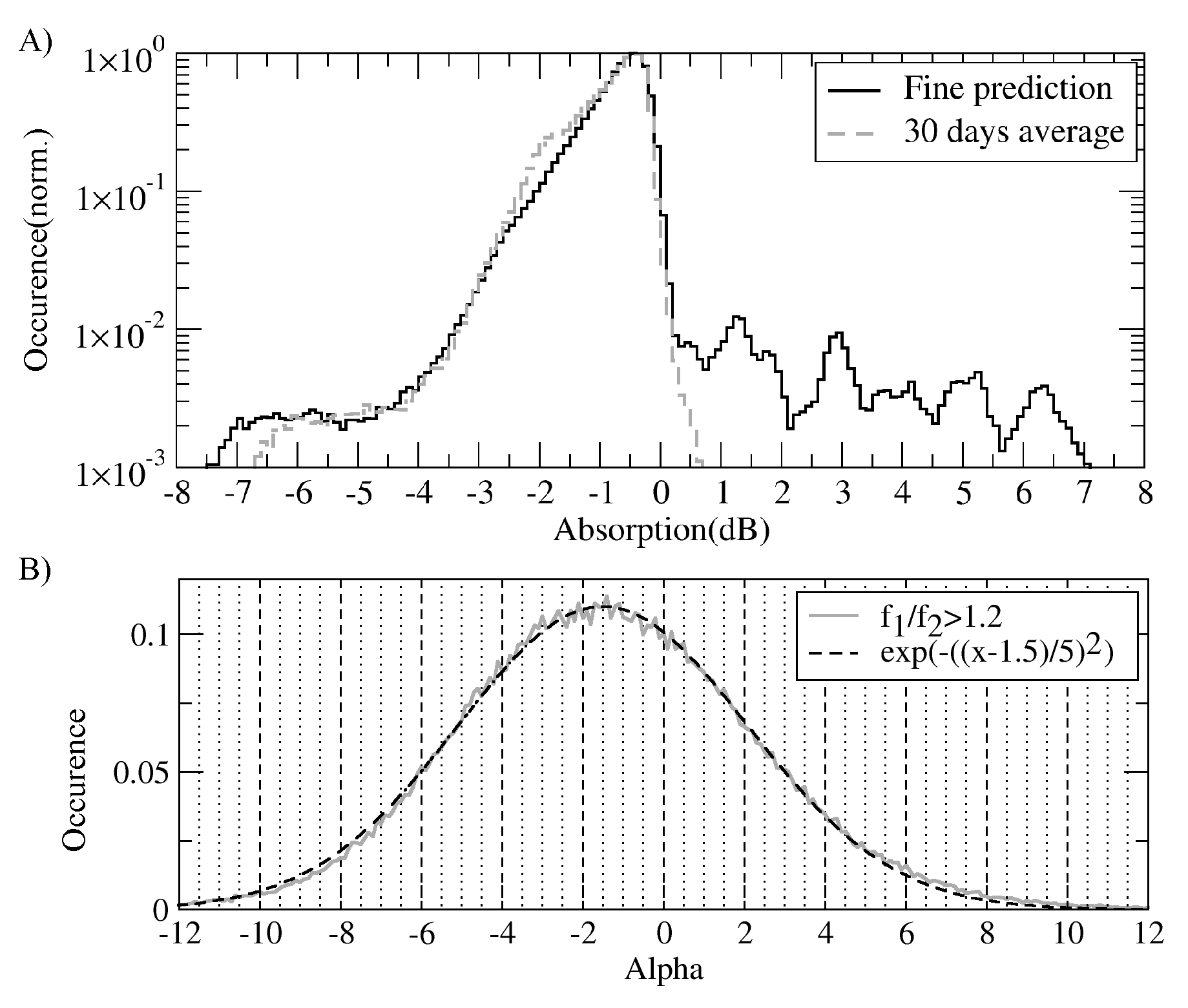
Figure 4: A) The distribution of absorption calulated using fine forecast and 30 day average; B) The distribution of the exponential absorption dependence $\alpha$ calculated over the absorption cases with the difference in the sounding frequencies $f_{1}/f_{2}>1.2$ (orange line) according to the formula Eq.(12). The dashed line shows the approximation of this distribution by the biased normal distribution.

The Fig.4B shows the distribution of $\alpha$, calculated according to Eq.(12) over more than 235 thousands of individual observations and the result of optimal fitting of this distribution by the normal distribution with a dispersion 5.0 and an average of -1.5. It can be seen from the figure that the frequency dependence with $\alpha=-1.5$ satisfactorily fits the experimental data and is in good agreement with the results obtained in papers [4, 18, 19, 17, 20].

Thus, the simultaneous observation of radio noise absorption at two spaced frequencies ($f_{1}/f_{2}>1.2$) can be interpreted as signal absorption in the ionosphere. This makes it possible to use the obtained noise prediction model and the detection algorithm for monitoring absorption in the ionosphere by coherent decameter radars.

The resulting absorption calculation algorithm is the following:

• At two frequencies and 5 neighboring beams, rough (Eq.(1,3)) and fine (Eq.(9)) forecasts of the noise level are separately made;

• If in all the cases simultaneously the measured noise is below its rough forecast (Eq.(10)) the moment is considered as an absorption event;

• In each of the frequency channel, the difference between the experimentally measured noise level and its fine forecast is calculated and reduced to the equivalent vertical absorption at 10MHz frequency according to:

  $$A(t)[dB]=\left\{\begin{array}[]{c}\left(f_{e}(t)-f_{m,0}(t)\right)sin(E(t))\left(\frac{f_{sound}(t)[MHz]}{10MHz}\right)^{1.5},\,f_{e}(t)<f_{m,0}(t)\\ 0,\,f_{e}(t)>f_{m,0}(t)\end{array}\right.$$ (13)

  where $f_{sound}(t)$ - sounding frequency and $E(t)$ is elevation calculated by method, described in [4].

• The resulting $A(t)$ is averaged over the 5 neighbor beams and 2 operational frequencies.

Spatio-temporal dynamics of detected absorption regions

Fig.5 shows the statistics of spatio-temporal absorption characteristics over 2013-2018 radar dataset.

It can be seen from Fig.4A that the most probable absorption level is about -0.65 dB. We have analyzed the spatio-temporal dynamics of absorption in the ranges 0..-0.65dB, -0.65..-1.3dB, -1.3..-2.6dB, ¡2.6dB, as well as a complete set of absorption events. The azimuthal dependence of the frequency of observation of absorption events Fig.5A-E and the dependence of the frequency of observation of absorption events on LST (Fig.5F-J) are studied. It can be seen from the Fig.5 that the absorption with weak and high amplitudes differ significantly. Cases of weak absorption (0..-1.3dB) are more often observed near the northern direction and are weakly dependent on local time. Strong events are practically independent of the beam number, and their daily dynamics (Fig.5H) correlates well with the daily dynamics of noise (Fig.5J, dashed line).

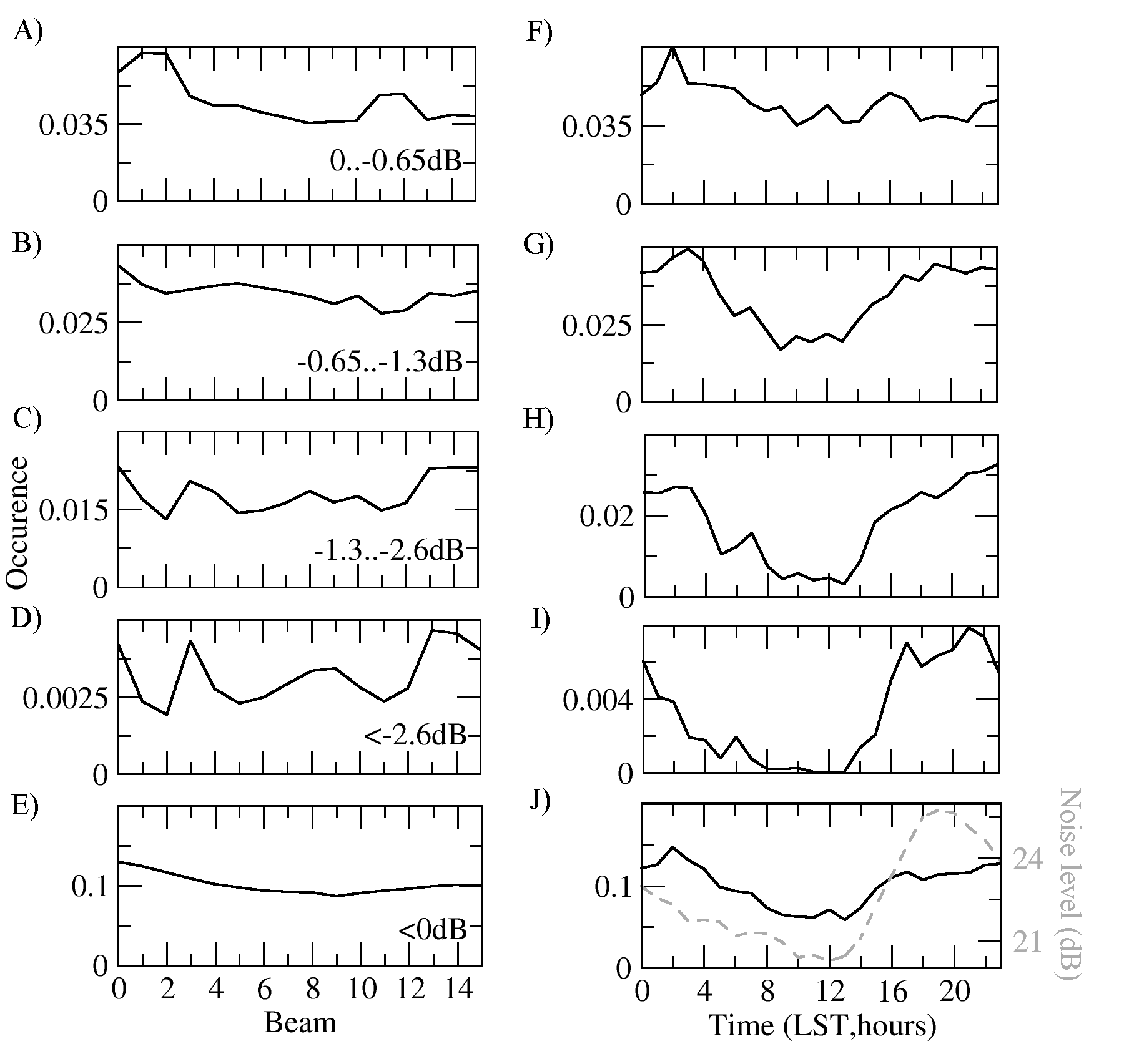
Figure 5: Spatio-temporal dynamics of absorption events with amplitudes 0..-0.65dB (A,F), -0.65..-1.3dB(B,G), -1.3..-2.6dB(C,H), ¡2.6dB(D,I), as well as a complete set of absorption events (E,J). A-E) Absorption events dependence on beam number; F-J) Absorption events dependence on local solar time; Gray dashed line at E) corresponds to the average noise level as a function of local solar time.

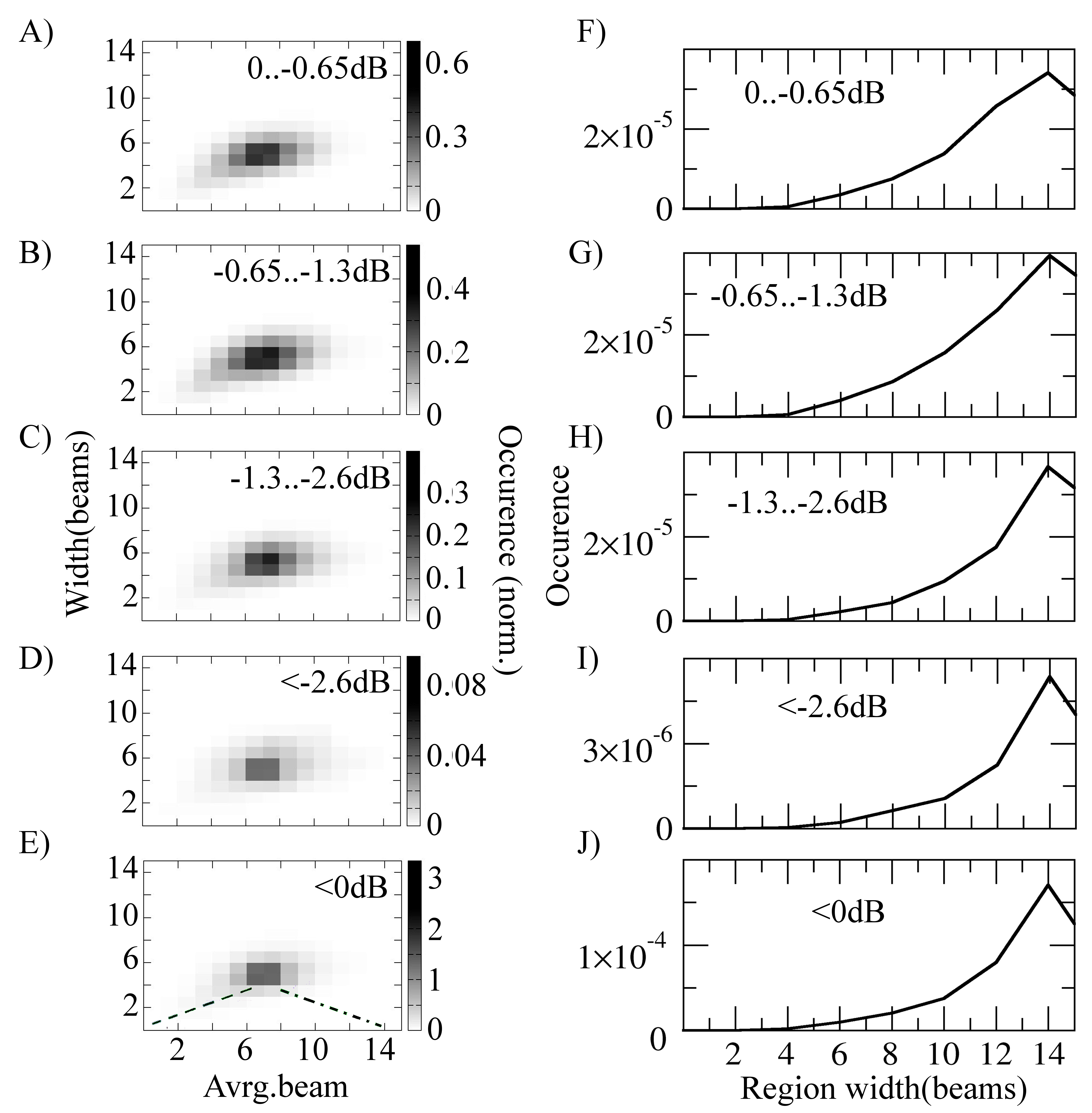
Figure 6: Spatial distributions of absorption events with amplitudes 0..-0.65dB (A,F), -0.65..-1.3dB(B,G), -1.3..-2.6dB(C,H), ¡2.6dB(D,I), as well as a complete set of absorption events (E,J). A-E) Distribution of absorption region locations and sizes (in number of beams); F-J) Distribution of average absorption region sizes (number of beams)

In Fig.6A-E shown the distributions of the average beam and the RMS of the sizes of the regions in which an absorption is observed with different intensity levels described above. To interpret the distribution of Fig.6A-E, the behavior of the average and RMS was simulated for different locations and sizes of the region. The simple simulation showed that when the region is located starting from the 0-th beam and changing is size from 1 to 15 beams it produces the dependence of RMS on average beam corresponding to the dashed line in Fig.6E. When the region is located starting from the 15th beam and changing its size from 1 to 15 beams, it produces the dependence of RMS on the average beam corresponding to the dot-dashed line in Fig.6E. From this results we can conclude that experimental observations at low absorption level (Fig.6A-B) correspond to the case when the absorption areas mainly include the 0th beam. The modeling showed that the average beam of the region in this case is equal to half the size of the region, which allows us to estimate the frequency of occurrence of absorbing regions with different sizes. Such an estimate is shown in Fig.6F-J. It can be seen that most frequently the absorbing region occupies the entire radar field-of-view, and the occurrence of smaller regions decreases with decreasing size of the region.

Smaller absorption events are frequently observed with smaller spatial sizes (Fig.8F-G), and higher absorption events - with larger spatial sizes (Fig.8H-J).

From the figure one can conclude that some cases of absorption events with small amplitudes (0 ..-1.3dB) have smaller spatial scales and are concentrated on northern beams. The observations with high absorption amplitudes are most often large-scale.

In Fig.7A are shown distributions of absorption events by duration. As one can see, the observed events usually are shorter than 16 hours, that can be related with mid-latitude location of the radar. For high-latitude radars the durations can be longer.

In Fig.7B are shown the average absorption amplitudes over different absorption events. As one can see, the most powerful events usually shorter than less powerful ones. From the figure ane can see that powerful events up to -2dB usually are abserved not longer than 1-1.5 hours.

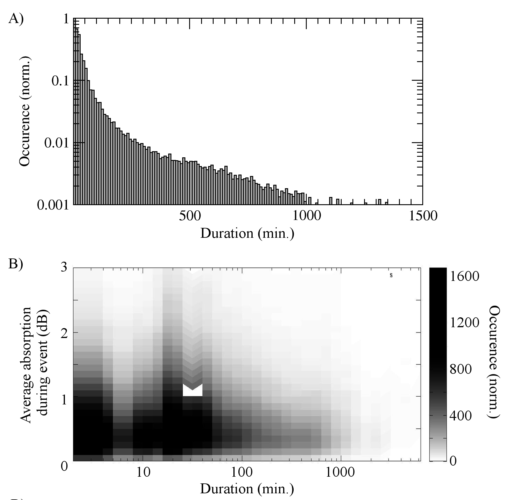
Figure 7: A) Distribution of absorption events by duration; B) Average absorption amplitudes as function of absorption event duration

4 Case comparison of the prediction algorithms in different cases.

Short-lived absorption case

Fig.8A,C shows an example of different algorithms operation during two solar X-ray flares: rough and fine forecasts as well as traditional 30 day average forecast. Fig.8B,D shows the corresponding examples of the calculated absorption level, reduced to 10MHz frequency and to the vertical propagation of a radio wave. It can be seen from the figures that a rough forecast is often below the noise level and its forecasts (fine and 30-day average), which leads to the fact that the use of an fine forecast and a 30-day averaging to determine the absorption in some cases will give fairly close results, which is observed experimentally (Fig.3B).

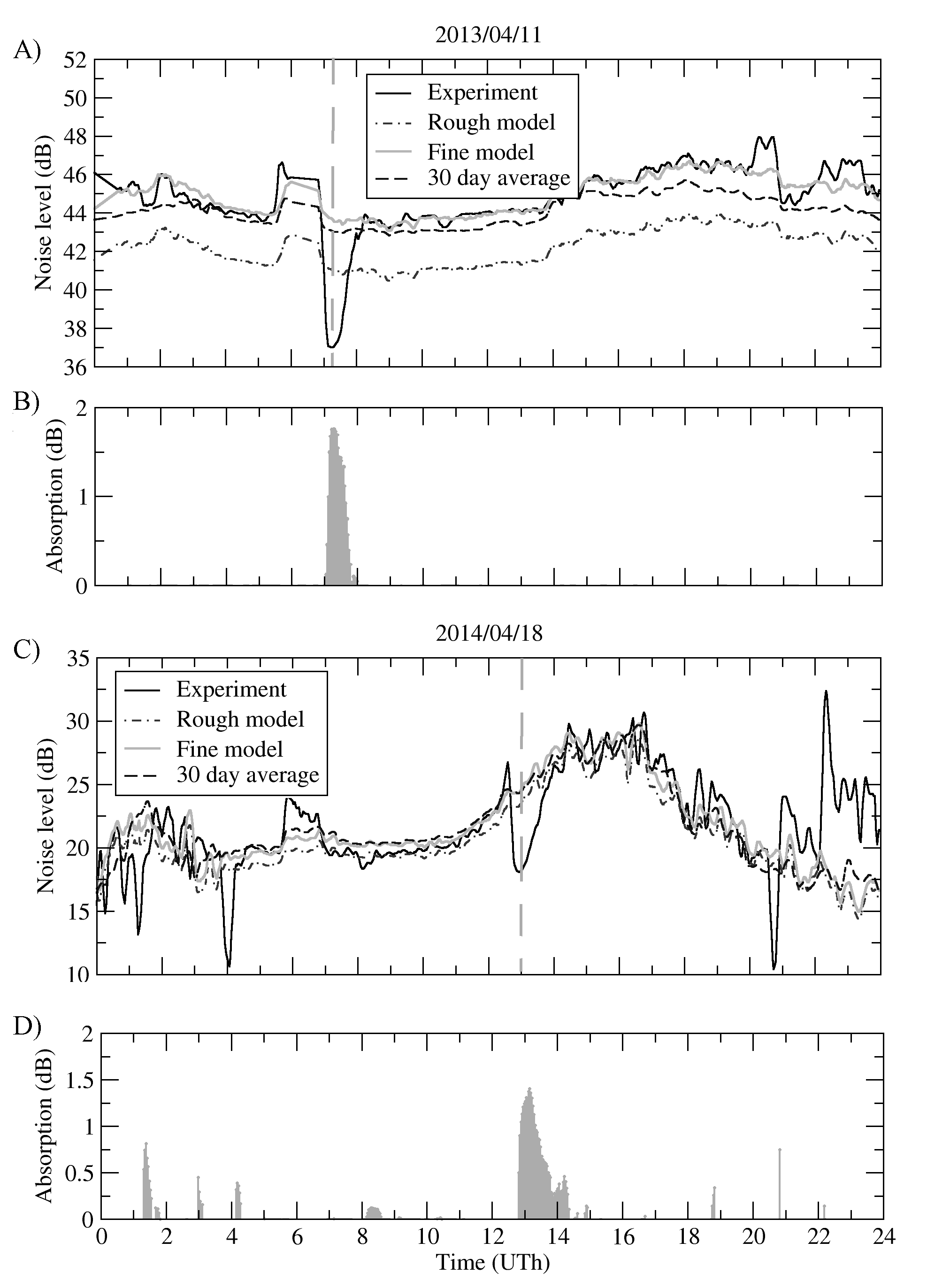
Figure 8: The operation of the prediction algorithms during two solar X-ray flares - 04/11/2013 (A-B) and 18/04/2014 (C-D) (the moments of the flares are marked by vertical dashed lines). A,C) - noise measurements and different predictions; B,D) - absorption level calculated by the algorithm.

As one can see from 8A, in some cases the fine prediction algorithm predict noise level better than traditional 30-day forecast. From 8C one can also see that the rough prediction is expectedly about 1 dB lower than actual noise level, and therefore can be used for detecting the absorption cases. At high latitudes, for which riometric and radar [3] absorption are large, using the traditional 30 day average forecast instead of the fine prediction looks equivalent. At the middle latitudes the absorption is smaller and one should use more accurate fine forecast.

Long-lived absorption case

Fig.9 shows prediction algorithms during the September 10-11, 2017 event related with Coronal mass ejection event[2]. The Fig.9A-B shows the noise measurements and their prediction at 10 and 11MHz. As one can see from Fig.9B, the traditional 30-day average algorithm (dashed line) in this case looks working better than fine prediction algorithm (thin solid line). This can be related with using 5 days adaptation for fine prediction, that does not work well in case of long-lasting absorption events. So the fine prediction can be used only in short-lasting events, for example, during X-ray solar flares [1, 4]. Fig.9C shows the corresponding example of the calculated absorption level, reduced to 10MHz frequency and to the vertical propagation of a radio wave. It also takes into account observations at both frequencies and at five neighboring beams.

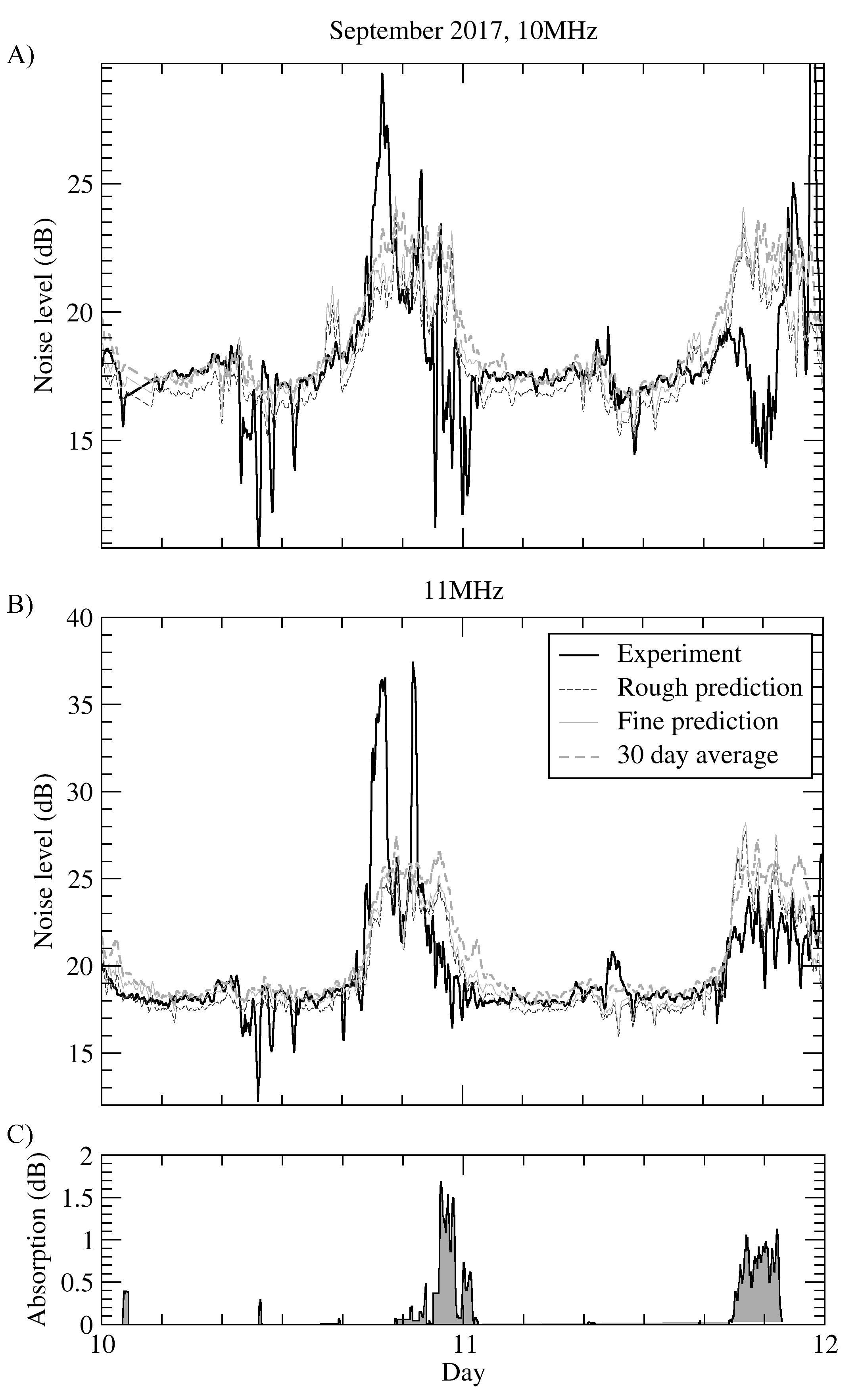
Figure 9: An example of the operation of noise prediction algorithms during the September 10-11, 2017 event. A) observations at 10MHz sounding frequency B) is observations at 11 MHz frequency. C) is absorption level detected by final algorithm Eq.(13).

As shows the qualitative case analysis above, the traditional 30-day averaging can be used for prediction noise level in long-lasting absorption cases, for fine prediction of noise level in short-lasting events it is recommended to use fine prediction algorithm. Rough prediction algorithm can be used for detection the absorption in both cases.

5 Conclusion

A statistical analysis of the dynamics of noise variations on a coherent decameter radar EKB ISTP SB RAS, related to the radiowaves absorption in the lower part of the ionosphere, was carried out for the first time. To carry out the analysis, a method for predicting the minimal noise level based on the optimal autoregression was implemented. The autoregression is based in the minimal noise measurements over the previous 28 days, and used to forecast the minimal noise level for 1 day ahead the most accurately. An analytical formula (Eq.(3)) is given for the obtained coefficients.

Based on the optimal forecast of the minimal noise level, a method is proposed for the optimal (fine) forecast of the noise level based on the calibration (scaling) of the predicted minimal noise level. The analysis of the complete data set 2013-2018 showed that the optimal forecast can be build by using calibration over the previous 5 days. The accuracy of the constructed fine forecast is compared with accuracy of 30 days average noise value. The comparison showed that the distribution of prediction errors is almost identical (Fig.3B) for these two methods.

A case analysis of several events showed that in the case of short-term absorption cases, the fine prediction model can be more accurate than the traditional riometric algorithm (Fig.8A), and during long-term absorption cases, the traditional riometric algorithm scan be more accurate (Fig.9 A-B). So in the cases of analysis high-latitude data with frequent absorption the riometric algorithm looks preferable, and in the case of mid-latitude data and short-living events - fine prediction algorithm looks preferable.

Based on the analysis of September 10-11, 2017 case, it was shown that at different frequencies the shape of the absorption effect may vary (Fig.9 A-B), which leads to the need to use measurements at several frequencies to more reliably detect the cases of absorption.

As a result, a two-frequency detection technique is proposed for detecting the absorption cases, based on simultaneously detecting a decrease in noise level below the rough minimal noise forecast at two independent frequencies and five neighboring radar beams. The absorption is estimated by calculating the difference in the measured noise level relative to the fine noise level forecast and averaging the effect over sounding frequencies and neighbor beams, taking into account the frequency and elevation angle dependencies of the absorption and reduction the absorption value to 10MHz frequency in analogy to [4].

Statistical analysis of two-frequency experiments in the period 2013-2018 is made. The analysis shows the exponential frequency dependence of the absorption with -1.5 power coefficient (Fig.4B). This value corresponds well with the data of other observations and models [16, 17, 18, 19, 4] and allows to use the proposed model for detecting and estimating the absorption level over the large noise dataset obtained at EKB ISTP SB RAS radar in 2013-2018.

Based on a large amount of statistical data (2013-2018), it was shown that the average daily diurnal variation of the vertical absorption level at 10 MHz does not depend on local time for abosrption events with smaller amplitude (0..-1.3dB) and looks close to the variations of the average durinal variation of the noise level (Fig.5C,E) at high amplitudes.

Based on the statistical analysis of the spatial structure of the absorbing regions over 2013-2018, it was shown that a significant part of the absorption events with small amplitude (0..-1.3dB) corresponds to high-latitude absorption(Fig.6F-G), and high amplitude absorption events (stonger than -1.3dB) corresponds to large-scale events comparable in size to the radar field-of-view (Fig.6H-J) - about 50 degrees in azimuth. This allows to suggest that observed strong absorption events at nighttime can be significantly affected by radiowave propagation effects, requires more correct elevation angle calculations (significantly changing calculated absorption level) and should be interpreted as absorption very carefully.

It is important to note that by definition the presented technique can not be used for investigations of regular absorption variations with 24 hours periodicity, and is useful for investigating irregular, preferably short-living events.

References

References

- [1] O. I. Berngardt, J. M. Ruohoniemi, N. Nishitani, S. G. Shepherd, W. A. Bristow, E. S. Miller, Attenuation of decameter wavelength sky noise during x–ray solar flares in 2013–2017 based on the observations of midlatitude HF radars, Journal of Atmospheric and Solar-Terrestrial Physics 173 (2018) 1 – 13. doi:10.1016/j.jastp.2018.03.022
- [2] E. C. Bland, E. Heino, M. J. Kosch, N. Partamies, SuperDARN radar–derived HF radio attenuation during the September 2017 solar proton events, Space Weather doi:10.1029/2018sw001916
- [3] E. C. Bland, N. Partamies, E. Heino, A. S. Yukimatu, H. Miyaoka, Energetic electron precipitation occurrence rates determined using the Syowa East SuperDARN radar, Journal of Geophysical Research: Space Physics 124(7). 6253–6265, 2019, doi:10.1029/2018JA026437
- [4] O. Berngardt, J. Ruohoniemi, J.-P. St.Maurice, A. Marchaudon, M. Kosch, A. Yukimatu, N. Nishitani, S. Shepherd, M. Marcucci, H. Hu, T. Nagatsuma, M. Lester, Space Weather 17 (6) (2019) 907–924. doi:10.1029/2018SW002130
- [5] S. Chakraborty, J. B. H. Baker, J. M. Ruohoniemi, B. Kunduri, N. Nishitani, S. G. Shepherd, A Study of SuperDARN Response to Co-occurring Space Weather Phenomena, Space Weather, 2019 doi:10.1029/2019SW002179
- [6] D. Watanabe, N. Nishitani, Study of ionospheric disturbances during solar flare events using the SuperDARN Hokkaido radar, Advances in Polar Science 24 (1) (2013) 12–18. doi:10.3724/sp.j.1085.2013.00012
- [7] R. A. D. Fiori, A. V. Koustov, S. Chakraborty, J. M. Ruohoniemi, D. W. Danskin, D. H. Boteler, S. G. Shepherd, Examining the potential of the Super Dual Auroral Radar Network for monitoring the space weather impact of solar X–ray flares, Space Weather doi:10.1029/2018sw001905
- [8] M. Lester, P. J. Chapman, S. W. H. Cowley, S. J. Crooks, J. A. Davies, P. Hamadyk, K. A. McWilliams, S. E. Milan, M. J. Parsons, D. B. Payne, E. C. Thomas, J. D. Thornhill, N. M. Wade, T. K. Yeoman, R. J. Barnes, Stereo CUTLASS - A new capability for the SuperDARN HF radars, Annales Geophysicae 22 (2) (2004) 459–473. doi:10.5194/angeo-22-459-2004
- [9] R. Greenwald, K. B. Baker, J. R. Dudeney, M. Pinnock, T. Jones, E. Thomas, J.-P. Villain, J. C. Cerisier, C. Senior, C. Hanuise, R. D. Hunsucker, G. Sofko, J. Koehler, E. Nielsen, R. Pellinen, A. Walker, N. Sato, H. Yamagishi, Darn/Superdarn: A Global View of the Dynamics of High–Lattitude Convection, Space Science Reviews 71 (1995) 761–796. doi:10.1007/BF00751350
- [10] G. Chisham, M. Lester, S. Milan, M. Freeman, W. Bristow, K. McWilliams, J. Ruohoniemi, T. Yeoman, P. Dyson, R. Greenwald, T. Kikuchi, M. Pinnock, J. Rash, N. Sato, G. Sofko, J.-P. Villain, A. Walker, A decade of the Super Dual Auroral Radar Network (SuperDARN): scientific achievements, new techniques and future directions, Surveys in Geophysics (28) (2007) 33–109. doi:10.1007/s10712-007-9017-8
- [11] N. Nishitani, J. Ruohoniemi, M. Lester, J. B. H. Baker, A. V. Koustov, S. G. Shepherd, G. Chisham, T. Hori, E. G. Thomas, R. A. Makarevich, A. Marchaudon, P. Ponomarenko, J. A. Wild, S. E. Milan, W. A. Bristow, J. Devlin, E. Miller, R. A. Greenwald, T. Ogawa, T. Kikuchi, Review of the accomplishments of mid-latitude super dual auroral radar network (superdarn) hf radars, Progress in Earth and Planetary Science 6 (1) (2019) 27. doi:10.1186/s40645-019-0270-5
- [12] ITU-R P.372-13, Recommendation ITU-R P.372-13. Radio noise (09 2016). https://www.itu.int/rec/R-REC-P.372-13-201609-I/en
- [13] P. Ponomarenko, B. Iserhienrhien, J.-P. St.-Maurice, Morphology and possible origins of near-range oblique HF backscatter at high and midlatitudes, Radio Science 51 (6) (2016) 718–730. doi:10.1002/2016rs006088
- [14] R. Heisler, G. L. Hower, Riometer quiet day curves, Journal of Geophysical Research (1896-1977) 72 (21) (1967) 5485–5490. doi:10.1029/JZ072i021p05485
- [15] U. of Calgary, CANOPUS Quiet Day Curve Generation, http://aurora.phys.ucalgary.ca/norstar/rio/doc/CANOPUS_Riometer_Baselining.pdf.
- [16] J. Hargreaves, Auroral radio absorption: The prediction question, Advances in Space Research 45 (9) (2010) 1075 – 1092. doi:10.1016/j.asr.2009.10.026
- [17] E. A. Schumer, Improved modeling of midlatitude D–region ionospheric absorption of high frequency radio signals during solar X–ray flares, Ph.d. dissertation, Air Force Institute of Technology (2010).
- [18] DRAP Documentation, Global D–region absorption prediction documentation, accessed September,2018 (2010). https://www.swpc.noaa.gov/content/global-d-region-absorption-prediction-documentation
- [19] Akmaev, R. A., DRAP Model Validation: I.Scientific Report (2010). https://www.ngdc.noaa.gov/stp/drap/DRAP-V-Report1.pdf
- [20] N. C. Rogers, F. Honary, Assimilation of real–time riometer measurements into models of 30 MHz polar cap absorption, J. Space Weather Space Clim. 5 (2015) A8. doi:10.1051/swsc/2015009.