A lower-bound estimate of the Lyapunov dimension
for the global attractor of the Lorenz system

Abstract

In this short report, for the classical Lorenz attractor we demonstrate the applications of the Pyragas time-delayed feedback control technique and Leonov analytical method for the Lyapunov dimension estimation and verification of the Eden’s conjecture. The problem of reliable numerical computation of the finite-time Lyapunov dimension along the trajectories over large time intervals is discussed.

I Lorenz attractor and Pyragas stabilization of embedded unstable periodic orbits

Consider the classical Lorenz system Lorenz-1963

$$\begin{cases}\dot{x}=-\sigma(x-y),\\ \dot{y}=rx-y-xz,\\ \dot{z}=-bz+xy,\end{cases}$$ (1)

with physically sound parameters $\sigma,r>0$, and $b\in[0,4]$. For $r<1$ it has only one globally stable equilibrium $S_{0}=\big{(}0,\,0,\,0\big{)}$, and for $r>1$ the equilibrium $S_{0}$ turns into a saddle, while two new symmetric equilibria appear:

$$S_{\pm}=\big{(}\pm\sqrt{b(r-1)},\,\pm\sqrt{b(r-1)},\,r-1\big{)},$$ (2)

which stability depends on the values of parameters.

System (1) is dissipative in the sense of Levinson (see e.g. (LeonovKM-2015-EPJST, )), i.e. there exist a global bounded absorbing set containing global attractor $\mathcal{A}_{\rm glob}$, and in some cases this attractor exhibits chaotic behavior. For some values of parameters, it is possible to observe a case of multistability, when the global attractor consists of several local attractors. To get a visualization of such attractors one needs to choose an initial point in the basin of attraction of a particular attractor and observe how the trajectory, starting from this initial point, after a transient process visualizes the attractor: an attractor is called a self-excited attractor if its basin of attraction intersects with any open neighborhood of an equilibrium, otherwise, it is called a hidden attractor (LeonovKV-2011-PLA, ; LeonovK-2013-IJBC, ; LeonovKM-2015-EPJST, ; Kuznetsov-2016, ). It was discovered numerically by E. Lorenz that in the phase space of system (1) with parameters $r=28$, $\sigma=10$, $b=8/3$ there exist a chaotic attractor $\mathcal{A}$, which is self-excited with respect to all equilibria $S_{0}$, $S_{\pm}$.

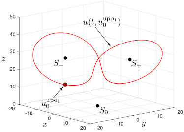
(a)

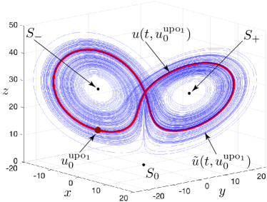
(b)

Figure 1: Period-1 UPO $u^{\rm upo_{1}}(t)$ (red, period $\tau_{1}=1.5586$) stabilized using UDFC method, and pseudo-trajectory $\tilde{u}(t,u^{\rm upo_{1}}_{0})$ (blue, $t\in[0,100]$) in system (1) with parameters $r=28$, $\sigma=10$, $b=8/3$.

The ”skeleton” of a chaotic attractor comprises embedded unstable periodic orbits (UPOs) (see e.g. (AfraimovicBSh-1977, ; AuerbachCEGP-1987, ; Cvitanovic-1991, )), and one of the effective methods among others for the computation of UPOs is the delay feedback control (DFC) approach, suggested by K. Pyragas (Pyragas-1992, ) (see also discussions in (KuznetsovLS-2015-IFAC, ; ChenY-1999, ; LehnertHFGFS-2011, )). This approach allows Pyragas and his progeny to stabilize and study UPOs in various chaotic dynamical systems. Nevertheless, some general analytical results have been obtained HootonA-2012 , showing that DFC has a certain limitation, called the odd number limitation (ONL), which is connected with an odd number of real Floquet multipliers larger than unity. In order to overcome ONL, later Pyragas suggested a modification of the classical DFC technique, which was called the unstable delayed feedback control (UDFC) Pyragas-2001 .

Rewrite system (1) in a general form

$$\dot{u}=f(u).$$ (3)

Let $u^{\rm upo}(t,u^{\rm upo_{1}}_{0})$ be its UPO with period $\tau>0$, $u^{\rm upo}(t-\tau,u^{\rm upo_{1}}_{0})=u^{\rm upo}(t,u^{\rm upo_{1}}_{0})$, and initial condition $u^{\rm upo_{1}}_{0}=u^{\rm upo}(0,u^{\rm upo_{1}}_{0})$. To compute the UPO and overcome ONL, we add the UDFC in the following form:

$$\dot{u}(t) =f(u(t))+KB\,\big{[}F_{N}(t)+w(t)\big{]},$$ (4)

$$\dot{w}(t) =\lambda_{c}^{0}w(t)+(\lambda_{c}^{0}-\lambda_{c}^{\infty})F_{N}(t),$$

$$F_{N}(t) =C^{*}u(t)-(1\!-\!R)\sum_{k=1}^{N}R^{k-1}C^{*}u(t-kT),$$

where $0\leq R<1$ is an extended DFC parameter, $N=1,2,\ldots,\infty$ defines the number of previous states involved in delayed feedback function $F_{N}(t)$, $\lambda_{c}^{0}>0$, and $\lambda_{c}^{\infty}<0$ are additional unstable degree of freedom parameters, $B,C$ are vectors and $K>0$ is a feedback gain. For initial condition $u^{\rm upo_{1}}_{0}$ and $T=\tau$ we have

$$F_{N}(t)\equiv 0,\ w(t)\equiv 0,$$

and, thus, the solution of system (4) coincides with the periodic solution of initial system (3).

For the Lorenz system (1) with parameters $r=28$, $\sigma=10$, $b=8/3$ using (4) with $B^{*}=\left(0,1,0\right)$, $C^{*}=\left(0,1,0\right)$, $R=0.7$, $N=100$, $K=3.5$, $\lambda^{0}_{c}=0.1$, $\lambda^{\infty}_{c}=-2$, one can stabilize a period-1 UPO $u^{\rm upo_{1}}(t,u_{0})$ with period $\tau_{1}=1.5586$ from the initial point $u_{0}=(1,1,1)$, $w_{0}=0$ (see Fig. 1). Results of this experiment could be repeated using various other numerical approaches (see e.g. Viswanath-2001 ; Budanov-2018 ; PchelintsevPY-2019-LorenzUpo ), and are in agreement with similar results on the existence of UPOs embedded in the Lorenz attractor GaliasT-2008-LorenzUpo ; BarrioDT-2015-LorenzUpo . However, the Pyragas procedure, in general, is more convenient for UPOs numerical visualization.

For the initial point $u^{\rm upo_{1}}_{0}\approx(-6.2262,-11.0027,13.0515)$ on the UPO $u^{\rm upo_{1}}(t)=u(t,u^{\rm upo_{1}}_{0})$ we numerically compute the trajectory of system (4) without the stabilization (i.e. with $K=0$) on the time interval $[0,T=100]$ (see Fig. 1b). We denote it by $\tilde{u}(t,u^{\rm upo_{1}}_{0})$ to distinguish this pseudo-trajectory from the periodic orbit $u(t,u^{\rm upo_{1}}_{0})$. One can see that on the initial small time interval $[0,T_{1}\approx 11]$, even without the control, the obtained trajectory $\tilde{u}(t,u^{\rm upo_{1}}_{0})$ traces approximately the ”true” periodic orbit $u(t,u^{\rm upo_{1}}_{0})$. But for $t>T_{1}$, without a control, the trajectory $\tilde{u}(t,u^{\rm upo_{1}}_{0})$ diverge from $u^{\rm upo_{1}}(t,u^{\rm upo_{1}}_{0})$ and visualize a local chaotic attractor $\mathcal{A}$.

Remark that in numerical computation of trajectory over a finite-time interval it is also difficult to distinguish a sustained chaos from a transient chaos (a transient chaotic set in the phase space, which can persist for a long time) GrebogiOY-1983 . This challenging task is related to an open problem about the existence of a hidden chaotic attractor in the Lorenz system (1) (see e.g. discussions in LeonovK-2015-AMC ; LeonovKM-2015-EPJST ; ChenKLM-2017-IJBC ; SprottM-2018-HA ).

II Lyapunov dimension estimation and Eden conjecture

Following Kuznetsov-2016-PLA ; KuznetsovLMPS-2018 , let us outline the concept of the finite-time Lyapunov dimension, which is convenient for carrying out numerical experiments with finite time.

For a fixed $t\geq 0$ let us consider the map $u(t,\cdot):\mathbb{R}^{3}\to\mathbb{R}^{3}$ defined by the shift operator along the solutions of system (1): $u(t,u_{0})$, $u_{0}\in\mathbb{R}^{3}$. Since system (1) possesses an absorbing set, the existence and uniqueness of solutions of system (1) for $t\in[0,+\infty)$ take place and, therefore, the system generates a dynamical system $\big{(}\{u(t,\cdot)\}_{t\geq 0},(\mathbb{R}^{3},|\cdot|)\big{)}$.

Consider linearization of system (1) along the solution $u(t,u_{0})$ and its $3\!\times\!3$ fundamental matrix of solutions $\Phi(t,u_{0})$: $\dot{\Phi}(t,u_{0})=Df((u(t,u_{0}))\Phi(t,u_{0})$, where $\Phi(0,u_{0})\leavevmode\nobreak\ =\leavevmode\nobreak\ I$ is a unit $3\!\times\!3$ matrix. Denote by $\sigma_{i}(t,u_{0})=\sigma_{i}(\Phi(t,u_{0}))$, $i=1,2,3$, the singular values of $\Phi(t,u_{0})$ (i.e. the square roots of the eigenvalues of the symmetric matrix $\Phi(t,u_{0})^{*}\Phi(t,u_{0})$ with respect to their algebraic multiplicity), ordered so that $\sigma_{1}(t,u_{0})\geq\sigma_{2}(t,u_{0})\geq\sigma_{3}(t,u_{0})>0$ for any $u_{0}\in\mathbb{R}^{3}$ and $t>0$.

Consider a set of finite-time Lyapunov exponents at the point $u_{0}$:

$$\operatorname{LE}_{i}(t,u_{0})=\frac{1}{t}\ln\sigma_{i}(t,u_{0}),\ t>0,\quad i=1,2,3.$$ (5)

Here, the set $\{\operatorname{LE}_{i}(t,u_{0})\}_{i=1}^{3}$ is ordered by decreasing (i.e. $\operatorname{LE}_{1}(t,u_{0})\geq\operatorname{LE}_{2}(t,u_{0})\geq\operatorname{LE}_{3}(t,u_{0})$ for all $t>0$). The finite-time local Lyapunov dimension Kuznetsov-2016-PLA ; KuznetsovLMPS-2018 can be defined via an analog of the Kaplan-Yorke formula with respect to the set of ordered finite-time Lyapunov exponents $\{\operatorname{LE}_{i}(t,u_{0})\}_{i=1}^{3}$:

$$\dim_{\rm L}(t,u_{0})\!=\!j(t,u_{0})+\tfrac{\operatorname{LE}_{1}\!(t,u_{0})+\cdot\cdot+\operatorname{LE}_{j(,u_{0})}\!(t,u_{0})}{|\operatorname{LE}_{j(t,u_{0})\!+\!1}(t,u_{0})|},$$ (6)

where $j(t,u_{0})=\max\{m:\sum_{i=1}^{m}\operatorname{LE}_{i}(t,u_{0})\geq 0\}$. Then the finite-time Lyapunov dimension of dynamical system with respect to a set $\mathcal{A}$ is defined as:

$$\dim_{\rm L}(t,\mathcal{A})=\sup\limits_{u_{0}\in\mathcal{A}}\dim_{\rm L}(t,u_{0}).$$ (7)

The Douady–Oesterlé theorem DouadyO-1980 implies that for any fixed $t>0$ the finite-time Lyapunov dimension on a compact invariant set $\mathcal{A}$, defined by (7), is an upper estimate of the Hausdorff dimension: $\dim_{\rm H}\mathcal{A}\leq\dim_{\rm L}(t,\mathcal{A})$. The best estimation is called the Lyapunov dimension Kuznetsov-2016-PLA

$$\dim_{\rm L}\mathcal{A}=\inf_{t>0}\sup\limits_{u_{0}\in\mathcal{A}}\dim_{\rm L}(t,u_{0})=\\ =\liminf_{t\to+\infty}\sup\limits_{u_{0}\in\mathcal{A}}\dim_{\rm L}(t,u_{0}).$$

We use the adaptive algorithm for the computation of the finite-time Lyapunov dimension and exponents for trajectories on the local attractor $\mathcal{A}$ KuznetsovLMPS-2018 . In order to distinguish the corresponding values for the stabilized UPO $u(t,u^{\rm upo_{1}}_{0})$ with a period $\tau_{1}=1.5586$ and for the pseudo-trajectory $\tilde{u}(t,u^{\rm upo_{1}}_{0})$ computed without Pyragas stabilization in our experiment we use the following notations for finite-time Lyapunov dimensions: $\dim_{\rm L}(u(t,\cdot),u^{\rm upo_{1}}_{0})$ and $\dim_{\rm L}(\tilde{u}(t,\cdot),u^{\rm upo_{1}}_{0})$, respectively.

(a)

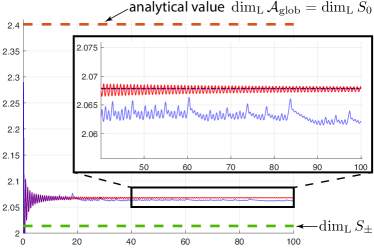
(b)

Figure 2: Evolution of FTLDs $\dim_{\rm L}(u(t,\cdot),u^{\rm upo_{1}}_{0})$ (red) and $\dim_{\rm L}(\tilde{u}(t,\cdot),u^{\rm upo_{1}}_{0})$ (blue) computed on the time interval $t\in[0,100]$ along the UPO $u^{\rm upo_{1}}(t)=u(t,u^{\rm upo_{1}}_{0})$ (red) and the trajectory $\tilde{u}(t,u^{\rm upo_{1}}_{0})$ (blue) integrated without stabilization, respectively. Both trajectories start from the point $u^{\rm upo_{1}}_{0}=(-6.2262,-11.0027,13.0515)$.

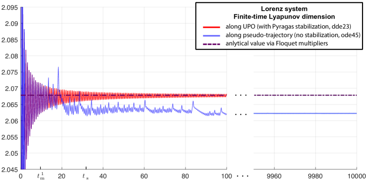
Figure 3: Evolution of FTLDs $\dim_{\rm L}(u(t,\cdot),u^{\rm upo_{1}}_{0})$ (red) and $\dim_{\rm L}(\tilde{u}(t,\cdot),u^{\rm upo_{1}}_{0})$ (blue) computed on the long time interval $t\in[0,10000]$ along the UPO $u^{\rm upo_{1}}(t)=u(t,u^{\rm upo_{1}}_{0})$ (red) and the trajectory $\tilde{u}(t,u^{\rm upo_{1}}_{0})$ (blue) integrated without stabilization, respectively. Both trajectories start from the point $u^{\rm upo_{1}}_{0}=(-6.2262,-11.0027,13.0515)$.

The comparison of the obtained values of finite-time Lyapunov dimensions computed along the stabilized UPO and the trajectory without stabilization gives us the following results. On the initial small part of the time interval, one can indicate the coincidence of these values with a sufficiently high accuracy. For the UPO and for the unstabilized trajectory the finite-time local Lyapunov dimensions $\dim_{\rm L}(u(t,\cdot),u^{\rm upo_{1}}_{0})$ and $\dim_{\rm L}(\tilde{u}(t,\cdot),u^{\rm upo_{1}}_{0})$ coincide up to the 4th decimal place inclusive on the interval $[0,t_{m}^{1}\approx 7\tau_{1}]$. After $t>t_{m}^{1}$ the difference in values becomes significant and the corresponding graphics diverge in such a way that the part of the graph corresponding to the unstabilized trajectory is lower than the part of the graph corresponding to the UPO (see Fig. 2b, Fig. 3).

The Jacobi matrix at the saddle-foci equilibria $S_{\pm}$ has simple eigenvalues, which give the following: $\dim_{\rm L}S_{\pm}=2.0136$. The UPO $u^{\rm upo_{1}}$ with period $\tau_{1}=1.5586$ has the following Floquet multipliers: $\rho_{1}=4.7127$, $\rho_{2}\leavevmode\nobreak\ =\leavevmode\nobreak\ 1$, $\rho_{3}=-1.19\cdot 10^{-10}$ and corresponding Lyapunov exponents: $\{\frac{1}{\tau_{1}}\log\rho_{i}\}_{i=1}^{3}$. Thus, for the local Lyapunov dimension of this UPO we obtain: $\dim_{\rm L}u^{\rm upo_{1}}=2.0678\lessapprox 2.0679=\dim_{\rm L}(u(100,\cdot),u^{\rm upo_{1}}_{0})$.

Using an effective analytical technique, proposed by Leonov (Leonov-1991-Vest, ; Kuznetsov-2016-PLA, ), which is based on a combination of the Douady-Oesterlé approach and the direct Lyapunov method, it is possible to obtain LeonovKKK-2016-CNSCS ; Leonov-2018-UMZh the exact formula of the Lyapunov dimension for the global attractor $\mathcal{A}_{\rm glob}$ of the Lorenz system (1):

$$\dim_{\rm L}\mathcal{A}_{\rm glob}=3-\tfrac{2(\sigma+b+1)}{\sigma+1+\sqrt{(\sigma-1)^{2}+4\sigma r}}$$ (8)

for the case, when $r\sigma>(\sigma+b)(b+1)$.

III Conclusion

In this note, for the Lorenz system (1) with classical values of parameters $r=28$, $\sigma=10$, $b=8/3$ we have studied the Eden conjecture (Eden-1989-PhD, , p.98) and obtained the following relations:

$$\dim_{\rm L}\mathcal{A_{\rm glob}}=\dim_{\rm L}S_{0}=3-\tfrac{2(\sigma+b+1)}{\sigma+1+\sqrt{(\sigma-1)^{2}+4\sigma r}}\!=\!2.4013>$$

$$>\dim_{\rm L}\mathcal{A}\geq\dim_{\rm L}{u}^{\rm upo_{1}}=2.0678>\dim_{\rm L}(\tilde{u}(100,\cdot),u^{\rm upo_{1}}_{0})$$

$$=2.0621>\dim_{\rm L}S_{\pm}=2.0136.$$

Here, since the global Lorenz attractor contains a period-1 UPO: $\mathcal{A}_{\rm glob}\supset u^{\rm upo_{1}}$, we have the following lower-bound estimate for the Lyapunov dimension: $\dim_{\rm L}\mathcal{A}_{\rm glob}\geq 2.0678=\dim_{\rm L}{u}^{\rm upo_{1}}$. Similar experiment and results for the Rössler system (Rossler-1976, ) are presented in KuznetsovM-2019-AIP ; KuznetsovKKMD-2019-IFAC .

Concerning the time of integration, remark that while the time series obtained from a physical experiment are assumed to be reliable on the whole considered time interval, the time series produced by the integration of mathematical dynamical model can be reliable on a limited time interval only due to computational errors (caused by finite precision arithmetic and numerical integration of ODE). Thus, in general, the closeness of the real trajectory $u(t,u_{0})$ and the corresponding pseudo-trajectory $\tilde{u}(t,u_{0})$ calculated numerically can be guaranteed on a limited short time interval only.

In our experiment, if we continue computation over a long time interval $[0,10000]$ of FTLD along the stabilized UPO and the pseudo-trajectory obtained without Pyragas stabilization, as a result, completely different values will be obtained (see Fig. 3). Evolution of $\dim_{\rm L}(u(t,\cdot),u^{\rm upo_{1}}_{0})$ along the stabilized UPO will tend to the analytical value $\dim_{\rm L}{u}^{\rm upo_{1}}=2.0678$, computed via Floquet multipliers, while evolution of $\dim_{\rm L}(\tilde{u}(t,\cdot),u^{\rm upo_{1}}_{0})$ along the pseudo-trajectory will converge to the value $2.0622$. These results are in good agreement with the rigorous analysis of the time interval choices for reliable numerical computation of trajectories for the Lorenz system: the time interval for reliable computation with 16 significant digits and error $10^{-4}$ is estimated as $[0,36]$, with error $10^{-8}$ is estimated as $[0,26]$ (see KehletL-2013 ; KehletL-2017 ), and reliable computation for a longer time interval, e.g. $[0,10000]$ in LiaoW-2014 , is a challenging task that requires significant increase of the precision of the floating-point representation and the use of supercomputers. Analytical aspects of this problem are related to the shadowing theory (see e.g. Pilyugin-2011 ).

References

- (1) E. Lorenz, Deterministic nonperiodic flow, J. Atmos. Sci. 20 (2) (1963) 130–141.
- (2) G. Leonov, N. Kuznetsov, T. Mokaev, Homoclinic orbits, and self-excited and hidden attractors in a Lorenz-like system describing convective fluid motion, The European Physical Journal Special Topics 224 (8) (2015) 1421–1458. doi:10.1140/epjst/e2015-02470-3.
- (3) G. Leonov, N. Kuznetsov, V. Vagaitsev, Localization of hidden Chua’s attractors, Physics Letters A 375 (23) (2011) 2230–2233. doi:10.1016/j.physleta.2011.04.037.
- (4) G. Leonov, N. Kuznetsov, Hidden attractors in dynamical systems. From hidden oscillations in Hilbert-Kolmogorov, Aizerman, and Kalman problems to hidden chaotic attractors in Chua circuits, International Journal of Bifurcation and Chaos in Applied Sciences and Engineering 23 (1), art. no. 1330002. doi:10.1142/S0218127413300024.
- (5) N. Kuznetsov, Hidden attractors in fundamental problems and engineering models. A short survey, Lecture Notes in Electrical Engineering 371 (2016) 13–25, (Plenary lecture at International Conference on Advanced Engineering Theory and Applications 2015). doi:10.1007/978-3-319-27247-4\_2.
- (6) V. Afraımovic, V. Bykov, L. Silnikov, On the origin and structure of the Lorenz attractor 234 (2) (1977) 336–339.
- (7) D. Auerbach, P. Cvitanović, J.-P. Eckmann, G. Gunaratne, I. Procaccia, Exploring chaotic motion through periodic orbits, Physical Review Letters 58 (23) (1987) 2387.
- (8) P. Cvitanović, Periodic orbits as the skeleton of classical and quantum chaos, Physica D: Nonlinear Phenomena 51 (1-3) (1991) 138–151.
- (9) K. Pyragas, Continuous control of chaos by selfcontrolling feedback, Phys. Lett. A. 170 (1992) 421–428.
- (10) N. Kuznetsov, G. Leonov, M. Shumafov, A short survey on Pyragas time-delay feedback stabilization and odd number limitation, IFAC-PapersOnLine 48 (11) (2015) 706–709. doi:10.1016/j.ifacol.2015.09.271.
- (11) G. Chen, X. Yu, On time-delayed feedback control of chaotic systems, IEEE Transactions on Circuits and Systems I: Fundamental Theory and Applications 46 (6) (1999) 767–772.
- (12) J. Lehnert, P. Hövel, V. Flunkert, P. Guzenko, A. Fradkov, E. Schöll, Adaptive tuning of feedback gain in time-delayed feedback control, Chaos: An Interdisciplinary Journal of Nonlinear Science 21 (4) (2011) 043111.
- (13) E. Hooton, A. Amann, Analytical limitation for time-delayed feedback control in autonomous systems, Phys. Rev. Lett. 109 (2012) 154101.
- (14) K. Pyragas, Control of chaos via an unstable delayed feedback controller, Phys. Rev. Lett. 86 (2001) 2265–2268.
- (15) D. Viswanath, The Lindstedt–Poincaré technique as an algorithm for computing periodic orbits, SIAM review 43 (3) (2001) 478–495.
- (16) V. Budanov, Undefined frequencies method, Fundam. Prikl. Mat. 22 (2018) 59–71, (in Russian).
- (17) A. Pchelintsev, A. Polunovskiy, I. Yukhanova, The harmonic balance method for finding approximate periodic solutions of the Lorenz system, Tambov University Reports. Series: Natural and Technical Sciences 24 (2019) 187–203, (in Russian).
- (18) Z. Galias, W. Tucker, Short periodic orbits for the Lorenz system, in: 2008 International Conference on Signals and Electronic Systems, IEEE, 2008, pp. 285–288.
- (19) R. Barrio, A. Dena, W. Tucker, A database of rigorous and high-precision periodic orbits of the Lorenz model, Computer Physics Communications 194 (2015) 76–83.
- (20) C. Grebogi, E. Ott, J. Yorke, Fractal basin boundaries, long-lived chaotic transients, and unstable-unstable pair bifurcation, Physical Review Letters 50 (13) (1983) 935–938.
- (21) G. Leonov, N. Kuznetsov, On differences and similarities in the analysis of Lorenz, Chen, and Lu systems, Applied Mathematics and Computation 256 (2015) 334–343. doi:10.1016/j.amc.2014.12.132.
- (22) G. Chen, N. Kuznetsov, G. Leonov, T. Mokaev, Hidden attractors on one path: Glukhovsky-Dolzhansky, Lorenz, and Rabinovich systems, International Journal of Bifurcation and Chaos in Applied Sciences and Engineering 27 (8), art. num. 1750115.
- (23) J. Sprott, B. Munmuangsaen, Comment on “A hidden chaotic attractor in the classical Lorenz system”, Chaos, Solitons & Fractals 113 (2018) 261–262.
- (24) N. Kuznetsov, The Lyapunov dimension and its estimation via the Leonov method, Physics Letters A 380 (25-26) (2016) 2142–2149. doi:10.1016/j.physleta.2016.04.036.
- (25) N. Kuznetsov, G. Leonov, T. Mokaev, A. Prasad, M. Shrimali, Finite-time Lyapunov dimension and hidden attractor of the Rabinovich system, Nonlinear Dynamics 92 (2) (2018) 267–285. doi:10.1007/s11071-018-4054-z.
- (26) A. Douady, J. Oesterle, Dimension de Hausdorff des attracteurs, C.R. Acad. Sci. Paris, Ser. A. (in French) 290 (24) (1980) 1135–1138.
- (27) G. Leonov, On estimations of Hausdorff dimension of attractors, Vestnik St. Petersburg University: Mathematics 24 (3) (1991) 38–41, [Transl. from Russian: Vestnik Leningradskogo Universiteta. Mathematika, 24(3), 1991, pp. 41-44].
- (28) G. Leonov, N. Kuznetsov, N. Korzhemanova, D. Kusakin, Lyapunov dimension formula for the global attractor of the Lorenz system, Communications in Nonlinear Science and Numerical Simulation 41 (2016) 84–103. doi:10.1016/j.cnsns.2016.04.032.
- (29) G. Leonov, Lyapunov functions in the global analysis of chaotic systems, Ukrainian Mathematical Journal 70 (1) (2018) 42–66.
- (30) A. Eden, An abstract theory of L-exponents with applications to dimension analysis (PhD thesis), Indiana University, 1989.
- (31) O. Rössler, An equation for continuous chaos, Physics Letters A 57 (5) (1976) 397–398.
- (32) N. Kuznetsov, T. Mokaev, Numerical analysis of dynamical systems: unstable periodic orbits, hidden transient chaotic sets, hidden attractors, and finite-time Lyapunov dimension, Journal of Physics: Conference Series 1205 (1), art. num. 012034. doi:10.1088/1742-6596/1205/1/012034.
- (33) N. Kuznetsov, T. Mokaev, E. Kudryashova, O. Kuznetsova, M.-F. Danca, On lower-bound estimates of the Lyapunov dimension and topological entropy for the Rossler systems, 15th IFAC Workshop on Time Delay SystemsAccepted.
- (34) P. Grassberger, I. Procaccia, Measuring the strangeness of strange attractors, Physica D: Nonlinear Phenomena 9 (1-2) (1983) 189–208.
- (35) R. Benzi, G. Paladin, G. Parisi, A. Vulpiani, On the multifractal nature of fully developed turbulence and chaotic systems, Journal of Physics A: Mathematical and General 17 (18) (1984) 3521.
- (36) H. Strogatz, Nonlinear Dynamics and Chaos. With Applications to Physics, Biology, Chemistry, and Engineering, Westview Press, 1994.
- (37) G. Malinetskii, A. Potapov, On calculating the dimension of strange attractors, USSR Computational Mathematics and Mathematical Physics 28 (4) (1988) 39–49.
- (38) J. Sprott, G. Rowlands, Improved correlation dimension calculation, International Journal of Bifurcation and Chaos 11 (07) (2001) 1865–1880.
- (39) A. Fuchs, Nonlinear dynamics in complex systems, Springer, 2013.
- (40) E. Lorenz, The local structure of a chaotic attractor in four dimensions, Physica D: Nonlinear Phenomena 13 (1-2) (1984) 90–104.
- (41) J. Nese, J. Dutton, R. Wells, Calculated attractor dimensions for low-order spectral models, Journal of the atmospheric sciences 44 (15) (1987) 1950–1972.
- (42) C. R. Doering, J. Gibbon, On the shape and dimension of the Lorenz attractor, Dynamics and Stability of Systems 10 (3) (1995) 255–268.
- (43) J. Sprott, Chaos and time-series analysis, Oxford University Press, Oxford, 2003.
- (44) M. Lappa, Thermal convection: patterns, evolution and stability, John Wiley & Sons, 2009.
- (45) J. Sprott, Maximally complex simple attractors, Chaos: An Interdisciplinary Journal of Nonlinear Science 17 (3) (2007) 033124.
- (46) A. Eden, C. Foias, R. Temam, Local and global Lyapunov exponents, Journal of Dynamics and Differential Equations 3 (1) (1991) 133–177, [Preprint No. 8804, The Institute for Applied Mathematics and Scientific Computing, Indiana University, 1988]. doi:10.1007/BF01049491.
- (47) B. Kehlet, A. Logg, Quantifying the computability of the Lorenz system using a posteriori analysis, in: Proceedings of the VI Int. conf. on Adaptive Modeling and Simulation (ADMOS 2013), 2013.
- (48) B. Kehlet, A. Logg, A posteriori error analysis of round-off errors in the numerical solution of ordinary differential equations, Numerical Algorithms 76 (1) (2017) 191–210.
- (49) S. Liao, P. Wang, On the mathematically reliable long-term simulation of chaotic solutions of Lorenz equation in the interval [0,10000], Science China Physics, Mechanics and Astronomy 57 (2) (2014) 330–335.
- (50) S. Pilyugin, Theory of shadowing of pseudotrajectories in dynamical systems, Differencialnie Uravnenia i Protsesy Upravlenia (Differential Equations and Control Processes) 4 (2011) 96–112.