The perils of minimal coupling to electromagnetic field in quantum many-body systems

Abstract

Consistency with the Maxwell equations determines how matter must be coupled to the electromagnetic field (EMF) within the minimal coupling scheme. Specifically, if the Hamiltonian includes just a short-range repulsion among the conduction electrons, as is commonly the case for models of correlated metals, those electrons must be coupled to the full internal EMF, whose longitudinal and transverse components are self-consistently related to the electron charge and current densities through Gauss’s and circuital laws, respectively. Since such self-consistency relation is hard to implement when modelling the non-equilibrium dynamics caused by the EMF, as in pump-probe experiments, it is common to replace in model calculations the internal EMF by the external one. Here we show that such replacement may be extremely dangerous, especially when the frequency of the external EMF is below the intra-band plasma edge.

I Introduction

Modern ultrafast time resolved pump-probe spectroscopy offers the possibility to access the real-time dynamics of a material perturbed by a laser pulse, thus providing information complementary to more traditional experimental techniques. Furthermore, properly tailoring the pump pulse allows ultrafast photoinducing phase transitions into states that may not even exist in thermal equilibrium Ichikawa et al. (2011); Stojchevska et al. (2014). Strongly correlated materials appeared as ideal candidates for such kind of experiments Iwai et al. (2003); Mansart et al. (2010); Lantz et al. (2017); Giannetti et al. (2016); Basov et al. (2017); Lantz et al. (2017); Buzzi et al. (2018); Braun et al. (2018); Singer et al. (2018); Giorgianni et al. (2019), because of their rich phase diagrams that include different insulating and conducting states, often displaying notable properties, such as high-T_c superconductivity Fausti et al. (2011); Dal Conte et al. (2012); Cavalleri (2018).

The experimental activity has, in turn, stimulated a great theoretical effort aimed to interpret the measurements, as well as to achieve control over new states of matter that might be stabilised by a properly designed laser pulse, see for instance Refs. Tsuji et al. (2008, 2011); Aoki et al. (2014); Oka and Kitamura (2019). Evidently, this task requires a proper treatment of the interaction with the electromagnetic field. The minimal coupling scheme, describing the light-matter interaction when only the monopole of the charged particles is taken into account, is explicitly derived in many textbooks Schiff (1968); Mahan (1990) and routinely used to model the electromagnetic field coupling in electronic systems. However, its precise meaning in the case of many-body systems is often largely overlooked, ultimately leading to a possible fallacious description of the effects of light.

In the following we shall show that the inconsiderate use of the simple minimal coupling recipe hides in reality some approximations which are not always justified. In particular we review a correct treatment of the electromagnetic field coupling in a system of electrons within linear regime, pointing out the implicit assumptions which may not be verified in metallic systems. We discuss a simple paradigmatic, yet generic, case in which the difference in the treatment of the external field can lead to rather different results.

II Discussion

We assume a system of charged particles in presence of external sources of the electromagnetic field that can be described in terms of the external scalar, $\phi_{\text{ext}}(\mathbf{r},t)$, and vector potentials, $\boldsymbol{A}_{\text{ext}}(\mathbf{r},t)$. We decompose $\boldsymbol{A}_{\text{ext}}(\mathbf{r},t)=\boldsymbol{A}_{||{\text{ext}}}(\mathbf{r},t)+\boldsymbol{A}_{\perp{\text{ext}}}(\mathbf{r},t)$, where $\boldsymbol{A}_{||{\text{ext}}}(\mathbf{r},t)$ and $\boldsymbol{A}_{\perp{\text{ext}}}(\mathbf{r},t)$ are the longitudinal and transverse components, respectively. In the following we shall work in the Coulomb gauge $\boldsymbol{\nabla}\cdot\boldsymbol{A}_{\text{ext}}(\mathbf{r},t)=0$, so that the vector potential is purely transverse Mahan (1990).

Since our system is made of charged particles, they actually feel “internal” scalar and vector potentials, $\phi(\mathbf{r},t)$ and $\boldsymbol{A}_{\perp}(\mathbf{r},t)$, respectively, which do not in general coincide with the external ones. Because of the linearity of the Maxwell equations, we can express such internal fields as:

$$\phi(\mathbf{r},t) =\phi_{\text{ext}}(\mathbf{r},t)+\phi_{\text{sys}}(\mathbf{r},t)\,,$$ (1)

$$\boldsymbol{A}_{\perp}(\mathbf{r},t) =\boldsymbol{A}_{\perp{\text{ext}}}(\mathbf{r},t)+\boldsymbol{A}_{\perp{\text{sys}}}(\mathbf{r},t)\,,$$

where the system $\phi_{\text{sys}}(\mathbf{r},t)$ and $\boldsymbol{A}_{\perp{\text{sys}}}(\mathbf{r},t)$ potentials are obtained through the Gauss’s law

$$-\nabla^{2}\phi_{\text{sys}}(\mathbf{r},t) =4\pi\,\rho_{\text{sys}}(\mathbf{r},t)\,,$$ (2)

and the circuital law

$$\bigg{(}\frac{\displaystyle\partial^{2}}{\displaystyle\partial t^{2}}-c^{2}\,\nabla^{2}\bigg{)}\,\boldsymbol{A}_{\perp\text{sys}}(\mathbf{r},t) =4\pi\,c\,\boldsymbol{J}_{\perp\text{sys}}(\mathbf{r},t)\,,$$ (3)

with $\rho_{\text{sys}}(\mathbf{r},t)$ the system charge density, and $\boldsymbol{J}_{\perp\text{sys}}(\mathbf{r},t)$ the transverse component of the system current density. Consequently, the internal gauge-invariant electric and magnetic fields are defined in terms of the internal scalar and vector potentials through

$$\boldsymbol{E}_{||}(\mathbf{r},t) =-\boldsymbol{\nabla}\phi(\mathbf{r},t)\,,$$ (4)

$$\boldsymbol{E}_{\perp}(\mathbf{r},t) =-\frac{1}{c}\,\frac{\displaystyle\partial\boldsymbol{A}_{\perp}(\mathbf{r},t)}{\displaystyle\partial t}\,,$$

$$\boldsymbol{B}_{\perp}(\mathbf{r},t) =\boldsymbol{\nabla}\wedge\boldsymbol{A}_{\perp}(\mathbf{r},t)\,.$$

Using the above definitions, the Hamiltonian that describes our system coupled to the electromagnetic field, which we assume to be classical, reads, in the minimal coupling scheme Schiff (1968); Mahan (1990) and neglecting the Zeeman term,

$$\mathcal{H} =\int d\mathbf{r}\,\Bigg{\{}\Bigg{[}\sum_{\sigma}\,\Psi^{\dagger}_{\sigma}(\mathbf{r})\,\frac{\displaystyle 1}{\displaystyle 2m}\bigg{(}-i\hbar\,\boldsymbol{\nabla}+\frac{\displaystyle e}{\displaystyle c}\,\boldsymbol{A}(\mathbf{r},t)\bigg{)}^{2}\,\Psi^{\phantom{\dagger}}_{\sigma}(\mathbf{r})\,\Bigg{]}+V(\mathbf{r})\,\Psi^{\dagger}_{\sigma}(\mathbf{r})\,\Psi^{\phantom{\dagger}}_{\sigma}(\mathbf{r})\,\Bigg{\}}$$ (5)

$$\qquad+\frac{\displaystyle e^{2}}{\displaystyle 2}\,\sum_{\sigma\sigma^{\prime}}\int d\mathbf{r}\,d\mathbf{r}^{\prime}\,\Psi_{\sigma}^{\dagger}(\mathbf{r})\,\Psi_{\sigma^{\prime}}^{\dagger}(\mathbf{r}^{\prime})\;\frac{\displaystyle 1}{\displaystyle\;\big{|}\mathbf{r}-\mathbf{r}^{\prime}\big{|}\;}\;\Psi_{\sigma^{\prime}}^{\phantom{\dagger}}(\mathbf{r}^{\prime})\,\Psi_{\sigma}^{\phantom{\dagger}}(\mathbf{r})+\int d\mathbf{r}\,\phi_{\text{ext}}(\mathbf{r},t)\,\rho(\mathbf{r},t)\,,$$

where $\Psi^{\phantom{\dagger}}_{\sigma}(\mathbf{r})$ is the Fermi field of spin $\sigma$ electrons, $V(\mathbf{r})$ the periodic potential of an underlying lattice of immobile ions that also provide a positive charge density, $\rho_{\text{ion}}(\mathbf{r})$, neutralising the electron one. Thus we have: $\rho(\mathbf{r})\equiv\rho_{\text{ion}}(\mathbf{r})-e\,\sum_{\sigma}\Psi_{\sigma}^{\dagger}(\mathbf{r})\,\Psi_{\sigma}^{\phantom{\dagger}}(\mathbf{r})$.

It is worth emphasising that Eqs. (2) and (3), where

$$\rho_{\text{sys}}(\mathbf{r},t) =\langle\,\rho(\mathbf{r})\,\rangle\,,$$ (6)

$$\boldsymbol{J}_{\perp\text{sys}}(\mathbf{r},t) =-c\,\big{\langle}\;\frac{\displaystyle\delta\mathcal{H}}{\displaystyle\delta\boldsymbol{A}_{\perp}(\mathbf{r},t)}\;\big{\rangle}\,,$$

to be verified require that

1. one must explicitly include the Coulomb interaction among the electrons in order for the Hamiltonian (5) to involve only the external longitudinal field $\phi_{\text{ext}}(\mathbf{r},t)$;

2. the transverse vector potential $\boldsymbol{A}_{\perp}(\mathbf{r},t)$ is the internal one, i.e., the sum of the external potential $\boldsymbol{A}_{\perp\text{ext}}(\mathbf{r},t)$ plus the one generated by the electrons, $\boldsymbol{A}_{\perp\text{sys}}(\mathbf{r},t)$, through Eq. (3).

The issue is that both points 1. and 2. make it difficult modelling the system dynamics during and after the action of an electromagnetic pulse. To proceed further, some approximations have to be assumed. Concerning point 1., we note that correlated materials are commonly described in terms of lattice models with short range electron-electron interactions, e.g., the paradigmatic Hubbard model. Although such models are in general not exactly solvable, powerful techniques are available to investigate them in controlled approximation schemes, such as dynamical mean field theory (DMFT)Georges et al. (1996), originally designed to treat just short range interaction. Several attempts to add non-local correlations in equilibrium DMFT have been put forward Biermann (2014); Werner and Casula (2016); Rohringer et al. (2018), still the inclusion of the true long-range Coulomb interaction remains a serious challenge. The extension of some of those attempts to the out-of-equilibrium regime has been achieved in simple casesAoki et al. (2014); Golez et al. (2017, 2019), but a more systematic development and a proper description of the dynamics in presence of a longitudinal field is yet to come.

However, since the laser frequency in experiments usually ranges from far to near infrared, i.e. wavelengths $\lambda\geq 1\mu\text{m}$, the difference between longitudinal and transverse components of the electromagnetic field is negligible. In this case, one can in principle focus only on the transverse response, which is seemingly less sensitive to the long range tail of the Coulomb repulsion irr .

However, the long range nature of the coupling to the transverse field is hidden in point 2. above, which entails the self-consistency condition (3) that is not easy to implement in an actual calculation. One can avoid that self-consistency by treating the transverse field quantum mechanically, and integrating out the photons. The result would be that only the external vector potential would now appear in the minimal coupling scheme, at the cost of introducing a current-current interaction among the electrons, non-local both in time and space. At the end, one faces again the same problems as in the longitudinal response, worsened by the non-locality in time.

In view of the above difficulties, it is rather common to simply ignore points 1. and 2. above, and just consider models of correlated electrons interacting via a short range repulsion, and minimally coupled to a uniform vector potential assumed to coincide with the external one, $\boldsymbol{A}(t)=\boldsymbol{A}_{\text{ext}}(t)$, see, for example, Refs. Aoki et al. (2014) and Oka and Kitamura (2019).

Our aim here is not to revise all results that have been so far obtained under those simplifications, but just to select few examples that can be explicitly worked out and where the difference between taking or not into account points 1. and 2. is most dramatic.

For simplicity, we consider the half-filled single-band Hubbard model in a three dimensional cubic lattice with nearest neighbour hopping $-\mathsf{t}$, and in the presence of a uniform AC vector potential. Using the Peierls substitution method, the Hamiltonian reads

$$\mathcal{H}(t) =\sum_{\mathbf{k}\sigma}\,\varepsilon\Big{(}\mathbf{k}+\frac{\displaystyle e}{\displaystyle\hbar c}\,\boldsymbol{A}(t)\Big{)}\,c^{\dagger}_{\mathbf{k}\sigma}\,c^{\phantom{\dagger}}_{\mathbf{k}\sigma}$$ (7)

$$\qquad+\frac{\displaystyle 1}{\displaystyle 2}\,\sum_{i,j}\,\big{(}n_{i}-1\big{)}\,U_{ij}\,\big{(}n_{j}-1\big{)}$$

$$=\mathcal{H}_{0}+\sum_{\mathbf{k}\sigma}\,\bigg{(}\varepsilon\Big{(}\mathbf{k}+\frac{\displaystyle e}{\displaystyle\hbar c}\,\boldsymbol{A}(t)\Big{)}-\epsilon(\mathbf{k})\bigg{)}\,c^{\dagger}_{\mathbf{k}\sigma}\,c^{\phantom{\dagger}}_{\mathbf{k}\sigma}$$

$$=\mathcal{H}_{0}+\delta\mathcal{H}(t)\,,$$

where

$$\varepsilon(\mathbf{k}) =-2\mathsf{t}\,\sum_{n=1}^{3}\,\cos k_{n}a\,,$$ (8)

with $a$ the lattice constant, $\boldsymbol{A}(t)$ the internal vector potential, transverse and longitudinal loosing their meaning in the present uniform case, and $U_{ij}$ the Coulomb interaction.

Focusing on the response to the internal $\boldsymbol{A}(t)$, we can sensibly discard the long-range tail of $U_{ij}$ irr , and thus approximate $U_{ij}=U$ if $i=j$, and zero otherwise, i.e., the standard local Hubbard repulsion.

We assume to be in a linear response regime, and that the probing measurement is performed well beyond the characteristic relaxation time of the system Perfetti et al. (2008); Novelli et al. (2014); Wall et al. (2018). With those assumptions the Hamiltonian is

$$\mathcal{H}(t) \simeq\sum_{\mathbf{k}\sigma}\,\Bigg{(}\varepsilon(\mathbf{k})\bigg{(}1-\frac{\displaystyle e^{2}a^{2}}{\displaystyle\,6\hbar^{2}c^{2}\,}\;\boldsymbol{A}(t)\cdot\boldsymbol{A}(t)\bigg{)}+\frac{\displaystyle e}{\displaystyle\hbar c}\;\frac{\displaystyle\partial\varepsilon(\mathbf{k})}{\displaystyle\partial\mathbf{k}}\cdot\boldsymbol{A}(t)\Bigg{)}\,c^{\dagger}_{\mathbf{k}\sigma}\,c^{\phantom{\dagger}}_{\mathbf{k}\sigma}+\frac{\displaystyle U}{\displaystyle 2}\,\sum_{i}\,\big{(}n_{i}-1\big{)}^{2}\,,$$ (9)

and the equation relating the internal field to the external one has the simple solution, in the frequency space,

$$\boldsymbol{A}(\omega) =\frac{\displaystyle\boldsymbol{A}_{\text{ext}}(\omega)}{\displaystyle\epsilon(\omega)}\;,$$ (10)

with the uniform dielectric constant

$$\epsilon(\omega) =1+i\,\frac{\displaystyle 4\pi}{\displaystyle\omega}\;\sigma(\omega)\,,$$ (11)

where $\sigma(\omega)$ is the optical conductivity that, in linear response, is defined by

$$\boldsymbol{J}_{\text{sys}}(\omega) =\sigma(\omega)\,\boldsymbol{E}(\omega)=\frac{\displaystyle i\omega}{\displaystyle c}\;\sigma(\omega)\,\boldsymbol{A}(\omega)\,,$$ (12)

and can be calculated through the current-current response function. We shall here focus on two physical quantities that can be readily obtained once the optical conductivity and the dielectric constant are known.

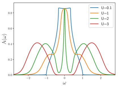
Figure 1: (Color online) Evolution of the local spectral function $A(\omega)$ of the single-band Hubbard model on the cubic lattice. Data are for different values of $U=0.1$, $1$ ,$2$, $3$, from the weakly correlated metal up to the Mott insulator.

The first is the expectation value of the hopping

$$T\big{(}\boldsymbol{A}(t)\big{)} =\big{\langle}\;\frac{\displaystyle\partial\mathcal{H}(t)}{\displaystyle\partial\mathsf{t}}\;\big{\rangle}$$ (13)

$$\simeq T(0)\,\bigg{(}1-\frac{\displaystyle e^{2}a^{2}}{\displaystyle\,6\hbar^{2}c^{2}\,}\;\boldsymbol{A}(t)\cdot\boldsymbol{A}(t)\bigg{)}\,,$$

which is renormalised downwards by the electromagnetic field, with potentially interesting consequences, see, e.g., Tsuji et al. (2011, 2008); Ono et al. (2017). We choose to quantify this reduction through the relative variation of the hopping expectation value averaged over one period $\tau=2\pi/\omega$ of a monochromatic field of frequency $\omega$, which reads

$$\frac{\displaystyle\delta T}{\displaystyle T} = \int_{0}^{\tau}\frac{\displaystyle dt}{\displaystyle\tau}\;\left|\frac{\displaystyle\;T\big{(}\boldsymbol{A}(t)\big{)}-T(0)\;}{\displaystyle T(0)}\right|=\frac{\displaystyle e^{2}a^{2}}{\displaystyle\,12\hbar^{2}\omega^{2}\,}\;\big{|}\boldsymbol{E}(\omega)\big{|}^{2}$$ (14)

$$= \frac{\displaystyle e^{2}a^{2}}{\displaystyle\,12\hbar^{2}\omega^{2}\,}\;\frac{\displaystyle\;\big{|}\boldsymbol{E}_{\text{ext}}(\omega)\big{|}^{2}\;}{\displaystyle\big{|}\epsilon(\omega)\big{|}^{2}}\;.$$

The reduction thus becomes significant when $\delta T/T=1$, which corresponds to a threshold field

$$\big{|}\boldsymbol{E}^{\text{th}}_{\text{ext}}(\omega)\big{|}=\frac{\displaystyle\sqrt{12}\,\hbar\omega}{\displaystyle ea}\,\big{|}\epsilon(\omega)\big{|}\,.$$ (15)

We observe that, if one discards point 2., i.e., assumes $\boldsymbol{A}(t)$ to coincide with $\boldsymbol{A}_{\text{ext}}(t)$, the threshold field changes into $\big{|}\boldsymbol{E}^{\text{th}}_{\text{ext}}(\omega)\big{|}_{\text{appx}}$ related to the true one of Eq. (15) through

$$\frac{\displaystyle\;\big{|}\boldsymbol{E}^{\text{th}}_{\text{ext}}(\omega)\big{|}_{\text{appx}}\;}{\displaystyle\big{|}\boldsymbol{E}^{\text{th}}_{\text{ext}}(\omega)\big{|}}=\frac{\displaystyle 1}{\displaystyle\;\big{|}\epsilon(\omega)\big{|}\;}\equiv Y_{1}(\omega)\,.$$ (16)

We shall use $Y_{1}(\omega)$ as first estimate of the error one can do by replacing the internal vector potential with the external one in the minimal coupling scheme (5).

The other physical quantity we consider is the power dissipated by the monochromatic electromagnetic field during one period, defined as, see Eq. (7),

$$P(\omega) =\int_{0}^{\tau}\frac{\displaystyle dt}{\displaystyle\tau}\;\frac{\displaystyle\partial}{\displaystyle\partial t}\,\langle\;\mathcal{H}_{0}\;\rangle=-i\,\int_{0}^{\tau}\frac{\displaystyle dt}{\displaystyle\tau}\;\langle\;\Big{[}\mathcal{H}_{0}\,,\,\mathcal{H}(t)\Big{]}\;\rangle$$ (17)

$$=\frac{\displaystyle 1}{\displaystyle 2}\,\text{Re}\,\sigma(\omega)\;\big{|}\boldsymbol{E}(\omega)\big{|}^{2}=\frac{\displaystyle 1}{\displaystyle 2}\,\frac{\displaystyle\;\text{Re}\,\sigma(\omega)\;}{\displaystyle\;\big{|}\epsilon(\omega)\big{|}^{2}\;}\;\big{|}\boldsymbol{E}_{\text{ext}}(\omega)\big{|}^{2}\,.$$

As before, if one uses $\boldsymbol{A}_{\text{ext}}(t)$ instead of $\boldsymbol{A}(t)$ in the Hamiltonian, the power dissipated takes the approximate expression

$$P_{\text{appx}}(\omega) =\frac{\displaystyle 1}{\displaystyle 2}\,\text{Re}\,\sigma(\omega)\;\big{|}\boldsymbol{E}_{\text{ext}}(\omega)\big{|}^{2}\,.$$ (18)

$P(\omega)$ is the energy of the electromagnetic field that is actually absorbed by the system per unit time. If the system thermalises, such supplied energy is transformed into heat that yields an effective temperature raise $\Delta T$ given by

$$\Delta T =\frac{\displaystyle P(\omega)\,\tau_{\text{pulse}}}{\displaystyle c_{V}}\;,$$ (19)

where $\tau_{\text{pulse}}$ is the laser pulse duration, and $c_{V}$ the system specific heat. Seemingly, if one identifies the vector potential in the minimal coupling with the external one, and thus uses the approximate expression (18), the temperature raise changes into $\Delta T_{\text{appx}}$, where

$$\frac{\displaystyle\Delta T_{\text{appx}}}{\displaystyle\Delta T} =\frac{\displaystyle P_{\text{appx}}(\omega)}{\displaystyle P(\omega)}=\big{|}\epsilon(\omega)\big{|}^{2}\equiv Y_{2}(\omega)\,.$$ (20)

$Y_{2}(\omega)$ is the other quantity, besides $Y_{1}(\omega)$ of Eq. (16), that we shall study to evaluate how wrong the replacement of $\boldsymbol{A}(t)$ by $\boldsymbol{A}_{\text{ext}}(t)$ in the minimal coupling scheme may be.

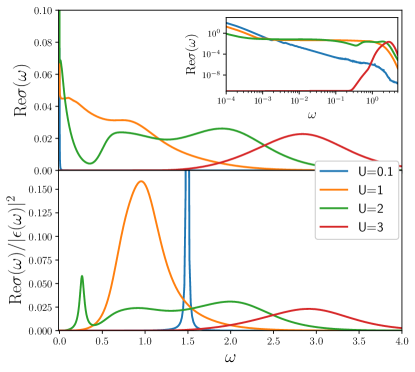
Figure 2: (Color online) Top panel: absorption spectrum from the internal field as obtained from the optical conductivity. Inset: low energy behavior in logarithmic scale. Bottom panel: absorption spectrum from the external field. See main text for the defintion

III Results

We calculate at zero temperature the optical properties of the Hubbard Hamiltonian (9) at half-filling by means of DMFT Georges et al. (1996), using numerical renormalisation group (NRG) as impurity solver Hewson (1993); Bulla et al. (1998, 2008). Specifically, we calculate the single-particle Green’s function, through which we obtain the local single-particle spectral function, $A(\omega)$, and the uniform current-current response function Georges et al. (1996); Rozenberg et al. (1995); Tomczak and Biermann (2009); Arsenault and Tremblay (2013); Zitko et al. (2015), which, in turn, allows computing the optical conductivity and thus the dielectric constant. In what follows we shall use as units of measurement the half-bandwidth $8\mathsf{t}=1$, the lattice constant $a=1$, the electric charge $e=1$ and finally $\hbar=1$.

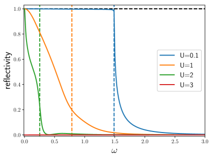
Figure 3: (Color online) Reflectivity as function of frequency. Data are for the same values of $U$ of previous figures. The vertical lines indicate the positions of the intra-band plasmons. Note that the $U=3$ Mott insulator case is nearly vanishing.

To fix ideas, we show in Fig. 1 the evolution of the local single-particle spectral functions $A(\omega)$ with increasing $U$ from the weakly correlated metal, $U=0.1$, up to the Mott insulator, $U=3$. We note that for the intermediate interaction strength ($U=2$) coherent quasiparticles narrowly peaked at the chemical potential $\omega=0$ coexist with the lower and upper forming Hubbard sidebands, centred at $\omega\sim\pm U/2$, respectively.

We now discuss the optical properties of the model from the weak coupling metal to the Mott insulator Rozenberg et al. (1995); Georges et al. (1996); Limelette et al. (2003); Comanac et al. (2008). According to Eq. (17), the absorption spectrum from the internal field is the real part of the optical conductivity, $\text{Re}\,\sigma(\omega)$, while that from the external field is instead $\text{Re}\,\sigma(\omega)/|\epsilon(\omega)|^{2}$, shown, respectively, in the top and bottom panels of Fig. 2.

Looking at the top panel of Fig. 2, we observe that the optical conductivity of the weakly correlated metal at $U=0.1$ just shows a very narrow Drude peak. This peak broadens upon increasing the interaction strength $U$. Two additional absorption peaks emerge, which are most visible for $U=2$: an intermediate one involving an excitation from/to the quasiparticle peak to/from the Hubbard bands, and a high-energy peak corresponding to an excitation between the two Hubbard bands. The latter is the only one that survives in the Mott insulator at $U=3$.

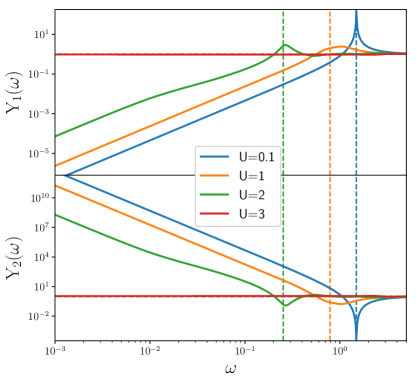
Figure 4: (Color online) The behavior of the functions $Y_{1}(\omega)$ (top panel), Eq. (16), and $Y_{2}(\omega)$ (bottom panel), Eq. (20). Data are for the same values of $U$ as in previous figures. The vertical lines indicate the roots of the real-part of the dielectric constant.

The absorption spectrum from the external field

$$\frac{\displaystyle\text{Re}\,\sigma(\omega)}{\displaystyle\,\big{|}\epsilon(\omega)\big{|}^{2}\,}=-\frac{\displaystyle\omega}{\displaystyle 4\pi}\;\text{Im}\bigg{(}\frac{\displaystyle 1}{\displaystyle\epsilon(\omega)}\bigg{)}\,,$$ (21)

is presented in the bottom panel of Fig. 2. This quantity is rather different from the internal field absorption spectrum, being dominated by the plasmon modes, i.e., the peaks of $\text{Im}(-1/\epsilon(\omega))$. At weak coupling, $U=0.1$, there is just a single and very sharp intra-band plasmon. The plasmon peak shifts to lower frequencies upon increasing $U$. Meanwhile, additional inter-band, i.e., involving the Hubbard sidebands, broad plasma modes emerge, see the intermediate coupling case at $U=2$. In Fig. 3 we show the corresponding reflectivity, where the plasma edges become clearly visible.

We can now return to our original aim, and try to quantify through the behavior of the quantities $Y_{1}(\omega)$ in Eq. (16) and $Y_{2}(\omega)$ in Eq. (20) the error generated by using the external vector potential in place of the internal one within the minimal coupling scheme. We show the functions $Y_{1}(\omega)$ and $Y_{2}(\omega)$ in Fig. 4. From the behaviour of $Y_{1}(\omega)$, top panel of Fig. 4, we conclude that, in the metal phase and for frequencies smaller than the intra-band plasmon modes, defined by the roots of $\text{Re}(\epsilon(\omega))$, the external field required to significantly reduce the expectation value of the hopping is orders of magnitude larger than what is predicted by assuming that $\boldsymbol{A}(t)$ in the Hamiltonian (5) can be replaced by the external field $\boldsymbol{A}_{\text{ext}}(t)$. Within that same assumption and in the same range of frequencies, the temperature raise produced by the field would be huge compared to the actual value, see bottom panel in Fig. 4. On the contrary, and not surprisingly, $\boldsymbol{A}(t)\simeq\boldsymbol{A}_{\text{ext}}(t)$ works well in the insulating phase at $U=3$.

In conclusion, we have shown that replacing in the minimal coupling scheme the internal vector potential, which is self-consistently determined by the system charges, by the external vector potential may be quite dangerous, in particular in a metal and when the frequency of light is small compared with the intra-band plasma edge, which is where screening effects are maximal. In correlated metals the precise value of such plasma edge, which originates from the itinerant carriers and is proportional to the square root of their contribution to the optical sum rule Millis et al. (2005); Qazilbash et al. (2009); Degiorgi (2011), is material dependent Bozovic (1990); Degiorgi et al. (1994); Qazilbash et al. (2009); Basov et al. (2011) and typically ranges from mid to near infrared. This in turn implies that in common pump-probe experiments the internal field $\boldsymbol{A}(t)$ is rather different from the external one $\boldsymbol{A}_{\text{ext}}(t)$, hence replacing the former by the latter in model calculations is simply incorrect.

We end mentioning that mixing up the response to the internal field with that to the external one is a mistake that tends to recur. It was, e.g., at the origin of early claims that the conductance of Luttinger liquids is renormalised by interaction; a wrong statement corrected in Oreg and Finkel’stein (1996) by similar arguments as ours.

We acknowledge support by the European Research Council (ERC) under H2020 Advanced Grant No. 692670 “FIRSTORM”.

References

- Ichikawa et al. (2011) H. Ichikawa, S. Nozawa, T. Sato, A. Tomita, K. Ichiyanagi, M. Chollet, L. Guerin, N. Dean, A. Cavalleri, S.-i. Adachi, et al., Nature Materials 10, 101 (2011), URL https://doi.org/10.1038/nmat2929.
- Stojchevska et al. (2014) L. Stojchevska, I. Vaskivskyi, T. Mertelj, P. Kusar, D. Svetin, S. Brazovskii, and D. Mihailovic, Science 344, 177 (2014), ISSN 0036-8075, eprint https://science.sciencemag.org/content/344/6180/177.full.pdf, URL https://science.sciencemag.org/content/344/6180/177.
- Iwai et al. (2003) S. Iwai, M. Ono, A. Maeda, H. Matsuzaki, H. Kishida, H. Okamoto, and Y. Tokura, Phys. Rev. Lett. 91, 057401 (2003), URL https://link.aps.org/doi/10.1103/PhysRevLett.91.057401.
- Mansart et al. (2010) B. Mansart, D. Boschetto, S. Sauvage, A. Rousse, and M. Marsi, EPL (Europhysics Letters) 92, 37007 (2010), URL https://doi.org/10.1209%2F0295-5075%2F92%2F37007.
- Lantz et al. (2017) G. Lantz, B. Mansart, D. Grieger, D. Boschetto, N. Nilforoushan, E. Papalazarou, N. Moisan, L. Perfetti, V. L. R. Jacques, D. Le Bolloc’h, et al., Nature Communications 8, 13917 (2017), URL https://doi.org/10.1038/ncomms13917.
- Giannetti et al. (2016) C. Giannetti, M. Capone, D. Fausti, M. Fabrizio, F. Parmigiani, and D. Mihailovic, Advances in Physics 65, 58 (2016), eprint https://doi.org/10.1080/00018732.2016.1194044, URL https://doi.org/10.1080/00018732.2016.1194044.
- Basov et al. (2017) D. N. Basov, R. D. Averitt, and D. Hsieh, Nature Materials 16, 1077 EP (2017), URL https://doi.org/10.1038/nmat5017.
- Buzzi et al. (2018) M. Buzzi, M. Först, R. Mankowsky, and A. Cavalleri, Nature Reviews Materials 3, 299 (2018), URL https://doi.org/10.1038/s41578-018-0024-9.
- Braun et al. (2018) J. M. Braun, H. Schneider, M. Helm, R. Mirek, L. A. Boatner, R. E. Marvel, R. F. Haglund, and A. Pashkin, New Journal of Physics 20, 083003 (2018), URL https://doi.org/10.1088%2F1367-2630%2Faad4ef.
- Singer et al. (2018) A. Singer, J. G. Ramirez, I. Valmianski, D. Cela, N. Hua, R. Kukreja, J. Wingert, O. Kovalchuk, J. M. Glownia, M. Sikorski, et al., Phys. Rev. Lett. 120, 207601 (2018), URL https://link.aps.org/doi/10.1103/PhysRevLett.120.207601.
- Giorgianni et al. (2019) F. Giorgianni, J. Sakai, and S. Lupi, Nature Communications 10, 1159 (2019), URL https://doi.org/10.1038/s41467-019-09137-6.
- Fausti et al. (2011) D. Fausti, R. I. Tobey, N. Dean, S. Kaiser, A. Dienst, M. C. Hoffmann, S. Pyon, T. Takayama, H. Takagi, and A. Cavalleri, Science 331, 189 (2011), ISSN 0036-8075, eprint https://science.sciencemag.org/content/331/6014/189.full.pdf, URL https://science.sciencemag.org/content/331/6014/189.
- Dal Conte et al. (2012) S. Dal Conte, C. Giannetti, G. Coslovich, F. Cilento, D. Bossini, T. Abebaw, F. Banfi, G. Ferrini, H. Eisaki, M. Greven, et al., Science 335, 1600 (2012), URL http://science.sciencemag.org/content/335/6076/1600.abstract.
- Cavalleri (2018) A. Cavalleri, Contemporary Physics 59, 31 (2018), eprint https://doi.org/10.1080/00107514.2017.1406623, URL https://doi.org/10.1080/00107514.2017.1406623.
- Tsuji et al. (2008) N. Tsuji, T. Oka, and H. Aoki, Phys. Rev. B 78, 235124 (2008), URL https://link.aps.org/doi/10.1103/PhysRevB.78.235124.
- Tsuji et al. (2011) N. Tsuji, T. Oka, P. Werner, and H. Aoki, Phys. Rev. Lett. 106, 236401 (2011), URL https://link.aps.org/doi/10.1103/PhysRevLett.106.236401.
- Aoki et al. (2014) H. Aoki, N. Tsuji, M. Eckstein, M. Kollar, T. Oka, and P. Werner, Rev. Mod. Phys. 86, 779 (2014), URL https://link.aps.org/doi/10.1103/RevModPhys.86.779.
- Oka and Kitamura (2019) T. Oka and S. Kitamura, Annual Review of Condensed Matter Physics 10, 387 (2019), eprint https://doi.org/10.1146/annurev-conmatphys-031218-013423, URL https://doi.org/10.1146/annurev-conmatphys-031218-013423.
- Schiff (1968) L. I. Schiff, Quantum Mechanics (McGraw-Hill, New York, 1968).
- Mahan (1990) G. D. Mahan, Many-Particle Physics (Springer US, 1990), chapter 1, section B.
- Georges et al. (1996) A. Georges, G. Kotliar, W. Krauth, and M. J. Rozenberg, Rev. Mod. Phys. 68, 13 (1996).
- Biermann (2014) S. Biermann, Journal of Physics: Condensed Matter 26, 173202 (2014), URL https://doi.org/10.1088%2F0953-8984%2F26%2F17%2F173202.
- Werner and Casula (2016) P. Werner and M. Casula, Journal of Physics: Condensed Matter 28, 383001 (2016), URL https://doi.org/10.1088%2F0953-8984%2F28%2F38%2F383001.
- Rohringer et al. (2018) G. Rohringer, H. Hafermann, A. Toschi, A. A. Katanin, A. E. Antipov, M. I. Katsnelson, A. I. Lichtenstein, A. N. Rubtsov, and K. Held, Rev. Mod. Phys. 90, 025003 (2018), URL https://link.aps.org/doi/10.1103/RevModPhys.90.025003.
- Golez et al. (2017) D. Golez, L. Boehnke, H. U. R. Strand, M. Eckstein, and P. Werner, Phys. Rev. Lett. 118, 246402 (2017), URL https://link.aps.org/doi/10.1103/PhysRevLett.118.246402.
- Golez et al. (2019) D. Golez, L. Boehnke, M. Eckstein, and P. Werner, Phys. Rev. B 100, 041111 (2019), URL https://link.aps.org/doi/10.1103/PhysRevB.100.041111.
- (27) For instance, the Feynman diagram expansion of the transverse response lacks diagrams that are reducible by cutting an interaction line, and which are singular in the long wavelength limit. The same diagrams must not be taken into account also in the case one studies directly the response to the internal field, either transverse or longitudinal. In both cases, restricting the perturbation series just to the diagrams irreducible to cutting an interaction line, one would not find qualitative differences between a long-range interaction and a short-range one.
- Perfetti et al. (2008) L. Perfetti, P. A. Loukakos, M. Lisowski, U. Bovensiepen, M. Wolf, H. Berger, S. Biermann, and A. Georges, New Journal of Physics 10, 053019 (2008), URL https://doi.org/10.1088%2F1367-2630%2F10%2F5%2F053019.
- Novelli et al. (2014) F. Novelli, G. De Filippis, V. Cataudella, M. Esposito, I. Vergara, F. Cilento, E. Sindici, A. Amaricci, C. Giannetti, D. Prabhakaran, et al., Nature Communications 5, 5112 (2014), URL https://doi.org/10.1038/ncomms6112.
- Wall et al. (2018) S. Wall, S. Yang, L. Vidas, M. Chollet, J. M. Glownia, M. Kozina, T. Katayama, T. Henighan, M. Jiang, T. A. Miller, et al., Science 362, 572 (2018), ISSN 0036-8075, eprint https://science.sciencemag.org/content/362/6414/572.full.pdf, URL https://science.sciencemag.org/content/362/6414/572.
- Ono et al. (2017) A. Ono, H. Hashimoto, and S. Ishihara, Phys. Rev. B 95, 085123 (2017), URL https://link.aps.org/doi/10.1103/PhysRevB.95.085123.
- Hewson (1993) A. Hewson, The Kondo Problem to Heavy Fermions (Cambridge University Press, New York, N.Y., 1993).
- Bulla et al. (1998) R. Bulla, A. C. Hewson, and T. Pruschke, Journal of Physics: Condensed Matter 10, 8365 (1998), URL https://doi.org/10.1088%2F0953-8984%2F10%2F37%2F021.
- Bulla et al. (2008) R. Bulla, T. A. Costi, and T. Pruschke, Rev. Mod. Phys. 80, 395 (2008), URL https://link.aps.org/doi/10.1103/RevModPhys.80.395.
- Rozenberg et al. (1995) M. J. Rozenberg, G. Kotliar, H. Kajueter, G. A. Thomas, D. H. Rapkine, J. M. Honig, and P. Metcalf, Phys. Rev. Lett. 75, 105 (1995), URL https://link.aps.org/doi/10.1103/PhysRevLett.75.105.
- Tomczak and Biermann (2009) J. M. Tomczak and S. Biermann, Phys. Rev. B 80, 085117 (2009), URL https://link.aps.org/doi/10.1103/PhysRevB.80.085117.
- Arsenault and Tremblay (2013) L.-F. m. c. Arsenault and A.-M. S. Tremblay, Phys. Rev. B 88, 205109 (2013), URL https://link.aps.org/doi/10.1103/PhysRevB.88.205109.
- Zitko et al. (2015) R. Zitko, i. c. v. Osolin, and P. Jeglič, Phys. Rev. B 91, 155111 (2015), URL https://link.aps.org/doi/10.1103/PhysRevB.91.155111.
- Limelette et al. (2003) P. Limelette, A. Georges, D. Jérome, P. Wzietek, P. Metcalf, and J. M. Honig, Science 302, 89 (2003), ISSN 0036-8075, eprint https://science.sciencemag.org/content/302/5642/89.full.pdf, URL https://science.sciencemag.org/content/302/5642/89.
- Comanac et al. (2008) A. Comanac, L. de’Medici, M. Capone, and A. J. Millis, Nature Physics 4, 287 (2008), URL https://doi.org/10.1038/nphys883.
- Millis et al. (2005) A. J. Millis, A. Zimmers, R. P. S. M. Lobo, N. Bontemps, and C. C. Homes, Phys. Rev. B 72, 224517 (2005), URL https://link.aps.org/doi/10.1103/PhysRevB.72.224517.
- Qazilbash et al. (2009) M. M. Qazilbash, J. J. Hamlin, R. E. Baumbach, L. Zhang, D. J. Singh, M. B. Maple, and D. N. Basov, Nature Physics 5, 647 (2009), URL https://doi.org/10.1038/nphys1343.
- Degiorgi (2011) L. Degiorgi, New Journal of Physics 13, 023011 (2011), URL https://doi.org/10.1088%2F1367-2630%2F13%2F2%2F023011.
- Bozovic (1990) I. Bozovic, Phys. Rev. B 42, 1969 (1990), URL https://link.aps.org/doi/10.1103/PhysRevB.42.1969.
- Degiorgi et al. (1994) L. Degiorgi, E. J. Nicol, O. Klein, G. Grüner, P. Wachter, S.-M. Huang, J. Wiley, and R. B. Kaner, Phys. Rev. B 49, 7012 (1994), URL http://link.aps.org/doi/10.1103/PhysRevB.49.7012.
- Basov et al. (2011) D. N. Basov, R. D. Averitt, D. van der Marel, M. Dressel, and K. Haule, Rev. Mod. Phys. 83, 471 (2011), URL https://link.aps.org/doi/10.1103/RevModPhys.83.471.
- Oreg and Finkel’stein (1996) Y. Oreg and A. M. Finkel’stein, Phys. Rev. B 54, R14265 (1996), URL https://link.aps.org/doi/10.1103/PhysRevB.54.R14265.