©2020 IEEE. Personal use of this material is permitted. Permission from IEEE must be obtained for all other uses, in any current or future media, including reprinting/republishing this material for advertising or promotional purposes, creating new collective works, for resale or redistribution to servers or lists, or reuse of any copyrighted component of this work in other works.

S-DIGing: A Stochastic Gradient Tracking Algorithm for Distributed Optimization

Huaqing Li , Lifeng Zheng, Zheng Wang, Yu Yan, Liping Feng, and Jing Guo The work described in this paper is supported in part by the National Natural Science Foundation of China under Grant 61773321, in part by the Innovation Support Program for Chongqing Overseas Returnees under Grant cx2017043, and in part by the Special Financial Support from Chongqing Postdoctoral Science Foundation under Grant Xm2017100. (Corresponding author: Yu Yan.) H. Li, L. Zheng, Z. Wang, Y. Yan, and J. Guo are with Chongqing Key Laboratory of Nonlinear Circuits and Intelligent Information Processing, College of Electronic and Information Engineering, Southwest University, Chongqing 400715, PR China (e-mail: huaqingli@swu.edu.cn; zlf_swu@163.com; swu_wz@126.com; yanyu_nice@163.com; poem24@163.com). L. Feng is with Department of Computer Science, Xinzhou Teachers University, Shanxi Xinzhou 034000, PR China (e-mail: fenglp@yeah.net).
Abstract

In this paper, we study convex optimization problems where agents of a network cooperatively minimize the global objective function which consists of multiple local objective functions. The intention of this work is to solve large-scale optimization problems where the local objective function is complicated and numerous. Different from most of the existing works, the local objective function of each agent is presented as the average of finite instantaneous functions. Integrating the gradient tracking algorithm with stochastic averaging gradient technology, a distributed stochastic gradient tracking (termed as S-DIGing) algorithm is proposed. At each time instant, only one randomly selected gradient of an instantaneous function is computed and applied to approximate the local batch gradient for each agent. Based on a novel primal-dual interpretation of the S-DIGing algorithm, it is shown that the S-DIGing algorithm linearly converges to the global optimal solution when step-size do not exceed an explicit upper bound and the instantaneous functions are strongly convex with Lipschitz continuous gradients. Numerical experiments are presented to demonstrate the practicability of the S-DIGing algorithm and correctness of the theoretical results.

Index Terms:
Distributed optimization, gradient tracking, stochastic averaging gradient, multi-agent systems, linear convergence.

I Introduction

With the emergence of applications in the fields of wireless sensor network, smart-grid, machine learning and cloud computing, distributed optimization theory and application have received extensive attention, and gradually penetrated into many aspects of scientific research, engineering applications and social life[1, 2, 3, 4, 5, 6, 7, 8, 9, 10, 11]. Unlike the traditional centralized optimization problem, the concept of distributed optimization problem is that multiple agents in a network work together to minimize the global objective function f~(x~)=i=1mfi(x~)~𝑓~𝑥superscriptsubscript𝑖1𝑚subscript𝑓𝑖~𝑥\tilde{f}\left({\tilde{x}}\right)=\sum\nolimits_{i=1}^{m}{{{f}_{i}}\left({\tilde{x}}\right)} in which fisubscript𝑓𝑖f_{i} is only known by agent i𝑖i. Each agent computes the local information of itself and sends the results to its neighbor agents.

In the existing literature, researches on distributed optimization algorithms are mainly based on Newton’s method, (sub)gradient descent method and Lagrangian method. Comparing with the other two methods, the (sub)gradient descent method is comparably simple, where each agent calculates the (sub)gradient of the local objective function and moves the estimation along the negative direction of the (sub)gradient[12]. Based on (sub)gradient method, Liu et al. [13] prove that the estimations can converge to a global optimal solution with convergence rate O(1/k)𝑂1𝑘O(1/k) provided that the diminishing step-size satisfies some conditions and the global objective function is strongly convex. In order to further improve the convergence rate, Nedic et al. [14] combine the distributed inexact gradient method with the gradient tracking technique to introduce the DIGing algorithm. Employing doubly stochastic mixing matrices and a fixed step-size, the DIGing algorithm can converge at a linear rate as long as the fixed step-size do not exceed some upper bound. Based on the gradient tracking method proposed in [14], Maros and Jalden innovatively develop a dual linearly converging method (PANDA). The advantages of PANDA is that it requires communicating half as many quantities as DIGing per iteration and PANDA’s iterates are in general computationally more expensive than those of DIGing [15]. More classical results about (sub)gradient method can be found in [16, 17, 18]. Unlike the (sub)gradient descent method, algorithms based on the Newton’s method usually have faster convergence rates but more expensive computation costs. This kind of algorithms use the local first-order and second-order partial derivative information to estimate the trait of the global objective function, and obtain the global optimal solution [19, 20]. To reduce the high computation cost, the quasi-Newton method with less computational cost is proposed. The essential idea of the quasi-Newton method is to avoid the defect solving the inverse of the complex Hessian matrix at each time instant. It employs a positive definite matrix to approximate the inverse of the Hessian matrix, which simplifies the computational complexity[21, 22]. The Lagrange multiplier method is mainly used to solve the constrained optimization problem [23]. The basic idea is to transform constrained optimization problems with m𝑚m variables and d𝑑d constraints into unconstrained optimization problems with m+d𝑚𝑑m+d variables by introducing Lagrange multipliers. A typical example is the decentralized alternating direction method of multipliers (ADMM)[24], based on which many distributed algorithms are presented[25, 26]. Distributed ADMM algorithms show linear convergence rates for strongly convex functions with a fixed step-size, but suffers from heavy computation burden because each agent has to optimize its local objective function at each time instant. To reduce computation cost, the exact first-order algorithm [27] is proposed, which is essentially first-order approximations of distributed ADMM.

In distributed settings, all of the aforementioned algorithms require the computationally costly evaluation of the local gradient fi(x~)subscript𝑓𝑖~𝑥\nabla{{f}_{i}}\left({\tilde{x}}\right) when the local objective function fi(x~)subscript𝑓𝑖~𝑥{{f}_{i}}\left({\tilde{x}}\right) is complicated and numerous, such as problems about machine learning, data mining and so on. This cost can be avoided by stochastic decentralized algorithms that reduce computational cost of iterations by substituting all local gradients with their stochastic approximations[28]. The DSA algorithm proposed in [29] combines the EXTRA algorithm and the stochastic gradient technique [30] to save computation cost without compromising convergence. Under strongly convex and Lipschitz continuous gradient conditions, the DSA algorithm can also achieve a linear convergence rate with a fixed step-size. Inspired by the DSA algorithm, an augmented Lagrange stochastic gradient algorithm is presented to address the distributed optimization problem, which combines the factorization of weighted Laplacian and local unbiased stochastic averaging gradient methods[31]. Based on 𝒜𝒜\mathsf{\mathcal{A}\mathcal{B}} algorithm [32], Xin et al. propose a distributed stochastic gradient algorithm, called 𝒮-𝒜𝒮-𝒜\mathsf{\mathcal{S}}\text{-}\mathsf{\mathcal{A}\mathcal{B}}, where each agent uses an auxiliary variable to asymptotically track the gradient of the global objective function in expectation[33]. Employing row- and column-stochastic weights simultaneously, the 𝒮-𝒜𝒮-𝒜\mathsf{\mathcal{S}}\text{-}\mathsf{\mathcal{A}\mathcal{B}} algorithm converges to a neighborhood of the global optimal solution with a linear convergence rate. Using Hessian information, a linear algorithm, called SUCAG, is introduced in [34]. When the initialization point is sufficiently close to the optimal solution, the established convergence rate of the SUCAG algorithm is only dependent on the condition number of the global objective problem, making it strictly faster than the known rate for the SAGA method [30].

In this work, we introduce a novel distributed optimization algorithm by integrating the gradient tacking and stochastic gradient technologies into gradient descent method[14, 30]. The S-DIGing algorithm is based on the combination of the DIGing algorithm [14] and the unbiased stochastic gradients introduced in [30]. We propose a new analytical framework, which is completely different from [14]. Specifically, we iteratively rewrite the S-DIGing algorithm into a general form and let the accumulation estimate be a dual variable to obtain a primal-dual algorithm which is equivalent to the S-DIGing algorithm. We now summarize the main contributions:

  1.  (1)

    The relationship and transformation process between gradient tracking algorithm and primal-dual algorithm are analyzed in detail.

  2.  (2)

    Using the unbiased stochastic gradient of local objective function instead of the standard gradient, the S-DIGing algorithm significantly reduces the complexity and the computation cost, which means the S-DIGing algorithm can perform well in large-scale problems.

  3.  (3)

    We establish a linear convergence rate for smooth and strongly-convex instantaneous functions when the fixed step-size is positive and do not exceed some explicit upper bound.

  4.  (4)

    We cast a novel analytical framework that makes it easier to analyze the conditions of convergence and convergence rates. The relationship between convergence rate and step-size, parameters and network structure is given in this paper.

  5.  (5)

    Comparing with the 𝒮-𝒜𝒮-𝒜\mathsf{\mathcal{S}}\text{-}\mathsf{\mathcal{A}\mathcal{B}} algorithm [33], the S-DIGing algorithm can exactly converge to the global optimal solution instead of the neighborhood of the global optimal solution.

We now organize the rest of this paper. Section II formulates the optimization problem, states the network model, provides some necessary assumptions and describe problems of interest. Section III presents the unbiased stochastic averaging gradient and proposed the S-DIGing algorithm. The convergence analysis is provided in Section IV. In order to experimentally verify the results of this paper, we provide simulation results of the S-DIGing algorithm in Section V. Finally, Section VI summarizes the paper and envision future research.

Notations: All vectors throughout the paper default to column vectors. We write xTsuperscript𝑥T{{x}^{\rm{T}}} and ATsuperscript𝐴T{{A}^{\rm{T}}} to denote the transpose of a vector x𝑥x and a matrix A𝐴A, respectively. For a matrix A𝐴A, we denote its (i,j)𝑖𝑗(i,j)-th element by Aijsubscript𝐴𝑖𝑗{{A}_{ij}}. We use \left\|\cdot\right\| for both vectors and matrices, in the former case, \left\|\cdot\right\| represents the Euclidean norm whereas in the latter case it indicates the spectral norm. The notation 1nsubscript1𝑛{{1}_{n}} represents the n𝑛n-dimensional vector of ones and I𝐼{{I}} represents the identity matrix with proper dimensions. For a vector x𝑥x, we use xGsubscriptnorm𝑥𝐺{{\left\|x\right\|}_{G}} to denote the G𝐺G-norm of x𝑥x, i.e., xG=xTGxsubscriptnorm𝑥𝐺superscript𝑥T𝐺𝑥{{\left\|x\right\|}_{G}}=\sqrt{{{x}^{\text{T}}}Gx}, where G𝐺G is a positive semi-definite matrix. We denote by ρ1(A)ρ2(A)ρm(A)subscript𝜌1𝐴subscript𝜌2𝐴subscript𝜌𝑚𝐴{{\rho}_{1}(A)}\leq{{\rho}_{2}(A)}\leq\cdots\leq{{\rho}_{m}(A)} the eigenvalues of a real symmetric matrix Am×m𝐴superscript𝑚𝑚A\in{{\mathbb{R}}^{m\times m}}. A nonnegative vector is called stochastic if the sum of its elements equals to one. A nonnegative square matrix is called row- (column-) stochastic if its rows (columns) are stochastic vectors, respectively. We abbreviate independent and identically distributed to i.i.d..

II Problem Definition

II-A Problem Formulation

Consider a network containing m𝑚m agents and all agents aim at cooperatively solving the optimization problem as follows:

minx~nf~(x~)=i=1mfi(x~)=i=1m1qih=1qifih(x~)~𝑥superscript𝑛~𝑓~𝑥superscriptsubscript𝑖1𝑚subscript𝑓𝑖~𝑥superscriptsubscript𝑖1𝑚1subscript𝑞𝑖superscriptsubscript1subscript𝑞𝑖superscriptsubscript𝑓𝑖~𝑥\displaystyle\underset{\tilde{x}\in{{\mathbb{R}}^{n}}}{\mathop{\min}}\,\tilde{f}\left({\tilde{x}}\right)=\sum\limits_{i=1}^{m}{{{{{f}}}_{i}}\left({\tilde{x}}\right)}=\sum\limits_{i=1}^{m}{\frac{1}{{{q}_{i}}}\sum\limits_{h=1}^{{{q}_{i}}}{f_{i}^{h}\left({\tilde{x}}\right)}} (1)

where agent i𝑖i possesses exclusive knowledge of its local objective function fisubscript𝑓𝑖f_{i}. The goal is to seek the global optimal solution x~nsuperscript~𝑥superscript𝑛{{\tilde{x}}^{*}}\in{{\mathbb{R}}^{n}} to (1) via only local computations and communication among agents.

Let m𝑚m agents be connected over an undirected graph, 𝒢=(𝒱,,𝒲)𝒢𝒱𝒲\mathsf{\mathcal{G}}=\left(\mathsf{\mathcal{V}},\mathsf{\mathcal{E}},\mathsf{\mathcal{W}}\right), where 𝒱={1,,m}𝒱1𝑚\mathsf{\mathcal{V}}=\left\{1,\ldots,m\right\} is the set of agents, 𝒱×𝒱𝒱𝒱\mathsf{\mathcal{E}}\subseteq\mathsf{\mathcal{V}}\times\mathsf{\mathcal{V}} is the collection of edges, and 𝒲=[wij]m×m𝒲delimited-[]subscript𝑤𝑖𝑗superscript𝑚𝑚\mathsf{\mathcal{W}}=\left[{{w}_{ij}}\right]\in{{\mathbb{R}}^{m\times m}} indicates the weighted adjacency matrix where the weight wijsubscript𝑤𝑖𝑗w_{ij} associated with edge (i,j)𝑖𝑗(i,j) satisfies: wij>0subscript𝑤𝑖𝑗0w_{ij}>0 if (i,j)𝑖𝑗(i,j)\in\mathsf{\mathcal{E}}; and wij=0subscript𝑤𝑖𝑗0w_{ij}=0, otherwise. Assume that (i,i)𝑖𝑖(i,i)\in\mathsf{\mathcal{E}} and set wii=1j=1,jimwij>0subscript𝑤𝑖𝑖1superscriptsubscriptformulae-sequence𝑗1𝑗𝑖𝑚subscript𝑤𝑖𝑗0{{w}_{ii}}=1-\sum\nolimits_{j=1,j\neq i}^{m}{{{w}_{ij}}}>0. Two agents i𝑖i and j𝑗j can only communicate directly with each other if the edge (i,j)𝑖𝑗\left(i,j\right)\in\mathsf{\mathcal{E}}.

Then, we equivalently reformulate the optimization problem (1) as follows:

minxmnf(x)=i=1mfi(xi)=i=1m1qih=1qifih(xi)s.txi=xj,(i,j)formulae-sequence𝑥superscript𝑚𝑛𝑓𝑥superscriptsubscript𝑖1𝑚subscript𝑓𝑖superscript𝑥𝑖superscriptsubscript𝑖1𝑚1subscript𝑞𝑖superscriptsubscript1subscript𝑞𝑖superscriptsubscript𝑓𝑖superscript𝑥𝑖s.tsuperscript𝑥𝑖superscript𝑥𝑗for-all𝑖𝑗\displaystyle\begin{split}&\underset{{x}\in{{\mathbb{R}}^{mn}}}{\mathop{\min}}\,f\left(x\right)=\sum\limits_{i=1}^{m}{{{f}_{i}}\left({{x}^{i}}\right)}=\sum\limits_{i=1}^{m}{\frac{1}{{{q}_{i}}}\sum\limits_{h=1}^{{{q}_{i}}}{f_{i}^{h}\left({{x^{i}}}\right)}}\\ &\;\;\;\text{s}\text{.t}\text{. }\;\,{{x}^{i}}={{x}^{j}},\forall(i,j)\in\mathsf{\mathcal{E}}\end{split} (2)

where x=[(x1)T,,(xm)T]Tmn𝑥superscriptdelimited-[]superscriptsuperscript𝑥1T,,superscriptsuperscript𝑥𝑚TTsuperscript𝑚𝑛x={\left[{({x^{1}})^{{\mathop{\rm T}\nolimits}}\text{,}{\kern 1.0pt}\cdots\text{,}{\kern 1.0pt}{\kern 1.0pt}{\kern 1.0pt}({x^{m}})^{\mathop{\rm T}\nolimits}}\right]^{\rm T}}\in{\mathbb{R}^{mn}}. Therefore, the global optimal solution, xmnsuperscript𝑥superscript𝑚𝑛{{x}^{*}}\in{{\mathbb{R}}^{mn}}, to problem (2) is equal to 1mx~tensor-productsubscript1𝑚superscript~𝑥{{1}_{m}}\otimes{{\tilde{x}}^{*}}.

Assumption 1.

The graph, 𝒢𝒢\mathsf{\mathcal{G}}, is undirected and connected.

Assumption 2.

Each instantaneous function fihsuperscriptsubscript𝑓𝑖f_{i}^{h} is strongly convex and has Lipschitz continuous gradient, i.e., for all a,bn𝑎𝑏superscript𝑛a,b\in{{\mathbb{R}}^{n}}, we have

(fih(a)fih(b))T(ab)μab2superscriptsuperscriptsubscript𝑓𝑖𝑎superscriptsubscript𝑓𝑖𝑏T𝑎𝑏𝜇superscriptnorm𝑎𝑏2\displaystyle{{\left(\nabla f_{i}^{h}\left(a\right)-\nabla f_{i}^{h}\left(b\right)\right)}^{\rm{T}}}\left(a-b\right)\geq\mu{{\left\|a-b\right\|}^{2}} (3)

and

fih(a)fih(b)Lfabnormsuperscriptsubscript𝑓𝑖𝑎superscriptsubscript𝑓𝑖𝑏subscript𝐿𝑓norm𝑎𝑏\displaystyle\left\|\nabla f_{i}^{h}\left(a\right)-\nabla f_{i}^{h}\left(b\right)\right\|\leq{{L}_{f}}\left\|a-b\right\| (4)

where Lf>μ>0subscript𝐿𝑓𝜇0{{L}_{f}}>\mu>0.

II-B Problems of Interest

Problems of particular interest are those involving lots of miscellaneous local objective function in which exact calculation of the gradients are impossible or computationally intractable. Here we provide two such examples:

II-B1 Distributed Logistic Regression

The purpose of distributed logistic regression is to predict the probability that the dependent variable li,hsubscript𝑙𝑖l_{i,h} is +11+1. The probability can be computed as P(li,h=1|ci,h)=1/(1+exp(li,hci,hTx~))𝑃subscript𝑙𝑖conditional1subscript𝑐𝑖11subscript𝑙𝑖superscriptsubscript𝑐𝑖T~𝑥P\left(\left.l_{i,h}=1\right|c_{i,h}\right)=1/(1+\exp(-{{l}_{i,h}}c_{i,h}^{\text{T}}\tilde{x})). It follows from this model that the regularized maximum log likelihood estimate of the classifier x~~𝑥\tilde{x} given the training samples (ci,h,li,h)subscript𝑐𝑖subscript𝑙𝑖\left({{c}_{i,h}},{{l}_{i,h}}\right) for h=1,,qi1subscript𝑞𝑖h=1,\ldots,{{q}_{i}} and i=1,,m𝑖1𝑚i=1,\ldots,m, is the optimal solution of the optimization problem

x~=argminx~n(λ2x~2+i=1mh=1qilog(1+exp(li,hci,hTx~)))superscript~𝑥~𝑥superscript𝑛𝜆2superscriptnorm~𝑥2superscriptsubscript𝑖1𝑚superscriptsubscript1subscript𝑞𝑖1subscript𝑙𝑖superscriptsubscript𝑐𝑖T~𝑥\displaystyle{{\tilde{x}}^{*}}=\arg\underset{\tilde{x}\in{{\mathbb{R}}^{n}}}{\mathop{\min}}\left(\frac{\lambda}{2}{{\left\|{\tilde{x}}\right\|}^{2}}+\sum\limits_{i=1}^{m}{\sum\limits_{h=1}^{{{q}_{i}}}{\log\left(1+\exp\left(-{{l}_{i,h}}c_{i,h}^{\text{T}}\tilde{x}\right)\right)}}\right)

where the regularization term λ2x~2𝜆2superscriptnorm~𝑥2\frac{\lambda}{2}{{\left\|{\tilde{x}}\right\|}^{2}} is added to reduce over-fitting to the training set.

II-B2 Energy-Based Source Localization

Estimating the location of an acoustic source is an important problem in both environment and military [35]. In this problem, an acoustic source is positioned at an unknown location, x~~𝑥{\tilde{x}}, in a sensor field. We use an isotropic energy propagation model for the hh-th received signal strength measurement at each agent i𝒱𝑖𝒱i\in\mathsf{\mathcal{V}}: ci,h=ax~riθ+υi,hsubscript𝑐𝑖𝑎superscriptnorm~𝑥subscript𝑟𝑖𝜃subscript𝜐𝑖{{c}_{i,h}}=\frac{a}{{{\left\|\tilde{x}-{{r}_{i}}\right\|}^{\theta}}}+{{\upsilon}_{i,h}}, h=1,,qi1subscript𝑞𝑖h=1,\ldots,{{q}_{i}}, where a>0𝑎0a>0 is a constant and rinsubscript𝑟𝑖superscript𝑛{{r}_{i}}\in{{\mathbb{R}}^{n}} is the location of agent i𝑖i relative to a fixed reference point. The exponent θ1𝜃1\theta\geq 1 describes an attenuation characteristic of the medium through which the acoustic signal propagates, and υi,hsubscript𝜐𝑖{{\upsilon}_{i,h}} are i.i.d. samples of a zero-mean Gaussian noise process with variance σ2superscript𝜎2{{\sigma}^{2}}. A maximum likelihood estimate for the source’s location is found by solving

x~=argminx~ni=1m1qih=1qi(ci,hax~riθ)2superscript~𝑥~𝑥superscript𝑛superscriptsubscript𝑖1𝑚1subscript𝑞𝑖superscriptsubscript1subscript𝑞𝑖superscriptsubscript𝑐𝑖𝑎superscriptnorm~𝑥subscript𝑟𝑖𝜃2\displaystyle{{{\tilde{x}}}^{*}}=\arg\underset{\tilde{x}\in{{\mathbb{R}}^{n}}}{\mathop{\min}}\,\sum\limits_{i=1}^{m}{\frac{1}{{{q}_{i}}}\sum\limits_{h=1}^{{{q}_{i}}}{\left({{c}_{i,h}}-\frac{a}{{{\left\|\tilde{x}-{{r}_{i}}\right\|}^{\theta}}}\right)}}^{2}

III Algorithm Development

III-A Review of Gradient Tracking Algorithm

We now review the gradient tracking (DIGing) algorithm [14] as follows:

xk+1i=j=1mwijxkjαykisuperscriptsubscript𝑥𝑘1𝑖superscriptsubscript𝑗1𝑚subscript𝑤𝑖𝑗superscriptsubscript𝑥𝑘𝑗𝛼superscriptsubscript𝑦𝑘𝑖\displaystyle x_{k+1}^{i}=\sum\limits_{j=1}^{m}{{{w}_{ij}}x_{k}^{j}}-\alpha y_{k}^{i} (5a)
yk+1i=j=1mwijykj+fi(xk+1i)fi(xki)superscriptsubscript𝑦𝑘1𝑖superscriptsubscript𝑗1𝑚subscript𝑤𝑖𝑗superscriptsubscript𝑦𝑘𝑗subscript𝑓𝑖superscriptsubscript𝑥𝑘1𝑖subscript𝑓𝑖superscriptsubscript𝑥𝑘𝑖\displaystyle y_{k+1}^{i}=\sum\limits_{j=1}^{m}{{{w}_{ij}}y_{k}^{j}}+\nabla{{f}_{i}}\left({{x}_{k+1}^{i}}\right)-\nabla{{f}_{i}}\left({{x}_{k}^{i}}\right) (5b)

where α𝛼\alpha is the fixed step-size. At each time instant k𝑘k, agent i𝒱𝑖𝒱i\in\mathsf{\mathcal{V}} maintains two variables, xki,ykinsuperscriptsubscript𝑥𝑘𝑖superscriptsubscript𝑦𝑘𝑖superscript𝑛x_{k}^{i},y_{k}^{i}\in{{\mathbb{R}}^{n}}, initialized with x0i=0superscriptsubscript𝑥0𝑖0x_{0}^{i}=0 and y0i=fi(x0i)superscriptsubscript𝑦0𝑖subscript𝑓𝑖superscriptsubscript𝑥0𝑖y_{0}^{i}=\nabla{{f}_{i}}\left(x_{0}^{i}\right). The update of xkisuperscriptsubscript𝑥𝑘𝑖x_{k}^{i} of agent i𝑖i is classically gradient descent, and the descent direction is given by an estimate of the global gradient, ykisuperscriptsubscript𝑦𝑘𝑖y_{k}^{i}, instead of the local gradient, fi(xki)subscript𝑓𝑖superscriptsubscript𝑥𝑘𝑖\nabla{{f}_{i}}\left(x_{k}^{i}\right). The update of ykisuperscriptsubscript𝑦𝑘𝑖y_{k}^{i} of agent i𝑖i tracks the global gradient and is based on weight matrix.

For the convenience of analysis, the variables xksubscript𝑥𝑘{{x}_{k}} and yksubscript𝑦𝑘{{y}_{k}} collect the local variables xkisuperscriptsubscript𝑥𝑘𝑖{{x}_{k}^{i}} and ykisuperscriptsubscript𝑦𝑘𝑖{{y}_{k}^{i}} in a vector form, respectively, i.e., xk=[(xk1)T,,(xkm)T]Tsubscript𝑥𝑘superscriptsuperscriptsuperscriptsubscript𝑥𝑘1Tsuperscriptsuperscriptsubscript𝑥𝑘𝑚TT{x_{k}}={[{(x_{k}^{1})^{\rm{T}}},\ldots,{(x_{k}^{m})^{\rm{T}}}]^{\rm{T}}} and yk=[(yk1)T,,(ykm)T]Tsubscript𝑦𝑘superscriptsuperscriptsuperscriptsubscript𝑦𝑘1Tsuperscriptsuperscriptsubscript𝑦𝑘𝑚TT{y_{k}}={[{(y_{k}^{1})^{\rm{T}}},\ldots,{(y_{k}^{m})^{\rm{T}}}]^{\rm{T}}}. Defining F(xk)=[f1T(xk1),,fmT(xkm)]T𝐹subscript𝑥𝑘superscriptsuperscriptsubscript𝑓1Tsuperscriptsubscript𝑥𝑘1superscriptsubscript𝑓𝑚Tsuperscriptsubscript𝑥𝑘𝑚T\nabla F\left({{x}_{k}}\right)={{\left[\nabla f_{1}^{\rm{T}}\left(x_{k}^{1}\right),\cdots,\nabla f_{m}^{\rm{T}}\left(x_{k}^{m}\right)\right]}^{\rm{T}}}. Algorithm (5) can be equivalently rewritten as:

xk+1=Wxkαyksubscript𝑥𝑘1𝑊subscript𝑥𝑘𝛼subscript𝑦𝑘\displaystyle{{x}_{k+1}}=W{{x}_{k}}-\alpha{{y}_{k}} (6a)
yk+1=Wyk+F(xk+1)F(xk)subscript𝑦𝑘1𝑊subscript𝑦𝑘𝐹subscript𝑥𝑘1𝐹subscript𝑥𝑘\displaystyle{{y}_{k+1}}=W{{y}_{k}}+\nabla F\left({{x}_{k+1}}\right)-\nabla F\left({{x}_{k}}\right) (6b)

where W=(𝒲I)𝑊tensor-product𝒲𝐼W=\left(\mathsf{\mathcal{W}}\otimes I\right), x0=0subscript𝑥00{{x}_{0}}=0 and y0=F(x0)subscript𝑦0𝐹subscript𝑥0{{y}_{0}}=\nabla F\left({{x}_{0}}\right).

III-B Unbiased Stochastic Averaging Gradient

Recall that the definitions of the local function fi(xi)subscript𝑓𝑖superscript𝑥𝑖f_{i}(x^{i}) and the instantaneous functions fih(xi)superscriptsubscript𝑓𝑖superscript𝑥𝑖f_{i}^{h}(x^{i}) available at agent i𝑖i, the implementation of gradient tracking algorithm requires that each agent i𝑖i computes the full gradient of its instantaneous functions fihsuperscriptsubscript𝑓𝑖f_{i}^{h} at xkisuperscriptsubscript𝑥𝑘𝑖x_{k}^{i} as

fi(xki)=1qih=1qifih(xki)subscript𝑓𝑖superscriptsubscript𝑥𝑘𝑖1subscript𝑞𝑖superscriptsubscript1subscript𝑞𝑖superscriptsubscript𝑓𝑖superscriptsubscript𝑥𝑘𝑖\displaystyle\nabla{{f}_{i}}\left(x_{k}^{i}\right)=\frac{1}{{{q}_{i}}}\sum\limits_{h=1}^{{{q}_{i}}}{\nabla f_{i}^{h}\left(x_{k}^{i}\right)} (7)

This is computationally expensive especially when the number of instantaneous functions qisubscript𝑞𝑖q_{i} is large. To solve this issue, we utilize a localized SAGA technology inspired by [29]. An unbiased stochastic averaging gradient is employed to substitute the costly full gradient computation. It approximates the gradient fi(xki)subscript𝑓𝑖superscriptsubscript𝑥𝑘𝑖\nabla f_{i}(x_{k}^{i}) of agent i𝑖i at time instant k𝑘k by randomly choosing one of the instantaneous functions gradients fih(xki)superscriptsubscript𝑓𝑖superscriptsubscript𝑥𝑘𝑖\nabla f_{i}^{h}(x_{k}^{i}), h{1,,qi}1subscript𝑞𝑖h\in\{1,\dots,q_{i}\}. Let tk+1i{1,,qi}superscriptsubscript𝑡𝑘1𝑖1subscript𝑞𝑖t_{k+1}^{i}\in\{1,\ldots,{{q}_{i}}\} denote a function index that we choose at time instant k𝑘k on agent i𝑖i uniformly at random. For agent i𝑖i, the update zk+2i,hsuperscriptsubscript𝑧𝑘2𝑖z_{k+2}^{i,h} can be presented as follows:

{zk+2i,h=xk+1i,ifh=tk+1izk+2i,h=zk+1i,h,ifhtk+1i\displaystyle\left\{\begin{matrix}z_{k+2}^{i,h}=x_{k+1}^{i},\;\;\quad\text{if}\quad h=t_{k+1}^{i}\\ z_{k+2}^{i,h}=z_{k+1}^{i,h},\;\;\quad\text{if}\quad h\neq t_{k+1}^{i}\\ \end{matrix}\right.

where z1i,h=z0i,h=x0i=0superscriptsubscript𝑧1𝑖superscriptsubscript𝑧0𝑖superscriptsubscript𝑥0𝑖0z_{1}^{i,h}=z_{0}^{i,h}=x_{0}^{i}=0, h=1,,qifor-all1subscript𝑞𝑖\forall h=1,\ldots,{{q}_{i}}. Then, we define the stochastic averaging gradient at agent i𝑖i as

gk+1i=fitk+1i(xk+1i)fitk+1i(zk+1i,tk+1i)+1qih=1qifih(zk+1i,h)superscriptsubscript𝑔𝑘1𝑖superscriptsubscript𝑓𝑖superscriptsubscript𝑡𝑘1𝑖superscriptsubscript𝑥𝑘1𝑖superscriptsubscript𝑓𝑖superscriptsubscript𝑡𝑘1𝑖superscriptsubscript𝑧𝑘1𝑖superscriptsubscript𝑡𝑘1𝑖1subscript𝑞𝑖superscriptsubscript1subscript𝑞𝑖superscriptsubscript𝑓𝑖superscriptsubscript𝑧𝑘1𝑖\displaystyle g_{k+1}^{i}=\nabla f_{i}^{t_{k+1}^{i}}(x_{k+1}^{i})-\nabla f_{i}^{t_{k+1}^{i}}(z_{k+1}^{i,t_{k+1}^{i}})+\frac{1}{{{q}_{i}}}\sum\limits_{h=1}^{{{q}_{i}}}{\nabla f_{i}^{h}(z_{k+1}^{i,h})} (8)

Letting ksubscript𝑘{{\mathsf{\mathcal{F}}}_{k}} measure the history of the system up until time instant k𝑘k, we have 𝔼[gki|k]=fi(xki)𝔼delimited-[]conditionalsuperscriptsubscript𝑔𝑘𝑖subscript𝑘subscript𝑓𝑖superscriptsubscript𝑥𝑘𝑖\mathbb{E}\left[\left.g_{k}^{i}\right|{{\mathsf{\mathcal{F}}}_{k}}\right]=\nabla{{f}_{i}}\left(x_{k}^{i}\right), i𝒱for-all𝑖𝒱\forall i\in\mathsf{\mathcal{V}}, which means that the stochastic averaging gradient is unbiased.

Remark 1.

Consider Eq. (8). Computation of local averaging gradient gkisuperscriptsubscript𝑔𝑘𝑖g_{k}^{i} is costly because it requires evaluation of a sum h=1qifih(zki,h)superscriptsubscript1subscript𝑞𝑖superscriptsubscript𝑓𝑖superscriptsubscript𝑧𝑘𝑖\sum\nolimits_{h=1}^{{{q}_{i}}}{\nabla f_{i}^{h}\left(z_{k}^{i,h}\right)} at each time instant [29]. This cost can be avoided by updating the sum at each time instant with the recursive formula

h=1qifih(zki,h)=h=1qifih(zk1i,h)+fitki(xk1i)fitki(zk1i,tk1h)superscriptsubscript1subscript𝑞𝑖superscriptsubscript𝑓𝑖superscriptsubscript𝑧𝑘𝑖superscriptsubscript1subscript𝑞𝑖superscriptsubscript𝑓𝑖superscriptsubscript𝑧𝑘1𝑖superscriptsubscript𝑓𝑖superscriptsubscript𝑡𝑘𝑖superscriptsubscript𝑥𝑘1𝑖superscriptsubscript𝑓𝑖superscriptsubscript𝑡𝑘𝑖superscriptsubscript𝑧𝑘1𝑖superscriptsubscript𝑡𝑘1\displaystyle\begin{split}&\sum\limits_{h=1}^{{{q}_{i}}}{\nabla f_{i}^{h}(z_{k}^{i,h})}\\ =&\sum\limits_{h=1}^{{{q}_{i}}}{\nabla f_{i}^{h}(z_{k-1}^{i,h})}+\nabla f_{i}^{t_{k}^{i}}(x_{k-1}^{i})-\nabla f_{i}^{t_{k}^{i}}(z_{k-1}^{i,t_{k-1}^{h}})\end{split} (9)

Using the update in (9), we can update the sum h=1qifih(zki,h)superscriptsubscript1subscript𝑞𝑖superscriptsubscript𝑓𝑖superscriptsubscript𝑧𝑘𝑖\sum\nolimits_{h=1}^{{{q}_{i}}}{\nabla f_{i}^{h}(z_{k}^{i,h})} required for (8) in a computationally efficient manner.

III-C Stochastic Gradient Tracking Algorithm

To solve problem (2) in a computation-efficient way, we propose a stochastic gradient tracking (S-DIGing) algorithm as shown in Algorithm 1 by combining the gradient tracking algorithm with unbiased stochastic averaging gradients technology.

Algorithm 1 : S-DIGing
1:  Initialization: Each agent i𝒱𝑖𝒱i\in\mathcal{V} initializes with z1i,h=z0i,h=x0i=0superscriptsubscript𝑧1𝑖superscriptsubscript𝑧0𝑖superscriptsubscript𝑥0𝑖0z_{1}^{i,h}=z_{0}^{i,h}=x_{0}^{i}=0, h=1,,qi1subscript𝑞𝑖h=1,\ldots,{{q}_{i}}, and g0i=y0i=fi(x0i)superscriptsubscript𝑔0𝑖superscriptsubscript𝑦0𝑖subscript𝑓𝑖superscriptsubscript𝑥0𝑖g_{0}^{i}=y_{0}^{i}=\nabla{{f}_{i}}\left({{x}_{0}^{i}}\right).
2:  Set k=0𝑘0k=0.
3:  For i=1𝑖1i=1 to m𝑚m do
4:   Update variable xk+1isuperscriptsubscript𝑥𝑘1𝑖x_{k+1}^{i} as
xk+1i=j=1mwijxkjαykisuperscriptsubscript𝑥𝑘1𝑖superscriptsubscript𝑗1𝑚subscript𝑤𝑖𝑗superscriptsubscript𝑥𝑘𝑗𝛼superscriptsubscript𝑦𝑘𝑖\displaystyle x_{k+1}^{i}=\sum\limits_{j=1}^{m}{{{w}_{ij}}x_{k}^{j}}-\alpha y_{k}^{i}
5:   Choose tk+1isuperscriptsubscript𝑡𝑘1𝑖t_{k+1}^{i} uniformly at random from set {1,,qi}1subscript𝑞𝑖\{1,\ldots,{{q}_{i}}\}
6:   Take zk+2i,tk+1i=xk+1isuperscriptsubscript𝑧𝑘2𝑖superscriptsubscript𝑡𝑘1𝑖superscriptsubscript𝑥𝑘1𝑖z_{k+2}^{i,t_{k+1}^{i}}=x_{k+1}^{i} and store fitk+1i(zk+2i,tk+1i)=fitk+1i(xk+1i)superscriptsubscript𝑓𝑖superscriptsubscript𝑡𝑘1𝑖superscriptsubscript𝑧𝑘2𝑖superscriptsubscript𝑡𝑘1𝑖superscriptsubscript𝑓𝑖superscriptsubscript𝑡𝑘1𝑖superscriptsubscript𝑥𝑘1𝑖\nabla f_{i}^{t_{k+1}^{i}}(z_{k+2}^{i,t_{k+1}^{i}})=\nabla f_{i}^{t_{k+1}^{i}}\left(x_{k+1}^{i}\right) in ik+1hsuperscriptsubscript𝑖𝑘1i_{k+1}^{h} gradient table position. All other entries in the table remain unchanged, i.e., zk+2i,h=zk+1i,hsuperscriptsubscript𝑧𝑘2𝑖superscriptsubscript𝑧𝑘1𝑖z_{k+2}^{i,h}=z_{k+1}^{i,h} for all htk+1isuperscriptsubscript𝑡𝑘1𝑖h\neq t_{k+1}^{i}
7:   Compute and store gk+1isuperscriptsubscript𝑔𝑘1𝑖g_{k+1}^{i} as (8)
8:   Update variable yk+1isuperscriptsubscript𝑦𝑘1𝑖y_{k+1}^{i} as
yk+1i=j=1mwijykj+gk+1igkisuperscriptsubscript𝑦𝑘1𝑖superscriptsubscript𝑗1𝑚subscript𝑤𝑖𝑗superscriptsubscript𝑦𝑘𝑗superscriptsubscript𝑔𝑘1𝑖superscriptsubscript𝑔𝑘𝑖\displaystyle y_{k+1}^{i}=\sum\limits_{j=1}^{m}{{{w}_{ij}}y_{k}^{j}}+g_{k+1}^{i}-g_{k}^{i}
9:  Set kk+1𝑘𝑘1k\to k+1 and go to Step 3 until a certain stopping criterion is satisfied, e.g., the maximum number of iterations.

Recall that the definitions of xksubscript𝑥𝑘x_{k} and yksubscript𝑦𝑘y_{k}, algorithm 1 can be equivalently rewritten as the following matrix-vector form:

xk+1=Wxkαyksubscript𝑥𝑘1𝑊subscript𝑥𝑘𝛼subscript𝑦𝑘\displaystyle{{x}_{k+1}}=W{{x}_{k}}-\alpha{{y}_{k}} (10a)
yk+1=Wyk+gk+1gksubscript𝑦𝑘1𝑊subscript𝑦𝑘subscript𝑔𝑘1subscript𝑔𝑘\displaystyle{{y}_{k+1}}=W{{y}_{k}}+{{g}_{k+1}}-{{g}_{k}} (10b)

where x0=0subscript𝑥00{{x}_{0}}=0, y0=g0subscript𝑦0subscript𝑔0{{y}_{0}}={{g}_{0}} and gk=[(gk1)T,,(gkm)T]Tsubscript𝑔𝑘superscriptsuperscriptsuperscriptsubscript𝑔𝑘1Tsuperscriptsuperscriptsubscript𝑔𝑘𝑚TT{{g}_{k}}={{\left[{{\left(g_{k}^{1}\right)}^{\text{T}}},\ldots,{{\left(g_{k}^{m}\right)}^{\text{T}}}\right]}^{\text{T}}}.

III-D Primal-Dual Interpretation of S-DIGing

Considering problem (2), the constraints xi=xjsubscript𝑥𝑖subscript𝑥𝑗{{x}_{i}}={{x}_{j}},(i,j)for-all𝑖𝑗\forall\left(i,j\right)\in\mathsf{\mathcal{E}}, can be equivalently written as a matrix-vector form of (L~I)x=0tensor-product~𝐿𝐼𝑥0({\tilde{L}}\otimes I)x=0, where L~=[lij]m×m~𝐿delimited-[]subscript𝑙𝑖𝑗superscript𝑚𝑚{\tilde{L}}=\left[{{l}_{ij}}\right]\in{{\mathbb{R}}^{m\times m}} is a matrix satisfying lij=wijsubscript𝑙𝑖𝑗subscript𝑤𝑖𝑗{{l}_{ij}}=-{{w}_{ij}} for ij𝑖𝑗i\neq j and lij=1wijsubscript𝑙𝑖𝑗1subscript𝑤𝑖𝑗{{l}_{ij}}=1-{{w}_{ij}} for i=j𝑖𝑗i=j. Letting L=(L~I)𝐿tensor-product~𝐿𝐼L=({\tilde{L}}\otimes I), the augmented Lagrange function is constructed as follows:

(x,λ)=f(x)+1αλTLx+12αxT(IW2)x𝑥𝜆𝑓𝑥1𝛼superscript𝜆T𝐿𝑥12𝛼superscript𝑥T𝐼superscript𝑊2𝑥\displaystyle\mathsf{\mathcal{L}}\left(x,\lambda\right)=f\left(x\right)+\frac{1}{\alpha}{{\lambda}^{\text{T}}}Lx+\frac{1}{2\alpha}{{x}^{\text{T}}}\left(I-{{W}^{2}}\right)x

where λ𝜆\lambda is the Lagrange multiplier and α>0𝛼0\alpha>0. Thus, the constrained optimization problem (2) can be transformed into a saddle point finding problem. Considering the partial derivatives x(x,λ)=f(x)+(1/α)Lλ+(1/α)(IW2)xsubscript𝑥𝑥𝜆𝑓𝑥1𝛼𝐿𝜆1𝛼𝐼superscript𝑊2𝑥{{\partial}_{x}}\mathsf{\mathcal{L}}\left(x,\lambda\right)=\nabla f\left(x\right)+(1/\alpha)L\lambda+(1/\alpha)(I-{{W}^{2}})x and λ(x,λ)=(1/α)Lxsubscript𝜆𝑥𝜆1𝛼𝐿𝑥{{\partial}_{\lambda}}\mathsf{\mathcal{L}}\left(x,\lambda\right)=(1/\alpha)Lx, we describe the classical primal-dual algorithm solving problem (2) as follows:

xk+1=xkα(F(xk)+1αLλk+1α(IW2)xk)subscript𝑥𝑘1subscript𝑥𝑘𝛼𝐹subscript𝑥𝑘1𝛼𝐿subscript𝜆𝑘1𝛼𝐼superscript𝑊2subscript𝑥𝑘\displaystyle{{x}_{k+1}}={{x}_{k}}-\alpha\left(\nabla F\left({{x}_{k}}\right)+\frac{1}{\alpha}L{{\lambda}_{k}}+\frac{1}{\alpha}\left(I-{{W}^{2}}\right){{x}_{k}}\right)
λk+1=λk+α(1αLxk+1)subscript𝜆𝑘1subscript𝜆𝑘𝛼1𝛼𝐿subscript𝑥𝑘1\displaystyle{{\lambda}_{k+1}}={{\lambda}_{k}}+\alpha\left(\frac{1}{\alpha}L{{x}_{k+1}}\right)

which is equal to

xk+1=W2xkαF(xk)Lλksubscript𝑥𝑘1superscript𝑊2subscript𝑥𝑘𝛼𝐹subscript𝑥𝑘𝐿subscript𝜆𝑘\displaystyle{{x}_{k+1}}={{W}^{2}}{{x}_{k}}-\alpha\nabla F\left({{x}_{k}}\right)-L\lambda_{k} (11a)
λk+1=λk+Lxk+1subscript𝜆𝑘1subscript𝜆𝑘𝐿subscript𝑥𝑘1\displaystyle{{\lambda}_{k+1}}={{\lambda}_{k}}+L{{x}_{k+1}} (11b)

where x0=0subscript𝑥00x_{0}=0, λ0=0subscript𝜆00\lambda_{0}=0 and α𝛼\alpha is the step-size. It can be found that the xksubscript𝑥𝑘x_{k}-update at each agent is essentially gradient descent and the λksubscript𝜆𝑘\lambda_{k}-update at each agent is gradient ascent.

Then, we establish a relationship between the S-DIGing algorithm (10) and the primal-dual algorithm (11). Rewriting algorithm (10) recursively, we get, k1for-all𝑘1\forall k\geq 1,

xk+1subscript𝑥𝑘1\displaystyle{{x}_{k+1}} =2WxkW2xk1α(gkgk1)absent2𝑊subscript𝑥𝑘superscript𝑊2subscript𝑥𝑘1𝛼subscript𝑔𝑘subscript𝑔𝑘1\displaystyle=2W{{x}_{k}}-{{W}^{2}}{{x}_{k-1}}-\alpha\left(g_{k}-g_{k-1}\right) (12)

Since x0=0subscript𝑥00x_{0}=0 and x1=Wx0αg0subscript𝑥1𝑊subscript𝑥0𝛼subscript𝑔0x_{1}=Wx_{0}-\alpha g_{0}, subtracting xksubscript𝑥𝑘x_{k} from both sides of (12), we obtain, for all k1𝑘1k\geq 1,

xk+1xk=(2WI)xkW2xk1α(gkgk1)subscript𝑥𝑘1subscript𝑥𝑘2𝑊𝐼subscript𝑥𝑘superscript𝑊2subscript𝑥𝑘1𝛼subscript𝑔𝑘subscript𝑔𝑘1\displaystyle{{x}_{k+1}}-{{x}_{k}}={(2{W}-I)}{{x}_{k}}-{{W}^{2}}{{x}_{k-1}}-\alpha\left(g_{k}-g_{k-1}\right) (13)

Adding the first update x1=Wx0αg0subscript𝑥1𝑊subscript𝑥0𝛼subscript𝑔0{{x}_{1}}=W{{x}_{0}}-\alpha{{g}_{0}} to the subsequent updates following the formulas of (x2x1)subscript𝑥2subscript𝑥1\left({{x}_{2}}-{{x}_{1}}\right), (x3x2)subscript𝑥3subscript𝑥2\left({{x}_{3}}-{{x}_{2}}\right), \dots, (xk+1xk)subscript𝑥𝑘1subscript𝑥𝑘\left({{x}_{k+1}}-{{x}_{k}}\right) given by (13) and applying telescopic cancellation, we have

xk+1=W2xkαgks=0k(IW)2xssubscript𝑥𝑘1superscript𝑊2subscript𝑥𝑘𝛼subscript𝑔𝑘superscriptsubscript𝑠0𝑘superscript𝐼𝑊2subscript𝑥𝑠\displaystyle{{x}_{k+1}}={{W}^{2}}{{x}_{k}}-\alpha g_{k}-\sum\limits_{s=0}^{k}{\left(I-W\right)^{2}{{x}_{s}}} (14)

Letting U=IW0𝑈𝐼𝑊0{{U}}={{I-W}}\geq 0, we rewrite (14) as

xk+1=W2xkαgkUs=0kUxssubscript𝑥𝑘1superscript𝑊2subscript𝑥𝑘𝛼subscript𝑔𝑘𝑈superscriptsubscript𝑠0𝑘𝑈subscript𝑥𝑠\displaystyle{{x}_{k+1}}={{W}^{2}}{{x}_{k}}-\alpha g_{k}-U\sum\limits_{s=0}^{k}{U{{x}_{s}}} (15)

Defining λk=s=0kUxssubscript𝜆𝑘superscriptsubscript𝑠0𝑘𝑈subscript𝑥𝑠{{\lambda}_{k}}=\sum\nolimits_{s=0}^{k}{U{{x}_{s}}}, Eq. (15) is equal to

xk+1=W2xkαgkLλksubscript𝑥𝑘1superscript𝑊2subscript𝑥𝑘𝛼subscript𝑔𝑘𝐿subscript𝜆𝑘\displaystyle{{x}_{k+1}}={{W}^{2}}{{x}_{k}}-\alpha g_{k}-L{{\lambda}_{k}} (16a)
λk+1=λk+Lxk+1subscript𝜆𝑘1subscript𝜆𝑘𝐿subscript𝑥𝑘1\displaystyle{{\lambda}_{k+1}}={{\lambda}_{k}}+L{{x}_{k+1}} (16b)

where L=U=IW𝐿𝑈𝐼𝑊L=U=I-W, x0=0subscript𝑥00x_{0}=0 and λ0=0subscript𝜆00\lambda_{0}=0. It can be found that the algorithm (16) is completely equivalent to the stochastic gradient form of the primal-dual algorithm with x0=0subscript𝑥00x_{0}=0 and λ0=0subscript𝜆00\lambda_{0}=0.

IV Convergence Analysis

In this section, we show the convergence analysis process of Algorithm 1. Defining V1(xk,λk)=xkxW22+λkλ2subscript𝑉1subscript𝑥𝑘subscript𝜆𝑘superscriptsubscriptnormsubscript𝑥𝑘superscript𝑥superscript𝑊22superscriptnormsubscript𝜆𝑘superscript𝜆2{{V}_{1}}\left({{x}_{k}},{{\lambda}_{k}}\right)=\left\|{{x}_{k}}-{{x}^{*}}\right\|_{{{W}^{2}}}^{2}+{{\left\|{{\lambda}_{k}}-{{\lambda}^{*}}\right\|}^{2}}, for all k0𝑘0k\geq 0, we have

V1(xk+1,λk+1)V1(xk,λk)=xk+1xkW22λk+1λk2+2(xk+1x)T×W2(xk+1xk)+2(λk+1λ)T(λk+1λk)subscript𝑉1subscript𝑥𝑘1subscript𝜆𝑘1subscript𝑉1subscript𝑥𝑘subscript𝜆𝑘superscriptsubscriptdelimited-∥∥subscript𝑥𝑘1subscript𝑥𝑘superscript𝑊22superscriptdelimited-∥∥subscript𝜆𝑘1subscript𝜆𝑘22superscriptsubscript𝑥𝑘1superscript𝑥Tsuperscript𝑊2subscript𝑥𝑘1subscript𝑥𝑘2superscriptsubscript𝜆𝑘1superscript𝜆Tsubscript𝜆𝑘1subscript𝜆𝑘\displaystyle\begin{split}&{{V}_{1}}\left({{x}_{k+1}},{{\lambda}_{k+1}}\right)-{{V}_{1}}\left({{x}_{k}},{{\lambda}_{k}}\right)\\ =&-\left\|{{x}_{k+1}}-{{x}_{k}}\right\|_{{{W}^{2}}}^{2}-{{\left\|{{\lambda}_{k+1}}-{{\lambda}_{k}}\right\|}^{2}}+2{{\left({{x}_{k+1}}-{{x}^{*}}\right)}^{\rm{T}}}\\ &\times{{W}^{2}}\left({{x}_{k+1}}-{{x}_{k}}\right)+2{{\left({{\lambda}_{k+1}}-{{\lambda}^{*}}\right)}^{\rm{T}}}\left({{\lambda}_{k+1}}-{{\lambda}_{k}}\right)\end{split} (17)

Next, we state an upper bound for the third term of the right hand side of (17).

Lemma 1.

Consider the algorithm in (16) and let Assumptions 1 and 2 hold. For all k0𝑘0k\geq 0, we have

2(xk+1x)TW2(xk+1xk)2superscriptsubscript𝑥𝑘1superscript𝑥Tsuperscript𝑊2subscript𝑥𝑘1subscript𝑥𝑘\displaystyle 2{{\left({{x}_{k+1}}-{{x}^{*}}\right)}^{\rm{T}}}{{W}^{2}}\left({{x}_{k+1}}-{{x}_{k}}\right)
\displaystyle\leq xk+1x2(W2I+L2)α(2μϕ)I2superscriptsubscriptnormsubscript𝑥𝑘1superscript𝑥2superscript𝑊2𝐼superscript𝐿2𝛼2𝜇italic-ϕ𝐼2\displaystyle\left\|{{x}_{k+1}}-{{x}^{*}}\right\|_{2\left({{W}^{2}}-I+{{L}^{2}}\right)-\alpha\left(2\mu-\phi\right)I}^{2}
2(λk+1λk)T(λk+1λ)2superscriptsubscript𝜆𝑘1subscript𝜆𝑘Tsubscript𝜆𝑘1superscript𝜆\displaystyle-2{{\left({{\lambda}_{k+1}}-{{\lambda}_{k}}\right)}^{\rm{T}}}\left({{\lambda}_{k+1}}-{{\lambda}^{*}}\right)
+α(η+Lf2ϕ)xk+1xk2+αηgkF(xk)2𝛼𝜂superscriptsubscript𝐿𝑓2italic-ϕsuperscriptnormsubscript𝑥𝑘1subscript𝑥𝑘2𝛼𝜂superscriptnormsubscript𝑔𝑘𝐹subscript𝑥𝑘2\displaystyle+\alpha(\eta+\frac{L_{f}^{2}}{\phi}){{\left\|{{x}_{k+1}}-{{x}_{k}}\right\|}^{2}}+\frac{\alpha}{\eta}{{\left\|{{g}_{k}}-\nabla F({{x}_{k}})\right\|}^{2}}
2α(xkx)T(gkF(xk))2𝛼superscriptsubscript𝑥𝑘superscript𝑥Tsubscript𝑔𝑘𝐹subscript𝑥𝑘\displaystyle-2\alpha{{\left({{x}_{k}}-{{x}^{*}}\right)}^{\rm{T}}}\left({{g}_{k}}-\nabla F({{x}_{k}})\right)

where η>0𝜂0\eta>0 and 0<ϕ<2μ0italic-ϕ2𝜇0<\phi<2\mu.

Proof.

Recalling xk+1=W2xkαgkLλksubscript𝑥𝑘1superscript𝑊2subscript𝑥𝑘𝛼subscript𝑔𝑘𝐿subscript𝜆𝑘{{x}_{k+1}}={{W}^{2}}{{x}_{k}}-\alpha{{g}_{k}}-L{{\lambda}_{k}}, we have

αgk=W2xkxk+1Lλk+1+L2xk+1=W2(xkxk+1)+(W2I+L2)xk+1Lλk+1𝛼subscript𝑔𝑘superscript𝑊2subscript𝑥𝑘subscript𝑥𝑘1𝐿subscript𝜆𝑘1superscript𝐿2subscript𝑥𝑘1superscript𝑊2subscript𝑥𝑘subscript𝑥𝑘1superscript𝑊2𝐼superscript𝐿2subscript𝑥𝑘1𝐿subscript𝜆𝑘1\displaystyle\begin{split}&\alpha{{g}_{k}}\\ =&{{W}^{2}}{{x}_{k}}-{{x}_{k+1}}-L{{\lambda}_{k+1}}+{{L}^{2}}{{x}_{k+1}}\\ =&{{W}^{2}}\left({{x}_{k}}-{{x}_{k+1}}\right)+\left({{W}^{2}}-I+{{L}^{2}}\right){{x}_{k+1}}-L{{\lambda}_{k+1}}\end{split} (18)

By subtracting αF(x)𝛼𝐹superscript𝑥\alpha\nabla F\left({{x}^{*}}\right) from the both sides of (18) and considering the fact αF(x)=Lλ𝛼𝐹superscript𝑥𝐿superscript𝜆\alpha\nabla F\left({{x}^{*}}\right)=-L{{\lambda}^{*}}, one has

α(gkF(x))𝛼subscript𝑔𝑘𝐹superscript𝑥\displaystyle\alpha\left({{g}_{k}}-\nabla F\left({{x}^{*}}\right)\right)
=\displaystyle= W2(xkxk+1)+(W2I+L2)(xk+1x)superscript𝑊2subscript𝑥𝑘subscript𝑥𝑘1superscript𝑊2𝐼superscript𝐿2subscript𝑥𝑘1superscript𝑥\displaystyle{{W}^{2}}\left({{x}_{k}}-{{x}_{k+1}}\right)+\left({{W}^{2}}-I+{{L}^{2}}\right)\left({{x}_{k+1}}-{{x}^{*}}\right) (19)
L(λk+1λ)𝐿subscript𝜆𝑘1superscript𝜆\displaystyle-L\left({{\lambda}_{k+1}}-{{\lambda}^{*}}\right)

Multiplying both sides of (IV) by 2(xk+1x)T2superscriptsubscript𝑥𝑘1superscript𝑥T2{{({{x}_{k+1}}-{{x}^{*}})}^{\text{T}}}, we obtain

2(xk+1x)TW2(xk+1xk)2superscriptsubscript𝑥𝑘1superscript𝑥Tsuperscript𝑊2subscript𝑥𝑘1subscript𝑥𝑘\displaystyle 2{{\left({{x}_{k+1}}-{{x}^{*}}\right)}^{{\rm{T}}}}{{W}^{2}}\left({{x}_{k+1}}-{{x}_{k}}\right)
=\displaystyle= xk+1x2(W2I+L2)22(xk+1x)TL(λk+1λ)superscriptsubscriptnormsubscript𝑥𝑘1superscript𝑥2superscript𝑊2𝐼superscript𝐿222superscriptsubscript𝑥𝑘1superscript𝑥T𝐿subscript𝜆𝑘1superscript𝜆\displaystyle\left\|{{x}_{k+1}}-{{x}^{*}}\right\|_{2\left({{W}^{2}}-I+{{L}^{2}}\right)}^{2}-2{{\left({{x}_{k+1}}-{{x}^{*}}\right)}^{\rm{T}}}L\left({{\lambda}_{k+1}}-{{\lambda}^{*}}\right)
2α(xk+1x)T(gkF(x))2𝛼superscriptsubscript𝑥𝑘1superscript𝑥Tsubscript𝑔𝑘𝐹superscript𝑥\displaystyle-2\alpha{{\left({{x}_{k+1}}-{{x}^{*}}\right)}^{\rm{T}}}\left({{g}_{k}}-\nabla F\left({{x}^{*}}\right)\right) (20)

Next, we establish an upper bound of the third term of the right hand side of Eq. (IV). Using the basic inequality: 2aTb(1/ϕ)a2+ϕb22superscript𝑎T𝑏1italic-ϕsuperscriptnorm𝑎2italic-ϕsuperscriptnorm𝑏22{{a}^{\text{T}}}b\leq(1/\phi){{\left\|a\right\|}^{2}}+\phi{{\left\|b\right\|}^{2}}, an,bnformulae-sequencefor-all𝑎superscript𝑛𝑏superscript𝑛\forall a\in{{\mathbb{R}}^{n}},b\in{{\mathbb{R}}^{n}}, ϕ>0italic-ϕ0\phi>0, we get

(xk+1x)T(gkF(x))superscriptsubscript𝑥𝑘1superscript𝑥Tsubscript𝑔𝑘𝐹superscript𝑥\displaystyle{{\left({{x}_{k+1}}-{{x}^{*}}\right)}^{\rm{T}}}\left({{g}_{k}}-\nabla F({{x}^{*}})\right)
=\displaystyle= (xk+1xk)T(gkF(xk))+(xkx)T(gkF(xk))superscriptsubscript𝑥𝑘1subscript𝑥𝑘Tsubscript𝑔𝑘𝐹subscript𝑥𝑘superscriptsubscript𝑥𝑘superscript𝑥Tsubscript𝑔𝑘𝐹subscript𝑥𝑘\displaystyle{{\left({{x}_{k+1}}-{{x}_{k}}\right)}^{\rm{T}}}\left({{g}_{k}}-\nabla F({{x}_{k}})\right)+{{\left({{x}_{k}}-{{x}^{*}}\right)}^{\rm{T}}}\left({{g}_{k}}-\nabla F({{x}_{k}})\right)
+(xk+1x)T(F(xk)F(xk+1))superscriptsubscript𝑥𝑘1superscript𝑥T𝐹subscript𝑥𝑘𝐹subscript𝑥𝑘1\displaystyle+{{\left({{x}_{k+1}}-{{x}^{*}}\right)}^{\rm{T}}}\left(\nabla F({{x}_{k}})-\nabla F({{x}_{k+1}})\right)
+(xk+1x)T(F(xk+1)F(x))superscriptsubscript𝑥𝑘1superscript𝑥T𝐹subscript𝑥𝑘1𝐹superscript𝑥\displaystyle+{{\left({{x}_{k+1}}-{{x}^{*}}\right)}^{\rm{T}}}\left(\nabla F({{x}_{k+1}})-\nabla F({{x}^{*}})\right)
\displaystyle\geq η2xk+1xk212ηgkF(xk)2𝜂2superscriptnormsubscript𝑥𝑘1subscript𝑥𝑘212𝜂superscriptnormsubscript𝑔𝑘𝐹subscript𝑥𝑘2\displaystyle-\frac{\eta}{2}{{\left\|{{x}_{k+1}}-{{x}_{k}}\right\|}^{2}}-\frac{1}{2\eta}{{\left\|{{g}_{k}}-\nabla F({{x}_{k}})\right\|}^{2}} (21)
+(xkx)T(gkF(xk))ϕ2xk+1x2superscriptsubscript𝑥𝑘superscript𝑥Tsubscript𝑔𝑘𝐹subscript𝑥𝑘italic-ϕ2superscriptnormsubscript𝑥𝑘1superscript𝑥2\displaystyle+{{\left({{x}_{k}}-{{x}^{*}}\right)}^{\rm{T}}}\left({{g}_{k}}-\nabla F({{x}_{k}})\right)-\frac{\phi}{2}{{\left\|{{x}_{k+1}}-{{x}^{*}}\right\|}^{2}}
Lf22ϕxk+1xk2+μxk+1x2superscriptsubscript𝐿𝑓22italic-ϕsuperscriptnormsubscript𝑥𝑘1subscript𝑥𝑘2𝜇superscriptnormsubscript𝑥𝑘1superscript𝑥2\displaystyle-\frac{L_{f}^{2}}{2\phi}{{\left\|{{x}_{k+1}}-{{x}_{k}}\right\|}^{2}}+\mu{{\left\|{{x}_{k+1}}-{{x}^{*}}\right\|}^{2}}

where η>0𝜂0\eta>0 and 0<ϕ<2μ0italic-ϕ2𝜇0<\phi<2\mu. The proof is completed. ∎

Combining Lemma 1 and (17), it follows

V1(xk+1,λk+1)V1(xk,λk)subscript𝑉1subscript𝑥𝑘1subscript𝜆𝑘1subscript𝑉1subscript𝑥𝑘subscript𝜆𝑘\displaystyle{{V}_{1}}\left({{x}_{k+1}},{{\lambda}_{k+1}}\right)-{{V}_{1}}\left({{x}_{k}},{{\lambda}_{k}}\right)
\displaystyle\leq xk+1xkW2α(η+Lf2ϕ)I2superscriptsubscriptnormsubscript𝑥𝑘1subscript𝑥𝑘superscript𝑊2𝛼𝜂superscriptsubscript𝐿𝑓2italic-ϕ𝐼2\displaystyle-\left\|{{x}_{k+1}}-{{x}_{k}}\right\|_{{{W}^{2}}-\alpha(\eta+\frac{L_{f}^{2}}{\phi})I}^{2}
+xk+1x2(W2I+L2)L2α(2μϕ)I2superscriptsubscriptnormsubscript𝑥𝑘1superscript𝑥2superscript𝑊2𝐼superscript𝐿2superscript𝐿2𝛼2𝜇italic-ϕ𝐼2\displaystyle+\left\|{{x}_{k+1}}-{{x}^{*}}\right\|_{2\left({{W}^{2}}-I+{{L}^{2}}\right)-{{L}^{2}}-\alpha\left(2\mu-\phi\right)I}^{2} (22)
+αηgkF(xk)22α(xkx)T(gkF(xk))𝛼𝜂superscriptnormsubscript𝑔𝑘𝐹subscript𝑥𝑘22𝛼superscriptsubscript𝑥𝑘superscript𝑥Tsubscript𝑔𝑘𝐹subscript𝑥𝑘\displaystyle+\frac{\alpha}{\eta}{{\left\|{{g}_{k}}-\nabla F({{x}_{k}})\right\|}^{2}}-2\alpha{{\left({{x}_{k}}-{{x}^{*}}\right)}^{\rm{T}}}\left({{g}_{k}}-\nabla F({{x}_{k}})\right)

In order to process the right hand of (IV), we introduce two important supporting lemmas.

Lemma 2 ([29]).

If Assumptions 1 and 2 hold, the squared norm of the difference between the stochastic averaging gradient gksubscript𝑔𝑘g_{k} and the optimal gradient F(x)𝐹superscript𝑥\nabla F\left({{x}^{*}}\right) in expectation is bounded by

𝔼[gkF(x)2|k]𝔼delimited-[]conditionalsuperscriptnormsubscript𝑔𝑘𝐹superscript𝑥2subscript𝑘\displaystyle\mathbb{E}\left[\left.{{\left\|{{g}_{k}}-\nabla F\left({{x}^{*}}\right)\right\|}^{2}}\right|{{\mathsf{\mathcal{F}}}_{k}}\right]
\displaystyle\leq 4Lfpk+2(2Lfμ)(f(xk)f(x)F(x),xkx)4subscript𝐿𝑓subscript𝑝𝑘22subscript𝐿𝑓𝜇𝑓subscript𝑥𝑘𝑓superscript𝑥𝐹superscript𝑥subscript𝑥𝑘superscript𝑥\displaystyle 4{{L}_{f}}{{p}_{k}}+2\left(2L_{f}-\mu\right)\left(f\left({{x}_{k}}\right)-f\left({{x}^{*}}\right)-\left\langle\nabla F\left({{x}^{*}}\right),{{x}_{k}}-{{x}^{*}}\right\rangle\right)

where

pk=i=1m1qih=1qi(fih(yki,h)fih(x~)fih(x~),yki,hx~)subscript𝑝𝑘superscriptsubscript𝑖1𝑚1subscript𝑞𝑖superscriptsubscript1subscript𝑞𝑖superscriptsubscript𝑓𝑖superscriptsubscript𝑦𝑘𝑖superscriptsubscript𝑓𝑖superscript~𝑥superscriptsubscript𝑓𝑖superscript~𝑥superscriptsubscript𝑦𝑘𝑖superscript~𝑥\displaystyle{{p}_{k}}=\sum\limits_{i=1}^{m}{\frac{1}{{{q}_{i}}}\sum\limits_{h=1}^{{{q}_{i}}}{\left(f_{i}^{h}(y_{k}^{i,h})-f_{i}^{h}\left({{{\tilde{x}}}^{*}}\right)-\left\langle\nabla f_{i}^{h}\left({{{\tilde{x}}}^{*}}\right),y_{k}^{i,h}-{{{\tilde{x}}}^{*}}\right\rangle\right)}}
Lemma 3 ([29]).

Define qminsubscript𝑞q_{\min} and qmaxsubscript𝑞q_{\max} as the smallest and largest values for the number of instantaneous functions at an agent, respectively, i.e., qmin=mini𝒱{qi}subscript𝑞𝑖𝒱subscript𝑞𝑖{{q}_{\min}}=\underset{i\in\mathsf{\mathcal{V}}}{\mathop{\min}}\,\{{{q}_{i}}\} and qmax=maxi𝒱{qi}subscript𝑞𝑖𝒱subscript𝑞𝑖{{q}_{\max}}=\underset{i\in\mathsf{\mathcal{V}}}{\mathop{\max}}\,\{{{q}_{i}}\}. If Assumptions 1 and 2 hold, for all k0𝑘0k\geq 0, the sequence pksubscript𝑝𝑘p_{k} satisfies

𝔼[pk+1|k]pk1qmaxpk+1qminLf2xkx2𝔼delimited-[]conditionalsubscript𝑝𝑘1subscript𝑘subscript𝑝𝑘1subscript𝑞subscript𝑝𝑘1subscript𝑞subscript𝐿𝑓2superscriptnormsubscript𝑥𝑘superscript𝑥2\displaystyle\mathbb{E}\left[\left.{{p}_{k+1}}\right|{{\mathsf{\mathcal{F}}}_{k}}\right]-{{p}_{k}}\leq-\frac{1}{{{q}_{\max}}}{{p}_{k}}+\frac{1}{{{q}_{\min}}}\frac{{{L}_{f}}}{2}{{\left\|{{x}_{k}}-{{x}^{*}}\right\|}^{2}}
Lemma 4.

Suppose that Assumptions 1 and 2 hold. For all k0𝑘0k\geq 0, we have

𝔼[V1(xk+1,λk+1)+xk+1xγQ2+cpk+1|Fk]𝔼delimited-[]subscript𝑉1subscript𝑥𝑘1subscript𝜆𝑘1superscriptsubscriptnormsubscript𝑥𝑘1superscript𝑥𝛾𝑄2conditional𝑐subscript𝑝𝑘1subscript𝐹𝑘\displaystyle\mathbb{E}\left[\left.{{V}_{1}}\left({{x}_{k+1}},{{\lambda}_{k+1}}\right)+\left\|{{x}_{k+1}}-{{x}^{*}}\right\|_{\gamma Q}^{2}+c{{p}_{k+1}}\right|{{F}_{k}}\right]
V1(xk,λk)xkxγQ2cpksubscript𝑉1subscript𝑥𝑘subscript𝜆𝑘superscriptsubscriptnormsubscript𝑥𝑘superscript𝑥𝛾𝑄2𝑐subscript𝑝𝑘\displaystyle-{{V}_{1}}\left({{x}_{k}},{{\lambda}_{k}}\right)-\left\|{{x}_{k}}-{{x}^{*}}\right\|_{\gamma Q}^{2}-c{{p}_{k}}
\displaystyle\leq 𝔼[xk+1xkW2α(η+Lf2ϕ)I2|k]𝔼delimited-[]conditionalsuperscriptsubscriptnormsubscript𝑥𝑘1subscript𝑥𝑘superscript𝑊2𝛼𝜂superscriptsubscript𝐿𝑓2italic-ϕ𝐼2subscript𝑘\displaystyle-\mathbb{E}\left[\left.\left\|{{x}_{k+1}}-{{x}_{k}}\right\|_{{{W}^{2}}-\alpha\left(\eta+\frac{L_{f}^{2}}{\phi}\right)I}^{2}\right|{{\mathsf{\mathcal{F}}}_{k}}\right]
+𝔼[xk+1x2(W2I+L2)L2α(2μϕ)I+γQ2|k]𝔼delimited-[]conditionalsuperscriptsubscriptnormsubscript𝑥𝑘1superscript𝑥2superscript𝑊2𝐼superscript𝐿2superscript𝐿2𝛼2𝜇italic-ϕ𝐼𝛾𝑄2subscript𝑘\displaystyle+\mathbb{E}\left[\left.\left\|{{x}_{k+1}}-{{x}^{*}}\right\|_{2\left({{W}^{2}}-I+{{L}^{2}}\right)-{{L}^{2}}-\alpha\left(2\mu-\phi\right)I+\gamma Q}^{2}\right|{{\mathsf{\mathcal{F}}}_{k}}\right]
+xkxαη(2Lfμ)LfI+cLf2qminIγQ2+(4αηLfcqmax)pksuperscriptsubscriptnormsubscript𝑥𝑘superscript𝑥𝛼𝜂2subscript𝐿𝑓𝜇subscript𝐿𝑓𝐼𝑐subscript𝐿𝑓2subscript𝑞𝐼𝛾𝑄24𝛼𝜂subscript𝐿𝑓𝑐subscript𝑞subscript𝑝𝑘\displaystyle+\left\|{{x}_{k}}-{{x}^{*}}\right\|_{\frac{\alpha}{\eta}\left(2{{L}_{f}}-\mu\right){{L}_{f}}I+\frac{c{{L}_{f}}}{2{{q}_{\min}}}I-\gamma Q}^{2}+(\frac{4\alpha}{\eta}{{L}_{f}}-\frac{c}{{{q}_{\max}}}){{p}_{k}}
\displaystyle\triangleq Δk+1subscriptΔ𝑘1\displaystyle-{{\Delta}_{k+1}}

where Q=(I+3W)(IW)+α(2μϕ)I>0𝑄𝐼3𝑊𝐼𝑊𝛼2𝜇italic-ϕ𝐼0Q=\left(I+3W\right)\left(I-W\right)+\alpha\left(2\mu-\phi\right)I>0, 0<γ<10𝛾10<\gamma<1, η>0𝜂0\eta>0, c>0𝑐0c>0 and 0<ϕ<2μ0italic-ϕ2𝜇0<\phi<2\mu.

Proof.

Taking the full conditional expectation of Eq. (IV) and using Lemma 2 to deal with the upper bound of 𝔼[gkF(x)2|k]𝔼delimited-[]conditionalsuperscriptnormsubscript𝑔𝑘𝐹superscript𝑥2subscript𝑘\mathbb{E}\left[\left.{{\left\|{{g}_{k}}-\nabla F\left({{x}^{*}}\right)\right\|}^{2}}\right|{{\mathsf{\mathcal{F}}}_{k}}\right], it can be verified that

𝔼[V1(xk+1,λk+1)|k]V1(xk,λk)𝔼[xk+1xkW2α(η+Lf2ϕ)I2|k]+𝔼[xk+1x2(W2I+L2)L2α(2μϕ)I2|k]+4αηLfpk+αη(2Lfμ)Lfxkx2𝔼delimited-[]conditionalsubscript𝑉1subscript𝑥𝑘1subscript𝜆𝑘1subscript𝑘subscript𝑉1subscript𝑥𝑘subscript𝜆𝑘𝔼delimited-[]conditionalsuperscriptsubscriptdelimited-∥∥subscript𝑥𝑘1subscript𝑥𝑘superscript𝑊2𝛼𝜂superscriptsubscript𝐿𝑓2italic-ϕ𝐼2subscript𝑘𝔼delimited-[]conditionalsuperscriptsubscriptdelimited-∥∥subscript𝑥𝑘1superscript𝑥2superscript𝑊2𝐼superscript𝐿2superscript𝐿2𝛼2𝜇italic-ϕ𝐼2subscript𝑘4𝛼𝜂subscript𝐿𝑓subscript𝑝𝑘𝛼𝜂2subscript𝐿𝑓𝜇subscript𝐿𝑓superscriptdelimited-∥∥subscript𝑥𝑘superscript𝑥2\displaystyle\begin{split}&\mathbb{E}\left[\left.{{V}_{1}}\left({{x}_{k+1}},{{\lambda}_{k+1}}\right)\right|{{\mathsf{\mathcal{F}}}_{k}}\right]-{{V}_{1}}\left({{x}_{k}},{{\lambda}_{k}}\right)\\ \leq&-\mathbb{E}\left[\left.\left\|{{x}_{k+1}}-{{x}_{k}}\right\|_{{{W}^{2}}-\alpha\left(\eta+\frac{L_{f}^{2}}{\phi}\right)I}^{2}\right|{{\mathsf{\mathcal{F}}}_{k}}\right]\\ &+\mathbb{E}\left[\left.\left\|{{x}_{k+1}}-{{x}^{*}}\right\|_{2\left({{W}^{2}}-I+{{L}^{2}}\right)-{{L}^{2}}-\alpha\left(2\mu-\phi\right)I}^{2}\right|{{\mathsf{\mathcal{F}}}_{k}}\right]\\ &+\frac{4\alpha}{\eta}{{L}_{f}}{{p}_{k}}+\frac{\alpha}{\eta}\left(2{{L}_{f}}-\mu\right){{L}_{f}}{{\left\|{{x}_{k}}-{{x}^{*}}\right\|}^{2}}\end{split} (23)

Adding both sides of (23) with c(𝔼[pk+1|k]pk)𝑐𝔼delimited-[]conditionalsubscript𝑝𝑘1subscript𝑘subscript𝑝𝑘c\left(\mathbb{E}\left[\left.{{p}_{k+1}}\right|{{\mathsf{\mathcal{F}}}_{k}}\right]-{{p}_{k}}\right), c>0𝑐0c>0, and using Lemma 3, we get

𝔼[V1(xk+1,λk+1)+cpk+1|k]V1(xk,λk)cpk𝔼delimited-[]subscript𝑉1subscript𝑥𝑘1subscript𝜆𝑘1conditional𝑐subscript𝑝𝑘1subscript𝑘subscript𝑉1subscript𝑥𝑘subscript𝜆𝑘𝑐subscript𝑝𝑘\displaystyle\mathbb{E}\left[\left.{{V}_{1}}\left({{x}_{k+1}},{{\lambda}_{k+1}}\right)+c{{p}_{k+1}}\right|{{\mathsf{\mathcal{F}}}_{k}}\right]-{{V}_{1}}\left({{x}_{k}},{{\lambda}_{k}}\right)-c{{p}_{k}}
\displaystyle\leq 𝔼[xk+1xkW2α(η+Lf2ϕ)I2|k]𝔼delimited-[]conditionalsuperscriptsubscriptnormsubscript𝑥𝑘1subscript𝑥𝑘superscript𝑊2𝛼𝜂superscriptsubscript𝐿𝑓2italic-ϕ𝐼2subscript𝑘\displaystyle-\mathbb{E}\left[\left.\left\|{{x}_{k+1}}-{{x}_{k}}\right\|_{{{W}^{2}}-\alpha\left(\eta+\frac{L_{f}^{2}}{\phi}\right)I}^{2}\right|{{\mathsf{\mathcal{F}}}_{k}}\right]
+𝔼[xk+1x2(W2I+L2)L2α(2μϕ)I2|k]𝔼delimited-[]conditionalsuperscriptsubscriptnormsubscript𝑥𝑘1superscript𝑥2superscript𝑊2𝐼superscript𝐿2superscript𝐿2𝛼2𝜇italic-ϕ𝐼2subscript𝑘\displaystyle+\mathbb{E}\left[\left.\left\|{{x}_{k+1}}-{{x}^{*}}\right\|_{2\left({{W}^{2}}-I+{{L}^{2}}\right)-{{L}^{2}}-\alpha\left(2\mu-\phi\right)I}^{2}\right|{{\mathsf{\mathcal{F}}}_{k}}\right] (24)
+4αηLfpk+αη(2Lfμ)Lfxkx24𝛼𝜂subscript𝐿𝑓subscript𝑝𝑘𝛼𝜂2subscript𝐿𝑓𝜇subscript𝐿𝑓superscriptnormsubscript𝑥𝑘superscript𝑥2\displaystyle+\frac{4\alpha}{\eta}{{L}_{f}}{{p}_{k}}+\frac{\alpha}{\eta}\left(2{{L}_{f}}-\mu\right){{L}_{f}}{{\left\|{{x}_{k}}-{{x}^{*}}\right\|}^{2}}
cqmaxpk+cqminLf2xkx2𝑐subscript𝑞subscript𝑝𝑘𝑐subscript𝑞subscript𝐿𝑓2superscriptnormsubscript𝑥𝑘superscript𝑥2\displaystyle-\frac{c}{{{q}_{\max}}}{{p}_{k}}+\frac{c}{{{q}_{\min}}}\frac{{{L}_{f}}}{2}{{\left\|{{x}_{k}}-{{x}^{*}}\right\|}^{2}}

Next, we add 𝔼[xk+1xγQ2|k]xkxγQ2𝔼delimited-[]conditionalsuperscriptsubscriptnormsubscript𝑥𝑘1superscript𝑥𝛾𝑄2subscript𝑘superscriptsubscriptnormsubscript𝑥𝑘superscript𝑥𝛾𝑄2\mathbb{E}\left[\left.\left\|{{x}_{k+1}}-{{x}^{*}}\right\|_{\gamma Q}^{2}\right|{{\mathsf{\mathcal{F}}}_{k}}\right]-\left\|{{x}_{k}}-{{x}^{*}}\right\|_{\gamma Q}^{2}, where Q>0𝑄0Q>0 and 0<γ<10𝛾10<\gamma<1, on the both sides of (IV). The proof is completed. ∎

Lemma 5.

Let L~m×m~𝐿superscript𝑚𝑚\tilde{L}{{\in}\mathbb{R}^{m\times m}} be a Laplacian matrix of a connected undirected graph. The following statements hold.

(i) There exists an orthogonal matrix Ξ=[rR]m×mΞdelimited-[]𝑟𝑅superscript𝑚𝑚\Xi=\left[r\;\;R\right]\in{{\mathbb{R}}^{m\times m}} with r=(1/m)1m𝑟1𝑚subscript1𝑚r=(1/\sqrt{m}){{1}_{m}} satisfying ΞTL~Ξ=diag{0,Λ}superscriptΞT~𝐿Ξdiag0Λ{{\Xi}^{\text{T}}}{\tilde{L}}\Xi=\rm{diag}\left\{0,\Lambda\right\}, where ΛΛ\Lambda is a diagonal matrix consisting of nonzero eigenvalues of L~~𝐿\tilde{L}. In addition, RTR=Isuperscript𝑅T𝑅𝐼{{R}^{\rm{T}}}R=I and RRT=I(1/m)1m1mT𝑅superscript𝑅T𝐼1𝑚subscript1𝑚superscriptsubscript1𝑚TR{{R}^{\rm{T}}}=I-(1/m){{1}_{m}}1_{m}^{\rm{T}}.

(ii) xTL~xρ2(L~)x(1mTx/m)1m2superscript𝑥T~𝐿𝑥subscript𝜌2~𝐿superscriptnorm𝑥superscriptsubscript1𝑚T𝑥𝑚subscript1𝑚2{{x}^{\rm{T}}}\tilde{L}x\geq{{\rho}_{2}}(\tilde{L}){{\left\|x-(1_{m}^{\rm{T}}x/m){{1}_{m}}\right\|}^{2}} for any xm𝑥superscript𝑚x\in{{\mathbb{R}}^{m}}, where ρ2(L~)subscript𝜌2~𝐿{{\rho}_{2}}(\tilde{L}) is the smallest nonzero eigenvalue of L~~𝐿{\tilde{L}}.

Proof.

Recalling the definition of Laplacian matrix L~~𝐿{\tilde{L}} and L~1m=0~𝐿subscript1𝑚0\tilde{L}{{1}_{m}}=0, we obtain that there exists a matrix Ξ=[1m1m,R]Ξ1𝑚subscript1𝑚𝑅\Xi=[\frac{1}{\sqrt{m}}{{1}_{m}},R] such that ΞTLΞ=diag{0,Λ}superscriptΞT𝐿Ξdiag0Λ{{\Xi}^{\text{T}}}L\Xi=\rm{diag}\left\{0,\Lambda\right\} and ΞTΞ=ΞΞT=IsuperscriptΞTΞΞsuperscriptΞT𝐼{{\Xi}^{\text{T}}}\Xi=\Xi{{\Xi}^{\text{T}}}=I. Let

Ξ=[r11r1mrm1rmm]andR=[r12r1mrm2rmm]Ξdelimited-[]matrixsubscript𝑟11subscript𝑟1𝑚subscript𝑟𝑚1subscript𝑟𝑚𝑚and𝑅delimited-[]matrixsubscript𝑟12subscript𝑟1𝑚subscript𝑟𝑚2subscript𝑟𝑚𝑚\displaystyle\Xi=\left[\begin{matrix}{{r}_{11}}&\cdots&{{r}_{1m}}\\ \vdots&\ddots&\vdots\\ {{r}_{m1}}&\cdots&{{r}_{mm}}\\ \end{matrix}\right]\text{and}\;\;R=\left[\begin{matrix}{{r}_{12}}&\cdots&{{r}_{1m}}\\ \vdots&\ddots&\vdots\\ {{r}_{m2}}&\cdots&{{r}_{mm}}\\ \end{matrix}\right]

where ri1=1/msubscript𝑟𝑖11𝑚{{r}_{i1}}=1/\sqrt{m}, i=1,,mfor-all𝑖1𝑚\forall i=1,\ldots,m. Considering ΞΞT=IΞsuperscriptΞT𝐼\Xi{{\Xi}^{\text{T}}}=I, we have

[ΞΞT]ij=l=1mrilrjl=1m+l=2mrilrjl={1,ifi=j0,ifij\displaystyle{{\left[\Xi{{\Xi}^{\text{T}}}\right]}_{ij}}=\sum\limits_{l=1}^{m}{{{r}_{il}}{{r}_{jl}}}=\frac{1}{m}+\sum\limits_{l=2}^{m}{{{r}_{il}}{{r}_{jl}}}=\left\{\begin{matrix}1,\text{if}\;i=j\\ 0,\text{if}\;i\neq j\\ \end{matrix}\right.

which means that, for all i,j=1,,mformulae-sequence𝑖𝑗1𝑚i,j=1,\ldots,m, l=2mrilrjl=11/msuperscriptsubscript𝑙2𝑚subscript𝑟𝑖𝑙subscript𝑟𝑗𝑙11𝑚\sum\nolimits_{l=2}^{m}{{{r}_{il}}{{r}_{jl}}}=1-1/m if i=j𝑖𝑗i=j; and l=2mrilrjl=1/msuperscriptsubscript𝑙2𝑚subscript𝑟𝑖𝑙subscript𝑟𝑗𝑙1𝑚\sum\nolimits_{l=2}^{m}{{{r}_{il}}{{r}_{jl}}}=-1/m, otherwise, i.e., RRT=I(1/m)1m1mT𝑅superscript𝑅T𝐼1𝑚subscript1𝑚superscriptsubscript1𝑚TR{{R}^{\text{T}}}={{I}}-(1/m){{1}_{m}}1_{m}^{\text{T}}. Similarly, for all i,j=2,,mformulae-sequence𝑖𝑗2𝑚i,j=2,\ldots,m, we have l=1mrlirlj=1superscriptsubscript𝑙1𝑚subscript𝑟𝑙𝑖subscript𝑟𝑙𝑗1\sum\nolimits_{l=1}^{m}{{{r}_{li}}{{r}_{lj}}}=1 if i=j𝑖𝑗i=j; and l=1mrlirlj=0superscriptsubscript𝑙1𝑚subscript𝑟𝑙𝑖subscript𝑟𝑙𝑗0\sum\nolimits_{l=1}^{m}{{{r}_{li}}{{r}_{lj}}}=0 if ij𝑖𝑗i\neq j, i.e., RTR=Isuperscript𝑅T𝑅𝐼{{R}^{\text{T}}}R={{I}}. The proof of Lemma 5 (i𝑖i) is completed.

Considering the definitions of ΞΞ\Xi and ΛΛ\Lambda, one has Ξdiag{0,Λ12}diag{0,Λ12}ΞT=RΛ12Λ12RΞdiag0superscriptΛ12diag0superscriptΛ12superscriptΞT𝑅superscriptΛ12superscriptΛ12𝑅\Xi{\rm{diag}}\left\{0,{{\Lambda}^{\frac{1}{2}}}\right\}{\rm{diag}}\left\{0,{{\Lambda}^{\frac{1}{2}}}\right\}{{\Xi}^{\text{T}}}=R{{\Lambda}^{\frac{1}{2}}}{{\Lambda}^{\frac{1}{2}}}R. Then, we have

xTL~x=superscript𝑥T~𝐿𝑥absent\displaystyle{{x}^{\text{T}}}\tilde{L}x= xT(RΛRT)xsuperscript𝑥T𝑅Λsuperscript𝑅T𝑥\displaystyle{{x}^{\text{T}}}\left(R\Lambda{{R}^{\text{T}}}\right)x
\displaystyle\geq ρ2(L~)xT(RRT)xsubscript𝜌2~𝐿superscript𝑥T𝑅superscript𝑅T𝑥\displaystyle{{\rho}_{2}}({\tilde{L}}){{x}^{\text{T}}}\left(R{{R}^{\text{T}}}\right)x
=\displaystyle= ρ2(L~)x(1mTx/m)1m2subscript𝜌2~𝐿superscriptnorm𝑥superscriptsubscript1𝑚T𝑥𝑚subscript1𝑚2\displaystyle{{\rho}_{2}}({\tilde{L}}){{\left\|x-(1_{m}^{\text{T}}x/m){{1}_{m}}\right\|}^{2}}

The proof of Lemma 5 (ii𝑖𝑖ii) is completed ∎

Theorem 1.

Consider the algorithm in (16) and let the required conditions in Lemmas 1-5 be satisfied. If the parameters η𝜂\eta and c𝑐c satisfy

η(2LfqminqmaxLf+(2Lfμ)Lfγ(2μϕ),)𝜂2subscript𝐿𝑓subscript𝑞subscript𝑞subscript𝐿𝑓2subscript𝐿𝑓𝜇subscript𝐿𝑓𝛾2𝜇italic-ϕ\displaystyle\eta\in\left(\frac{2\frac{{{L}_{f}}}{{{q}_{\min}}}{{q}_{\max}}{{L}_{f}}+\left(2{{L}_{f}}-\mu\right){{L}_{f}}}{\gamma\left(2\mu-\phi\right)},\infty\right) (25)
c(γα(2μϕ)α(2Lfμ)LfηLf2qmin,4αηqmaxLf)𝑐𝛾𝛼2𝜇italic-ϕ𝛼2subscript𝐿𝑓𝜇subscript𝐿𝑓𝜂subscript𝐿𝑓2subscript𝑞4𝛼𝜂subscript𝑞subscript𝐿𝑓\displaystyle c\in\left(\frac{\gamma\alpha\left(2\mu-\phi\right)-\frac{\alpha\left(2{{L}_{f}}-\mu\right){{L}_{f}}}{\eta}}{\frac{{{L}_{f}}}{2{{q}_{\min}}}},\frac{4\alpha}{\eta}{{q}_{\max}}{{L}_{f}}\right) (26)

and the step-size α𝛼\alpha is selected from the interval

α(0,[ρmin(W)]2η+Lf2ϕ)𝛼0superscriptdelimited-[]subscript𝜌𝑊2𝜂superscriptsubscript𝐿𝑓2italic-ϕ\displaystyle\alpha\in\left(0,\frac{{{\left[{{\rho}_{\min}}\left(W\right)\right]}^{2}}}{\eta+\frac{L_{f}^{2}}{\phi}}\right) (27)

where 0<ϕ<2μ0italic-ϕ2𝜇0<\phi<2\mu, the global variable, xksubscript𝑥𝑘x_{k}, generated by Algorithm 1 almost surely converges to xsuperscript𝑥x^{*} with a linear convergence rate O((1+δ)k)𝑂superscript1𝛿𝑘O({{(1+\delta)}^{-k}}), i.e., xk+1x2(1+δ)1xkx2superscriptnormsubscript𝑥𝑘1superscript𝑥2superscript1𝛿1superscriptnormsubscript𝑥𝑘superscript𝑥2{{\left\|{{x}_{k+1}}-{{x}^{*}}\right\|}^{2}}\leq{{(1+\delta)}^{-1}}{{\left\|{{x}_{k}}-{{x}^{*}}\right\|}^{2}}, where

0<δ<Θ:=min{[ρmin(W)]2α(η+Lf2ϕ)1ρ2(L2)dd1e,(1γ)α(2μϕ)1+γλmax(Q)+4ρ2(L2)d(maxi{ρi(W)(ρi(W)1)})2,γα(2μϕ)α(2Lfμ)LfηcLf2qmincqminLf2+1ρ2(L2)dd1ee1α2(2Lfμ)Lf}\displaystyle\begin{split}0<&\delta<\Theta:=\min\left\{\frac{{{\left[{{\rho}_{\min}}\left(W\right)\right]}^{2}}-\alpha\left(\eta+\frac{L_{f}^{2}}{\phi}\right)}{\frac{1}{{{\rho}_{2}}\left({{L}^{2}}\right)}\frac{d}{d-1}e}\right.,\\ &\frac{\left(1-\gamma\right)\alpha\left(2\mu-\phi\right)}{1+\gamma{{\lambda}_{\max}}\left(Q\right)+\frac{4}{{{\rho}_{2}}\left({{L}^{2}}\right)}d{{\left({{\max}_{i}}\left\{{{\rho}_{i}}\left(W\right)\left({{\rho}_{i}}\left(W\right)-1\right)\right\}\right)}^{2}}},\\ &\qquad\qquad\left.\frac{\gamma\alpha\left(2\mu-\phi\right)-\frac{\alpha\left(2{{L}_{f}}-\mu\right){{L}_{f}}}{\eta}-\frac{c{{L}_{f}}}{2{{q}_{\min}}}}{\frac{c}{{{q}_{\min}}}\frac{{{L}_{f}}}{2}+\frac{1}{{{\rho}_{2}}\left({{L}^{2}}\right)}\frac{d}{d-1}\frac{e}{e-1}{{\alpha}^{2}}\left(2{{L}_{f}}-\mu\right){{L}_{f}}}\right\}\end{split}

when e>1𝑒1e>1 and d>1𝑑1d>1.

Proof.

Defining Vk=V1(xk,λk)+xkxγQ2+cpksubscript𝑉𝑘subscript𝑉1subscript𝑥𝑘subscript𝜆𝑘superscriptsubscriptnormsubscript𝑥𝑘superscript𝑥𝛾𝑄2𝑐subscript𝑝𝑘{{V}_{k}}={{V}_{1}}\left({{x}_{k}},{{\lambda}_{k}}\right)+\left\|{{x}_{k}}-{{x}^{*}}\right\|_{\gamma Q}^{2}+c{{p}_{k}}, the global variables, xksubscript𝑥𝑘x_{k}, generated by Algorithm 1 almost surely converges to the global optimal solution xsuperscript𝑥x^{*} with a linear convergence rate O((1+δ)k)𝑂superscript1𝛿𝑘O({{(1+\delta)}^{-k}}) if there exist a positive δ𝛿\delta such that 𝔼[Vk+1|k]VkΔk+1δ𝔼[Vk+1|k]𝔼delimited-[]conditionalsubscript𝑉𝑘1subscript𝑘subscript𝑉𝑘subscriptΔ𝑘1𝛿𝔼delimited-[]conditionalsubscript𝑉𝑘1subscript𝑘\mathbb{E}\left[\left.{{V}_{k+1}}\right|{{\mathsf{\mathcal{F}}}_{k}}\right]-{{V}_{k}}\leq-{{\Delta}_{k+1}}\leq-\delta\mathbb{E}\left[\left.{{V}_{k+1}}\right|{{\mathsf{\mathcal{F}}}_{k}}\right], i.e., δ𝔼[Vk+1|k]Δk+1𝛿𝔼delimited-[]conditionalsubscript𝑉𝑘1subscript𝑘subscriptΔ𝑘1\delta\mathbb{E}\left[\left.{{V}_{k+1}}\right|{{\mathsf{\mathcal{F}}}_{k}}\right]\leq{{\Delta}_{k+1}}. Next, we study a quantitative description of the convergence rate δ𝛿\delta which ensures the linear convergence rate of the S-DIGing algorithm.

To obtain δ𝔼[Vk+1|k]Δk+1𝛿𝔼delimited-[]conditionalsubscript𝑉𝑘1subscript𝑘subscriptΔ𝑘1\delta\mathbb{E}\left[\left.{{V}_{k+1}}\right|{{\mathsf{\mathcal{F}}}_{k}}\right]\leq{{\Delta}_{k+1}}, it is sufficient to prove

δ𝔼[xk+1xW2+γQ2+λk+1λ2+cpk+1|k]𝛿𝔼delimited-[]superscriptsubscriptnormsubscript𝑥𝑘1superscript𝑥superscript𝑊2𝛾𝑄2superscriptnormsubscript𝜆𝑘1superscript𝜆2conditional𝑐subscript𝑝𝑘1subscript𝑘\displaystyle\delta\mathbb{E}\left[\left.\left\|{{x}_{k+1}}-{{x}^{*}}\right\|_{{{W}^{2}}+\gamma Q}^{2}+{{\left\|{{\lambda}_{k+1}}-{{\lambda}^{*}}\right\|}^{2}}+c{{p}_{k+1}}\right|{{\mathsf{\mathcal{F}}}_{k}}\right]
\displaystyle\leq 𝔼[xk+1xkW2α(η+Lf2ϕ)I2|k]𝔼delimited-[]conditionalsuperscriptsubscriptnormsubscript𝑥𝑘1subscript𝑥𝑘superscript𝑊2𝛼𝜂superscriptsubscript𝐿𝑓2italic-ϕ𝐼2subscript𝑘\displaystyle\mathbb{E}\left[\left.\left\|{{x}_{k+1}}-{{x}_{k}}\right\|_{{{W}^{2}}-\alpha\left(\eta+\frac{L_{f}^{2}}{\phi}\right)I}^{2}\right|{{\mathsf{\mathcal{F}}}_{k}}\right] (28)
𝔼[xk+1x2(W2I+L2)L2α(2μϕ)I+γQ2|k]𝔼delimited-[]conditionalsuperscriptsubscriptnormsubscript𝑥𝑘1superscript𝑥2superscript𝑊2𝐼superscript𝐿2superscript𝐿2𝛼2𝜇italic-ϕ𝐼𝛾𝑄2subscript𝑘\displaystyle-\mathbb{E}\left[\left.\left\|{{x}_{k+1}}-{{x}^{*}}\right\|_{2\left({{W}^{2}}-I+{{L}^{2}}\right)-{{L}^{2}}-\alpha\left(2\mu-\phi\right)I+\gamma Q}^{2}\right|{{\mathsf{\mathcal{F}}}_{k}}\right]
xkxαη(2Lfμ)LfI+cLf2qminIγQ2(4αηLfcqmax)pksuperscriptsubscriptnormsubscript𝑥𝑘superscript𝑥𝛼𝜂2subscript𝐿𝑓𝜇subscript𝐿𝑓𝐼𝑐subscript𝐿𝑓2subscript𝑞𝐼𝛾𝑄24𝛼𝜂subscript𝐿𝑓𝑐subscript𝑞subscript𝑝𝑘\displaystyle-\left\|{{x}_{k}}-{{x}^{*}}\right\|_{\frac{\alpha}{\eta}\left(2{{L}_{f}}-\mu\right){{L}_{f}}I+\frac{c{{L}_{f}}}{2{{q}_{\min}}}I-\gamma Q}^{2}-(\frac{4\alpha}{\eta}{{L}_{f}}-\frac{c}{{{q}_{\max}}}){{p}_{k}}

Using Lemma 3 and Assumption 2, we get

δc𝔼[pk+1|k]δc(11qmax)pk+δcqmin(f(xk)f(x)(f(x))T(xkx))δc(11qmax)pk+δcqminLf2xkx2𝛿𝑐𝔼delimited-[]conditionalsubscript𝑝𝑘1subscript𝑘𝛿𝑐11subscript𝑞subscript𝑝𝑘𝛿𝑐subscript𝑞𝑓subscript𝑥𝑘𝑓superscript𝑥superscript𝑓superscript𝑥Tsubscript𝑥𝑘superscript𝑥𝛿𝑐11subscript𝑞subscript𝑝𝑘𝛿𝑐subscript𝑞subscript𝐿𝑓2superscriptdelimited-∥∥subscript𝑥𝑘superscript𝑥2\displaystyle\begin{split}&\delta c\mathbb{E}\left[\left.{{p}_{k+1}}\right|{{\mathsf{\mathcal{F}}}_{k}}\right]\\ \leq&\delta c(1-\frac{1}{{{q}_{\max}}}){{p}_{k}}\\ &+\frac{\delta c}{{{q}_{\min}}}\left(f({{x}_{k}})-f({{x}^{*}})-{{\left(\nabla f({{x}^{*}})\right)}^{\text{T}}}\left({{x}_{k}}-{{x}^{*}}\right)\right)\\ \leq&\delta c(1-\frac{1}{{{q}_{\max}}}){{p}_{k}}+\frac{\delta c}{{{q}_{\min}}}\frac{{{L}_{f}}}{2}{{\left\|{{x}_{k}}-{{x}^{*}}\right\|}^{2}}\end{split} (29)

Then, a sufficient condition for Eq. (IV) to be held is

δ𝔼[λk+1λ2|k]𝛿𝔼delimited-[]conditionalsuperscriptnormsubscript𝜆𝑘1superscript𝜆2subscript𝑘\displaystyle\delta\mathbb{E}\left[\left.{{\left\|{{\lambda}_{k+1}}-{{\lambda}^{*}}\right\|}^{2}}\right|{{\mathsf{\mathcal{F}}}_{k}}\right]
\displaystyle\leq 𝔼[xk+1xkW2α(η+Lf2ϕ)I2|k]𝔼delimited-[]conditionalsuperscriptsubscriptnormsubscript𝑥𝑘1subscript𝑥𝑘superscript𝑊2𝛼𝜂superscriptsubscript𝐿𝑓2italic-ϕ𝐼2subscript𝑘\displaystyle\mathbb{E}\left[\left.\left\|{{x}_{k+1}}-{{x}_{k}}\right\|_{{{W}^{2}}-\alpha\left(\eta+\frac{L_{f}^{2}}{\phi}\right)I}^{2}\right|{{\mathsf{\mathcal{F}}}_{k}}\right]
+𝔼[xk+1x2(W2I+L2)+L2+α(2μϕ)IγQ2|k]𝔼delimited-[]conditionalsuperscriptsubscriptnormsubscript𝑥𝑘1superscript𝑥2superscript𝑊2𝐼superscript𝐿2superscript𝐿2𝛼2𝜇italic-ϕ𝐼𝛾𝑄2subscript𝑘\displaystyle+\mathbb{E}\left[\left.\left\|{{x}_{k+1}}-{{x}^{*}}\right\|_{-2\left({{W}^{2}}-I+{{L}^{2}}\right)+{{L}^{2}}+\alpha\left(2\mu-\phi\right)I-\gamma Q}^{2}\right|{{\mathsf{\mathcal{F}}}_{k}}\right]
+𝔼[xk+1xδ(W2+γQ)2|k]𝔼delimited-[]conditionalsuperscriptsubscriptnormsubscript𝑥𝑘1superscript𝑥𝛿superscript𝑊2𝛾𝑄2subscript𝑘\displaystyle+\mathbb{E}\left[\left.\left\|{{x}_{k+1}}-{{x}^{*}}\right\|_{-\delta\left({{W}^{2}}+\gamma Q\right)}^{2}\right|{{\mathsf{\mathcal{F}}}_{k}}\right] (30)
+xkxγQ(αη(2Lfμ)Lf+cLf2qmin)IδcLf2qminI2superscriptsubscriptnormsubscript𝑥𝑘superscript𝑥𝛾𝑄𝛼𝜂2subscript𝐿𝑓𝜇subscript𝐿𝑓𝑐subscript𝐿𝑓2subscript𝑞𝐼𝛿𝑐subscript𝐿𝑓2subscript𝑞𝐼2\displaystyle+\left\|{{x}_{k}}-{{x}^{*}}\right\|_{\gamma Q-\left(\frac{\alpha}{\eta}\left(2{{L}_{f}}-\mu\right){{L}_{f}}+\frac{c{{L}_{f}}}{2{{q}_{\min}}}\right)I-\frac{\delta c{{L}_{f}}}{2{{q}_{\min}}}I}^{2}
+(cqmax4αηLfδc(11qmax))pk𝑐subscript𝑞4𝛼𝜂subscript𝐿𝑓𝛿𝑐11subscript𝑞subscript𝑝𝑘\displaystyle+\left(\frac{c}{{{q}_{\max}}}-\frac{4\alpha}{\eta}{{L}_{f}}-\delta c(1-\frac{1}{{{q}_{\max}}})\right){{p}_{k}}

Observing the above inequality, we find that there is only δλk+1λ2𝛿superscriptnormsubscript𝜆𝑘1superscript𝜆2\delta{{\left\|{{\lambda}_{k+1}}-{{\lambda}^{*}}\right\|}^{2}} on the left side. It is difficult to directly analyze the conditions which make the inequality held. Thus we establish an upper bound of the left hand of (IV) which is lower than the right hand of (IV). To this end, we use Eq. (19) and the basic inequality: a+b2τa2+τ/(τ1)b2superscriptnorm𝑎𝑏2𝜏superscriptnorm𝑎2𝜏𝜏1superscriptnorm𝑏2{{\left\|a+b\right\|}^{2}}\leq\tau{{\left\|a\right\|}^{2}}+{\tau}/(\tau-1){{\left\|b\right\|}^{2}}, a,bnfor-all𝑎𝑏superscript𝑛\forall a,b\in{{\mathbb{R}}^{n}}, τ>1𝜏1\tau>1, to obtain

L(λk+1λ)2=(W2I+L2)(xk+1x)W2(xk+1xk)α(gkF(x))2d(W2I+L2)(xk+1x)2+dd1eW2(xk+1xk)2+dd1ee1α2gkF(x)2superscriptdelimited-∥∥𝐿subscript𝜆𝑘1superscript𝜆2superscriptdelimited-∥∥superscript𝑊2𝐼superscript𝐿2subscript𝑥𝑘1superscript𝑥superscript𝑊2subscript𝑥𝑘1subscript𝑥𝑘𝛼subscript𝑔𝑘𝐹superscript𝑥2𝑑superscriptdelimited-∥∥superscript𝑊2𝐼superscript𝐿2subscript𝑥𝑘1superscript𝑥2𝑑𝑑1𝑒superscriptdelimited-∥∥superscript𝑊2subscript𝑥𝑘1subscript𝑥𝑘2𝑑𝑑1𝑒𝑒1superscript𝛼2superscriptdelimited-∥∥subscript𝑔𝑘𝐹superscript𝑥2\displaystyle\begin{split}&{{\left\|L\left({{\lambda}_{k+1}}-{{\lambda}^{*}}\right)\right\|}^{2}}\\ =&\left\|\left({{W}^{2}}-I+{{L}^{2}}\right)\left({{x}_{k+1}}-{{x}^{*}}\right)-{{W}^{2}}\left({{x}_{k+1}}-{{x}_{k}}\right)\right.\\ &{{\left.-\alpha\left({{g}_{k}}-\nabla F\left({{x}^{*}}\right)\right)\right\|}^{2}}\\ \leq&d{{\left\|\left({{W}^{2}}-I+{{L}^{2}}\right)\left({{x}_{k+1}}-{{x}^{*}}\right)\right\|}^{2}}\\ &+\frac{d}{d-1}e{{\left\|{{W}^{2}}\left({{x}_{k+1}}-{{x}_{k}}\right)\right\|}^{2}}\\ &+\frac{d}{d-1}\frac{e}{e-1}{{\alpha}^{2}}{{\left\|{{g}_{k}}-\nabla F\left({{x}^{*}}\right)\right\|}^{2}}\end{split} (31)

where e>1𝑒1e>1 and d>1𝑑1d>1.

Computing the conditional expectation on ksubscript𝑘{{\mathsf{\mathcal{F}}}_{k}} and using Lemma 2, we have

𝔼[L(λk+1λ)2|k]𝔼[xk+1xd(W2I+L2)22|k]+dd1e𝔼[xk+1xkW42|k]+dd1ee1α2(2Lfμ)Lfxkx2+4dd1ee1α2Lfpk𝔼delimited-[]conditionalsuperscriptdelimited-∥∥𝐿subscript𝜆𝑘1superscript𝜆2subscript𝑘𝔼delimited-[]conditionalsuperscriptsubscriptdelimited-∥∥subscript𝑥𝑘1superscript𝑥𝑑superscriptsuperscript𝑊2𝐼superscript𝐿222subscript𝑘𝑑𝑑1𝑒𝔼delimited-[]conditionalsuperscriptsubscriptdelimited-∥∥subscript𝑥𝑘1subscript𝑥𝑘superscript𝑊42subscript𝑘𝑑𝑑1𝑒𝑒1superscript𝛼22subscript𝐿𝑓𝜇subscript𝐿𝑓superscriptdelimited-∥∥subscript𝑥𝑘superscript𝑥24𝑑𝑑1𝑒𝑒1superscript𝛼2subscript𝐿𝑓subscript𝑝𝑘\displaystyle\begin{split}&\mathbb{E}\left[\left.{{\left\|L\left({{\lambda}_{k+1}}-{{\lambda}^{*}}\right)\right\|}^{2}}\right|{{\mathsf{\mathcal{F}}}_{k}}\right]\\ \leq&\mathbb{E}\left[\left.\left\|{{x}_{k+1}}-{{x}^{*}}\right\|_{d{{\left({{W}^{2}}-I+{{L}^{2}}\right)}^{2}}}^{2}\right|{{\mathsf{\mathcal{F}}}_{k}}\right]\\ &+\frac{d}{d-1}e\mathbb{E}\left[\left.\left\|{{x}_{k+1}}-{{x}_{k}}\right\|_{{{W}^{4}}}^{2}\right|{{\mathsf{\mathcal{F}}}_{k}}\right]\\ &+\frac{d}{d-1}\frac{e}{e-1}{{\alpha}^{2}}\left(2{{L}_{f}}-\mu\right){{L}_{f}}{{\left\|{{x}_{k}}-{{x}^{*}}\right\|}^{2}}\\ &+4\frac{d}{d-1}\frac{e}{e-1}{{\alpha}^{2}}{{L}_{f}}{{p}_{k}}\end{split} (32)

Note that the expectations 𝔼[xkx2|k]=xkx2𝔼delimited-[]conditionalsuperscriptnormsubscript𝑥𝑘superscript𝑥2subscript𝑘superscriptnormsubscript𝑥𝑘superscript𝑥2\mathbb{E}\left[\left.{{\left\|{{x}_{k}}-{{x}^{*}}\right\|}^{2}}\right|{{\mathsf{\mathcal{F}}}_{k}}\right]={{\left\|{{x}_{k}}-{{x}^{*}}\right\|}^{2}} and 𝔼[pk|k]=pk𝔼delimited-[]conditionalsubscript𝑝𝑘subscript𝑘subscript𝑝𝑘\mathbb{E}\left[\left.{{p}_{k}}\right|{{\mathsf{\mathcal{F}}}_{k}}\right]={{p}_{k}} due to xksubscript𝑥𝑘x_{k} and pksubscript𝑝𝑘p_{k} are determined estimate at time instant k𝑘k.

Leveraging Lemma 5 and substituting the term L(λk+1λ)2superscriptnorm𝐿subscript𝜆𝑘1superscript𝜆2{{\left\|L\left({{\lambda}_{k+1}}-{{\lambda}^{*}}\right)\right\|}^{2}} of Eq. (32) by its lower bound ρ2(L2)λk+1λ2subscript𝜌2superscript𝐿2superscriptnormsubscript𝜆𝑘1superscript𝜆2{{\rho}_{2}}\left({{L}^{2}}\right){{\left\|{{\lambda}_{k+1}}-{{\lambda}^{*}}\right\|}^{2}}, we obtain

ρ2(L2)𝔼[λk+1λ2|k]subscript𝜌2superscript𝐿2𝔼delimited-[]conditionalsuperscriptnormsubscript𝜆𝑘1superscript𝜆2subscript𝑘\displaystyle{{\rho}_{2}}\left({{L}^{2}}\right)\mathbb{E}\left[\left.{{\left\|{{\lambda}_{k+1}}-{{\lambda}^{*}}\right\|}^{2}}\right|{{\mathsf{\mathcal{F}}}_{k}}\right]
\displaystyle\leq 𝔼[xk+1xd(W2I+L2)22|k]𝔼delimited-[]conditionalsuperscriptsubscriptnormsubscript𝑥𝑘1superscript𝑥𝑑superscriptsuperscript𝑊2𝐼superscript𝐿222subscript𝑘\displaystyle\mathbb{E}\left[\left.\left\|{{x}_{k+1}}-{{x}^{*}}\right\|_{d{{\left({{W}^{2}}-I+{{L}^{2}}\right)}^{2}}}^{2}\right|{{\mathsf{\mathcal{F}}}_{k}}\right]
+dd1e𝔼[xk+1xkW42|k]𝑑𝑑1𝑒𝔼delimited-[]conditionalsuperscriptsubscriptnormsubscript𝑥𝑘1subscript𝑥𝑘superscript𝑊42subscript𝑘\displaystyle+\frac{d}{d-1}e\mathbb{E}\left[\left.\left\|{{x}_{k+1}}-{{x}_{k}}\right\|_{{{W}^{4}}}^{2}\right|{{\mathsf{\mathcal{F}}}_{k}}\right] (33)
+dd1ee1α2(2Lfμ)Lfxkx2𝑑𝑑1𝑒𝑒1superscript𝛼22subscript𝐿𝑓𝜇subscript𝐿𝑓superscriptnormsubscript𝑥𝑘superscript𝑥2\displaystyle+\frac{d}{d-1}\frac{e}{e-1}{{\alpha}^{2}}\left(2{{L}_{f}}-\mu\right){{L}_{f}}{{\left\|{{x}_{k}}-{{x}^{*}}\right\|}^{2}}
+4dd1ee1α2Lfpk4𝑑𝑑1𝑒𝑒1superscript𝛼2subscript𝐿𝑓subscript𝑝𝑘\displaystyle+4\frac{d}{d-1}\frac{e}{e-1}{{\alpha}^{2}}{{L}_{f}}{{p}_{k}}

Combing Eqs. (IV) and (IV), the sufficient condition for Eq. (IV) can be rewritten as

δρ2(L2)dd1e𝔼[xk+1xkW42|k]𝛿subscript𝜌2superscript𝐿2𝑑𝑑1𝑒𝔼delimited-[]conditionalsuperscriptsubscriptnormsubscript𝑥𝑘1subscript𝑥𝑘superscript𝑊42subscript𝑘\displaystyle\frac{\delta}{{{\rho}_{2}}\left({{L}^{2}}\right)}\frac{d}{d-1}e\mathbb{E}\left[\left.\left\|{{x}_{k+1}}-{{x}_{k}}\right\|_{{{W}^{4}}}^{2}\right|{{\mathsf{\mathcal{F}}}_{k}}\right]
+δρ2(L2)𝔼[xk+1xd(W2I+L2)22|k]𝛿subscript𝜌2superscript𝐿2𝔼delimited-[]conditionalsuperscriptsubscriptnormsubscript𝑥𝑘1superscript𝑥𝑑superscriptsuperscript𝑊2𝐼superscript𝐿222subscript𝑘\displaystyle+\frac{\delta}{{{\rho}_{2}}\left({{L}^{2}}\right)}\mathbb{E}\left[\left.\left\|{{x}_{k+1}}-{{x}^{*}}\right\|_{d{{\left({{W}^{2}}-I+{{L}^{2}}\right)}^{2}}}^{2}\right|{{\mathsf{\mathcal{F}}}_{k}}\right]
+4δρ2(L2)dd1ee1α2Lfpk4𝛿subscript𝜌2superscript𝐿2𝑑𝑑1𝑒𝑒1superscript𝛼2subscript𝐿𝑓subscript𝑝𝑘\displaystyle+\frac{4\delta}{{{\rho}_{2}}\left({{L}^{2}}\right)}\frac{d}{d-1}\frac{e}{e-1}{{\alpha}^{2}}{{L}_{f}}{{p}_{k}}
+δρ2(L2)dd1ee1α2(2Lfμ)Lfxkx2𝛿subscript𝜌2superscript𝐿2𝑑𝑑1𝑒𝑒1superscript𝛼22subscript𝐿𝑓𝜇subscript𝐿𝑓superscriptnormsubscript𝑥𝑘superscript𝑥2\displaystyle+\frac{\delta}{{{\rho}_{2}}\left({{L}^{2}}\right)}\frac{d}{d-1}\frac{e}{e-1}{{\alpha}^{2}}\left(2{{L}_{f}}-\mu\right){{L}_{f}}{{\left\|{{x}_{k}}-{{x}^{*}}\right\|}^{2}}
\displaystyle\leq 𝔼[xk+1xkW2α(η+Lf2ϕ)I2|k]𝔼delimited-[]conditionalsuperscriptsubscriptnormsubscript𝑥𝑘1subscript𝑥𝑘superscript𝑊2𝛼𝜂superscriptsubscript𝐿𝑓2italic-ϕ𝐼2subscript𝑘\displaystyle\mathbb{E}\left[\left.\left\|{{x}_{k+1}}-{{x}_{k}}\right\|_{{{W}^{2}}-\alpha\left(\eta+\frac{L_{f}^{2}}{\phi}\right)I}^{2}\right|{{\mathsf{\mathcal{F}}}_{k}}\right]
+𝔼[xk+1x2(W2I+L2)+L2+α(2μϕ)IγQ2|k]𝔼delimited-[]conditionalsuperscriptsubscriptnormsubscript𝑥𝑘1superscript𝑥2superscript𝑊2𝐼superscript𝐿2superscript𝐿2𝛼2𝜇italic-ϕ𝐼𝛾𝑄2subscript𝑘\displaystyle+\mathbb{E}\left[\left.\left\|{{x}_{k+1}}-{{x}^{*}}\right\|_{-2\left({{W}^{2}}-I+{{L}^{2}}\right)+{{L}^{2}}+\alpha\left(2\mu-\phi\right)I-\gamma Q}^{2}\right|{{\mathsf{\mathcal{F}}}_{k}}\right]
+𝔼[xk+1xδ(W2+γQ)2|k]𝔼delimited-[]conditionalsuperscriptsubscriptnormsubscript𝑥𝑘1superscript𝑥𝛿superscript𝑊2𝛾𝑄2subscript𝑘\displaystyle+\mathbb{E}\left[\left.\left\|{{x}_{k+1}}-{{x}^{*}}\right\|_{-\delta\left({{W}^{2}}+\gamma Q\right)}^{2}\right|{{\mathsf{\mathcal{F}}}_{k}}\right] (34)
+xkxγQ(αη(2Lfμ)Lf+cLf2qmin)IδcLf2qminI2superscriptsubscriptnormsubscript𝑥𝑘superscript𝑥𝛾𝑄𝛼𝜂2subscript𝐿𝑓𝜇subscript𝐿𝑓𝑐subscript𝐿𝑓2subscript𝑞𝐼𝛿𝑐subscript𝐿𝑓2subscript𝑞𝐼2\displaystyle+\left\|{{x}_{k}}-{{x}^{*}}\right\|_{\gamma Q-\left(\frac{\alpha}{\eta}\left(2{{L}_{f}}-\mu\right){{L}_{f}}+\frac{c{{L}_{f}}}{2{{q}_{\min}}}\right)I-\frac{\delta c{{L}_{f}}}{2{{q}_{\min}}}I}^{2}
+(cqmax4αηLfδc(11qmax))pk𝑐subscript𝑞4𝛼𝜂subscript𝐿𝑓𝛿𝑐11subscript𝑞subscript𝑝𝑘\displaystyle+\left(\frac{c}{{{q}_{\max}}}-\frac{4\alpha}{\eta}{{L}_{f}}-\delta c(1-\frac{1}{{{q}_{\max}}})\right){{p}_{k}}

which is equivalent to prove

0W2α(η+Lf2ϕ)Iδρ2(L2)dd1eW40superscript𝑊2𝛼𝜂superscriptsubscript𝐿𝑓2italic-ϕ𝐼𝛿subscript𝜌2superscript𝐿2𝑑𝑑1𝑒superscript𝑊4\displaystyle\begin{split}0\leq&{{W}^{2}}-\alpha(\eta+\frac{L_{f}^{2}}{\phi})I-\frac{\delta}{{{\rho}_{2}}\left({{L}^{2}}\right)}\frac{d}{d-1}e{{W}^{4}}\end{split} (35)
0[2(W2I+L2)L2α(2μϕ)I+γQ]δW2δγQδρ2(L2)d(W2I+L2)20delimited-[]2superscript𝑊2𝐼superscript𝐿2superscript𝐿2𝛼2𝜇italic-ϕ𝐼𝛾𝑄𝛿superscript𝑊2𝛿𝛾𝑄𝛿subscript𝜌2superscript𝐿2𝑑superscriptsuperscript𝑊2𝐼superscript𝐿22\displaystyle\begin{split}0\leq&-\left[2\left({{W}^{2}}-I+{{L}^{2}}\right)-{{L}^{2}}-\alpha\left(2\mu-\phi\right)I+\gamma Q\right]\\ &-\delta{{W}^{2}}-\delta\gamma Q-\frac{\delta}{{{\rho}_{2}}\left({{L}^{2}}\right)}d{{\left({{W}^{2}}-I+{{L}^{2}}\right)}^{2}}\end{split} (36)
0γQ(αη(2Lfμ)Lf+cLf2qmin)IδcLf2qminIδρ2(L2)dd1ee1α2(2Lfμ)LfI0𝛾𝑄𝛼𝜂2subscript𝐿𝑓𝜇subscript𝐿𝑓𝑐subscript𝐿𝑓2subscript𝑞𝐼𝛿𝑐subscript𝐿𝑓2subscript𝑞𝐼𝛿subscript𝜌2superscript𝐿2𝑑𝑑1𝑒𝑒1superscript𝛼22subscript𝐿𝑓𝜇subscript𝐿𝑓𝐼\displaystyle\begin{split}0\leq&\gamma Q-\left(\frac{\alpha}{\eta}\left(2{{L}_{f}}-\mu\right){{L}_{f}}+\frac{c{{L}_{f}}}{2{{q}_{\min}}}\right)I-\frac{\delta cL_{f}}{{2{q}_{\min}}}I\\ &-\frac{\delta}{{{\rho}_{2}}\left({{L}^{2}}\right)}\frac{d}{d-1}\frac{e}{e-1}{{\alpha}^{2}}\left(2{{L}_{f}}-\mu\right){{L}_{f}}I\end{split} (37)
0cqmax4αηLf4δρ2(L2)dd1ee1α2Lfδc(11qmax)0𝑐subscript𝑞4𝛼𝜂subscript𝐿𝑓4𝛿subscript𝜌2superscript𝐿2𝑑𝑑1𝑒𝑒1superscript𝛼2subscript𝐿𝑓𝛿𝑐11subscript𝑞\displaystyle\begin{split}0\leq&\frac{c}{{{q}_{\max}}}-\frac{4\alpha}{\eta}{{L}_{f}}-\frac{4\delta}{{{\rho}_{2}}\left({{L}^{2}}\right)}\frac{d}{d-1}\frac{e}{e-1}{{\alpha}^{2}}{{L}_{f}}\\ &-\delta c(1-\frac{1}{{{q}_{\max}}})\end{split} (38)

It can be verified that (35) is tenable if α𝛼\alpha and δ𝛿\delta satisfy

0<0absent\displaystyle 0< α<[ρmin(W)]2η+Lf2ϕ𝛼superscriptdelimited-[]subscript𝜌𝑊2𝜂superscriptsubscript𝐿𝑓2italic-ϕ\displaystyle\alpha<\frac{{{\left[{{\rho}_{\min}}\left(W\right)\right]}^{2}}}{\eta+\frac{L_{f}^{2}}{\phi}} (39)
0<0absent\displaystyle 0< δ<[ρmin(W)]2α(η+Lf2ϕ)1ρ2(L2)dd1e𝛿superscriptdelimited-[]subscript𝜌𝑊2𝛼𝜂superscriptsubscript𝐿𝑓2italic-ϕ1subscript𝜌2superscript𝐿2𝑑𝑑1𝑒\displaystyle\delta<\frac{{{\left[{{\rho}_{\min}}\left(W\right)\right]}^{2}}-\alpha\left(\eta+\frac{L_{f}^{2}}{\phi}\right)}{\frac{1}{{{\rho}_{2}}\left({{L}^{2}}\right)}\frac{d}{d-1}e} (40)

Recalling that Q=(I+3W)(IW)+α(2μϕ)I𝑄𝐼3𝑊𝐼𝑊𝛼2𝜇italic-ϕ𝐼Q=\left(I+3W\right)\left(I-W\right)+\alpha\left(2\mu-\phi\right)I. Note that ρmin(Q)=α(2μϕ)subscript𝜌𝑄𝛼2𝜇italic-ϕ{{\rho}_{\min}}\left(Q\right)=\alpha\left(2\mu-\phi\right), ρmax(Q)=maxi{(1+3ρi(W))(1ρi(W))}+α(2μϕ)subscript𝜌𝑄subscript𝑖13subscript𝜌𝑖𝑊1subscript𝜌𝑖𝑊𝛼2𝜇italic-ϕ{{\rho}_{\max}}\left(Q\right)={{\max}_{i}}\left\{\left(1+3{{\rho}_{i}}\left(W\right)\right)\left(1-{{\rho}_{i}}\left(W\right)\right)\right\}+\alpha\left(2\mu-\phi\right) and ρmax(W(WI))=maxi{ρi(W)(ρi(W)1)}subscript𝜌𝑊𝑊𝐼subscript𝑖subscript𝜌𝑖𝑊subscript𝜌𝑖𝑊1{{\rho}_{\max}}\left(W\left(W-I\right)\right)={{\max}_{i}}\left\{{{\rho}_{i}}\left(W\right)\left({{\rho}_{i}}\left(W\right)-1\right)\right\}. Then, condition (36) can be satisfied if there exists a positive constant δ𝛿\delta such that

δ<(1γ)α(2μϕ)1+γρmax(Q)+4ρ2(L2)d(maxi{ρi(W)(ρi(W)1)})2𝛿1𝛾𝛼2𝜇italic-ϕ1𝛾subscript𝜌𝑄4subscript𝜌2superscript𝐿2𝑑superscriptsubscript𝑖subscript𝜌𝑖𝑊subscript𝜌𝑖𝑊12\displaystyle\delta<\frac{\left(1-\gamma\right)\alpha\left(2\mu-\phi\right)}{1+\gamma{{\rho}_{\max}}\left(Q\right)+\frac{4}{{{\rho}_{2}}\left({{L}^{2}}\right)}d{{\left({{\max}_{i}}\left\{{{\rho}_{i}}\left(W\right)\left({{\rho}_{i}}\left(W\right)-1\right)\right\}\right)}^{2}}} (41)

Rearranging the terms in (37), we obtain

γα(2μϕ)α(2Lfμ)LfηcLf2qminδcqminLf2+δρ2(L2)dd1ee1α2(2Lfμ)Lf𝛾𝛼2𝜇italic-ϕ𝛼2subscript𝐿𝑓𝜇subscript𝐿𝑓𝜂𝑐subscript𝐿𝑓2subscript𝑞𝛿𝑐subscript𝑞subscript𝐿𝑓2𝛿subscript𝜌2superscript𝐿2𝑑𝑑1𝑒𝑒1superscript𝛼22subscript𝐿𝑓𝜇subscript𝐿𝑓\displaystyle\begin{split}&\gamma\alpha\left(2\mu-\phi\right)-\frac{\alpha\left(2{{L}_{f}}-\mu\right){{L}_{f}}}{\eta}-\frac{c{{L}_{f}}}{2{{q}_{\min}}}\\ \geq&\frac{\delta c}{{{q}_{\min}}}\frac{{{L}_{f}}}{2}+\frac{\delta}{{{\rho}_{2}}\left({{L}^{2}}\right)}\frac{d}{d-1}\frac{e}{e-1}{{\alpha}^{2}}\left(2{{L}_{f}}-\mu\right){{L}_{f}}\end{split} (42)

where 0<ϕ<2μ0italic-ϕ2𝜇0<\phi<2\mu. It is clear that we can choose a small enough nonnegative constant δ𝛿\delta such that (42) holds if its left hand side is positive. To this end, we choose the parameters η𝜂\eta and c𝑐c satisfying

η>𝜂absent\displaystyle\eta> (2Lfμ)Lfγ(2μϕ)2subscript𝐿𝑓𝜇subscript𝐿𝑓𝛾2𝜇italic-ϕ\displaystyle\frac{\left(2{{L}_{f}}-\mu\right){{L}_{f}}}{\gamma\left(2\mu-\phi\right)} (43)
0<0absent\displaystyle 0< c<2qminγα(2μϕ)α(2Lfμ)LfηLf𝑐2subscript𝑞𝛾𝛼2𝜇italic-ϕ𝛼2subscript𝐿𝑓𝜇subscript𝐿𝑓𝜂subscript𝐿𝑓\displaystyle c<2{{q}_{\min}}\frac{\gamma\alpha\left(2\mu-\phi\right)-\frac{\alpha\left(2{{L}_{f}}-\mu\right){{L}_{f}}}{\eta}}{{{L}_{f}}} (44)

Then, we have

δ<γα(2μϕ)α(2Lfμ)LfηcLf2qmincqminLf2+1ρ2(L2)dd1ee1α2(2Lfμ)Lf𝛿𝛾𝛼2𝜇italic-ϕ𝛼2subscript𝐿𝑓𝜇subscript𝐿𝑓𝜂𝑐subscript𝐿𝑓2subscript𝑞𝑐subscript𝑞subscript𝐿𝑓21subscript𝜌2superscript𝐿2𝑑𝑑1𝑒𝑒1superscript𝛼22subscript𝐿𝑓𝜇subscript𝐿𝑓\displaystyle\delta<\frac{\gamma\alpha\left(2\mu-\phi\right)-\frac{\alpha\left(2{{L}_{f}}-\mu\right){{L}_{f}}}{\eta}-\frac{c{{L}_{f}}}{2{{q}_{\min}}}}{\frac{c}{{{q}_{\min}}}\frac{{{L}_{f}}}{2}+\frac{1}{{{\rho}_{2}}\left({{L}^{2}}\right)}\frac{d}{d-1}\frac{e}{e-1}{{\alpha}^{2}}\left(2{{L}_{f}}-\mu\right){{L}_{f}}} (45)

Similarly, we have a sufficient condition for (38)

c>𝑐absent\displaystyle c> 4αηqmaxLf4𝛼𝜂subscript𝑞subscript𝐿𝑓\displaystyle\frac{4\alpha}{\eta}{{q}_{\max}}{{L}_{f}} (46)
η>𝜂absent\displaystyle\eta> 2LfqminqmaxLf+(2Lfμ)Lfγ(2μϕ)2subscript𝐿𝑓subscript𝑞subscript𝑞subscript𝐿𝑓2subscript𝐿𝑓𝜇subscript𝐿𝑓𝛾2𝜇italic-ϕ\displaystyle\frac{2\frac{{{L}_{f}}}{{{q}_{\min}}}{{q}_{\max}}{{L}_{f}}+\left(2{{L}_{f}}-\mu\right){{L}_{f}}}{\gamma\left(2\mu-\phi\right)} (47)
0<0absent\displaystyle 0< δ<γα(2μϕ)αη(2Lfμ)LfcLf2qmincLf2qmin+1ρ2(L2)dd1ee1α2(2Lfμ)Lf𝛿𝛾𝛼2𝜇italic-ϕ𝛼𝜂2subscript𝐿𝑓𝜇subscript𝐿𝑓𝑐subscript𝐿𝑓2subscript𝑞𝑐subscript𝐿𝑓2subscript𝑞1subscript𝜌2superscript𝐿2𝑑𝑑1𝑒𝑒1superscript𝛼22subscript𝐿𝑓𝜇subscript𝐿𝑓\displaystyle\delta<\frac{\gamma\alpha(2\mu-\phi)-\frac{\alpha}{\eta}(2{{L}_{f}}-\mu){{L}_{f}}-\frac{c{{L}_{f}}}{2{{q}_{\min}}}}{\frac{c{{L}_{f}}}{2{{q}_{\min}}}+\frac{1}{{{\rho}_{2}}({{L}^{2}})}\frac{d}{d-1}\frac{e}{e-1}{{\alpha}^{2}}(2{{L}_{f}}-\mu){{L}_{f}}} (48)

Concluding above analysis, we get that the xksubscript𝑥𝑘x_{k} generated by Algorithm 1 converges to xsuperscript𝑥x^{*} with linear rate O((1+δ)k)𝑂superscript1𝛿𝑘O({{\left(1+\delta\right)}^{-k}}) if conditions (25), (26), (27), 0<ϕ<2μ0italic-ϕ2𝜇0<\phi<2\mu and 0<γ<10𝛾10<\gamma<1 are satisfied. The proof is completed. ∎

Remark 2.

From the above analysis, it is proved that xkx2(1+δ)kx0x2=κ(1q)ksuperscriptnormsubscript𝑥𝑘superscript𝑥2superscript1𝛿𝑘superscriptnormsubscript𝑥0superscript𝑥2𝜅superscript1𝑞𝑘\left\|{{x}_{k}}-{{x}^{*}}\right\|^{2}\leq{{\left(1+\delta\right)}^{-k}}\left\|{{x}_{0}}-{{x}^{*}}\right\|^{2}=\kappa{{\left(1-q\right)}^{k}} where q=δ1+δ𝑞𝛿1𝛿q=\frac{\delta}{1+\delta} and κ=x0x2𝜅superscriptnormsubscript𝑥0superscript𝑥2\kappa=\left\|{{x}_{0}}-{{x}^{*}}\right\|^{2}. Due to 1qeq1𝑞superscript𝑒𝑞1-q\leq{{e}^{-q}} where 0<q<10𝑞10<q<1, we have κ(1q)kκeqk𝜅superscript1𝑞𝑘𝜅superscript𝑒𝑞𝑘\kappa{{\left(1-q\right)}^{k}}\leq\kappa{{e}^{-qk}}. In order to get xkx2εsuperscriptnormsubscript𝑥𝑘superscript𝑥2𝜀{{\left\|{{x}_{k}}-{{x}^{*}}\right\|}^{2}}\leq\varepsilon, S-DIGing algorithm needs iterations number k1qlogκε=(1+1δ)logκε>(1+1Θ)(logκ+log1ε)𝑘1𝑞𝜅𝜀11𝛿𝜅𝜀11Θ𝜅1𝜀k\geq\frac{1}{q}\log\frac{\kappa}{\varepsilon}=\left(1+\frac{1}{\delta}\right)\log\frac{\kappa}{\varepsilon}>\left(1+\frac{1}{\Theta}\right)\left(\log\kappa+\log\frac{1}{\varepsilon}\right) where ΘΘ\Theta is defined in Theorem 1. From the analysis of DIGing algorithm in [14], it can be concluded that the iteration number k(1+1Ξ)(logκ+log1ε)𝑘1+1Ξ𝜅1𝜀k\geq\left(1\text{+}\frac{1}{\Xi}\right)\left(\log\kappa+\log\frac{1}{\varepsilon}\right) where Ξ=αμ1.5αμΞ𝛼𝜇1.5𝛼𝜇\Xi=\frac{\alpha\mu}{1.5-\alpha\mu} is needed for xkx2εsuperscriptnormsubscript𝑥𝑘superscript𝑥2𝜀\left\|{{x}_{k}}-{{x}^{*}}\right\|^{2}\leq\varepsilon. Because there are too many parameters in the convergence rate, it is difficult to compare the complexity of the two algorithms directly. Therefore, the simulation part will show the number of iterations and time required for the two algorithms to achieve the same residual error to compare the complexity of the two algorithms.

V Numerical examples

In this section, we provide some numerical examples about logistic regression, energy-based source localization, and K𝐾K-means clustering to show the effectiveness of the S-DIGing algorithm. We use CVX [36] to work out the global optimal solution x~superscript~𝑥{{\tilde{x}}^{*}} by solving the problem in a centralized way, In the following simulations, the residual is defined as log10((1/m)i=1mxkix~)subscript101𝑚superscriptsubscript𝑖1𝑚normsuperscriptsubscript𝑥𝑘𝑖superscript~𝑥{{\log}_{10}}\left(\left(1/m\right)\sum\nolimits_{i=1}^{m}{\left\|x_{k}^{i}-{{{\tilde{x}}}^{*}}\right\|}\right).

V-A Distributed Logistic Regression

In this subsection, we leverage the S-DIGing algorithm to solve a binary classification problem by logistic regression and study the performance of the algorithm under different settings. We assign N=i=1mqi𝑁superscriptsubscript𝑖1𝑚subscript𝑞𝑖N=\sum\nolimits_{i=1}^{m}{{{q}_{i}}} samples to m𝑚m agents, and each one gets qisubscript𝑞𝑖q_{i} samples. We assume that the samples are distributed equally over the agents, i.e., qi=N/msubscript𝑞𝑖𝑁𝑚q_{i}=N/m, i𝒱for-all𝑖𝒱\forall i\in\mathsf{\mathcal{V}}. Then we employ m𝑚m agents of an undirected network to cooperatively solve the following distributed logistic regression problem:

x~=argminx~n(λ2x~2+i=1mh=1qilog(1+exp(li,hci,hTx~)))superscript~𝑥~𝑥superscript𝑛𝜆2superscriptnorm~𝑥2superscriptsubscript𝑖1𝑚superscriptsubscript1subscript𝑞𝑖1subscript𝑙𝑖superscriptsubscript𝑐𝑖T~𝑥\displaystyle{{\tilde{x}}^{*}}=\arg\underset{\tilde{x}\in{{\mathbb{R}}^{n}}}{\mathop{\min}}\left(\frac{\lambda}{2}{{\left\|{\tilde{x}}\right\|}^{2}}+\sum\limits_{i=1}^{m}{\sum\limits_{h=1}^{{{q}_{i}}}{\log\left(1+\exp\left(-{{l}_{i,h}}c_{i,h}^{\text{T}}\tilde{x}\right)\right)}}\right) (49)

where li,h{1,+1}subscript𝑙𝑖11l_{i,h}\in\{-1,+1\} and ci,hsubscript𝑐𝑖c_{i,h} are label and training data of hh-th sample kept by agent i𝑖i, respectively. The regularization term (λ/2m)x~2𝜆2𝑚superscriptnorm~𝑥2\left(\lambda/2m\right){{\left\|{\tilde{x}}\right\|}^{2}} is added to avoid over-fitting. Based on previous analysis, the problem in (49) can be written in the form of (1) by defining the local objective functions fisubscript𝑓𝑖f_{i} as:

fi(x~)=λ2mx~2+i=1qilog(1+exp(li,hci,hTx~))subscript𝑓𝑖~𝑥𝜆2𝑚superscriptnorm~𝑥2superscriptsubscript𝑖1subscript𝑞𝑖1subscript𝑙𝑖superscriptsubscript𝑐𝑖T~𝑥\displaystyle{{f}_{i}}\left({\tilde{x}}\right)=\frac{\lambda}{2m}{{\left\|{\tilde{x}}\right\|}^{2}}+\sum\limits_{i=1}^{{{q}_{i}}}{\log\left(1+\exp\left(-{{l}_{i,h}}c_{i,h}^{\text{T}}\tilde{x}\right)\right)} (50)

where

fih(x~)=λ2mx~2+qilog(1+exp(li,hci,hTx~))superscriptsubscript𝑓𝑖~𝑥𝜆2𝑚superscriptnorm~𝑥2subscript𝑞𝑖1subscript𝑙𝑖superscriptsubscript𝑐𝑖T~𝑥\displaystyle f_{i}^{h}\left({\tilde{x}}\right)=\frac{\lambda}{2m}{{\left\|{\tilde{x}}\right\|}^{2}}+{{q}_{i}}\log\left(1+\exp\left(-{{l}_{i,h}}c_{i,h}^{\text{T}}\tilde{x}\right)\right) (51)

for h=1,2,,qi12subscript𝑞𝑖h=1,2,\dots,q_{i}. Consider the definitions of (50) and (51), problem (49) can be addressed by S-DIGing algorithm.

V-A1 Comparison

In this case, we solve the logistic regression problem in (49) for the mushroom data set provided in UCI Machine Learning Repository[37]. A subset of 800080008000 samples from the data set are randomly chosen, where N=6000𝑁6000N=6000 samples are used to train the discriminator x~~𝑥{\tilde{x}} and 2000 samples are used for testing. Each samples have 22 attributes included cap-shape, cap-surface, cap-color, bruises and so on, but the original 121212-th attribute (stalk-surface-above-ring) has missing values and is not used. Employing the one-hot coding method, the dimension n𝑛n of each sample is extended to 112. We choose m=20𝑚20m=20, qi=300subscript𝑞𝑖300q_{i}=300 for i=1,2,,m𝑖12𝑚i=1,2,\dots,m, and the step-size α=0.001𝛼0.001\alpha=0.001. We let the label li,h=+1subscript𝑙𝑖1l_{i,h}=+1 if the sample ci,hsubscript𝑐𝑖c_{i,h} is poisonous and the label li,h=1subscript𝑙𝑖1l_{i,h}=-1 if the sample ci,hsubscript𝑐𝑖c_{i,h} is eatable. We compare the performance of the S-DIGing algorithm and the DIGing algorithm. Fig. 1 shows the evolutions of residuals respect to different algorithms while Fig. 2 shows the testing accuracy.
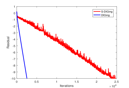
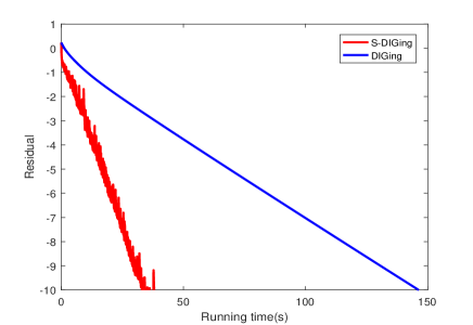
Refer to caption
(a) Evolution of residuals with number of iterations
Refer to caption
(b) Evolution of residuals with running time of algorithms
Figure 1: Comparison across S-DIGing and DIGing.

From Fig. 1, we find that the S-DIGing algorithm needs more iterations than the DIGing algorithm to achieve a same residual. However, it is worth to note that the S-DIGing algorithm has an advantage in running time on account of the smaller computational cost required for a single iteration.

V-A2 Effects of Fixed Step-Size and Scales of Network

Firstly, we compare the performance of the S-DIGing algorithm in terms of step-size selection. We choose m=100𝑚100m=100, qi=60subscript𝑞𝑖60q_{i}=60 for i=1,2,,m𝑖12𝑚i=1,2,\dots,m, and n=4𝑛4n=4. For each agent i𝑖i, half on the feature vectors ci,h4subscript𝑐𝑖superscript4c_{i,h}\in{{\mathbb{R}}^{4}} with label li,h=+1subscript𝑙𝑖1l_{i,h}=+1 are drawn by i.i.d 𝒩([2,2,2,2]T,2I)𝒩superscript2222T2𝐼\mathsf{\mathcal{N}}({{\left[2,2,-2,-2\right]}^{\text{T}}},2I) while the others with label li,h=1subscript𝑙𝑖1l_{i,h}=-1 are set to be i.i.d 𝒩([2,2,2,2]T,2I)𝒩superscript2222T2𝐼\mathsf{\mathcal{N}}({{\left[-2,-2,2,2\right]}^{\text{T}}},2I). Letting the step-size, α𝛼\alpha, equal to 0.002, 0.006, 0.010, 0.014, 0.018 and 0.022, respectively, Fig. 3 shows the evolutions of residuals respect to diverse step-sizes. The simulation is performed on the network shown in Fig. 4. From Fig. 3, we can find that the increasing of step-size plays a positive role in the execution of the S-DIGing algorithm within a certain range. If the step-size out of the range, the convergence of the S-DIGing algorithm will be deteriorated. Secondly, we choose m=50,75,100𝑚5075100m=50,75,100 and select α=0.001𝛼0.001\alpha=0.001 and qi=6000/msubscript𝑞𝑖6000𝑚q_{i}=6000/m to observe the performance of the algorithm under different scales of networks. Fig. 5 displays the evolutions of residuals respect to different scales of network.
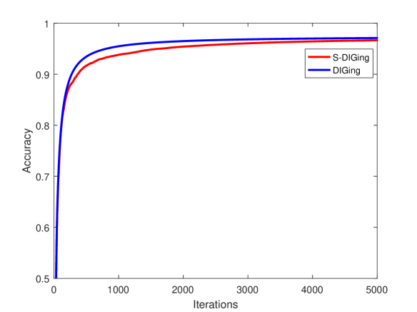
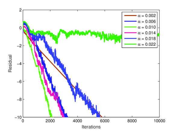
Refer to caption
Figure 2: Testing accuracy.
Refer to caption
Figure 3: Comparison across different step-sizes.
Refer to caption
Figure 4: Network topology.
Refer to caption
Figure 5: Comparison across different scales of network.

V-A3 Image Recognition

In this case, we solve the logistic regression problem in (49) for the MNIST database of handwritten digits provided in [38]. We randomly choose a subset of 580005800058000 handwritten digits from the MNIST database, where N=50000𝑁50000N=50000 samples from training set are used to train the discriminator x𝑥x and 8000 samples from testing set are used for testing. A part of training samples are shown in Fig. 6. The network used to solve this problem consists of m=10𝑚10m=10 agents and the probability of connection between each pair of agents is 40%percent4040\%. Each image, ci,h784subscript𝑐𝑖superscript784c_{i,h}\in{{\mathbb{R}}^{784}}, is a vector and the total images are divided among m𝑚m agents such that each agent has qisubscript𝑞𝑖q_{i} = 5000, i=1,2,,m𝑖12𝑚i=1,2,\dots,m, images. Due to privacy and communication restrictions, agents do not share their local training data with others. After the algorithm performs 1×1051superscript1051\times{{10}^{5}} iterations, the accuracy for each digit is shown in Table I.
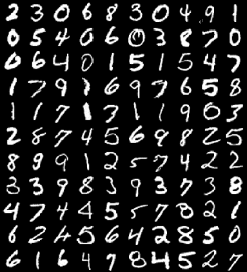
Refer to caption
Figure 6: Samples from the data set.
TABLE I: Testing accuracy for classification.
Digit 0 1 2 3 4
Accuracy 98.24% 98.99% 96.91% 94.28% 97.16%
Digit 5 6 7 8 9
Accuracy 95.47% 97.18% 97.38% 92.87% 93.14%

V-B Energy-Based Source Localization

Consider a sensor network composed of m𝑚m agents distributed at known spatial locations, denoted ri2subscript𝑟𝑖superscript2{{r}_{i}}\in{{\mathbb{R}}^{2}}, i=1,,m𝑖1𝑚i=1,\ldots,m. A stationary acoustic source is located at an unknown location x~2superscript~𝑥superscript2{{\tilde{x}}^{*}}\in{{\mathbb{R}}^{2}}. Let a>0𝑎0a>0 be a constant and υi,hsubscript𝜐𝑖{{\upsilon}_{i,h}} be i.i.d. samples of a zero-mean Gaussian noise process with variance σ2superscript𝜎2{{\sigma}^{2}} We use an isotropic energy propagation model for the hh-th received signal strength measurement at agent i𝑖i: ci,h=ax~riθ+vi,hsubscript𝑐𝑖𝑎superscriptnorm~𝑥subscript𝑟𝑖𝜃subscript𝑣𝑖{{c}_{i,h}}=\frac{a}{{{\left\|{\tilde{x}}-{{r}_{i}}\right\|}^{\theta}}}+{{v}_{i,h}} where x~ri>1norm~𝑥subscript𝑟𝑖1\left\|{\tilde{x}}-{{r}_{i}}\right\|>1 and θ1𝜃1\theta\geq 1 is an attenuation characteristic. The maximum-likelihood estimator for the source’s location is found by solving the problem

x~=argminx~2i=1m1qih=1qi(ci,hax~riθ)2superscript~𝑥~𝑥superscript2superscriptsubscript𝑖1𝑚1subscript𝑞𝑖superscriptsubscript1subscript𝑞𝑖superscriptsubscript𝑐𝑖𝑎superscriptnorm~𝑥subscript𝑟𝑖𝜃2\displaystyle{{\tilde{x}}^{*}}=\arg\underset{\tilde{x}\in{{\mathbb{R}}^{2}}}{\mathop{\min}}\,\sum\limits_{i=1}^{m}{\frac{1}{{{q}_{i}}}\sum\limits_{h=1}^{{{q}_{i}}}{{{\left({{c}_{i,h}}-\frac{a}{{{\left\|\tilde{x}-{{r}_{i}}\right\|}^{\theta}}}\right)}^{2}}}} (52)

The method that we use to solve this problem is proposed in [39]. According to the analysis given in [39], it can be found that the instantaneous function

fih=(ci,hax~riθ)2superscriptsubscript𝑓𝑖superscriptsubscript𝑐𝑖𝑎superscriptnorm~𝑥subscript𝑟𝑖𝜃2\displaystyle f_{i}^{h}={{\left({{c}_{i,h}}-\frac{a}{{{\left\|\tilde{x}-{{r}_{i}}\right\|}^{\theta}}}\right)}^{2}}

obtains its minimum on the circle

Ci,h={x~2:x~ri=a/ci,h}subscript𝐶𝑖conditional-set~𝑥superscript2norm~𝑥subscript𝑟𝑖𝑎subscript𝑐𝑖\displaystyle{{C}_{i,h}}=\left\{\tilde{x}\in{{\mathbb{R}}^{2}}:\left\|\tilde{x}-{{r}_{i}}\right\|=\sqrt{a/{{c}_{i,h}}}\right\}

Let Di,hsubscript𝐷𝑖D_{i,h} be the disk defined by

Di,h={x~2:x~ria/ci,h}subscript𝐷𝑖conditional-set~𝑥superscript2norm~𝑥subscript𝑟𝑖𝑎subscript𝑐𝑖\displaystyle{{D}_{i,h}}=\left\{\tilde{x}\in{{\mathbb{R}}^{2}}:\left\|\tilde{x}-{{r}_{i}}\right\|\leq\sqrt{a/{{c}_{i,h}}}\right\}

Then, the estimator is any point that minimizes the sum of squared distances to the sets Di,hsubscript𝐷𝑖{{D}_{i,h}}, i=1,,m𝑖1𝑚i=1,\ldots,m, h=1,,qi1subscript𝑞𝑖h=1,\ldots,{{q}_{i}}. We rewrite the problem (52) as follows:

x~=argminx~ni=1m1qih=1qix~𝒫Di,h(x~)2superscript~𝑥~𝑥superscript𝑛superscriptsubscript𝑖1𝑚1subscript𝑞𝑖superscriptsubscript1subscript𝑞𝑖superscriptnorm~𝑥subscript𝒫subscript𝐷𝑖~𝑥2\displaystyle{{{\tilde{x}}}^{*}}=\arg\underset{\tilde{x}\in{{\mathbb{R}}^{n}}}{\mathop{\min}}\,\sum\limits_{i=1}^{m}{\frac{1}{{{q}_{i}}}\sum\limits_{h=1}^{{{q}_{i}}}{{{\left\|\tilde{x}-{{\mathsf{\mathcal{P}}}_{{{D}_{i,h}}}}\left({\tilde{x}}\right)\right\|}^{2}}}} (53)

where 𝒫Di,h(x~)subscript𝒫subscript𝐷𝑖~𝑥{{\mathsf{\mathcal{P}}}_{{{D}_{i,h}}}}\left({\tilde{x}}\right) is the orthogonal projection of x~~𝑥{\tilde{x}} onto Di,hsubscript𝐷𝑖{{D}_{i,h}}.

Refer to caption
Figure 7: A part of paths displayed on top of contours of log-likelihood function.

We have simulated this scenario with 505050 sensors uniformly distributed in a 100×100100100100\times 100 square, and the source location chosen randomly. The source emits a signal with strength a=100𝑎100a=100 and each sensor makes 100100100 measurements. Fig. 7 depicts 101010 paths taken by the S-DIGing algorithm plotted on top of contours of the log likelihood.

V-C Distributed K-Means Clustering

A popular clustering method that minimizes the clustering error is the K-means algorithm [40]. Suppose that there is a data set P=i=1mh=1qipi,h𝑃superscriptsubscript𝑖1𝑚superscriptsubscript1subscript𝑞𝑖subscript𝑝𝑖P=\sum\nolimits_{i=1}^{m}{\sum\nolimits_{h=1}^{{{q}_{i}}}{{{p}_{i,h}}}}, where pi,hnsubscript𝑝𝑖superscript𝑛{{p}_{i,h}}\in{{\mathbb{R}}^{n}}. The K𝐾K-clustering aims at partitioning this data set into K𝐾K disjoint clusters C1,,CKsubscript𝐶1subscript𝐶𝐾{{C}_{1}},\ldots,{{C}_{K}}, such that a clustering criterion is optimized. The most widely used clustering criterion is the sum of the squared Euclidean distances between each data point pi,hsubscript𝑝𝑖p_{i,h} and the cluster center mlsubscript𝑚𝑙m_{l} of the subset which contains pi,hsubscript𝑝𝑖p_{i,h}. This criterion is called clustering error and depends on the cluster centers m1,,mKsubscript𝑚1subscript𝑚𝐾{{m}_{1}},\ldots,{{m}_{K}}:

minx~Knf(x~)=i=1mh=1qil=1Kai,hlpi,hml2~𝑥superscript𝐾𝑛𝑓~𝑥superscriptsubscript𝑖1𝑚superscriptsubscript1subscript𝑞𝑖superscriptsubscript𝑙1𝐾superscriptsubscript𝑎𝑖𝑙superscriptnormsubscript𝑝𝑖subscript𝑚𝑙2\displaystyle\underset{\tilde{x}\in{{\mathbb{R}}^{Kn}}}{\mathop{\min}}\,f\left({\tilde{x}}\right)=\sum\limits_{i=1}^{m}{\sum\limits_{h=1}^{{{q}_{i}}}{\sum\limits_{l=1}^{K}{a_{i,h}^{l}{{\left\|{{p}_{i,h}}-{{m}_{l}}\right\|}^{2}}}}} (54)

where x~=[m1T,.,mKT]T\tilde{x}={{[m_{1}^{\text{T}},.\ldots,m_{K}^{\text{T}}]}^{\text{T}}}, ai,hl=1superscriptsubscript𝑎𝑖𝑙1a_{i,h}^{l}=1 if pi,hClsubscript𝑝𝑖subscript𝐶𝑙{{p}_{i,h}}\in{{C}_{l}} and ai,hl=0superscriptsubscript𝑎𝑖𝑙0a_{i,h}^{l}=0 otherwise. Then, we solve the clustering problem for the Iris data set provided in UCI Machine Learning Repository [37]. The data set contains 3 classes of 50 samples, where each class refers to a type of iris plant. Each sample has 4 attributes included sepal length, sepal width, petal length and petal width. We set m=5𝑚5m=5, qi=30subscript𝑞𝑖30{{q}_{i}}=30, i=1,,m𝑖1𝑚i=1,\ldots,m, and the probability of connection between each pair of agents is 40%percent4040\%. Fig. 8 presents that although the S-DIGing algorithm needs more iterations than the DIGing algorithm to achieve a same residual. The S-DIGing algorithm has an advantage in running time due to the smaller computational cost required for a single iteration.
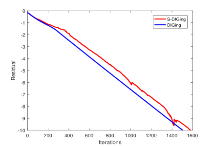
Refer to caption
(a) Evolution of residuals with number of iterations
Refer to caption
(b) Evolution of residuals with running time of algorithms
Figure 8: Comparison across S-DIGing and DIGing.

VI Conclusion

In this paper, a distributed stochastic gradient tracking algorithm which combines the gradient tracking algorithm with stochastic averaging gradient was proposed to solve the distributed optimization problem where each local objective function is constructed as an average of instantaneous functions. Employing the unbiased stochastic gradient technology, the cost of calculating the gradient of local objective function at each agent is greatly reduced. The theoretical analysis showed that the S-DIGing algorithm can linearly converge to the global optimal solution with explicit convergence rate when step-size is positive and less than an upper bound. We presented three numerical simulations to illustrate the effectiveness of the S-DIGing algorithm. Future work will focus on further improving the convergence rate and studying distributed optimization algorithm over time-varying and directed networks. For good measure, different from the synchronous update and communication required by the existing algorithm, asynchronous distributed optimization algorithm is also a promising research.

References

  • [1] S. Sardellitti, S. Barbarossa, and G. Scutari, “Distributed mobile cloud computing: Joint optimization of radio and computational resources,” 2014 IEEE Globecom Workshops, pp. 1505–1510, 2014.
  • [2] Q. Jia, L. Guo, Y. Fang, and G. Wang, “Efficient privacy-preserving machine learning in hierarchical distributed system,” IEEE Transactions on Network Science and Engineering, doi: 10.1109/TNSE.2018.2859420.
  • [3] D. Ardagna, C. Francalanci, and M. Trubian, “Joint optimization of hardware and network costs for distributed computer systems,” IEEE Transactions on Systems, Man, and Cybernetics - Part A: Systems and Humans, vol. 38, no. 2, pp. 470–484, 2008.
  • [4] H. Wang, X. Liao, T. Huang, and C. Li, “Cooperative distributed optimization in multiagent networks with delays,” IEEE Transactions on Systems, Man, and Cybernetics: Systems, vol. 45, no. 2, pp. 363–369, 2015.
  • [5] Z. Fan, “A distributed demand response algorithm and its application to PHEV charging in smart grids,” IEEE Transactions on Smart Grid, vol. 3, no. 3, pp. 1280–1290, 2012.
  • [6] K. Tsianos, S. Lawlor, and M. Rabbat, “Consensus-based distributed optimization: Practical issues and applications in large-scale machine learning,” 2012 50th Annual Allerton Conference on Communication, Control, and Computing, Allerton 2012, pp. 1543–1550, 2012.
  • [7] S. Yang, Q. Liu, and J. Wang, “A collaborative neurodynamic approach to multiple-objective distributed optimization,” IEEE Transactions on Neural Networks and Learning Systems, vol. 29, no. 4, pp. 981–992, 2018.
  • [8] D. Yuan, D. Ho, and S. Xu, “Zeroth-order method for distributed optimization with approximate projections,” IEEE Transactions on Neural Networks and Learning Systems, vol. 27, no. 2, pp. 284–294, 2016.
  • [9] E. Camponogara and L. Barcelos de Oliveira, “Distributed optimization for model predictive control of linear-dynamic networks,” IEEE Transactions on Systems, Man, and Cybernetics - Part A: Systems and Humans, vol. 39, no. 6, pp. 1331–1338, 2009.
  • [10] S. Yang, Q. Liu, and J. Wang, “Distributed optimization based on a multiagent system in the presence of communication delays,” IEEE Transactions on Systems, Man, and Cybernetics: Systems, vol. 47, no. 5, pp. 717–728, 2017.
  • [11] F. Guo, G. Li, C. Wen, L. Wang, and Z. Meng, “An accelerated distributed gradient-based algorithm for constrained optimization with application to economic dispatch in a large-scale power system,” IEEE Transactions on Systems, Man, and Cybernetics: Systems, pp. 1–13, 2019.
  • [12] Y. Nesterov, Introductory Lectures on Convex Optimization: A basic course. Springer Science & Business Media, 2004.
  • [13] S. Liu, Z. Qiu, and L. Xie, “Convergence rate analysis of distributed optimization with projected subgradient algorithm,” Automatica, vol. 83, pp. 162–169, 2017.
  • [14] A. Nedić, A. Olshevsky, Shi, and Wei, “Achieving geometric convergence for distributed optimization over time-varying graphs,” SIAM Journal on Optimization, vol. 27, no. 4, pp. 2597–2633, 2017.
  • [15] M. Maros and J. Jaldén, “Panda: A dual linearly converging method for distributed optimization over time-varying undirected graphs,” in 2018 IEEE Conference on Decision and Control (CDC), pp. 6520–6525, 2018.
  • [16] A. Nedić, A. Olshevsky, A. Ozdaglar, and J. N. Tsitsiklis, “Distributed subgradient methods and quantization effects,” Proceedings of the IEEE Conference on Decision and Control, pp. 4177–4184, 2008.
  • [17] A. Nedić and A. Ozdaglar, “Distributed subgradient methods for multi-agent optimization,” IEEE Transactions on Automatic Control, vol. 54, no. 1, pp. 48–61, 2009.
  • [18] I. Lobel and A. Ozdaglar, “Distributed subgradient methods for convex optimization over random networks,” IEEE Transactions on Automatic Control, vol. 56, no. 6, pp. 1291–1306, 2011.
  • [19] A. Mokhtari, Q. Ling, and A. Ribeiro, “Network Newton distributed optimization methods,” IEEE Transactions on Signal Processing, vol. 65, no. 1, pp. 146–161, 2017.
  • [20] E. Wei, A. Ozdaglar, and A. Jadbabaie, “A distributed newton method for network utility maximization - Part II: Convergence,” IEEE Transactions on Automatic Control, vol. 58, no. 9, pp. 2176–2188, 2013.
  • [21] S. Bolognani and S. Zampieri, “Distributed Quasi-Newton method and its application to the optimal reactive power flow problem,” IFAC Proceedings Volumes, vol. 43, no. 19, pp. 305–310, 2010.
  • [22] A. Lewis and M. Overton, “Nonsmooth optimization via quasi-Newton methods,” Mathematical Programming, vol. 141, no. 1-2, pp. 135–163, 2013.
  • [23] W. Lin, Y. Wang, C. Li, and J. Xiao, “Global optimization: A distributed compensation algorithm and its convergence analysis,” IEEE Transactions on Systems, Man, and Cybernetics: Systems, pp. 1–15, 2019.
  • [24] S. Boyd, N. Parikh, E. Chu, B. Peleato, and J. Eckstein, “Distributed optimization and statistical learning via the alternating direction method of multipliers,” Foundations and Trends in Machine Learning, vol. 3, no. 1, pp. 1–122, 2010.
  • [25] F. Iutzeler, P. Bianchi, P. Ciblat, and W. Hachem, “Explicit convergence rate of a distributed alternating direction method of multipliers,” IEEE Transactions on Automatic Control, vol. 61, no. 4, pp. 892–904, 2016.
  • [26] T. Chang, “A proximal dual consensus ADMM method for multi-agent constrained optimization,” IEEE Transactions on Signal Processing, vol. 64, no. 14, pp. 3719–3734, 2016.
  • [27] W. Shi, Q. Ling, G. Wu, and W. Yin, “Extra: An exact first-order a lgorithm for decentralized consensus optimization,” SIAM Journal on Optimization, vol. 25, pp. 944–966, apr 2015.
  • [28] M. Schmidt, N. Roux, and F. Bach, “Minimizing finite sums with the stochastic average gradient,” Mathematical Programming, vol. 162, no. 1-2, pp. 83–112, 2017.
  • [29] A. Mokhtari and A. Ribeiro, “Decentralized double stochastic averaging gradient,” Conference Record - Asilomar Conference on Signals, Systems and Computers, vol. 2016-Febru, pp. 406–410, 2016.
  • [30] A. Defazio, F. Bach, and S. Lacoste-Julien, “SAGA: A fast incremental gradient method with support for non-strongly convex composite objectives,” Advances in Neural Information Processing Systems, vol. 2, no. January, pp. 1646–1654, 2014.
  • [31] Z. Wang and H. Li, “Edge-based stochastic gradient algorithm for distributed optimization,” IEEE Transactions on Network Science and Engineering, doi: 10.1109/TNSE.2019.2933177.
  • [32] R. Xin and U. Khan, “A linear algorithm for optimization over directed graphs with geometric convergence,” IEEE Control Systems Letters, vol. 2, no. 3, pp. 313–318, 2018.
  • [33] R. Xin, A. Sahu, U. Khan, and S. Kar, “Distributed stochastic optimization with gradient tracking over strongly-connected networks,” arxiv: 1903.07266.
  • [34] H. Wai, N. Freris, A. Nedić, and A. Scaglione, “SUCAG: Stochastic unbiased curvature-aided gradient method for distributed optimization,” Proceedings of the IEEE Conference on Decision and Control, vol. 2018, pp. 1751–1756, 2019.
  • [35] J. Chen, K. Yao, and R. Hudson, “Source localization and beamforming,” IEEE Signal Processing Magazine, vol. 19, no. 2, 2002.
  • [36] M. Grant and S. Boyd, “CVX: Matlab software for disciplined convex programming, ver 2.1,” Available at http://cvxr.com/cvx/, 2017.
  • [37] D. Dua and C. Graff, “UCI machine learning repository,” University of California, Irvine, School of Information and Computer Sciences, 2017.
  • [38] Y. LeCun, C. Cortes, and C. Burges, “MNIST handwritten digit database,” AT&T Labs [Online]. Available: http://yann. lecun. com/exdb/mnist, 2010.
  • [39] D. Blatt and A. Hero, “Energy-based sensor network source localization via projection onto convex sets,” IEEE Transactions on Signal Processing, vol. 54, no. 9, pp. 3614–3619, 2006.
  • [40] A. Likas, N. Vlassis, and J. Verbeek, “The global k-means clustering algorithm,” Pattern recognition, vol. 36, no. 2, pp. 451–461, 2003.