Application of a new information priority accumulated grey model with time power to predict short-term wind turbine capacity

Abstract

Wind energy makes a significant contribution to global power generation. Predicting wind turbine capacity is becoming increasingly crucial for cleaner production. For this purpose, a new information priority accumulated grey model with time power is proposed to predict short-term wind turbine capacity. Firstly, the computational formulas for the time response sequence and the prediction values are deduced by grey modeling technique and the definite integral trapezoidal approximation formula. Secondly, an intelligent algorithm based on particle swarm optimization is applied to determine the optimal nonlinear parameters of the novel model. Thirdly, three real numerical examples are given to examine the accuracy of the new model by comparing with six existing prediction models. Finally, based on the wind turbine capacity from 2007 to 2017, the proposed model is established to predict the total wind turbine capacity in Europe, North America, Asia, and the world. The numerical results reveal that the novel model is superior to other forecasting models. It has a great advantage for small samples with new characteristic behaviors. Besides, reasonable suggestions are put forward from the standpoint of the practitioners and governments, which has high potential to advance the sustainable improvement of clean energy production in the future.

Nomenclature
GM(1,1)	the basic grey system model
NGM(1,$N)$	non-linear grey multivariable models
NGM(1,1,$k$)	non-homogeneous exponential grey model
GMCN(1,$N$)	new information priority accumulated grey multivariable convolution model
NGM(1,1,$k,c$)	extended non-homogeneous exponential grey model
GAGM(1,1)	non-equidistance generalized accumulated grey forecasting model
DGM(1,1)	discrete grey model
NIPDGM(1,1)	new information priority accumulated discrete grey model
GMC(1,$N$)	convolution integral grey prediction model
GRM(1,1)	non-equidistant grey model based on reciprocal accumulated generating
FAGM(1,1)	fractional-order grey model
FDGM	fractional multivariate discrete grey model
NIPGM$(1,1,{t}^{\alpha})$	new information priority accumulated grey model with time power
1-AGO	first-order accumulative generation operation
1-IAGO	first-order inverse accumulative generation operation
1-NIPAGO	first-order new information priority accumulated generation operation
1-NIPIAGO	first-order new information priority inverse accumulated generation operation
${{S}^{0}}$	the non-negative original sequence
${{S}^{1}}$	first-order new information priority accumulated generation operation sequence
${{S}^{-1}}$	first-order new information priority inverse accumulated generation operation
$H^{1}$	the mean generation sequence with consecutive neighbors
$\lambda$	the accumulation generation parameter
$a,b,c$	the parameters of the grey system
$s_{k}^{0}$	the observational data for the system input at time $k$
$s_{k}^{1}$	the 1-NIPAGO data at time $k$
$s_{k}^{-1}$	the 1-NIPIAGO data at time $k$
$\hat{s}_{k}^{0}$	the prediction value at time $k$
$\hat{s}_{k}^{1}$	the time response value at time $k$
$h_{k}^{1}$	the background value at time $k$
${\rm APE}$	the absolute percentage error
${\rm RMSEPR}$	the root mean square error of prior-sample
${\rm RMSE}$	the root mean square error
${\rm RMSEPO}$	the root mean square error of post-sample
${\rm PR}(n)$	polynomial regression model
PSO	particle swarm optimization
${\rm ARIMA}(p,d,q)$	autoregressive integrated moving average model
CWEC	Global Wind Energy Council

1 Introduction

With the global energy crisis and environmental pollution, clean and renewable energy has received extensive attention in recent years[Pali & Vadhera, 2018, Lu et al., 2019]. Wind energy is one of the most rapidly growing clean energies, which produces a great deal of electrical energy by wind turbines [Shoaib et al., 2019]. Wind power generation accounts for an increasing proportion in the global power production structure[Moraes et al., 2018]. As reported by BP in Statistical Review of World Energy 2018, global wind turbine capacity growth averaged 20.2% per year in the past decade. And the wind turbine capacity of Asia, Europe, and North America accounted for 95.6% of the world, while other regions accounted for only 4.4% in 2017. Recently, the Global Wind Energy Council(CWEC) said that the wind power capacity of the world is expected to increase by 50% and exceed more than 300 million kilowatts by 2023. Wind energy has significant advantages and good development prospects in the development of cleaner production[Kiaee et al., 2018]. The reason is that it can reduce carbon dioxide emissions and fossil fuels burning[Wang & Li, 2019, Ma et al., 2019b]. Therefore, it is an inevitable choice for the global long-term energy strategy to develop wind energy, which can ensure sufficient energy supply[Zeng & Li, 2016]. Hence, accurately predicting the wind turbine capacity in Asia, Europe, North America, and the world is very important for decision-makers.

In the previous studies, many scholars have proposed many models to forecast the wind turbine capacity, including logistic model[Shafiee, 2015], autoregressive sliding average model[Jiang et al., 2012], time series analysis[Safari et al., 2018], support vector regression[Zendehboudi et al., 2018], neural network prediction model[Chang et al., 2017], combined forecasting model[Liu et al., 2018], grey machine learning[Ma, 2019, Wang et al., 2018b], and grey model[Wu et al., 2018c, Zeng et al., 2019]. Among the many forecasting methods, the regression analysis method uses the indicators related to the wind turbine capacity to build the model, which requires lots of samples. The calculation principle of time series model is simple but can not reflect its intrinsic influencing factors. The artificial neural network forecasting model has excellent predictive ability for nonlinear data. But it is difficult to search the optimal solution so that it cannot meet the accuracy requirements. However, the grey model differs from other forecasting models that it requires a small sample with just 4 data or more. Collecting sufficient samples is challenging in practical applications. Thus, more and more scholars have extensively concerned the grey system model.

Grey system theory along with grey models are initially put forward by Deng [1982] to solve uncertain problems. Because of the practicability of the grey model, the grey system has become a research direction with distinctive characteristics. The classical GM$(1,1)$ model has been generalized to other effective grey forecasting models, including NGM$(1,1,k)$[Cui et al., 2009], DGM$(1,1)$[Hu et al., 2009], NGM(1,$N)$ [Wang & Ye, 2017], and CFGM[Ma et al., 2019c]. These grey models have been successfully applied in the environment[Wu et al., 2018a], economy[Yin et al., 2018], energy[Wu et al., 2019] and other related fields[Wang et al., 2018a, Duan et al., 2019]. From the idea of GM $(1,1)$ modeling, it is the least-squares modeling method that follows the law of accumulated grey-index. And the traditional GM$(1,1)$ model has great forecasting effect on the data with homogeneous exponential law, and improved models have this characteristic. There are a large number of systematic development laws that do not conform to the exponential law in real life. For the data with partial exponential features and time power terms, Qian et al. [2012] constructed a novel GM $(1,1,{t}^{\alpha})$ model. However, these grey models are built by using the first-order accumulative generation operation (1-AGO)[Deng, 1982]. And the restored values of these models are deduced by using the first-order inverse accumulative generation operation (1-IAGO). Therefore, sequence accumulation generation is one of the critical steps of grey information mining and modeling.

In many references, the research on grey accumulation generation is mainly divided into two categories.

1) The idea of accumulation generation is combined with other forecasting models. Sheng et al. [2008] put forward a GSVMG model, and it was used to forecast patent application filings, which obtained higher prediction accuracy. Liu et al. [2011] developed a GMRBF $(2,1)$ model by combining the RBF neural network with grey accumulation generation, which was successfully applied to forecast ship carrying capacity. Recently, it is noteworthy that Zhou et al. [2017] defined the new accumulated generation operator with a parameter. And then a NIPDGM(1,1) was constructed, which obtained an excellent prediction effect in energy prediction of Jiangsu province. Later, Wu & Zhang [2018] proposed the GMCN(1, $N)$ model by combining the new information priority principle with GM(1, $N$) model.

2) The expansion of the grey accumulation generation technology. Liu et al. [2010] established a new grey GAGM(1, $1)$ model by generalized accumulative generation operation. This model was suitable for the unequal spacing sequences with the jumping trend and multistage. Based on the parallel number cumulative generation operation, the new grey GRM$(1,1)$ model was proposed by Xiao et al. [2012], which had practicality and reliability. To reduce the perturbation of the grey model solution, Wu et al. [2013] introduced a fractional-order accumulation method and constructed a new FAGM(1,1) model. Later, a new seasonal discrete grey prediction model with periodic effects was proposed by Xia & Wong [2014], which was successfully applied to forecast fashion consumer goods. Recently, Ma et al. [2019e] constructed the FDGM model and optimized it with the Gray Wolf algorithm.

Through the review and analysis of the above literature, it can be noticed that many models do not consider the new information priority principle. This may be the reason for the poor prediction accuracy. In order to solve this challenge for grey GM$(1,1,{t}^{\alpha})$ model, this study constructs a novel new information priority accumulated grey model with time power. Furthermore, the computational formulas for the sequence of time response and the values of prediction are deduced. Another problem of the current grey model with new information priority accumulation[Wu & Zhang, 2018] is that no detailed optimization algorithm has been used to seek the optimum solution of parameters. Therefore, we establish an optimization model to search the parameters and use the PSO algorithm to determine the optimized values of the novel model. Then, the novel model is applied to predict wind turbine capacity in Europe, North America, Asia, and the world. The numerical calculation results are compared with several existing models. Finally, according to the prediction results of wind turbine capacity in these regions from 2018 to 2020, reasonable suggestions on clean energy production are provided.

The remainder of this research is structured as below: Section 2 systematically discusses the novel grey model. Section 3 gives how to optimize the nonlinear parameters of the novel model by an intelligent algorithm. Section 4 validates the accuracy of the novel model through three real cases. Section 5 predicts wind turbine capacity by using seven forecasting models, and Section 6 gives the conclusions of the study.

2 The new information priority accumulated grey model with time power

2.1 Definition of new information priority accumulation

Definition 1

(see Zhou et al. [2017]) Set the non-negative historical data sequence as ${{S}^{0}}$ $=\left\{s_{k}^{0}|k\in 1,2,\cdots,m\right\}$, the first-order new information priority accumulated generation operation sequence (1-NIPAGO) of ${{S}^{0}}$ is ${{S}^{1}}=\left\{s_{k}^{1}|k\in 1,2,\cdots,m\right\}$. There is

$$s_{k}^{1}=\sum_{v=1}^{k}\lambda^{k-v}s_{v}^{0},\quad\lambda\in(0,1),k\in 1,2,3,\cdots,m,$$ (1)

and $\lambda$ presents the accumulation generation parameter, which is used to adjust the weight of the sequence. Eq.(1) is named new information priority accumulation.

In previous studies, Wu & Zhang [2018] proved that the weight of “new” 1-NIPAGO series $s_{k}^{1}$ is larger than the “old” ones. Being similar to the traditional grey model accumulation generation, ${{S}^{0}}$ can be accumulated and generated multiple times according to the accumulation mentioned above, and the multiple new information of ${{S}^{0}}$ can obtain the priority accumulation generation sequence ${{S}^{n}}$.

Definition 2

(see Zhou et al. [2017]) Assuming the first-order new information priority inverse accumulated generation operation sequence (1-NIPIAGO) of ${{S}^{0}}$ is ${{S}^{-1}}=\left\{s_{k}^{-1}|k\in 1,2,\cdots,m\right\}$, where

$$\left\{\begin{array}[]{l}{s_{k}^{-1}=s_{k}^{0}-\lambda s_{k-1}^{0}}\\ {s_{1}^{-1}=s_{1}^{0}}\end{array}\right.,\quad\lambda\in(0,1),k\in 2,3,4,\cdots,m.$$ (2)

It is worth noting that new information priority accumulated and new information priority inverse accumulated have the following relationship, these is

$$s_{k}^{1}-\lambda s_{k-1}^{1} =\sum_{v=1}^{k}\lambda^{k-v}s_{v}^{0}-\lambda\sum_{v=1}^{k-1}\lambda^{k-v-1}s_{v}^{0} =s_{k}^{0}.$$ (3)

The Eq.(3) is particularly important when establishing grey forecasting models and calculating prediction values for the original sequence, as shown below.

2.2 The definite integral trapezoidal approximation formula

In this subsection, the problem of estimating the value of the integral $\int_{{{d}_{1}}}^{{{d}_{2}}}{f(u)du}$ is discussed. First, the interval $\left[{{d}_{1}},{{d}_{2}}\right]$ is divided into $k$ sub-intervals of width $\Delta d=\frac{{{d}_{2}}-{{d}_{1}}}{k}$, and each sub-interval can be expressed as: $\left[{{\gamma}_{0}},{{\gamma}_{1}}\right],\cdots,\left[{{\gamma}_{k-1}},{{\gamma}_{k}}\right]$, where ${{\gamma}_{0}}={{d}_{1}}$ , ${{\gamma}_{k}}={{d}_{2}}$ .

Further, let the function value of each point ${{\gamma}_{0}},{{\gamma}_{1}},{{\gamma}_{2}},\cdots,{{\gamma}_{k}}$ of $f(u)$ correspond to $f(\gamma_{0}),f(\gamma_{1}),f(\gamma_{2})$, $\cdots,$ $f(\gamma_{k})$, as shown in Fig. 1.

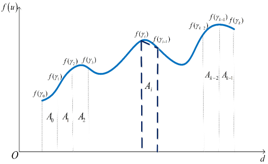
Figure 1: The diagram of trapezoidal formula to estimate curve integral.

Then the area of each narrow trapezoid is:

$$A_{i}=\frac{\Delta d}{2}\left(f\left(\gamma_{i}\right)+f\left(\gamma_{i+1}\right)\right).$$ (4)

Therefore, if there are $k$ sub-intervals, the integral can be approximated as

$$\int_{d_{1}}^{d_{2}}f(u)du\approx\frac{\Delta d}{2}\sum_{i=0}^{k-1}\left(f\left(\gamma_{i}\right)+f\left(\gamma_{i+1}\right)\right),$$ (5)

which is the definite integral trapezoidal approximate formula.

2.3 Modeling process of NIPGM$(1,1,{t}^{\alpha})$ model

The tradition grey model with time power was established by Qian et al. [2012]. In the following, the novel new information priority accumulated grey model with time power is defined as.

Definition 3

Set the non-negative original sequence as ${{S}^{0}}$, the 1-NIPAGO of ${{S}^{0}}$ is ${{S}^{1}}$, ${{s}_{k}^{1}}$ is shown in Eq.(1). The mean generation sequence with consecutive neighbors is $H^{1}=\left\{h_{k}^{1}|k\in 2,3,\cdots,m\right\}$, where $h_{k}^{1}=0.5s_{k}^{1}+0.5s_{k-1}^{1}$.

Definition 4

Set ${{S}^{0}}$, ${{S}^{1}}$ and ${{H}^{1}}$ be shown in Definition 3, there is

$$s_{k}^{0}+ah_{k}^{1}=bk^{\alpha}+c,$$ (6)

is named the mathematical form of NIPGM(1,1,${{t}^{\alpha}}$), then,

$$\frac{ds_{t}^{1}}{dt}+as_{t}^{1}=bt^{\alpha}+c,$$ (7)

which is named the whitening equation of NIPGM (1,1,${{t}^{\alpha}}$). $\alpha$ presents a non-negative constant, $a$ presents development coefficient, and the amount of grey action is $b{{t}^{\alpha}}+c$.

The Eq.(7) is integral on interval $\left[k-1,k\right]$, there is

$$s_{k}^{1}-s_{k-1}^{1}+0.5a\left(s_{k}^{1}+s_{k-1}^{1}\right)=b\frac{k^{1+\alpha}-(k-1)^{1+\alpha}}{1+\alpha}+c,$$ (8)

Because of $h_{k}^{1}=0.5s_{k}^{1}+0.5s_{k-1}^{1}$, Eq.(8) turns to be

$$s_{k}^{1}-s_{k-1}^{1}+ah_{k}^{1}=b\frac{k^{1+\alpha}-(k-1)^{1+\alpha}}{1+\alpha}+c,$$ (9)

Further, there is

$$-ah_{k}^{1}+b\frac{k^{1+\alpha}-(k-1)^{1+\alpha}}{1+\alpha}+c=s_{k}^{1}-s_{k-1}^{1},$$ (10)

Theorem 1

Suppose ${{S}^{0}}$, ${{S}^{1}}$ and ${{H}^{1}}$ are defined in Definition 3, $\hat{r}={{\left[a,b,c\right]}^{T}}$ is a parameter column, the least-squares parameter estimate of the novel model satisfies $\hat{r}={{({{F}^{T}}F)}^{-1}}{{F}^{T}}G$, where

$$F=\left(\begin{matrix}-h_{2}^{1}&\frac{{{2}^{1+\alpha}}-1}{1+\alpha}&1\\ -h_{3}^{1}&\frac{{{3}^{1+\alpha}}-{{2}^{1+\alpha}}}{1+\alpha}&1\\ \vdots&\vdots&\vdots\\ -h_{m}^{1}&\frac{{{m}^{1+\alpha}}-{{(m-1)}^{1+\alpha}}}{1+\alpha}&1\\ \end{matrix}\right),G=\left(\begin{matrix}s_{2}^{1}-s_{1}^{1}\\ s_{3}^{1}-s_{2}^{1}\\ \vdots\\ s_{m}^{1}-s_{m-1}^{1}\\ \end{matrix}\right).$$ (11)

Proof 1

Using the method of the mathematical induction, take $k=2,3,\cdots,m$ into Eq.(10), there is

$$\left\{\begin{array}[]{l}{a\left(-h_{2}^{1}\right)+b\frac{2^{1+\alpha}-1}{1+\alpha}+c=s_{2}^{1}-s_{1}^{1}}\\ {a\left(-h_{3}^{1}\right)+b\frac{3^{1+\alpha}-2^{1+\alpha}}{1+\alpha}+c=s_{3}^{1}-s_{2}^{1}}\\ ~{}~{}~{}~{}~{}~{}~{}~{}~{}~{}~{}~{}~{}~{}~{}~{}~{}~{}~{}~{}~{}~{}~{}~{}~{}~{}~{}~{}~{}\vdots\\ {a\left(-h_{m}^{1}\right)+b\frac{m^{1+\alpha}-(m-1)^{1+\alpha}}{1+\alpha}+c=s_{m}^{1}-s_{m-1}^{1}}\end{array}\right.$$ (12)

Convert the Eq.(12) into the matrix form, then

$$\left(\begin{matrix}-{h_{2}^{1}}&\frac{{{2}^{1+\alpha}}-1}{1+\alpha}&1\\ -{h_{3}^{1}}&\frac{{{3}^{1+\alpha}}-{{2}^{1+\alpha}}}{1+\alpha}&1\\ \vdots&\vdots&\vdots\\ -{h_{m}^{1}}&\frac{{{m}^{1+\alpha}}-{{(m-1)}^{1+\alpha}}}{1+\alpha}&1\\ \end{matrix}\right)\left(\begin{matrix}a\\ b\\ c\\ \end{matrix}\right)=\left(\begin{matrix}s_{2}^{1}-s_{1}^{1}\\ s_{3}^{1}-s_{2}^{1}\\ \vdots\\ s_{m}^{1}-s_{m-1}^{1}\\ \end{matrix}\right).$$ (13)

In summary

$$\hat{r}=\left(\begin{array}[]{l}{a}\\ {b}\\ {c}\end{array}\right)=\left(F^{T}F\right)^{-1}F^{T}G.$$ (14)

Theorem 2

Suppose $F$, $G$, $\hat{r}$ are described in Theorem 1, the sequence of time response $\hat{s}_{k}^{1}$ of the NIPGM(1,1,${{t}^{\alpha}}$) model is:

$$\hat{s}_{k}^{1}=\left(s_{1}^{0}-\frac{c}{a}\right)e^{-a(k-1)}+\frac{b}{2}e^{-a(k-1)}\sum_{\gamma=1}^{k-1}\left\{\gamma^{\alpha}e^{a(\gamma-1)}+(\gamma+1)^{\alpha}e^{a\gamma}\right\}+\frac{c}{a},\quad k=2,3,\cdots,m,$$ (15)

then the restored values of $\hat{s}_{k+1}^{0}$ can be deduced by using the 1-NIPIAGO,

$$\hat{s}_{k+1}^{0}= e^{-a(k-1)}\left(e^{-a}-\lambda\right)\left\{s_{1}^{0}+\frac{b}{2}\sum_{\gamma=1}^{k-1}\left\{\gamma^{\alpha}e^{a(\gamma-1)}+(\gamma+1)^{\alpha}e^{\alpha\gamma}\right\}\right\}$$ (16)

$$+\frac{b}{2}\left\{k^{\alpha}e^{-a}+(k+1)^{\alpha}\right\}+\frac{c}{a}\left(1-e^{-a}\right),\quad k=2,3,\cdots,m.$$

Proof 2

We all know the general solution of linear non-homogeneous differential equation Eq.(7) is composed of the solution of its corresponding homogeneous equation plus one of its special solution. For Eq.(7), its homogeneous form as:

$$\frac{ds_{t}^{1}}{dt}+as_{t}^{1}=0,$$ (17)

then we solve the general solution of Eq.(17) is $\ln s_{t}^{1}=-at+c$. Further, simplification gives $s_{t}^{1}=Qe^{-at}$. Taking $t=1$, there is $Q=e^{at}s_{1}^{1}$, $c$ and $Q$ is a constant.

Using the constant variation method, we obtain the solution of Eq.(7) as

$$s_{t}^{1}=Q(t)e^{-at},$$ (18)

Because of $Q(t)=s_{t}^{1}e^{at}$ and $s_{t}^{1}=s_{t}^{0}$, then $Q(1)=e^{a}s_{1}^{0}$. Bringing Eq.(18) into Eq.(7), we get

$$\frac{dQ(t)}{dt}=e^{at}\left(bt^{\alpha}+c\right),$$ (19)

Further, considering the integral of Eq.(19) on the interval $\left[1,t\right]$, we can obtain

$$\int_{1}^{t}dQ(u)=\int_{1}^{t}e^{au}\left(bu^{\alpha}+c\right)du,$$ (20)

From Eq.(20) know that

$$Q(t)-Q(1)=b\int_{1}^{t}u^{\alpha}e^{au}du+\frac{c}{a}\left(e^{at}-e^{a}\right),$$ (21)

Thus, $Q(t)$ can be represented as

$$\left\{\begin{array}[]{l}{Q(t)=Q(1)+b\int_{1}^{t}u^{\alpha}e^{au}du+\frac{c}{a}\left(e^{at}-e^{a}\right)}\\ {Q(t)=e^{at}s_{t}^{1}}\end{array}.\right.$$ (22)

According to Eq.(22) and the definite integral trapezoidal approximation formula Eq.(5), the continuous-time response function $s_{t}^{1}$ can be derived from the following formula,

$$s_{t}^{1} =\left(Q(1)+b\int_{1}^{t}u^{\alpha}e^{au}du+\frac{c}{a}\left(e^{at}-e^{a}\right)\right)e^{-at}$$ (23)

$$=\left(s_{1}^{0}-\frac{c}{a}\right)e^{-a(t-1)}+be^{-a(t-1)}\int_{1}^{t}u^{\alpha}e^{a(u-1)}du+\frac{c}{a}$$

$$=\left(s_{1}^{0}-\frac{c}{a}\right)e^{-a(t-1)}+\frac{c}{a}$$

$$+\frac{b}{2}e^{-a(t-1)}\sum_{\gamma=1}^{t-1}\left\{\gamma^{\alpha}e^{a(\gamma-1)}+(\gamma+1)^{\alpha}e^{a\gamma}\right\}.$$

Finally, the continuous-time response function is challenging to calculate in actual applications[Ma et al., 2019d], so we further discrete Eq.(23) to obtain the time response sequence $\hat{s}_{k}^{1}$ . And the prediction values of $\hat{s}_{k}^{0}$ can be solved by using Eq.(3).

2.4 Generality of the NIPGM(1, 1, ${{t}^{\alpha}}$) model

The novel grey model is a more extensive model, which combines new information priority accumulation with grey model with time power. Fig.2 displays that the relationship between the novel model and the classical GM(1, 1)model[Deng, 1982], non-homogeneous exponential NGM(1, 1, $k$) model [Cui et al., 2009], extended non-homogeneous exponential NGM(1, 1, $k$, $c$) model[Wang et al., 2014], and grey GM(1, 1, ${{t}^{\alpha}}$)model with time power[Qian et al., 2012].

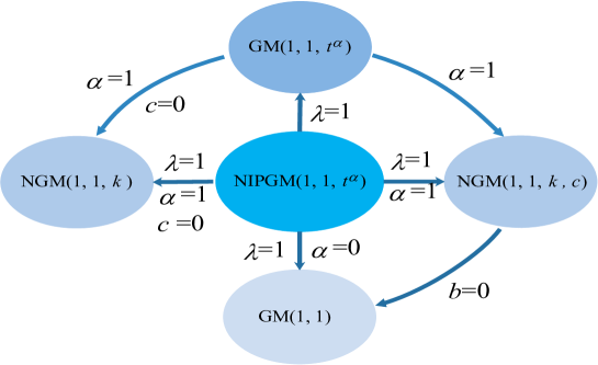
Figure 2: The relationship of the novel model to other prediction models.

i) If $\alpha\text{=}0$ and $\lambda\text{=}1$, the proposed model becomes $s_{k}^{0}+ah_{k}^{1}=bk^{0}+c=b_{0}$, which degenerates into the classical GM(1, 1) model, then

1) The sequence of time response $\hat{s}_{k}^{1}$ as

$$\hat{s}_{k}^{1}=\left({s}_{1}^{1}-\frac{b_{0}}{a}\right)e^{-a(k-1)}+\frac{b_{0}}{a},$$ (24)

2)The values of prediction $\hat{s}_{k+1}^{0}$ as

$$\hat{s}_{k+1}^{0}=\left(1-e^{a}\right)\left({s}_{1}^{0}-\frac{b_{0}}{a}\right)e^{-ak}.$$ (25)

ii) If $\alpha\text{=1}$ and $\lambda\text{=}1$, the new model becomes $s_{k}^{0}+ah_{k}^{1}=bk+c$, which reduces into the NGM(1, 1, $k$, $c$) model, then

$$\int_{1}^{t}ue^{a(u-1)}du=\frac{(at-1)e^{a(t-1)}+(1-a)}{a^{2}},$$

there are

1) The sequence of time response $\hat{s}_{k}^{1}$ as

$$\hat{s}_{k}^{1}=\left({s}_{1}^{1}-\frac{ab+ac-b}{a^{2}}\right)e^{-a(k-1)}+\frac{b}{a}(k-1)+\frac{ac-b}{a^{2}},$$ (26)

2)The values of prediction $\hat{s}_{k+1}^{0}$ as

$$\hat{s}_{k+1}^{0}=\left(1-e^{a}\right)\left({s}_{1}^{0}-\frac{ab+ac-b}{a^{2}}\right)e^{-ak}+\frac{b}{a}.$$ (27)

iii) If $\alpha\text{=1}$,$\lambda\text{=}1$ and $c=0$, the proposed model becomes $s_{k}^{0}+ah_{k}^{1}=bk$, which degenerates into the NGM(1, 1, $k$) model, there are

1) The sequence of time response $\hat{s}_{k}^{1}$ as

$$\hat{s}_{k}^{1}=\left({s}_{1}^{1}+\frac{b-ab}{a^{2}}\right)e^{-a(k-1)}+\frac{b}{a}(k-1)-\frac{b}{a^{2}},$$ (28)

2) The values of prediction $\hat{s}_{k+1}^{0}$ as

$$\hat{s}_{k+1}^{0}=\left(1-e^{a}\right)\left({s}_{1}^{0}+\frac{b-ab}{a^{2}}\right)e^{-ak}+\frac{b}{a}.$$ (29)

iv) If $\lambda\text{=}1$, the proposed model becomes $s_{k}^{0}+ah_{k}^{1}=bk^{2}+c$, which reduces into the GM(1, 1, ${{t}^{\alpha}}$) model with time power, then

1) The sequence of time response $\hat{s}_{k}^{1}$ as

$$\hat{s}_{k}^{1}=\left({s}_{1}^{0}-\frac{c}{a}\right)e^{-a(k-1)}+\frac{b}{2}e^{-a(k-1)}\sum_{\gamma=1}^{k-1}\left\{\gamma^{\alpha}e^{a(\gamma-1)}+(\gamma+1)^{\alpha}e^{a\gamma}\right\}+\frac{c}{a},\quad k\in 2,3,\cdots,m,$$ (30)

2) The values of prediction $\hat{s}_{k+1}^{0}$ as

$$\hat{s}_{k+1}^{0}= e^{-a(k-1)}\left(e^{-a}-1\right)\left\{s_{1}^{0}+\frac{b}{2}\sum_{\gamma=1}^{k-1}\left\{\gamma^{\alpha}e^{a(\gamma-1)}+(\gamma+1)^{\alpha}e^{\alpha\gamma}\right\}\right\}$$ (31)

$$+\frac{b}{2}\left\{k^{\alpha}e^{-a}+(k+1)^{\alpha}\right\}+\frac{c}{a}\left(1-e^{-a}\right),\quad k\in 2,3,\cdots,m.$$

It can be seen from Eq.(25), Eq.(27) and Eq.(29) that the classical GM(1, 1) model, NGM(1, 1, $k$, $c$) model, and NGM(1, 1, $k$) model are suitable for sequences with non-homogeneous exponential law ${s}_{t}^{0}\approx de^{at}+p$. However, both Eq.(16) and Eq.(31) are composed of power functions and exponential functions. The grey model with time power and the novel model can be applied to sequences with partial exponential features and time power terms ${s}_{t}^{0}\approx de^{at}+pt^{\alpha}+q$. The difference between the grey model with time power and the new model is the way of sequence accumulation generation. The GM(1, 1, ${{t}^{\alpha}}$) model does not successfully apply the new information priority principle. Therefore, the proposed model is suitable for situations where the data characteristics are complex, which has more excellent flexibility and practicality than the other four models.

3 Optimization of the parameters by particle swarm optimization

We can notice that the parameters $\lambda$ and $\alpha$ have been given before building the NIPGM (1,1,${{t}^{\alpha}}$) model. Choosing the optimal parameters $\lambda$ and $\alpha$ is very important, which can enhance the fitting and predicting capabilities of the proposed model. The details about how to optimize the parameters $\lambda$ and $\alpha$ by the particle swarm optimization algorithm were given in this section.

3.1 Model evaluation criteria

To examine the accuracy of each forecasting model, we select the absolute percentage error (APE), the root mean square error of priori-sample (RMSEPR)[Ma & Liu, 2017], the root mean square error of the post-sample (RMSEPO)[Wu et al., 2018b] and the root mean square error (RMSE)[Ma & Liu, 2017] as the assessment standard. These expressions are expressed as

$${\rm APE}(k)=\left|\frac{{s}_{k}^{0}-\hat{s}_{k}^{0}}{{s}_{k}^{0}}\right|\times 100\%,$$ (32)

$${\rm RMSEPR}=\sqrt{\frac{1}{l}\sum_{k=1}^{l}\left({\rm APE}(k)\right)^{2}}\times 100\%,$$ (33)

$${\rm RMSEPO}=\sqrt{\frac{1}{m-l}\sum_{k=l+1}^{m}\left({\rm APE}(k)\right)^{2}}\times 100\%,$$ (34)

$${\rm RMSE}=\sqrt{\frac{1}{m}\sum_{k=1}^{m}\left({\rm APE}(k)\right)^{2}}\times 100\%.$$ (35)

where, $l$ presents the amount of sample applied to establish forecasting model, $m$ presents the total amount of sample.

3.2 Nonlinear optimization model for the parameters $\lambda$ and $\alpha$

When using the NIPGM (1,1,${{t}^{\alpha}}$) model to forecast the original data, we first need to determine the parameters $\lambda$ and $\alpha$ of the model, then use Eq.(11) to obtain the parameters $(a,b,c)$, and use Eq.(16) to solve the prediction values $\hat{s}_{k}^{0}$. In this paper, the minimum RMSE corresponding $\lambda$ and $\alpha$ are used as the optimal model parameters, and its objective function is as follows:

$$\min_{\lambda,\alpha}{\rm RMSE}=\sqrt{\frac{1}{m}\sum_{k=1}^{m}\left(\frac{{s}_{k}^{0}-\hat{s}_{k}^{0}}{{s}_{k}^{0}}\right)}\times 100\%,$$ (36)

$$s.t.\left\{{\begin{array}[]{*{20}l}{0\leq\lambda\leq 1,\alpha\geq 0,}\\ {(a,b,c)^{T}=\left(F^{T}F\right)^{-1}F^{T}G,}\\ {h_{k}^{1}=0.5s_{k}^{1}+0.5s_{k-1}^{1},}\\ {F=\left(\begin{matrix}-h_{2}^{1}&\frac{{{2}^{1+\alpha}}-1}{1+\alpha}&1\\ -h_{3}^{1}&\frac{{{3}^{1+\alpha}}-{{2}^{1+\alpha}}}{1+\alpha}&1\\ \vdots&\vdots&\vdots\\ -h_{m}^{1}&\frac{{{m}^{1+\alpha}}-{{(m-1)}^{1+\alpha}}}{1+\alpha}&1\\ \end{matrix}\right),G=\left(\begin{matrix}s_{2}^{1}-s_{1}^{1}\\ s_{3}^{1}-s_{2}^{1}\\ \vdots\\ s_{m}^{1}-s_{m-1}^{1}\\ \end{matrix}\right),}\\ {\hat{s}_{k}^{1}=\left(s_{1}^{0}-\frac{c}{a}\right)e^{-a(k-1)}+\frac{b}{2}e^{-a(k-1)}\sum_{\gamma=1}^{k-1}\left\{\gamma^{\alpha}e^{a(\gamma-1)}+(\gamma+1)^{\alpha}e^{a\gamma}\right\}+\frac{c}{a},}\\ {\hat{s}_{k}^{0}=\hat{s}_{k}^{1}-\lambda\hat{s}_{k-1}^{0},}\\ {k=2,3,\cdots,m}\end{array}}\right.$$ (44)

Since Eq.(36) is nonlinear, it is complicated to determine the values of parameters $\lambda$ and $\alpha$ by using Eq.(36). For this reason, the optimal parameters $\lambda$ and $\alpha$ can be searched through the mature particle swarm optimization algorithm (PSO). Inspired by the literature[Whetten, 1989, Suddaby, 2014], Fig.3 gives the calculation flow chart which can clearly understand the modeling process.

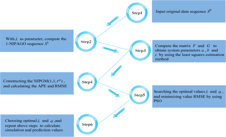
Figure 3: Calculation steps for the NIPGM $(1,1,{{t}^{\alpha}})$ model.

3.3 Optimization step of parameters

Kennedy & Eberhart [1995] developed the particle swarm optimization (PSO) algorithm that originated from the study of the behavior of bird predators. This algorithm has many advantages, such as easy implementation, high precision, and rapid convergence. It has paid close attention to a large number of scholars and applied to many engineering fields [Zeng & Liu, 2017, Zeng & Li, 2018]. The specific algorithm steps will be given below.

Step 1: Set the parameters of learning factor ${{c}_{1}},{{c}_{2}}$, the weight of inertia ${{w}_{\min}}$, ${{w}_{\max}}$, and the maximum number of iterations ${{\rm iter}_{\max}}$.

Step 2: Initialize the particle swarm. Suppose that in an $D$-dimensional target space, there are $n$ candidate particles. The initial position $P_{i}$ and velocity $V_{i}$ of the $i$th particle are $P_{i}=\left(P_{i1},P_{i2},\ldots,P_{iD}\right),$ $V_{i}=\left(V_{i1},V_{i2},\ldots,V_{iD}\right),i\in 1,2,3,\ldots,n$, respectively.

Step 3: Compute the values of fitness ${\rm RMSE}_{i}^{k}$ of each particle. Because the sum of $P_{i}$ and $V_{i}$ is not necessarily limited to the search space, some particles may exceed the edge of the search space during the particle swarm search process. In order to settle this issue, we suppose that the penalty factor $M$ is an arbitrarily large constant and the penalty coefficient $C_{j}$ is used to determine whether the particle exceeds the limit value. If the optimal parameter exceeds the limit value, then $C_{j}=1$, else $C_{j}=0$, there is

$$C_{j}=\left\{\begin{array}[]{ll}{1,}&{\text{ parameter exceeds the limit value }}\\ {0,}&{\text{ others }}\end{array}\right.$$ (45)

Therefore, the fitness of each particle is as follows:

$${\rm RMSE}_{i}^{k}={\rm RMSE}\left(P_{ij}^{k}\right)+\sum_{j=1}^{D}C_{j}M,\quad i\in 1,2,3,\ldots,n,\quad j\in 1,2,3,\ldots,D,$$ (46)

where, $k$ presents current iteration.

Step 4: Update ${\rm pbest}$ and ${\rm globebest}$. According to the fitness ${\rm RMSE}_{i}^{k}$ of each particle, finding out the best position it experiences ${{b}_{k}}$, the individual extremum is recorded as $pbset_{i}={{b}_{k}}$. The optimal position of the entire particle swarm is the global extremum, which recorded as ${\rm globebest}=P_{b_{k}}^{k}$.

(1)If ${\rm RMSE}_{i}^{k+1}<{\rm RMSE}_{i}^{k}$, then ${\rm pbest}_{i}^{k+1}=P_{i}^{k+1}$, else ${\rm pbest}_{i}^{k+1}={\rm pbest}_{i}^{k}$, and find the optimal particle record as ${{b}_{k+1}}$.

(2)If ${\rm RMSE}_{{{b}_{k+1}}}^{k+1}<{\rm RMSE}_{{{b}_{k}}}^{k}$, then ${\rm globebest}^{k+1}={\rm pbest}_{{{b}_{k+1}}}^{k+1}$, else ${\rm globebest}^{k+1}={\rm globebest}^{k}$.

Step 5: Update $V_{ij}^{k+1}$ and $P_{ij}^{k+1}$ according to the following mathematical expression:

$$V_{ij}^{k+1}=V_{ij}^{k}\times w+c_{1}\times rand()\times\left({\rm pbest}_{ij}^{k}-P_{ij}^{k}\right)+c_{2}\times rand()\times\left({\rm globebest}_{j}^{k}-P_{ij}^{k}\right),$$ (47)

$$P_{ij}^{k+1}=V_{ij}^{k+1}+P_{ij}^{k},$$ (48)

$$w=w_{\max}-\frac{w_{\max}-w_{\min}}{{\rm iter}_{\max}}\times k,$$ (49)

where, the inertia weight $w$ is in the interval $\left({{w}_{\min}},{{w}_{\max}}\right)$, ${{c}_{1}}$ and ${{c}_{2}}$ are constant, and the symbol $rand()$ generates random number in $[0,1]$.

Step 6: Stop the guidelines. If $k<{{\rm iter}_{\max}}$, continue to iterate back to step 3, else print optimum solution.

4 Validation of the NIPGM$(1,1,{{t}^{\alpha}})$ model

We present three real examples to examine the accuracy of the novel model, the prediction results are compared with four current grey forecasting models that are classical GM(1, 1)model, discrete DGM (1, 1)model, NGM(1, 1, $k$, $c)$ model, and GM(1, 1, ${{t}^{\alpha}})$ model. Besides, we further assess the prediction accuracy of the novel model by comparing with other famous forecasting models including polynomial regression model (PR)[Zhou, 2018], autoregressive integrated moving average model (ARIMA)[Jiang et al., 2018]. In the PR$(n)$ model, “$n$” is the number of polynomial regressions. In the ARIMA($p,d,q$)model, “$p$ ” presents the number of autoregressive terms, “$d$ ” presents the order of differences, and “$q$ ” presents the number of moving averages.

The unknown parameter $\lambda$ of grey model with time power and parameters $\lambda$, $\alpha$ of the proposed model are determined through the PSO algorithm. Table 1 gives the various parameters setting of the particle swarm algorithm. The computational results of the model optimization parameters $\lambda$, $\alpha$, and RMSE are stored in a matrix with a dimension of $100\times 1000$. Because each trail has an optimal value of $\lambda$, $\alpha$, and RMSE, there are 100 optimal values of $\lambda$, $\alpha$, and RMSE. In this paper, the minimum RMSE and corresponding $\lambda$ and $\alpha$ of the 100 parameters are selected as the system parameters of the model.

Table 1: The parameters setting of PSO algorithm

$c_{1}$ $c_{2}$ $w$ $n$ ${{\rm iter}_{\max}}$ $M$ 2 2 0.6 100 1000 10000

4.1 Case1: Forecasting energy consumption of Jiangsu province

The testing data is derived from the literature[Zhou et al., 2017] in this case. We use scientific computing software Matlab to calculate 100 identical trails, and the numerical results are displayed in Table 2. We see that the minimum values for RMSE and the relevant $\alpha$ of the GM(1, 1, ${{t}^{\alpha}})$ model are 4.2431%, 4.7427, the minimum values for RMSE and the corresponding $\lambda$ and $\alpha$ of NIPGM$(1,1,{{t}^{\alpha}})$ model are 0.012%, 0.3583, 0.6157, respectively.

Table 2: The optimal parameters values of GM(1, 1, ${{t}^{\alpha}})$ model and the novel model in energy consumption of Jiangsu Province.

NIPGM(1, 1, ${{t}^{\alpha}})$ GM(1, 1, ${{t}^{\alpha}})$ RMSE(%) $\lambda$ $\alpha$ RMSE(%) $\alpha$ 0.0120 0.3583 0.6157 4.2431 4.7427

The prediction values of the NIPGM$(1,1,{{t}^{\alpha}})$ and GM$(1,1,{{t}^{\alpha}})$ can be immediately obtained when determining the optimal parameters. Then, we calculate all the numerical results of seven models by using Matlab software, which are displayed in Table 3 and Table 4.

Table 3: The fitted and predicted values for different models in energy consumption of Jiangsu Province(10000 tons of standard coal).

Year value PR(2) ARIMA(2, 1, 0) GM(1, 1) DGM(1, 1) NGM(1, 1, $k$, $c)$ GM(1, 1, ${{t}^{\alpha}})$ NIPGM(1, 1, ${{t}^{\alpha}})$ 2001 8881 8224.8818 8881.0000 8881.0000 8881.0000 8881.0000 8881.0000 8881.0000 2002 9593 10258.6212 9593.0000 11349.6361 11361.2997 9622.0537 10277.1738 9590.5191 2003 11950 12275.3682 11950.0000 12644.2775 12658.6033 11984.7933 11948.6092 11949.8220 2004 14207 14275.1227 14206.9611 14086.5972 14104.0410 14238.3553 13860.9157 14204.8033 2005 16360 16257.8848 16359.2587 15693.4409 15714.5278 16387.7846 16008.5593 16357.5988 2006 18412 18223.6545 18413.0391 17483.5756 17508.9100 18437.8931 18356.5814 18411.1219 2007 20369 20172.4318 20368.7184 19477.9090 19508.1858 20393.2700 20829.7995 20369.0361 2008 22235 22104.2167 22235.1366 21699.7341 21735.7513 22258.2928 23300.5917 22235.4601 2009 24010 24019.0091 24014.3595 24175.0005 24217.6741 24037.1366 25574.9477 24014.7434 2010 25711 25916.8091 25702.5611 26932.6180 26982.9982 25733.7834 27376.4503 25711.3159 2011 27329 27797.6167 27333.0685 30004.7940 30064.0841 27352.0316 28327.8106 27329.5865 2012 28872 29661.4318 28871.8526 33427.4100 33496.9875 28895.5037 27929.5304 28873.8775

It is easy to see in Table 4 that the RMSEPR of ARIMA(2,1,0) model is 0.0127. However, it is noteworthy that the RMSEPO, RMSE of NIPGM (1,1,${{t}^{\alpha}}$) model are 0.0048,0.0120. The numerical results demonstrate that grey NIPGM (1,1,${{t}^{\alpha}}$) model has the highest forecasting accuracy in seven forecasting models. The reason is that the growth of the sequence shows a trend of slowing down and then accelerating, which conforms to the characteristics of the new information priority accumulation. Therefore, using the proposed model to simulate and predict this sequence has higher prediction accuracy.

Table 4: Errors of different models in energy consumption of Jiangsu Province(%).

Year PR(2) ARIMA(2, 1, 0) GM(1, 1) DGM(1, 1) NGM(1, 1, $k$, $c)$ GM(1, 1, ${{t}^{\alpha}})$ NIPGM(1, 1, ${{t}^{\alpha}})$ 2001 7.3879 0.0000 0.0000 0.0000 0.0000 0.0000 0.0000 2002 6.9386 0.0000 18.3116 18.4332 0.3029 7.1320 0.0259 2003 2.7227 0.0000 5.8099 5.9297 0.2912 0.0116 0.0015 2004 0.4795 0.0003 0.8475 0.7247 0.2207 2.4360 0.0155 2005 0.6242 0.0045 4.0743 3.9454 0.1698 2.1482 0.0147 2006 1.0229 0.0056 5.0425 4.9049 0.1406 0.3010 0.0048 2007 0.9650 0.0014 4.3747 4.2261 0.1192 2.2623 0.0002 2008 0.5882 0.0006 2.4073 2.2453 0.1048 4.7924 0.0021 2009 0.0375 0.0182 0.6872 0.8649 0.1130 6.5179 0.0198 2010 0.8005 0.0328 4.7513 4.9473 0.0886 6.4776 0.0012 2011 1.7147 0.0149 9.7910 10.0080 0.0843 3.6548 0.0021 2012 2.7342 0.0005 15.7780 16.0189 0.0814 3.2643 0.0065 RMSEPR 2.5635 0.0127 7.1476 7.1742 0.1885 4.3974 0.0131 RMSEPO 2.2821 0.0105 13.1303 13.3560 0.0829 3.4650 0.0048 RMSE 2.5147 0.0124 8.5525 8.6339 0.1741 4.2431 0.0120

4.2 Case2: Forecasting the output values of the high technology industry

The sample data is taken from the literature[Ding et al., 2017] in this case. Firstly, establishing the grey prediction model by using the data from 2005 to 2012 and testing the forecasting accuracy of grey models by using the data from 2013 to 2014. Then, we calculate 100 identical trails by using Matlab software, and Table 5 gives the optimal numerical results. As can be observed from Table 5, the minimum values for RMSE and the relevant $\alpha$ of grey model with time power are 3.7990%, and 1.7464. The minimum values for RMSE and the relevant $\lambda$ and $\alpha$ of NIPGM(1, 1, ${{t}^{\alpha}})$ model are 3.3509%, 0.9741 and 1.6850, respectively.

Table 5: The optimal parameters values of GM(1, 1, ${{t}^{\alpha}})$ model and the novel model in the output values of the high technology industry.

NIPGM(1, 1, ${{t}^{\alpha}})$ GM(1, 1, ${{t}^{\alpha}})$ RMSE(%) $\lambda$ $\alpha$ RMSE(%) $\alpha$ 3.3509 0.9741 1.6850 3.7990 1.7464

Once the optimal parameters are derived, the numerical results of the grey model with time power and the novel model can be directly calculated. Table 6 and Table 7 list the calculation results of seven models. We can observe from Table 7, the RMSEPR of the extended non-homogeneous exponential grey model is 2.8812, and the RMSEPO, RMSE of the new model are 2.4994, 3.3509. The numerical results reveal that the novel model has more excellent forecasting capability than other prediction models. The reason is that the growing tendency of the sequence shows a trend of acceleration, then deceleration, and acceleration again, has great volatility and conforms to the characteristics of the new information prioritized. Furthermore, only 10 data with non-stationary may be the reason that the PR($n$) model and ARIMA($p,d,q$) model have worse prediction results. So using the NIPGM$(1,1,{{t}^{\alpha}})$ model to stimulate and predict this sequence has higher prediction accuracy.

Table 6: The fitted and predicted values of different models in the output values of the high technology industry(One trillion yuan).

Year value PR(2) ARIMA(1, 1, 1) GM(1, 1) DGM(1, 1) NGM(1, 1, $k$, $c)$ GM(1, 1, ${{t}^{\alpha}})$ NIPGM(1, 1, ${{t}^{\alpha}})$ 2005 3.39 3.5883 3.3900 3.3900 3.3900 3.3900 3.3900 3.3900 2006 4.16 4.0483 4.1346 4.0566 4.0650 4.2669 4.0401 4.1934 2007 4.97 4.6671 4.9564 4.7205 4.7317 4.7987 4.6819 4.7482 2008 5.57 5.4448 5.8125 5.4932 5.5077 5.4628 5.4379 5.5057 2009 5.96 6.3812 6.2863 6.3922 6.4111 6.2920 6.3226 6.4382 2010 7.45 7.4764 6.4872 7.4385 7.4626 7.3276 7.3535 7.5267 2011 8.75 8.7305 8.6574 8.6560 8.6866 8.6209 8.5505 8.7567 2012 10.23 10.1433 10.0763 10.0727 10.1113 10.2358 9.9369 10.1168 2013 11.60 11.7150 11.7224 11.7214 11.7697 12.2525 11.5393 11.5974 2014 12.74 13.4455 13.0781 13.6399 13.7000 14.7710 13.3884 13.1903

Table 7: Errors of different models in the output values of the high technology industry(%).

Year PR(2) ARIMA(1, 1, 1) GM(1, 1) DGM(1, 1) NGM(1, 1, $k$, $c)$ GM(1, 1, ${{t}^{\alpha}})$ NIPGM(1, 1, ${{t}^{\alpha}})$ 2005 5.8505 0.0000 0.0000 0.0000 0.0000 0.0000 0.0000 2006 2.6843 0.6100 2.4864 2.2845 2.5706 2.8812 0.8037 2007 6.0937 0.2743 5.0197 4.7952 3.4465 5.7974 4.4626 2008 2.2484 4.3538 1.3797 1.1178 1.9251 2.3725 1.1541 2009 7.0670 5.4752 7.2524 7.5685 5.5713 6.0843 8.0236 2010 0.3547 12.9233 0.1545 0.1689 1.6425 1.2957 1.0293 2011 0.2231 1.0587 1.0745 0.7251 1.4759 2.2802 0.0768 2012 0.8472 1.5021 1.5371 1.1607 0.0568 2.8655 1.1065 2013 0.9914 1.0550 1.0466 1.4625 5.6253 0.5234 0.0227 2014 5.5375 2.6538 7.0636 7.5356 15.9419 5.0893 3.5346 RMSEPR 3.7840 5.6032 3.5741 3.5586 2.8812 3.7730 3.5569 RMSEPO 3.9779 3.0643 5.0492 5.4279 11.9538 3.6176 2.4994 RMSE 3.8279 5.0324 3.9498 4.0493 6.1815 3.7390 3.3509

4.3 Case3: Forecasting China’s grain production

The sample data is collected from the literature in this case[Ding et al., 2018]. We build forecasting models by employing the data from 2003 to 2012 and assess the prediction capability by employing the data from 2013 to 2015. Similar to case 1 and case 2, Table 8 displays the optimal numerical results.

Table 8: The optimal parameters values of GM(1, 1, ${{t}^{\alpha}})$ model and the novel model in China’s grain production.

NIPGM(1, 1, ${{t}^{\alpha}})$ GM(1, 1, ${{t}^{\alpha}})$ RMSE(%) $\lambda$ $\alpha$ RMSE(%) $\alpha$ 0.9957 0.8965 0.0045 1.0867 1.1714

Furthermore, Table 9 and Table 10 list all calculation results, we can observe the RMSEPR of the extended non-homogeneous exponential grey model is 0.8371, and the RMSEPO, RMSE of the proposed model are 0.6902, 0.9957. The numerical results reveal that the NIPGM (1, 1,${{t}^{\alpha}}$) model has more accurate stimulation and prediction accuracy. Because the growing tendency of the sequence has great volatility and the sequence has new characteristic behavior.

Table 9: The fitted and predicted values of different models in China’s grain production(10000 tons).

Year value PR(2) ARIMA(2, 1, 1) GM(1, 1) DGM(1, 1) NGM(1, 1, $k$, $c)$ GM(1, 1, ${{t}^{\alpha}})$ NIPGM(1, 1, ${{t}^{\alpha}})$ 2003 43069.50 44309.6857 43069.5000 43069.5000 43069.5000 43069.5000 43069.5000 43069.5000 2004 46946.90 45980.3040 46946.9000 46813.7925 46816.8336 47263.8615 46685.2880 47382.7440 2005 48402.20 47624.1546 48066.8211 48129.9249 48133.1370 48308.5300 47970.6232 47933.2230 2006 49804.20 49241.2375 49803.3114 49483.0592 49486.4496 49450.0971 49305.8670 49167.2512 2007 50160.28 50831.5528 51210.9062 50874.2359 50877.8119 50697.5506 50686.0227 50631.5469 2008 52870.92 52395.1004 51688.5287 52304.5244 52308.2939 52060.7120 52108.7434 52179.9439 2009 53082.08 53931.8804 54124.0336 53775.0243 53778.9953 53550.3139 53572.8101 53748.7258 2010 54647.71 55441.8927 54625.9259 55286.8661 55291.0470 55178.0842 55077.6047 55305.8171 2011 57120.80 56925.1374 56033.2806 56841.2122 56845.6116 56956.8388 56622.8742 56833.7626 2012 58957.97 58381.6145 58399.7137 58439.2575 58443.8843 58900.5823 58208.6070 58322.6967 2013 60193.84 59811.3238 60310.0801 60082.2305 60087.0942 61024.6184 59834.9627 59767.0199 2014 60702.60 61214.2656 61615.3786 61771.3944 61776.5046 63345.6700 61502.2275 61163.6716 2015 62143.90 62590.4396 62208.5203 63508.0478 63513.4145 65882.0115 63210.7865 62511.1658

Table 10: The errors of China’s grain production by different models(%).

Year PR(2) ARIMA(2, 1, 1) GM(1, 1) DGM(1, 1) NGM(1, 1, $k$, $c)$ GM(1, 1, ${{t}^{\alpha}})$ NIPGM(1, 1, ${{t}^{\alpha}})$ 2003 2.8795 0.0000 0.0000 0.0000 0.0000 0.0000 0.0000 2004 2.0589 0.0000 0.2835 0.2771 0.6751 0.5573 0.9284 2005 1.6075 0.6929 0.5625 0.5559 0.1935 0.8916 0.9689 2006 1.1304 0.0018 0.6448 0.6380 0.7110 1.0006 1.2789 2007 1.3383 2.0945 1.4233 1.4305 1.0711 1.0481 0.9395 2008 0.9000 2.2364 1.0713 1.0642 1.5324 1.4416 1.3069 2009 0.6009 1.9629 1.3054 1.3129 0.8821 0.9245 1.2559 2010 1.4533 0.0399 1.1696 1.1772 0.9705 0.7867 1.2043 2011 0.3425 1.9039 0.4895 0.4818 0.2870 0.8717 0.5025 2012 0.9776 0.9469 0.8798 0.8720 0.0973 1.2710 1.0775 2013 0.6355 0.1931 0.1854 0.1773 1.3802 0.5962 0.7091 2014 0.8429 1.5037 1.7607 1.7691 4.3541 1.3173 0.7596 2015 0.7186 0.1040 2.1951 2.2038 6.0153 1.7168 0.5910 RMSEPR 1.3519 1.4238 0.9470 0.9471 0.8371 1.0073 1.0785 RMSEPO 0.7373 0.8773 1.6282 1.6348 4.3607 1.2959 0.6902 RMSE 1.2275 1.3087 1.1556 1.1580 2.2977 1.0867 0.9957

4.4 Summary of the case studies

Based on the results of the three case studies, we summarize the performance of simulation and prediction through seven forecasting models. Table 11 gives the average values and ranks of RMSEPR, RMSEPO, and RMSE for seven models in all the cases. It is easy to see that the improved grey model outperforms other models and has better generalization capabilities.

Table 11: The average values and ranks of RMSEPR, RMSEPO and RMSE for seven models in all the cases.

PR($n$) ARIMA($p$,$d$,$q$) GM(1, 1) DGM(1, 1) NGM(1, 1, $k$, $c)$ GM(1, 1, ${{t}^{\alpha}})$ NIPGM(1, 1, ${{t}^{\alpha}})$ Average RMSEPR 2.5665 2.3466 3.8896 3.8933 1.3023 3.0592 1.5495 Simulation rank 4 3 6 7 1 5 2 Average RMSEPO 2.3324 1.3174 6.6026 6.8062 5.4658 0.7929 1.0648 Prediction rank 3 2 6 7 5 4 1 Average RMSE 2.5234 2.1178 4.5527 4.6137 2.8844 3.0229 1.4529 Overall rank 3 2 6 7 4 5 1

On the one hand, the proposed model is compared with PR($n$) model and ARIMA($p,d,q$) model. It reveals that NIPGM(1, 1, ${{t}^{\alpha}})$ model has the most excellent capabilities of simulation and forecasting and has significant advantages for small samples. The reason is that the ARIMA model requires extensive samples of more than 50 observations for prediction [Shumway & Stoffer, 2017]. On the other hand, the RMSE of the NIPGM$(1,1,{{t}^{\alpha}})$ model has been dramatically improved than the basic grey model and discrete grey model. The result indicates that the introduction of the parameters $\alpha$ and $\lambda$ into the grey model is a scientific and practical approach to heighten the forecasting capability of grey forecasting models. Then, we compare the accuracy of the NGM(1, 1, $k$, $c$) model, GM(1, 1, ${{t}^{\alpha}})$ model and novel grey model, which shows that new grey model has the highest prediction accuracy and the second-highest simulation accuracy. This illustrates the importance of new information priority accumulation for forecasting, and grey model with time power and non-homogeneous exponential grey model are particular cases of the proposed model. Besides, the PSO algorithm is very stable when determining the parameters $\lambda$ and $\alpha$. This is why we select the PSO to seek the optimal parameters of the new grey model.

5 Applications in the wind turbine capacity

This section discusses the wind turbine capacity of the world and the top three regions, which are Asia, Europe, and North America, respectively. First of all, Table 12 lists the data of the wind turbine capacity from 2007 to 2017, which gathers from the Statistical Review of World Energy 2018. Secondly, the data is split into two parts, the data from 2007 to 2014 is used to build the PR($n$) model, time series model, and five grey models, including GM(1, 1) model, DGM (1, 1) model, NGM(1, 1, $k)$ model, GM(1, 1, ${{t}^{\alpha}})$ model, and NIPGM(1, 1, ${{t}^{\alpha}})$ model. Thirdly, the data from 2015 to 2017 is applied to assess the capability of the fitting and forecasting. Then, we use Matlab software to compute results. Finally, Fig. 4 displays the structure chart of forecasting the wind turbine capacity, which is drawn under the inspiration of literature[Ma et al., 2019a, Du et al., 2019].

Table 12: The total wind turbine capacity of Europe, North America, Asia, and the world(Megawatts).

Year Europe North America Asia World 2007 56748.8850 18810.0000 15327.3260 91894.0080 2008 64943.4830 27940.0000 22356.3570 116511.6230 2009 77019.9934 38933.0000 33737.5070 151655.8934 2010 86721.9742 45054.0000 48622.3270 182901.3012 2011 96603.1278 53485.0000 69073.8140 222516.8618 2012 109884.8729 67934.0000 87572.6850 269853.3279 2013 120994.6758 71093.0000 105496.3320 303112.5198 2014 133915.4447 78340.0000 129273.7820 351617.6747 2015 147637.6457 87058.4200 167528.3270 417144.1127 2016 161939.8681 96994.0000 189684.6370 467698.4951 2017 178314.1463 104070.0000 209977.2340 514798.1313

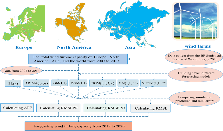
Figure 4: The structure chart of forecasting wind turbine capacity.

5.1 Total wind turbine capacity of Europe

This subsection analyzes the total wind turbine capacity of Europe through seven prediction models. First of all, through the demonstration in section 4, we use PSO algorithm to find the minimum RMSE and the corresponding $\lambda$, $\alpha$ of NIPGM $(1,1,{{t}^{\alpha}})$ model, the smallest RMSE and the corresponding $\alpha$ of grey model with time power. Then, Table 13 displays the minimum RMSE and the relevant optimal values of the two models.

Table 13: The optimal parameters values of GM(1, 1, ${{t}^{\alpha}})$ model and the novel model in wind turbine capacity of Europe.

NIPGM(1, 1, ${{t}^{\alpha}})$ GM(1, 1, ${{t}^{\alpha}})$ RMSE(%) $\lambda$ $\alpha$ RMSE(%) $\alpha$ 0.3799 0.9649 0.0206 1.6360 3.6598

Further, five grey models are respectively constructed by using grey theory and the row data of the wind turbine capacity from 2007 to 2014.

$\bullet$ GM(1, 1) model

We can immediately get $(a,b)=(-0.1148,57660.2383)$ of the basic grey model by using the least-squares method. Thus the whitening equation is established, there is

$$\frac{ds_{t}^{1}}{dt}-0.1148s_{t}^{1}=57660.2383.$$ (50)

$\bullet$ DGM(1, 1) model

We can get $({{\beta}_{1}},{{\beta}_{2}})=(1.1218,61171.4813)$ of DGM (1, 1)model. Then the time response sequence is obtained, these is

$$\hat{s}_{k}^{1}=1.1218^{k}s_{k}^{0}-\frac{1-1.1218^{k}}{0.1218}\times 61171.4813,k=1,2,\cdots,m.$$ (51)

$\bullet$ NGM(1, 1, $k$, $c)$ model

We directly derive $(a,b,c)=(-0.0384,7583.1441$,$50768.5848)$ of the extended non-homogeneous exponential grey model. And the whitening equation is established, then

$$\frac{ds_{t}^{1}}{dt}-0.0384s_{t}^{1}=7583.1441t+50768.5848.$$ (52)

$\bullet$ GM$(1,1,{{t}^{\alpha}})$ model

We can observe from Table 13 that the optimal parameter $\alpha=3.6598$ of grey model with time power. And applying the least-squares method, we can get $(a,b,c)=(-0.1396,-7.4040,53659.7544)$. Thus, the whitening equation is put forward, there is

$$\frac{ds_{t}^{1}}{dt}-0.1396s_{t}^{1}=-7.4040t^{3.6598}+53659.7544.$$ (53)

$\bullet$ NIPGM$(1,1,{{t}^{\alpha}})$ model

Similar to grey GM$(1,1,{{t}^{\alpha}})$ model, $\lambda=0.9649$ and $\alpha=0.0206$ of NIPGM$(1,1,{{t}^{\alpha}})$ model are also obtained. Thus, the one-time new information priority accumulated generation operation sequence(1-NIPAGO) can be expressed as follow.

$$s_{k}^{1}=\sum_{v=1}^{k}0.9649^{k-v}s_{v}^{0},k=1,2,\cdots,m.$$

Then, the new information priority accumulation sequence $S^{1}$ and the matrix $F,G$ are given as follows.

$${S^{1}}=\left(\begin{array}[]{*{35}{r}}56748.8850\\ 119703.1115\\ 192527.0720\\ 272500.2666\\ 359551.2611\\ 456832.5442\\ 561813.5647\\ 676035.3844\\ \end{array}\right),F=\left(\begin{array}[]{*{35}{r}}-88225.9983&1.0080&1\\ -156115.0918&1.0190&1\\ -232513.6693&1.0261&1\\ -316025.7638&1.0315&1\\ -408191.9027&1.0358&1\\ -509323.0545&1.0394&1\\ -618924.4745&1.0425&1\\ \end{array}\right),G=\left(\begin{array}[]{*{35}{r}}62954.2265\\ 72823.9605\\ 79973.1945\\ 87050.9945\\ 97281.2831\\ 104981.0205\\ 114221.8197\\ \end{array}\right).$$

Finally, the optimal parameters $(a,b,c)=(-0.0737,-345863.1636,-291896.7690)$ of NIPGM$(1,1,{{t}^{\alpha}})$ model are obtained. And the whitening equation is given, these is

$$\frac{ds_{t}^{1}}{dt}-0.0737s_{t}^{1}=-345863.1636t^{0.0206}-291896.7690.$$ (54)

The prediction values of the seven models in the wind turbine capacity of Europe are listed in Table 14. It is seen from Table 14 and Fig. 5 that the established forecasting model can reflect the trend of wind turbine capacity in Europe from 2015 to 2017.

Table 14: The fitted and predicted values of different models in wind turbine capacity of Europe(Megawatts).

Year data PR(3) ARIMA(2, 1, 1) GM(1, 1) DGM(1, 1) NGM(1, 1, $k$, $c)$ GM(1, 1, ${{t}^{\alpha}})$ NIPGM(1, 1, ${{t}^{\alpha}})$ 2007 56748.8850 56446.3721 56748.8850 56748.8850 56748.8850 56748.8850 56748.8850 56748.8850 2008 64943.4830 65969.7452 64943.4830 68007.2739 68086.5467 65502.2396 66034.0365 64985.6025 2009 77019.9934 75999.9366 75106.1003 76283.1268 76381.7043 75799.3255 75715.7796 76166.9682 2010 86721.9742 86540.1637 86607.7451 85566.0740 85687.4822 86499.7040 86488.2844 86832.2696 2011 96603.1278 97593.6435 98309.8152 95978.6696 96127.0068 97619.1706 98253.2028 97720.3058 2012 109884.8729 109163.5934 108836.2802 107658.3813 107838.4052 109174.1390 110841.1855 109111.8638 2013 120994.6758 121253.2304 121799.3639 120759.4053 120976.6332 121181.6661 124006.1529 121167.8665 2014 133915.4447 133865.7719 134856.0580 135454.7021 135715.5250 133659.4765 137417.3283 134005.8885 2015 147637.6457 147004.4350 147994.4670 151938.2798 152250.0937 146625.9893 150649.2690 147726.0120 2016 161939.8681 160672.4369 162535.6398 170427.7558 170799.1109 160100.3448 163169.8761 162421.7532 2017 178314.1463 174872.9948 177791.4872 191167.2290 191608.0023 174102.4332 174326.2387 178185.4696

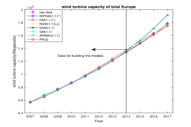
Figure 5: The fitted and predicted values of different models in wind turbine capacity of Europe.

The values of APE, RMSEPR, RMSEPO, and RMSE are calculated according to Eq.(32) to Eq.(34), and Table 15 gives all the results. Besides, Fig. 6(left) presents the absolute percentage errors and Fig. 6(right) provides the comparison results of RMSEPO and RMSE. It is easy observed from Table 15 and Fig.6 that the RMSEPR, RMSEPO, and RMSE of NIPGM$(1,1,{{t}^{\alpha}})$ are 0.4815, 0.1432, 0.3799, respectively. The results display that the novel model has the most beneficial fitting and forecasting capabilities than other models, which explains the importance of new information priority accumulated to predicting.

Table 15: Errors of different models in wind turbine capacity of Europe(%).

Year PR(3) ARIMA(2, 1, 1) GM(1, 1) DGM(1, 1) NGM(1, 1, $k$, $c)$ GM(1, 1, ${{t}^{\alpha}})$ NIPGM(1, 1, ${{t}^{\alpha}})$ 2007 0.5331 0.0000 0.0000 0.0000 0.0000 0.0000 0.0000 2008 1.5802 0.0000 4.7176 4.8397 0.8604 1.6792 0.0649 2009 1.3244 2.4849 0.9567 0.8287 1.5849 1.6933 1.1075 2010 0.2096 0.1317 1.3329 1.1929 0.2563 0.2695 0.1272 2011 1.0253 1.7667 0.6464 0.4929 1.0518 1.7081 1.1565 2012 0.6564 0.9543 2.0262 1.8624 0.6468 0.8703 0.7035 2013 0.2137 0.6651 0.1944 0.0149 0.1545 2.4889 0.1431 2014 0.0371 0.7024 1.1494 1.3442 0.1911 2.6150 0.0675 2015 0.4289 0.2417 2.9130 3.1242 0.6852 2.0399 0.0599 2016 0.7827 0.3679 5.2414 5.4707 1.1359 0.7595 0.2976 2017 1.9298 0.2931 7.2081 7.4553 2.3620 2.2365 0.0722 RMSEPR 0.7210 0.9579 1.5748 1.5108 0.6780 1.6178 0.4815 RMSEPO 1.0471 0.3009 5.1208 5.3501 1.3944 1.6786 0.1432 RMSE 0.8188 0.7608 2.6386 2.6626 0.8929 1.6360 0.3800

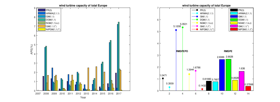
Figure 6: Errors of different models in wind turbine capacity of Europe.

5.2 Total wind turbine capacity of North America

In this subsection, the total wind turbine capacity in North America is studied by seven forecasting models. Similar to the analysis in section 4, Table 16 lists the minimum RMSE and the corresponding optimized parameters of the two models.

Table 16: The optimal parameters values of GM(1, 1, ${{t}^{\alpha}})$ model and the novel model in total wind turbine capacity of North America.

NIPGM(1, 1, ${{t}^{\alpha}})$ GM(1, 1, ${{t}^{\alpha}})$ RMSE(%) $\lambda$ $\alpha$ RMSE(%) $\alpha$ 2.4236 0.9086 0.2637 5.4472 1.6400

Further, the forecasting models are built by using the wind turbine capacity data from 2007 to 2014 in North America. Table 17 gives the fitting and predicting values of the seven models. It can be noticed from Fig. 7 and Table 17 that the established seven forecasting models have an excellent predictive effect in wind turbine capacity forecasting of North America, which can reflect the trend of wind turbine capacity from 2015 to 2017.

Table 17: The fitted and predicted values of different models in wind turbine capacity of North America(Megawatts).

Year data PR(1) ARIMA(2, 1, 1) GM(1, 1) DGM(1, 1) NGM(1, 1, $k$, $c)$ GM(1, 1, ${{t}^{\alpha}})$ NIPGM(1, 1, ${{t}^{\alpha}})$ 2007 18810.0000 19869.0833 18810.0000 18810.0000 18810.0000 18810.0000 18810.0000 18810.0000 2008 27940.0000 28534.6667 27940.0000 33430.1116 33498.4981 28055.3165 23953.1486 27265.0412 2009 38933.0000 37200.2500 37524.5787 38866.9876 38957.6409 37830.7879 34862.0700 37921.7659 2010 45054.0000 45865.8333 48161.9090 45188.0851 45306.4426 47064.7950 45973.1476 46970.6018 2011 53485.0000 54531.4167 54092.3164 52537.2085 52689.8882 55787.3295 56359.8353 55366.0191 2012 67934.0000 63197.0000 62249.4276 61081.5500 61276.5902 64026.7220 65947.8132 63448.7993 2013 71093.0000 71862.5833 76226.4435 71015.4928 71262.6395 71809.7338 74849.8077 71379.1940 2014 78340.0000 80528.1667 79298.1398 82565.0334 82876.0831 79161.6438 83193.0517 79243.8894 2015 87058.4200 89193.7500 86307.0648 95992.9231 96382.1325 86106.3307 91081.8126 87093.9468 2016 96994.0000 97859.3333 94743.4150 111604.6455 112089.2193 92666.3508 98595.3608 94961.1729 2017 104070.0000 106524.9167 104358.1253 129755.3663 130356.0397 98863.0108 105793.3036 102866.1383

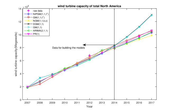
Figure 7: The fitted and predicted values of different models in wind turbine capacity of North America.

According to the Eq.(32) to Eq.(34), the values of fitting and forecasting errors of the seven models can be calculated. Table 18 and Fig.8 show that the RMSEPR, RMSEPO and RMSE of NIPGM$(1,1,{{t}^{\alpha}})$ are 2.9918, 1.0978, 2.4236. The numerical results expose that the forecasting and fitting accuracy of the novel model are higher than other models. And new information priority accumulation has great significance for enhancing the prediction accuracy. Therefore, the proposed model is very suitable for forecasting wind turbine capacity in North America.

Table 18: Errors of different models in wind turbine capacity of North America(%).

Year PR(1) ARIMA(2, 1, 1) GM(1, 1) DGM(1, 1) NGM(1, 1, $k$, $c)$ GM(1, 1, ${{t}^{\alpha}})$ NIPGM(1, 1, ${{t}^{\alpha}})$ 2007 5.6304 0.0000 0.0000 0.0000 0.0000 0.0000 0.0000 2008 2.1284 0.0000 19.6496 19.8944 0.4127 14.2693 2.4157 2009 4.4506 3.6176 0.1696 0.0633 2.8310 10.4562 2.5974 2010 1.8019 6.8982 0.2976 0.5603 4.4631 2.0401 4.2540 2011 1.9565 1.1355 1.7721 1.4866 4.3046 5.3750 3.5169 2012 6.9729 8.3678 10.0869 9.7998 5.7516 2.9237 6.6023 2013 1.0825 7.2207 0.1090 0.2386 1.0082 5.2844 0.4026 2014 2.7932 1.2231 5.3932 5.7903 1.0488 6.1949 1.1538 2015 2.4528 0.8630 10.2627 10.7097 1.0936 4.6215 0.0408 2016 0.8922 2.3203 15.0635 15.5630 4.4618 1.6510 2.0958 2017 2.3589 0.2769 24.6809 25.2580 5.0034 1.6559 1.1568 RMSEPR 3.0266 4.0661 5.3540 5.4048 2.8314 6.6491 2.9918 RMSEPO 1.9013 1.1534 16.6690 17.1769 3.5196 2.6428 1.0978 RMSE 2.6890 3.1923 8.7485 8.9364 3.0379 5.4472 2.4236

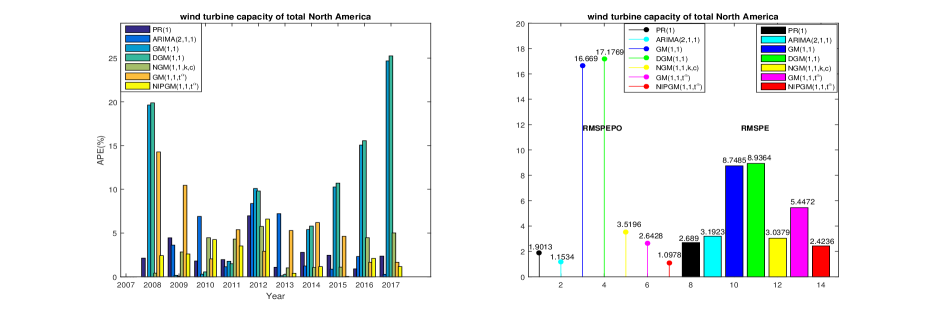
Figure 8: Errors of different models in wind turbine capacity of North America.

5.3 Total wind turbine capacity of Asia

This subsection considers the total wind turbine capacity of Asia through seven forecasting models. According to the discussion in Section 4, the minimum RMSE and corresponding optimal parameters of the two models are listed Table 19.

Table 19: The optimal parameters of GM(1,1,${{t}^{\alpha}})$ model and the novel model in total wind turbine capacity of Asia.

NIPGM(1, 1, ${{t}^{\alpha}})$ GM(1, 1, ${{t}^{\alpha}})$ RMSE(%) $\lambda$ $\alpha$ RMSE(%) $\alpha$ 3.3256 0.9014 1.0978 4.5568 2.1840

Table 20: The fitted and predicted values of different models in wind turbine capacity of Asia(Megawatts).

Year data PR(2) ARIMA(2, 1, 2) GM(1, 1) DGM(1, 1) NGM(1, 1, $k$, $c)$ GM(1, 1, ${{t}^{\alpha}})$ NIPGM(1, 1, ${{t}^{\alpha}})$ 2007 15327.3260 13614.4778 15327.3260 15327.3260 15327.3260 15327.3260 15327.3260 15327.3260 2008 22356.3570 23523.2229 24442.2317 30411.7783 30593.2156 20761.8645 19571.5731 21279.7344 2009 33737.5070 35665.8868 36990.6742 39064.6946 39349.6869 34761.6976 32086.3194 34904.5823 2010 48622.3270 50042.4692 44795.2174 50179.5833 50612.4585 50156.2873 49814.9600 50316.4550 2011 69073.8140 66652.9702 66555.9999 64456.9375 65098.8905 67084.5888 69887.5839 67445.5987 2012 87572.6850 85497.3899 85642.7395 82796.5584 83731.6674 85699.4005 91305.4153 86273.5270 2013 105496.3320 106575.7282 109051.7419 106354.2630 107697.5672 106168.7439 113672.2917 106801.6654 2014 129273.7820 129887.9851 124833.1761 136614.7274 138523.0502 128677.3797 136798.4924 129041.2131 2015 167528.3270 155434.1606 156064.2433 175485.0554 178171.4847 153428.4759 160573.3168 153008.8500 2016 189684.6370 183214.2548 194671.4654 225414.9700 229168.1992 180645.4414 184921.4951 178724.6215 2017 209977.2340 213228.2675 217864.4953 289551.2019 294761.3285 210573.9425 209786.6733 206210.7892

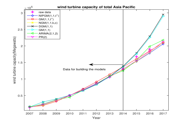
Figure 9: The fitted and predicted values of different models in wind turbine capacity of Asia.

Table 21: Errors of different models in wind turbine capacity of Asia(%).

Year PR(2) ARIMA(2, 1, 2) GM(1, 1) DGM(1, 1) NGM(1, 1, $k$, $c)$ GM(1, 1, ${{t}^{\alpha}})$ NIPGM(1, 1, ${{t}^{\alpha}})$ 2007 11.1751 0.0000 0.0000 0.0000 0.0000 0.0000 0.0000 2008 5.2194 9.3301 36.0319 36.8435 7.1322 12.4563 4.8157 2009 5.7158 9.6426 15.7901 16.6348 3.0358 4.8942 3.4593 2010 2.9208 7.8711 3.2028 4.0930 3.1548 2.4529 3.4843 2011 3.5047 3.6451 6.6840 5.7546 2.8799 1.1781 2.3572 2012 2.3698 2.2038 5.4539 4.3861 2.1391 4.2624 1.4835 2013 1.0232 3.3702 0.8132 2.0866 0.6374 7.7500 1.2373 2014 0.4751 3.4350 5.6786 7.1548 0.4613 5.8208 0.1799 2015 7.2192 6.8431 4.7495 6.3530 8.4164 4.1515 8.6669 2016 3.4111 4.6528 18.8367 20.8154 4.7654 2.5111 5.7780 2017 1.5483 3.7562 37.8965 40.3778 0.2842 0.0908 1.7937 RMSEPR 3.0327 5.6426 10.5221 10.9933 2.7772 5.5450 2.4310 RMSEPO 4.0595 5.0841 20.4942 22.5154 4.4887 2.2511 5.4129 RMSE 3.3407 5.4750 13.5137 14.4500 3.2906 4.5568 3.3256

Table 20 and Fig. 9 display the simulation and prediction values. Table 21 and Fig. 10 show the results of APE, RMSEPR, RMSEPO, and RMSE. We can notice from Fig.10 and Table 21 that the maximum forecasting error of the basic grey model and discrete grey model are as high as 37.8965%,40.3778%, respectively. It means that the forecasting error of the basic grey model and discrete grey model are enormous. Further, the RMSEPR of the novel model is 2.4310, the RMSEPO of the grey model with time power is 2.2511, and the RMSE of the extended non-homogeneous exponential grey model is 3.2906. The results display that the prediction errors of the novel grey model are smaller than other models. Besides, the grey model with time power and extended non-homogeneous exponential grey model are particular cases of the proposed model. What’s more, it can indicate that the new information prioritization is important for forecasting.

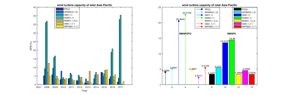
Figure 10: Errors of different models in wind turbine capacity of Asia.

5.4 Total wind turbine capacity of the world

In this subsection, the global wind turbine capacity is derived through seven prediction models. Table 22 lists the minimum RMSE and the corresponding optimal values of the two models.

Table 22: The optimal parameters values of GM(1, 1, ${{t}^{\alpha}})$ model and the novel model in total wind turbine capacity of the world.

NIPGM(1, 1, ${{t}^{\alpha}})$ GM(1, 1, ${{t}^{\alpha}})$ RMSE(%) $\lambda$ $\alpha$ RMSE(%) $\alpha$ 1.4391 0.7161 1.3276 4.0898 2.8605

Table 23: The fitted and predicted values of different models in wind turbine capacity of the world(Megawatts).

Year data PR(2) ARIMA(2, 1, 1) GM(1, 1) DGM(1, 1) NGM(1, 1, $k$, $c)$ GM(1, 1, ${{t}^{\alpha}})$ NIPGM(1, 1, ${{t}^{\alpha}})$ 2007 91894.0080 89895.7940 91894.0080 91894.0080 91894.0080 91894.0080 91894.0080 91894.0080 2008 116511.6230 119032.8856 116511.6230 129789.1184 130130.5184 115887.4467 118956.8735 117442.6582 2009 151655.8934 150938.8752 152167.2895 153837.9115 154305.9948 149773.8023 148814.4211 151376.2996 2010 182901.3012 185613.7630 188450.4898 182342.7364 182972.7593 185600.8220 184697.3033 187037.5395 2011 222516.8618 223057.5489 221338.5422 216129.2570 216965.1975 223479.6474 226537.3484 224763.4997 2012 269853.3279 263270.2329 262789.1973 256176.1257 257272.7062 263527.7848 273643.5552 264896.4706 2013 303112.5198 306251.8150 313238.8541 303643.3302 305068.4908 305869.4703 324527.1561 307861.1290 2014 351617.6747 352002.2953 348668.0199 359905.7943 361743.7133 350636.0549 376684.5272 354209.7165 2015 417144.1127 400521.6737 399131.1492 426593.2028 428947.9839 397966.4121 426326.0794 404666.5259 2016 467698.4951 451809.9502 469387.1588 505637.2072 508637.3755 448007.3685 468036.6722 460180.8872 2017 514798.1313 505867.1249 524331.1065 599327.3771 603131.3573 500914.1595 494349.5839 521994.0838

Furthermore, all the results of seven forecasting models are listed in Table 23, Fig.11, Table 24 and Fig.12. We can observe in Table 24, and Fig.12, the RMSEPR of the extended non-homogeneous exponential grey model is 1.0312. However, it is worth noting that the RMSEPO and RMSE of NIPGM$(1,1,{{t}^{\alpha}})$ are 1.9988, 1.4392, respectively. The results display that the extended non-homogeneous exponential grey model has the best accuracy of fitting and the NIPGM$(1,1,{{t}^{\alpha}})$ has the best performance of forecasting. The reason is that the extended non-homogeneous exponential grey model is a particular case of the proposed model. Thus, the new grey model is suitable for predicting wind turbine capacity in the world.

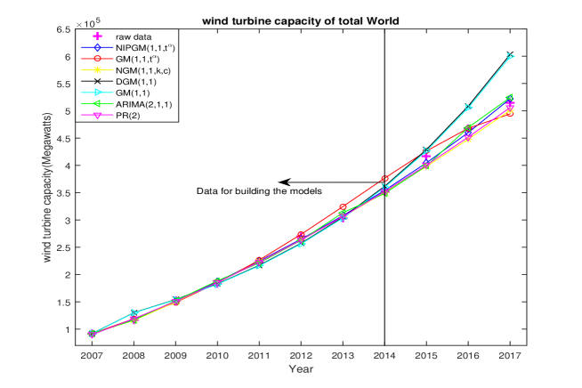
Figure 11: The fitted and predicted values of different models in global wind turbine capacity.

Table 24: Errors of different models in global wind turbine capacity(%).

Year PR(2) ARIMA(2, 1, 1) GM(1, 1) DGM(1, 1) NGM(1, 1, $k$, $c)$ GM(1, 1, ${{t}^{\alpha}})$ NIPGM(1, 1, ${{t}^{\alpha}})$ 2007 2.1745 0.0000 0.0000 0.0000 0.0000 0.0000 0.0000 2008 2.1640 0.0000 11.3959 11.6889 0.5357 2.0987 0.7991 2009 0.4728 0.3372 1.4388 1.7474 1.2410 1.8736 0.1844 2010 1.4830 3.0340 0.3054 0.0391 1.4759 0.9820 2.2615 2011 0.2430 0.5295 2.8706 2.4949 0.4327 1.8068 1.0096 2012 2.4395 2.6178 5.0684 4.6620 2.3441 1.4046 1.8369 2013 1.0357 3.3408 0.1751 0.6453 0.9095 7.0649 1.5666 2014 0.1094 0.8389 2.3571 2.8798 0.2792 7.1290 0.7372 2015 3.9848 4.3182 2.2652 2.8297 4.5974 2.2011 2.9912 2016 3.3972 0.3611 8.1118 8.7533 4.2102 0.0723 1.6074 2017 1.7349 1.8518 16.4199 17.1588 2.6970 3.9721 1.3978 RMSEPR 1.1353 1.5283 3.3730 3.4511 1.0312 3.1942 1.1993 RMSEPO 3.0390 2.1770 8.9323 9.5806 3.8349 2.0819 1.9988 RMSE 1.7064 1.7229 5.0408 5.2899 1.8723 2.8605 1.4392

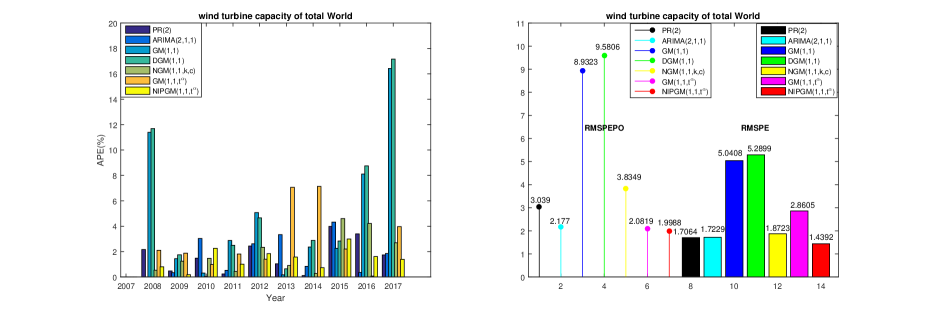
Figure 12: Errors of different models in wind turbine capacity of the world.

5.5 Comparison of prediction models

According to the results of forecasting wind turbine capacity in Europe, North America, Asia, and the world, we further compare the performance of accuracy of seven forecasting models. The ranks of the performance of simulation and prediction are listed in Table 25. As can be observed from Table 25, all the prediction models can get acceptable results by 8 years of wind turbine capacity data. However, it is worth noting that the NIPGM$(1,1,{{t}^{\alpha}})$ model has the best simulation and prediction capability in wind turbine capacity forecasting.

Table 25: The average values and ranks of RMSEPR, RMSEPO and RMSE for seven models in wind turbine capacity forecasting.

PR($n$) ARIMA($p$, $d$, $q$) GM(1, 1) DGM(1, 1) NGM(1, 1, $k$, $c)$ GM(1, 1, ${{t}^{\alpha}})$ NIPGM(1, 1, ${{t}^{\alpha}})$ Average RMSEPR 2.6385 4.0650 6.9413 7.1200 2.4393 5.6687 2.3679 Simulation rank 3 4 6 7 2 5 1 Average RMSEPO 3.3490 2.9051 17.0721 18.2077 4.4125 2.8848 2.8842 Prediction rank 4 3 6 7 5 2 1 Average RMSE 2.8517 3.7170 9.9805 10.4463 3.03123 4.8335 2.5228 Overall rank 2 4 6 7 3 5 1

Among the seven prediction models, both of the polynomial regression model and time series model require a lot of historical data when establishing the prediction model. In wind turbine capacity forecasting, using only 8 data to develop prediction models is the reason of poor prediction accuracy. Compared with several grey models, we find that new information priority accumulation can significantly exploit data with new characteristic behaviors. Therefore, the NIPGM$(1,1,{{t}^{\alpha}})$ model has a great advantage for small samples with new characteristic behaviors.

5.6 Future discussion and development suggestion

As can be seen from the above discussion, the NIPGM$(1,1,{{t}^{\alpha}})$ outperforms other six prediction models. Therefore, the NIPGM$(1,1,{{t}^{\alpha}})$ model will be applied to predict wind turbine capacity of Europe, North America, Asia, and the world from 2018 to 2020. Table 26 and Fig.13 lists the prediction values, and Table 27 displays the annual increase rates.

With the continuous deepening understanding of environmental issues around the world, and the constant improvement of renewable energy comprehensive utilization technologies, the global wind power industry has quickly improved in recent years. At present, wind power generation has turned into one of the fastest-growing renewable energy sources, and its proportion has been increasing in clean energy production. Thus, it owes broad prospects for development. Further, we will present the growth trend of the next three years of wind turbine capacity in Europe, North America, Asia, and the world.

Table 26: The results of the wind turbine capacity in Europe, North America, Asia, and the world from 2017 to 2020(Megawatts).

Year Europe North America Asia World 2017 178314.1463 104070.0000 209977.2340 514798.1313 2018 195111.4074 110822.4755 235491.1594 591725.3917 2019 213297.6361 118839.3441 266590.6714 671483.3296 2020 232847.4225 126922.9203 299535.1338 764009.7685

Table 27: The results of annual increase rate of wind turbine capacity in Europe, North America, Asia, and the world from 2017 to 2020(%).

Year Europe North America Asia World 2017 10.1113 7.2953 10.6981 10.0705 2018 9.4200 6.4884 12.1508 14.9432 2019 9.3209 7.2340 13.2062 13.4789 2020 9.1655 6.8021 12.3577 13.7794 mean value 9.5045 6.9549 12.1032 13.0680

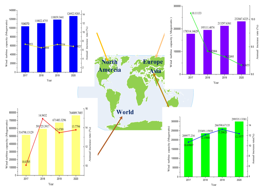
Figure 13: The results of prediction and annual increase rate of wind turbine capacity in Asia ,Europe, North America, and the world from 2017 to 2020.

In Europe, it is predicted that the wind turbine capacity will maintain steady growth at an average annual growth rate of 9.5045% approximately, which will reach 232847.4225 Megawatts in 2020. And the annual increase rate of wind turbine capacity will decline in the next three years. The result is consistent with the predicted result of the GWEC Global Wind Report 2018 (https://gwec.net) and literature[Klessmann et al., 2011]. The reason is that many Member States of US reduce wind turbine capacity investments and support programs. While the wind turbine capacity in Europe is increasing, which will face regional imbalances and bring challenges in materials, control, and storage[Scarlat et al., 2015]. Therefore, it is possible to promote the excellent and rapid advancement of wind power generation in Europe by researching and developing diversified technologies for cleaner production.

In North America, the wind turbine capacity will grow at an average annual increase rate of 6.9549%, and it will increase from 104070 Megawatts in 2017 to 126922.9303 Megawatts in 2020. It reflects that the wind turbine in North America has an unstable growth trend in the future. Although North America has enormous potential for wind energy development, some parts still rely on fossil fuels for power generation[Mercer et al., 2017]. The GWEC Global Wind Report 2018 states that governments’ commitment to large-scale auction is driving the wind turbine capacity. Therefore, governments should maintain their commitment and make reasonable policies to promote positive development.

In Asia, the wind turbine capacity will continue to grow at an average annual increase rate of 12.1032% approximately, which is expected to reach 299535.1338 Megawatts in 2020. As we all know, Asia is the region with the largest installed capacity of global wind turbines. However, the wind energy of South-East Asia and India will remain at a moderate level. Therefore, South-East Asian governments should call for stop prioritizing coal[Shukla et al., 2017]. For example, Vietnam should increase a higher tax on fossil fuel to promote the development of clean energy department[Nong et al., 2019]. India should drive the volume of wind turbine capacity with the execution of the scheduled auctions[Neeru et al., 2019]. Furthermore, the relevant practitioners can use effective wind energy prediction methods to increase wind turbine capacity[Yang et al., 2019]. Besides, Asian governments should correctly recognize the opportunities and challenges for renewable energy and increase cooperation among countries of the renewable energy sector[Sharvini et al., 2018].

In the world, the wind turbine capacity will maintain sharply increase from 514798.1313 Megawatts in 2017 to 764009.7685 Megawatts in 2020, which the average annual growth rate is 13.0068%. Currently, global wind power accounts for 16% of renewable energy[Heuberger & Dowell, 2018]. With the rapid development of wind energy, wind power generation has received more and more attention from all over the world. It is imperative to increase the construction of wind turbines, expand the scale of clean energy supply[Lundie et al., 2019], and promote the continuous improvement of production technology by power generation enterprises. Countries around the world should increase communication and cooperation[Akizu-Gardoki et al., 2018] between the wind power sectors. These suggestions can contribute to advance of the low carbon economy and achieve rapid development of clean energy production.

6 Conclusions

In this paper, combining the new information priority accumulation with grey GM(1, 1, ${{t}^{\alpha}})$ model, we propose a novel NIPGM$(1,1,{{t}^{\alpha}})$ model to predict short-term wind turbine capacity of Europe, North America, Asia, and the world. The NIPGM$(1,1,{t}^{\alpha})$ model is a more generic model. The traditional GM$(1,1)$ model, NGM(1, 1, $k$, $c)$ model, NGM(1, 1, $k)$ model, and GM(1, 1, ${t}^{\alpha})$ model are special cases of the proposed model with determined parameters $\lambda$ and $\alpha$.

Three numerical cases are used to evaluate the accuracy of the novel model and six existing prediction models. It shows that the NIPGM$(1,1,{t}^{\alpha})$ model has a sufficient advantage for small samples than the polynomial regression model and the time series model. Furthermore, the proposed model is superior to other forecasting models, the results reveal that new information priority accumulation is an effective method to improve the prediction ability of grey model. Besides, the particle swarm optimization algorithm is very stable when determining the optimal values of nonlinear parameters.

The proposed model is applied to predict the total wind turbine capacity, and it has the highest simulation and prediction accuracy than other commonly prediction models. It is predicted that the average annual increase rate of the total wind turbine capacity in Europe, North America, Asia, and the world from 2018 to 2020 are 9.5045%, 6.9549%, 12.1032%, 13.0680%, respectively. In the future, wind energy will make an enormous contribution to the sustainable development of cleaner production. Additionally, reasonable suggestions are put forward from the standpoint of the practitioners and governments. (1)The related practitioners can use useful prediction models to predict wind turbine capacity to ensure the installation of wind turbines. And they can strengthen the construction of the wind power system and innovate wind power technology to achieve an efficient configuration of the power supply system and develop economic efficiency. (2)Governments around the world should increase communication and cooperation to promote competition and development in the global energy market. Moreover, governments can make rational policies and increase the cost-effectiveness of renewable energy into the power supply, which can promote the sustainable development of clean energy production in the future.

From the perspective of the new information accumulation, it focuses on mining new information rules, and new information has a more significant impact on the forecasting. Therefore, the grey forecasting model with new information priority accumulation is suitable for the small sample with new characteristic behaviors. It can be applied to the prediction of other cleaner production such as solar and natural gas. In the future, we will combine the new information priority accumulation with other grey models to research whether the prediction accuracy of other grey models would be improved.

References

References

- Akizu-Gardoki et al. [2018] Akizu-Gardoki, O., Bueno, G., Wiedmann, T., Lopez-Guede, J. M., Arto, I., Hernandez, P., & Moran, D. (2018). Decoupling between human development and energy consumption within footprint accounts. Journal of Cleaner Production, 202, 1145 – 1157.
- Chang et al. [2017] Chang, G. W., Lu, H. J., Chang, Y. R., & Lee, Y. D. (2017). An improved neural network-based approach for short-term wind speed and power forecast. Renewable Energy, 105, 301–311.
- Cui et al. [2009] Cui, J., Dang, Y. G., & Liu, S. F. (2009). Novel grey forecasting model and its modeling mechanism. Control & Decision, 24, 1702–1706.
- Deng [1982] Deng, J. L. (1982). Control problems of grey systems. Systems & Control Letters, 1, 288–294.
- Ding et al. [2017] Ding, S., Dang, Y. G., Ning, X. U., Wei, L., & Jing, Y. E. (2017). Multi-variable time-delayed discrete grey model. Control & Decision, 32, 199–202.
- Ding et al. [2018] Ding, S., Dang, Y. G., Ning, X. U., & Zhu, X. Y. (2018). Modeling and applications of DFCGM and its extended model based on driving factors control. Control & Decision, 33, 712–718.
- Du et al. [2019] Du, P., Wang, J. Z., & Niu, T. (2019). A novel hybrid model for short-term wind power forecasting. Applied Soft Computing, 80, 93–106.
- Duan et al. [2019] Duan, H. M., Xiao, X. P., & Xiao, Q. Z. (2019). An inertia grey discrete model and its application in short-term traffic flow prediction and state determination. Neural Computing and Applications, . doi:https://doi.org/10.1007/s00521-019-04364-w.
- Heuberger & Dowell [2018] Heuberger, C. F., & Dowell, N. M. (2018). Real-world challenges with a rapid transition to 100% renewable power systems. Joule, 2, 367 – 370.
- Hu et al. [2009] Hu, R., Zhuang, Q. J., Zhu, L., & Fu, Y. (2009). Application of improved discrete grey model in medium-long term power load forecasting. Journal of Electric Power Science & Technology, 24, 49–53.
- Jiang et al. [2018] Jiang, S. M., Chen, Y., Guo, J. T., & Ding, Z. W. (2018). ARIMA forecasting of China’s coal consumption, price and investment by 2030. Energy Sources Part B Economics Planning & Policy, 13, 1–6.
- Jiang et al. [2012] Jiang, W., Yan, Z., Feng, D. H., & Zhi, H. (2012). Wind speed forecasting using autoregressive moving average/generalized autoregressive conditional heteroscedasticity model. European Transactions on Electrical Power, 22, 662–673.
- Kennedy & Eberhart [1995] Kennedy, J., & Eberhart, R. (1995). Particle swarm optimization. (pp. 1942 – 1948). volume 4.
- Kiaee et al. [2018] Kiaee, M., Infield, D., & Cruden, A. (2018). Utilisation of alkaline electrolysers in existing distribution networks to increase the amount of integrated wind capacity. Journal of Energy Storage, 16, 8–20.
- Klessmann et al. [2011] Klessmann, C., Held, A., Rathmann, M., & Ragwitz, M. (2011). Status and perspectives of renewable energy policy and deployment in the European Union-What is needed to reach the 2020 targets? Energy policy, 39, 7637 – 7657.
- Liu et al. [2010] Liu, J., Li, J. L., & Liao, R. Q. (2010). Non-equidistance generalized accumulated grey forecast model and its application. In Control Conference.
- Liu et al. [2011] Liu, L. S., Peng, X. F., & Zhou, J. H. (2011). Ship rolling prediction based on gray RBF neural network. Applied Mechanics & Materials, 48-49, 1044–1048.
- Liu et al. [2018] Liu, Y., Zhang, S., Chen, X., & Wang, J. (2018). Artificial combined model based on hybrid nonlinear neural network models and statistics linear modelsresearch and application for wind speed forecasting. Sustainability, 10, 1–30.
- Lu et al. [2019] Lu, H. F., Guo, L. J., Azimi, M., & Kun, H. (2019). Oil and Gas 4.0 era: A systematic review and outlook. Computers in Industry, 111, 68 – 90.
- Lundie et al. [2019] Lundie, S., Wiedmann, T., Welzel, M., & Busch, T. (2019). Global supply chains hotspots of a wind energy company. Journal of Cleaner Production, 210, 1042 – 1050.
- Ma et al. [2019a] Ma, M. D., Cai, W., Cai, W. G., & Dong, L. (2019a). Whether carbon intensity in the commercial building sector decouples from economic development in the service industry? Empirical evidence from the top five urban agglomerations in China. Journal of Cleaner Production, 222, 193–205.
- Ma et al. [2019b] Ma, M. D., Ma, X., Cai, W. G., & Cai, W. (2019b). Carbon-dioxide mitigation in the residential building sector: A household scale-based assessment. Computers in Industry, 198, 111915. doi:https://doi.org/10.1016/j.enconman.2019.111915.
- Ma [2019] Ma, X. (2019). A brief introduction to the Grey Machine Learning. Journal of Grey System, 31, 1–12.
- Ma & Liu [2017] Ma, X., & Liu, Z. B. (2017). The GMC(1,n) model with optimized parameters and its application. The Journal of Grey System, 29, 122–138.
- Ma et al. [2019c] Ma, X., Wu, W. Q., Zeng, B., Wang, Y., & Wu, X. X. (2019c). The conformable fractional grey system model. ISA Transactions, . doi:https://doi.org/10.1016/j.isatra.2019.07.009.
- Ma et al. [2019d] Ma, X., Xie, M., Wu, W. Q., Wu, X. X., & Zeng, B. (2019d). A novel fractional time delayed grey model with Grey Wolf Optimizer and its applications in forecasting the natural gas and coal consumption in Chongqing China. Energy, 178, 487–507.
- Ma et al. [2019e] Ma, X., Xie, M., Wu, W. Q., Zeng, B., & Wu, X. X. (2019e). The novel fractional discrete multivariate grey system model and its applications. Applied Mathematical Modelling, 70, 402–424.
- Mercer et al. [2017] Mercer, N., Sabau, G., & Klinke, A. (2017). “wind energy is not an issue for government”: Barriers to wind energy development in Newfoundland and Labrador, Canada. Energy Policy, 108, 673–683.
- Moraes et al. [2018] Moraes, L., Bussar, C., Stoecker, P., Jacqu , K., Chang, M., & Sauer, D. U. (2018). Comparison of long-term wind and photovoltaic power capacity factor datasets with open-license. Applied Energy, 225, 209–220.
- Neeru et al. [2019] Neeru, B., Srivastava, V. K., & Juzer, K. (2019). Renewable energy in India: policies to reduce greenhouse gas Emissions: challenges, technologies and solutions.
- Nong et al. [2019] Nong, D., Siriwardana, M., Perera, S., & Nguyen, D. B. (2019). Growth of low emission-intensive energy production and energy impacts in Vietnam under the new regulation. Journal of Cleaner Production, 225, 90 – 103.
- Pali & Vadhera [2018] Pali, B. S., & Vadhera, S. (2018). A novel pumped hydro-energy storage scheme with wind energy for power generation at constant voltage in rural areas. Renewable Energy, 127, 802 – 810.
- Qian et al. [2012] Qian, W. Y., Dang, Y. G., & Liu, S. F. (2012). Grey GM model with time power and its application. Engineering Theory & Practice, 32, 2247–2252.
- Safari et al. [2018] Safari, N., Chung, C. Y., & Price, G. (2018). A novel multi-step short-term wind power prediction framework based on chaotic time series analysis and singular spectrum analysis. IEEE Transactions on Power Systems, 10, 1–9.
- Scarlat et al. [2015] Scarlat, N., Dallemand, J. F., Monforti-Ferrario, F., Banja, M., & Motola, V. (2015). Renewable energy policy framework and bioenergy contribution in the European Union c An overview from National Renewable Energy Action Plans and Progress Reports. Renewable and Sustainable Energy Reviews, 51, 969 – 985.
- Shafiee [2015] Shafiee, M. (2015). Maintenance logistics organization for offshore wind energy: Current progress and future perspectives. Renewable Energy, 77, 182–193.
- Sharvini et al. [2018] Sharvini, S. R., Noor, Z. Z., Chong, C. S., Stringer, L. C., & Yusuf, R. O. (2018). Energy consumption trends and their linkages with renewable energy policies in East and Southeast Asian countries: challenges and opportunities. Sustainable Environment Research, 28, 257 – 266.
- Sheng et al. [2008] Sheng, X., Zhao, H. F., & Lv, X. L. (2008). A grey SVM based model for patent application filings forecasting. In IEEE International Conference on Fuzzy Systems.
- Shoaib et al. [2019] Shoaib, M., Siddiqui, I., Rehman, S., Khan, S., & Alhems, L. (2019). Assessment of wind energy potential using wind energy conversion system. Journal of Cleaner Production, 216, 346 – 360.
- Shukla et al. [2017] Shukla, A. K., Sudhakar, K., & Baredar, P. (2017). Renewable energy resources in South Asian countries: challenges, policy and recommendations. Resource-Efficient Technologies, 3, 342 – 346.
- Shumway & Stoffer [2017] Shumway, R. H., & Stoffer, D. S. (2017). ARIMA Models. Time Series Analysis and Its Applications. Springer New York.
- Suddaby [2014] Suddaby, R. (2014). Editor s comments: Why theory? Academy of Management Review, 39, 407 – 411.
- Wang et al. [2014] Wang, H. T., Gong, L. H., Zhao, W., & Zhao, H. F. (2014). Extended NGM model and its application to spectral prediction of military launch vehicle hydraulic system. Applied Mechanics & Materials, 454, 90–93.
- Wang et al. [2018a] Wang, J. Z., Du, P., Lu, H. Y., Yang, W. D., & Niu, T. (2018a). An improved grey model optimized by multi-objective ant lionoptimization algorithm for annual electricity consumption forecasting. Applied Soft Computing Journal, 72, 321–337.
- Wang et al. [2018b] Wang, Y., Zhang, C., Chen, T., & Ma, X. (2018b). Modeling the nonlinear flow for a multiple-fractured horizontal well with multiple finite-conductivity fractures in triple media carbonate reservoir. Journal of Porous Media, 21, 1283–1305.
- Wang & Li [2019] Wang, Z. X., & Li, Q. (2019). Modelling the nonlinear relationship between CO2 emissions and economic growth using a PSO algorithm-based grey Verhulst model. Journal of Cleaner Production, 207, 214 – 224.
- Wang & Ye [2017] Wang, Z. X., & Ye, D. J. (2017). Forecasting chinese carbon emissions from fossil energy consumption using non-linear grey multivariable models. Journal of Cleaner Production, 142, 600 – 612.
- Whetten [1989] Whetten, D. A. (1989). What constitutes a theoretical contribution? Academy of Management Review, 14, 490 – 495.
- Wu et al. [2018a] Wu, L. F., Gao, X. H., Xiao, Y. L., Yang, Y. J., & Chen, X. G. (2018a). Using a novel multi-variable grey model to forecast the electricity consumption of Shandong province in China. Energy, 157, 327–335.
- Wu et al. [2013] Wu, L. F., Liu, S. F., Yao, L. G., Yan, S. L., & Liu, D. L. (2013). Grey system model with the fractional order accumulation. Communications in Nonlinear Science & Numerical Simulation, 18, 1775–1785.
- Wu & Zhang [2018] Wu, L. F., & Zhang, Z. Y. (2018). Grey multivariable convolution model with new information priority accumulation. Applied Mathematical Modelling, 62, 595 – 604.
- Wu et al. [2018b] Wu, W. Q., Ma, X., Zeng, B., Wang, Y., & Cai, W. (2018b). Application of the novel fractional grey model FAGMO(1,1,) to predict China’s nuclear energy consumption. Energy, 165, 223–234.
- Wu et al. [2019] Wu, W. Q., Ma, X., Zeng, B., Wang, Y., & Cai, W. (2019). Forecasting short-term renewable energy consumption of China using a novel fractional nonlinear grey Bernoulli model. Renewable Energy, 140, 70–87.
- Wu et al. [2018c] Wu, Y. N., Yong, H., Lin, X., Li, L., & Ke, Y. (2018c). Identifying and analyzing barriers to offshore wind power development in China using the grey decision-making trial and evaluation laboratory approach. Journal of Cleaner Production, 189, 853 – 863.
- Xia & Wong [2014] Xia, M., & Wong, W. (2014). A seasonal discrete grey forecasting model for fashion retailing. Knowledge-Based Systems, 57, 119 – 126.
- Xiao et al. [2012] Xiao, W., Luo, Y., & Che, X. Y. (2012). Grey new information unbiased GRM(1,1) model based on accumulated generating operation in reciprocal number and its application. Advanced Materials Research, 426, 77–80.
- Yang et al. [2019] Yang, W. D., Wang, J. Z., Lu, H. Y., Niu, T., & Du, P. (2019). Hybrid wind energy forecasting and analysis system based on divide and conquer scheme: A case study in China. Journal of Cleaner Production, 222, 942–959.
- Yin et al. [2018] Yin, K. D., Xu, Y., Li, X. M., & Jin, X. (2018). Sectoral relationship analysis on china’s marine-land economy based on a novel grey periodic relational model. Journal of Cleaner Production, 197, 815 – 826.
- Zendehboudi et al. [2018] Zendehboudi, A., Baseer, M., & Saidur, R. (2018). Application of support vector machine models for forecasting solar and wind energy resources: A review. Journal of Cleaner Production, 199, 272 – 285.
- Zeng et al. [2019] Zeng, B., Duan, H. M., & Zhou, Y. F. (2019). A new multivariable grey prediction model with structure compatibility. Applied Mathematical Modelling, 75, 385 – 397.
- Zeng & Li [2016] Zeng, B., & Li, C. (2016). Forecasting the natural gas demand in china using a self-adapting intelligent grey model. Energy, 112, 810–825.
- Zeng & Li [2018] Zeng, B., & Li, C. (2018). Improved multi-variable grey forecasting model with a dynamic background-value coefficient and its application. Computers & Industrial Engineering, 118, 278–290.
- Zeng & Liu [2017] Zeng, B., & Liu, S. F. (2017). A self-adaptive intelligence gray prediction model with the optimal fractional order accumulating operator and its application. Mathematical Methods in the Applied Sciences, 23, 1–15.
- Zhou [2018] Zhou, S. Y. (2018). An exact method for the multiple comparison of several polynomial regression models with applications in dose-response study. Asta Advances in Statistical Analysis, 102, 413–429.
- Zhou et al. [2017] Zhou, W. J., Zhang, H. R., Dang, Y. G., & Wang, Z. X. (2017). New information priority accumulated grey discrete model and its application. Chinese Journal of Management Science, 30, 140–148.