Precision of analytical approximations in calculations of Atmospheric Leptons

Abstract:

We use the Matrix Cascade Equation code (MCEq) to evaluate the range of applicability of simple analytic approximations parameterized by spectrum-weighted moments and power-law spectral indices that vary slowly with energy. We compare spectra of leptons as a function of zenith angle and energy between MCEq and the analytic approximation. We also compare fluxes obtained with different models of hadronic interactions. The goal is to quantify the effects of the approximations inherent in the simpler formulas in order to determine their limitations and the conditions under which they may be used. Specifically we look for the range of phase space for which the errors in the approximate formulas are smaller than the differences among several different hadronic interaction models. Potential applications include the muon charge ratio, the fraction of prompt leptons from decay of charm and seasonal variations of muons and neutrinos.

1 Introduction and formalism

The production of secondary particles in the atmosphere is governed by the cascade equation

$$\frac{{\rm d}N_{i}(E_{i},x,\theta)}{{\rm d}X}=-\frac{N_{i}(E_{i},X,\theta)}{\lambda_{i}(E_{i})}-\frac{N_{i}(E_{i},X,\theta)}{d_{i}(E_{i})}+\sum_{j=i}^{J}\int_{E_{i}}^{\infty}\,\left\{\frac{{\rm d}\sigma_{ji}(E_{j},E_{i})}{\sigma_{j}^{inel}(E_{j})\,\lambda_{j}(E_{j})}+\frac{R_{ji}}{d_{j}}\right\}N_{j}(E_{j},X,\theta)\,{\rm d}E_{j},$$ (1)

where $N_{i}$ is the flux of particle type $i$, $X$ is the slant depth (g/cm²) in the atmosphere and the right side of the equation contains the loss terms for interaction and decay and the source term for particles of higher energy to produce the secondary particle of interest through interaction or decay. The decay length has to be converted to g/cm² and is related to the particle lifetime by $d_{i}=\rho(X)\gamma c\tau_{i}$ by its Lorentz factor $\gamma$ and the density $\rho$ at slant depth $X$.

Solutions of Eq. (1) with the boundary condition $N_{i}(E_{0},0,\theta)=\phi_{N}(E_{0})\delta_{iN}$, where $\phi_{N}$ is the isotropic flux of primary nucleons, lead to inclusive fluxes of secondary particles in the atmosphere. Solutions of the same equation subject to $N_{i}(E_{0},0,\theta)=\delta(E_{0}-AE_{N})\delta_{iA}$ are air showers. The focus of this paper is inclusive fluxes, by which is meant the flux of a particular particle type that would be measured over a long time period by a detector with acceptance (area-solid angle) so small that it measures only one particle at a time.

If the production cross sections depend only on the ratio $x=E_{i}/E_{j}$ and if the primary spectrum of nucleons follows a power law, then explicit solutions of Eq. (1) can be obtained for the production spectra of atmospheric leptons separately in the low- and high-energy limits. High and low are defined for each channel in terms of the critical energy at which meson decay and re-interaction are equal. The solutions are

$$\frac{{\rm d}N_{\ell}}{{\rm d}E_{\ell}}=\left.\int_{0}^{X_{0}/\cos\theta}P_{M\ell}(E_{\ell},X)\,{\rm d}X\right|_{E_{\ell}\ll\epsilon_{M}}\rightarrow\frac{N_{0}(E_{\ell})}{1-Z_{NN}}A_{M\ell}$$ (2)

for low energy and

$$\frac{{\rm d}N_{\ell}}{{\rm d}E_{\ell}}=\left.\int_{0}^{X_{0}/\cos\theta}P_{M\ell}(E_{\ell},X)\,{\rm d}X\right|_{E_{\ell}\gg\epsilon_{M}}\rightarrow\frac{N_{0}(E_{\ell})}{1-Z_{NN}}\left(\frac{\epsilon_{M}}{\cos\theta\,E_{\ell}}\right)\frac{A_{M\ell}}{B_{M\ell}}$$ (3)

for high energy. The critical energy for meson $M$ is

$$\epsilon_{M}=\frac{RT(X)}{M_{\rm mol}g}\frac{Mc^{2}}{c\tau_{M}},$$ (4)

where T is in ^∘K. Explicit forms for the lepton production spectra are given in Ref. [1] and in another paper at this conference [2]. At $T=220^{\circ}$, $\epsilon_{\pi}=115$ GeV and $\epsilon_{K}=857$ GeV. The forms for the integrated spectra apply deep in the atmosphere where there is no further production of leptons of energy $E_{\ell}$. The quantities $A$ and $B$ are

$$A_{M\ell}=R_{M\ell}Z_{NM}Z_{M\ell}(\gamma)$$ (5)

and

$$B_{M\ell}=\frac{Z_{M\ell}(\gamma)}{Z_{M\ell}(\gamma+1)}\frac{\Lambda_{M}-\Lambda_{N}}{\Lambda_{M}\ln(\Lambda_{M}/\Lambda_{N})}.$$ (6)

In these equations, $R_{NM}$ is the branching ratio for meson $M$ ($\pi$ or K) to decay to lepton $\ell$ (muon or muon-neutrino), $Z_{NM}$ is the spectrum-weighted moment for production of meson $M$ in the inelastic collision of a nucleon ($N$) and $Z_{M\ell}$ is the spectrum weighted moment of the meson decay. Upper case $\Lambda$’s are atmospheric attenuation factors that account for the elasticity of a hadron that emerges from a collision with reduced energy. In this approximation, the lepton flux is proportional to the primary spectrum of nucleons $N_{0}(E_{\ell})$ evaluated at the energy of the lepton. The spectrum weighted moments reflect the relation of the interaction energy to that of the lepton.

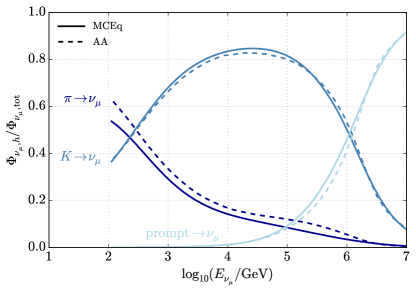
Figure 1: Fraction of muons (left) and muon neutrinos (right) from pions, kaons and prompt sources integrated over zenith angle.

The decay moments follow from the two-body decay kinematics of charged pions and kaons. In particular,

$$Z_{\pi\mu}(\gamma)\,=\,\frac{(1-r_{\pi}^{\gamma+1})}{(\gamma+1)(1-r_{\pi})}\,=\,\int_{r_{\pi}}^{1}x^{\gamma}\frac{{\rm d}n_{\mu}}{{\rm d}x}{\rm d}x$$ (7)

and

$$Z_{\pi\mu}(\gamma+1)\,=\,\frac{(1-r_{\pi}^{\gamma+2})}{(\gamma+2)(1-r_{\pi})},$$ (8)

where $x=E_{\mu}/E_{\pi}$, $\gamma$ is the integral spectral index of the cosmic-ray spectrum and $r_{\pi}=(m_{\mu}/m_{\pi})^{2}\approx 0.573$. The forms for two-body decay of charged kaons are the same but with $r_{K}=(m_{\mu}/m_{K})^{2}\approx 0.046$. The corresponding forms for decay to muon neutrinos are

$$Z_{M\nu}(\gamma)=\frac{(1-r_{M})^{\gamma+1}}{(\gamma+1)(1-r_{M})}$$ (9)

and

$$Z_{M\nu}(\gamma+1)\,=\,\frac{(1-r_{M})^{\gamma+2}}{(\gamma+2)(1-r_{M})}.$$ (10)

Because $r_{\pi}$ is large, the muon carries most of the energy in pion decay, while in kaon decay the energy is shared almost equally between the muon and the neutrino. As a consequence, the kaon channel becomes the dominant source of $\nu_{\mu}$ above $\sim 100$ GeV where Eq. (10) applies. These effects are illustrated in Fig. 1.

A standard approximation is to combine the low Eq. (2) and high Eq. (3) energy forms into a single equation of the form [1]

$$\frac{{\rm d}N_{\ell}}{{\rm d}E_{\ell}}=\frac{N_{0}(E_{\ell})}{1-Z_{NN}}\left\{\frac{A_{\pi\ell}}{1+B_{\pi\ell}\cos\theta\,E_{\ell}/\epsilon_{\pi}}+\frac{A_{K\ell}}{1+B_{K\ell}\cos\theta\,E_{\ell}/\epsilon_{K}}\right\}.$$ (11)

This formula applies to $\mu^{+}+\mu^{-}$ and to $\nu_{\mu}+\bar{\nu}_{\mu}$. For the treatment of separate charges we refer to Ref. [4]. Prompt leptons can be treated by adding a term of the same form as for pions and kaons to Eq. (11) and using the appropriate decay distributions. Typically, however, the analytic approximations contain a limited number of cascade channels. For example, Eq. (11) neglects production of kaons by pions (and vice versa). In addition, since resonance production is not included, the input data fot the spectrum-weighted moments most include pions and kaons from decay of resonances.

Equation 11 can be generalized to include the slow energy-dependence of cross sections as well as a smooth bending of the primary spectrum by evaluating spectrum weighted moments following the prescription of Thunman, Ingelman and Gondolo [3]:

$$Z_{NM}(E)=\int_{E}^{\infty}\frac{N_{0}(E^{\prime})}{N_{0}(E)}\frac{\sigma(E^{\prime})}{\sigma(E)}\frac{{\rm d}n_{NM}(E^{\prime},E)}{{\rm d}E}{\rm d}E^{\prime}\rightarrow\int_{0}^{1}\,x^{\gamma}\frac{{\rm d}n_{NM}(x)}{{\rm d}x}\,{\rm d}x.$$ (12)

For a power-law primary spectrum with integral spectral index $\gamma$ and constant cross sections the definition collapses to the standard scaling definition in terms of $x=E/E^{\prime}$. The energy dependence of the decay factors is accounted for by using an energy-dependent spectral index, $\gamma(E)$. Note that here also, the generalized spectrum weighted moments are evaluated at the energy of the lepton.

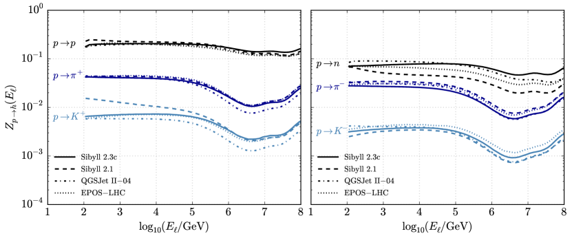
Figure 2: Energy-dependent Z-factors calculated with various hadronic models for the H3a nucleon spectrum [4]. Left: positive secondaries; Right: neutrons and negative mesons.

The next section discusses atmospheric leptons from $100$ GeV to $>10$ PeV. For such high-energy leptons $\gg 100$TeV it is necessary to use the energy-dependent version of the Z-factors defined in Eq. (12) to take account of the knee in the primary spectrum in the PeV range. Fig. 2 compares the Z-factors for the four interaction models used for comparison in this paper (Sibyll-2.3c [5], Sibyll-2.1 [6], EPOS-LHC [7] and QGSJetII-04 [8]).

The Matrix Cascade Equation (MCEq) program [9, 10] solves Eq. (1) by starting with a nucleon of energy $E_{0}$ and integrating by matrix multiplication at each step of ${\rm d}X$, using one of the standard hadronic interaction models to calculate production of particles. It follows 65 particle types with an energy grid of eight bins per decade of energy, and it includes energy loss for charged particles. Thus the two main limitations of the approximate formulas (limited channels and the interpolation between low and high energy) are absent. On the other hand, the analytic approximations are parameterised directly in terms of the underlying physical processes. In this paper we compare several results of the analytic approximations (hereafter AA) with those of MCEq. The goal, using MCEq as the standard, is to compare errors and limitations of the approximate formulas with differences between the different cosmic-ray event generators.

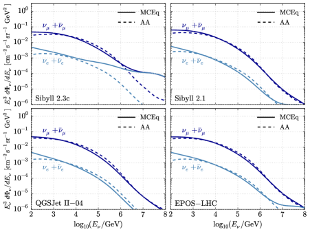
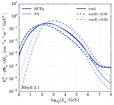
Figure 3: Left: Comparison of neutrino fluxes averaged over zenith angle for four hadronic interaction models (solid, MCEq; dashed AA) with the H3a spectrum of Ref. [4]. Right: The calculation with Sibyll-2.1 for muons, also shown for $\cos\theta=0.95$ and $\cos\theta=0.05$ separately.

2 Comparison of lepton fluxes

In this section we show examples of fluxes of muons and neutrinos. In Fig. 3 the comparisons between MCEq and AA for neutrinos are shown for Sibyll-2.3c [5], Sibyll-2.1 [6], EPOS-LHC [7] and QGSJetII-04 [8]. The AA calculations do not include prompt neutrinos, which are present in Sibyll-2.3c, but not in the other models. In addition, AA does not include neutrinos from decay of muons, which are significant below a TeV, especially for $\nu_{e}$. The right panel of the figure compares MCEq and AA averaged over zenith angle for Sibyll-2.1, which does not include charm. However, it does include prompt muons from the $\mu^{+}+\mu^{-}$ branch of neutral vector mesons decay, which accounts for the rise in the MCEq muon flux at high energy. The AA muon calculation accounts for muon energy loss with an approximation due to Lipari [11] and described in Ref. [1]. The excess of MCEq in electron neutrinos towards low energies is the contribution from decays of secondary muons, a process that is currently missing in the AA.

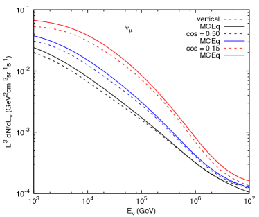
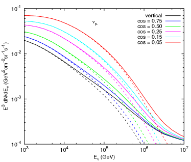
Figure 4: Left: Comparison of muon neutrino fluxes $\nu_{\mu}+\bar{\nu}_{\mu}$ using Sibyll-2.3c and the H3a flux (solid, MCEq; dashed AA); Right: Flux of $\nu_{\mu}+\bar{\nu}_{\mu}$ for several zenith angles (AA conventional neutrinos with broken lines).

Fig. 4 illustrates the fact that the flux of high-energy atmospheric neutrinos increases significantly toward the horizon as a consequence of the ”secant$\theta$” effect from the $1/\cos\theta$ factor in Eq. (11). The prompt contribution to neutrino event rates is much smaller than the impression given by the amplification by $E^{3}$ in the plot. The flux of atmospheric neutrinos increases by almost an order of magnitude from vertical to horizontal in the 10 to 100 TeV energy range, in contrast to the isotropic expectation for a diffuse astrophysical flux.

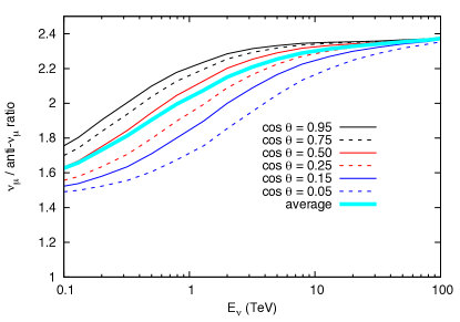
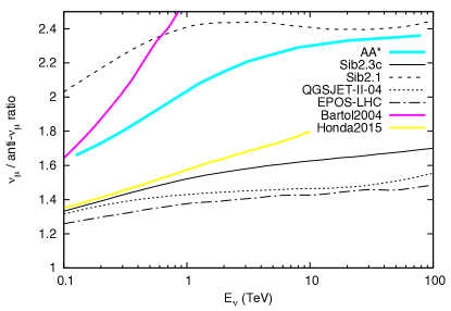
Figure 5: Left: The predicted ratio $\nu_{\mu}/\bar{\nu}_{\mu}$ for a range of $\cos\theta$ ; Right: Ratios averaged over zenith angle from six specific interaction models compared to the analytical approximation using OPERA parameters (AA*), as described in the text.

3 Charge ratio

The increasing importance of the kaon channel at high energy (Fig. 1) leads to an increase in the muon charge ratio at TeV energies. This is a consequence of the fact that the charge ratio of kaons is larger than that of pions. The muon charge ratio also depends on the parameter $\delta_{0}=(p-n)/(p+n)$, the proton excess in the spectrum of primary nucleons. The OPERA Experiment [12] fit their measurement of the muon charge ratio using the parameterisation of Ref. [4] with the two main parameters, $\delta_{0}$ and $Z_{pK^{+}}$, adjusted to fit their data. Here we show in the left panel of Fig. 5 the predicted $\nu_{\mu}/\bar{\nu}_{\mu}$ ratio calculated using the OPERA parameters (AA*). The right panel compares MCEq calculations of the $\nu_{\mu}/\bar{\nu}_{\mu}$ ratio for the four event generators for air showers as well as two Monte Carlo calculations at low energy, Bartol2004 [13] and Honda2015 [14]. The left plot illustrates how the ratio evolves with energy as a function of zenith angle, which follows from the $E_{\nu}\cos\theta$ dependence in Eq. (11).

4 Seasonal variation of muons

A traditional measurement for any underground cosmic-ray detector is the seasonal variation of the muon rate. The range of depths of various detectors corresponds to an energy range from below ($100$ GeV) to several TeV [15]. The temperature dependence enters through the pion and kaon critical energies, which are proportional to the absolute temperature as a function of atmospheric depth from Eq. (4). The full analysis for the IceCube detector at the South Pole is described in Ref. [2] presented at this conference. The extreme temperatures at the South Pole make this an interesting test of the comparison between AA and MCEq, as illustrated in Fig. 6.

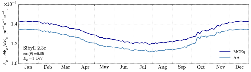
Figure 6: Atmospheric muon rate at $E_{\mu}=1\,\mathrm{TeV}$ and $\cos\theta=0.85$ from MCEq and AA calculations for each day of the year 2012 using Sibyll-2.3c and the H3a cosmic ray flux.

The full calculation for the South Pole [2] requires accounting for the energy-dependence of the acceptance for muons in IceCube as well as the energy dependence of muon production. Here we show the calculated muon rate for $E_{\mu}=1$ TeV for each day in 2012, which is independent of IceCube response to muons. Using the same temperature data for the South Pole from the AIRS Satellite [16], both the overall seasonal variation as well as short term features are reproduced well. The AA normalization is about 5% lower than that of MCEq, and the short-term features are sharper in AA.

5 Conclusion

Lepton fluxes calculated with the analytic approximations generally agree within 5-20% depending on energy and angle (e.g. Figs. 4 and 6). Differences among the post-LHC models are in some cases larger as can be seen from Fig. 2. The largest difference is between Sibyll-2.3c and QGSJetII-04 for which $K^{+}$ differ by $\approx 40$% while $K^{-}$ are almost the same. The situation is similar for pions in that $\pi^{-}$ are comparable in the two models and $\pi^{+}$ are $\approx 15$% higher in Sibyll-2.3c. EPOS-LHC is intermediate. The charge ratio differences are also reflected in the differences among the models for the $\bar{\nu}_{\mu}/\nu_{\mu}$ in the right panel of Fig. 5. Interestingly, the prediction for the $\bar{\nu}_{\mu}/\nu_{\mu}$ ratio based on parameters of the muon charge ratio measurement from OPERA [12] is higher than all the post-LHC models.

References

- [1] T. K. Gaisser, R. Engel and E. Resconi, “Cosmic Rays and Particle Physics : 2nd Edition,” (Cambridge University Press, 2016).
- [2] IceCube Collaboration, S.Tilav et al., “Seasonal variation of atmospheric muons in IceCube,” \posPoS(ICRC2019)894 (these proceedings).
- [3] P. Gondolo, G. Ingelman and M. Thunman, “Charm production and high-energy atmospheric muon and neutrino fluxes,” Astropart. Phys. 5, 309 (1996) [arXiv:9505417 [hep-ph]].
- [4] T. K. Gaisser, “Spectrum of cosmic-ray nucleons, kaon production, and the atmospheric muon charge ratio,” Astropart. Phys. 35, 801 (2012) [arXiv:1111.6675 [astro-ph.HE]].
- [5] F. Riehn, H. P. Dembinski, R. Engel, A. Fedynitch, T. K. Gaisser and T. Stanev, “The hadronic interaction model SIBYLL 2.3c and Feynman scaling,” \posPoS(ICRC2017)301 (2018).
- [6] E. J. Ahn, R. Engel, T. K. Gaisser, P. Lipari and T. Stanev, “Cosmic ray interaction event generator SIBYLL 2.1,” Phys. Rev. D 80, 094003 (2009) [arXiv:0906.4113 [hep-ph]].
- [7] T. Pierog, I. Karpenko, J. M. Katzy, E. Yatsenko and K. Werner, “EPOS LHC: Test of collective hadronization with data measured at the CERN Large Hadron Collider,” Phys. Rev. C 92, no. 3, 034906 (2015) [arXiv:1306.0121 [hep-ph]].
- [8] S. Ostapchenko, “QGSJET-II: physics, recent improvements, and results for air showers,” EPJ Web Conf. 52, 02001 (2013).
- [9] A. Fedynitch, R. Engel, T. K. Gaisser, F. Riehn and T. Stanev, “Calculation of conventional and prompt lepton fluxes at very high energy,” EPJ Web Conf. 99, 08001 (2015) [arXiv:1503.00544 [hep-ph]].
- [10] A. Fedynitch, H. Dembinski, R. Engel, T. K. Gaisser, F. Riehn and T. Stanev, “A state-of-the-art calculation of atmospheric lepton fluxes,” \posPoS(ICRC2017)1019 (2018).
- [11] P. Lipari, “Lepton spectra in the Earth’s atmosphere,” Astropart. Phys. 1, 195 (1993).
- [12] OPERA Collaboration, N. Agafonova et al., “Measurement of the TeV atmospheric muon charge ratio with the complete OPERA data set,” Eur. Phys. J. C 74, 2933 (2014) [arXiv:1403.0244 [hep-ex]].
- [13] G. D. Barr, T. K. Gaisser, P. Lipari, S. Robbins and T. Stanev, “A Three - dimensional calculation of atmospheric neutrinos,” Phys. Rev. D 70, 023006 (2004) [arXiv:0403630 [astro-ph]].
- [14] M. Honda, M. Sajjad Athar, T. Kajita, K. Kasahara and S. Midorikawa, “Atmospheric neutrino flux calculation using the NRLMSISE-00 atmospheric model,” Phys. Rev. D 92, no. 2, 023004 (2015) [arXiv:1502.03916 [astro-ph.HE]].
- [15] MINOS Collaboration, P. Adamson et al., “Observation of Seasonal Variation of Atmospheric Multiple-Muon Events in the MINOS Near and Far Detectors,” Phys. Rev. D 91, no. 11, 112006 (2015) [arXiv:1503.09104 [hep-ex]].
- [16] https://airs.jpl.nasa.gov/data/overview