Anomalies in the switching dynamics of C-type antiferromagnets and antiferromagnetic nanowires

Abstract

Antiferromagnets (AFMs) are widely believed to be superior than ferromagnets in spintronics because of their high stability due to the vanishingly small stray field. It is thus expected that the order parameter of AFM should always align along the easy-axis of the crystalline anisotropy. In contrast to this conventional wisdom, we find that the AFM order parameter switches away from the easy-axis below a critical anisotropy strength when an AFM is properly tailored into a nano-structure. The switching time first decreases and then increases with the damping. Above the critical anisotropy, the AFM order parameter is stable and precesses under a microwave excitation. However, the absorption peak is not at resonance frequency even for magnetic damping as low as 0.01. To resolve these anomalies, we first ascertain the hidden role of dipolar interaction that reconstructs the energy landscape of the nano-system and propose a model of damped non-linear pendulum to explain the switching behavior. In this framework, the second anomaly appears when an AFM is close to the boundary between underdamped and overdamped phases, where the observed absorption lineshape has small quality factor and thus is not reliable any longer. Our results should be significant to extract the magnetic parameters through resonance techniques.

I Introduction

Ferromagnets played a vital role in the early development of magnetism, as well as the modern spintronics since late 1980s, while studies and applications of antiferromagnets (AFMs) are quite limited for their lack of tunability, thus useless. In the last few years, AFMs started to attract significant attention after the discovery of electrical knob to control antiferromagnetic order in a class of antiferromagnets with broken inversion symmetry Wadley2016 ; Zelezny2014 . Various aspects, such as damping mechanism Yuan20172 ; Yuan20171 , spin transfer torque Kimel2004 ; Duine2007 ; Haney2008 ; Xu2008 , magnetic switching Wadley2016 , spin pumping Cheng2014 , domain wall/skyrmion dynamics Gomonay2010 ; Hals2011 ; Helen2016 ; Shiino2016 ; Selzer2016 ; Jungwirth2016 ; Xichao2016 ; Barker2016 ; Yuan2018a ; Yuan2018b have been extensively investigated. One strong motivation of such intense interest in AFMs is their abundance in nature and intriguing stability due to the vanishingly small magnetostatic interaction (MI), which is ever doomed to be its drawback. Accordingly, MI is neglected in most of the theoretical and numerical studies of AFMs Hals2011 ; Shiino2016 ; Selzer2016 ; Helen2016 . Nevertheless, the magnetic dipoles are there and the distribution of the dipoles in an AFM will potentially influence the magnetic energy and thus the magnetization dynamics, similar to the situation of electric dipoles in dielectric materials such as liquid crystals stephen1974 . One open question is when and how the MIs manifest themselves and influence the magnetization dynamics. A complete understanding of this issue may help us in designing AFM-based devices that are truly free from the perturbation of magnetic charges.

In this work, we take the first step to show that MI can induce a switching of an AFM order when its crystalline anisotropy is below a critical value. The switching occurs at an ultrafast scale and widely exists in C-type AFMs and AFM nanowires. By analytically calculating the interaction of magnetic charges, we find that MI produces an effective anisotropy that is quadratic in magnetic order and thus reconstructs the energy landscape of the system, which have observable effect on magnetization switching and spin wave spectrum. Above the critical anisotropy, AFM resonance is observed, but the absorption peak does not position at the true resonance frequency when the magnetic damping is close to a critical value around 0.01. A detailed analysis shows that the quality factor of the absorption lineshape is significantly reduced by the critical damping, near which the system enters the overdamped regime and the Kittel theory based on the Lorentz lineshape fails.

This article is organized as follows. Our model, methodologies, and main findings are presented in Sec. II. In Sec. III, we explain the anomalous resonance behavior near the phase boundaries and list the typical order of critical damping for the commonly used AFMs. Discussions and conclusions are given in Sec. IV, followed by acknowledgments.

II Model and results

We first consider a two-sublattice antiferromagnetic nanowire with an easy-axis along the longitudinal direction as shown in Fig. 1(a). The magnetization dynamics is first studied by numerically solving the Landau-Lifshitz-Gilbert (LLG) equation Vansteenkiste2014 ,

$$\frac{\partial\mathbf{S}_{i}}{\partial t}=-\gamma\mathbf{S}_{i}\times\mathbf{H}_{i}+\frac{\alpha}{S}\mathbf{S}_{i}\times\frac{\partial\mathbf{S}_{i}}{\partial t},$$ (1)

where $\mathbf{S}_{i}$ is the dimensionless spin vector at $i-$th site with magnitude $S$, $\gamma$ is gyromagnetic ratio, and $\alpha$ is Gilbert damping. $\mathbf{H}_{i}$ is the effective field acting on $\mathbf{S}_{i}$, including antiferromagnetic exchange field between two nearest spins, crystalline anisotropy field and stray field. The effective field can be quantitatively evaluated as $\mathbf{H}_{i}=-\delta\mathcal{H}/\delta\mathbf{S}_{i}$. The Hamiltonian $\mathcal{H}$ reads,

$$\mathcal{H}= J\sum_{\langle i,j\rangle}\mathbf{S}_{i}\cdot\mathbf{S}_{j}-K\sum_{i}\mathbf{S}_{i,x}^{2}-\frac{\mu_{0}\mu_{s}}{2S}\sum_{i}\mathbf{S}_{i}\cdot\mathbf{H}_{d,i},$$ (2)

where the first, second and third terms represent the exchange, crystalline anisotropy and magnetostatic energy, respectively. $J,K,\mu_{0},\mu_{s}$ are respectively exchange coefficient, crystalline anisotropy coefficient, vacuum permeability and the magnitude of local magnetic moments. $\mathbf{H}_{d,i}$ is dipolar field acting on the spin $\mathbf{S}_{i}$. The factor 1/2 is introduced to eliminate the duplicate calculation of magnetostatic energy.

To simulate the dynamics of the system, the parameters are taken to mimic commonly used AFM $\mathrm{Mn_{2}Au}$ with $J=24$ meV Sapozhnik2018 , and $\mu_{s}=3.59\mu_{B}$, where $\mu_{B}$ is Bohr magneton. Note that the anisotropy of $\mathrm{Mn_{2}Au}$ is sensitive to the magnitude of strain Shick2010 and the magnitude of damping ($\alpha$) is still lacking of experimental characterization, thus we treat them as free parameters. Our main findings are: (1) The antiferromagnetic order switches spontaneously away from the easy-axis ($x-$axis) toward the transverse direction for crystalline anisotropy $K<1.55~{}\mu\mathrm{eV}$ (15 mT). Two typical switching events are shown in the inset of Fig. 1(b). For $\alpha<\alpha_{c}\sim 0.01$, the switching is accompanied by ultrafast oscillation of magnetization while the switching is monotonic for larger dampings. (2) The switching time first decreases and then increases with the damping and the minimum locates around the critical damping, which separates the oscillation phase from the monotonic phase. As a comparison, no switching happens for the ferromagnetic counterpart with exactly the same parameters except the sign of exchange coefficient ($J$). Next we will show that this anomalous switching of an AFM resulting from the effect of MI and the oscillation/monotonic phase can be understood from the underdamped and overdamped phenomena of a pendulum-like motion of AFM order parameter.

II.1 Theoretical formalism

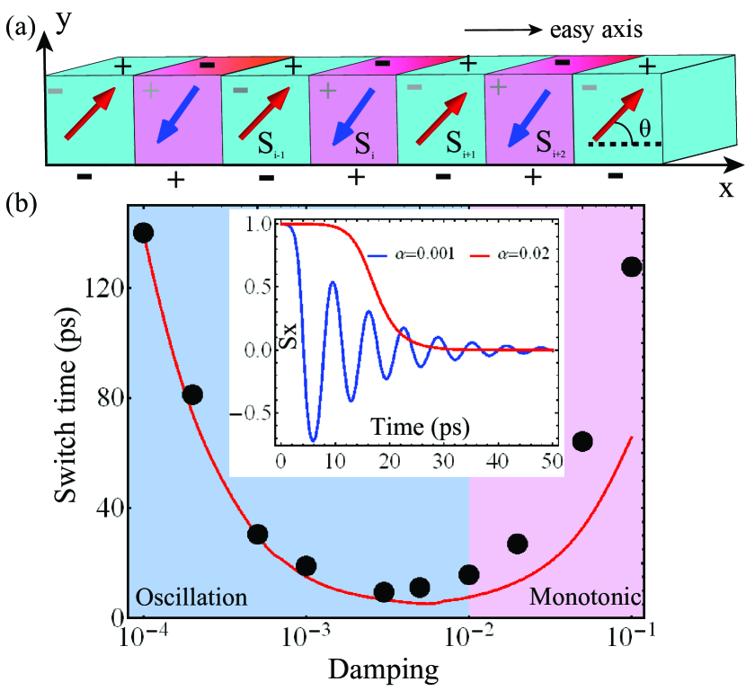
Figure 1: (a) Schematic illustration of a two-sublattice antiferromagnetic nanowire. The red and blue arrows respectively represent the magnetic moments on each sublattice. The easy-axis of crystalline anisotropy is along the $x-$axis. The $\pm$ signs indicate the distribution of magnetic charges on the surface (black) and inside the volume (gray). (b) Switching time of magnetic order as a function of damping. The red line is theoretical prediction of Eq. (6). The light-blue and light-pink region represent the oscillating and monotonic phases, respectively. The inset shows the two typical switching modes in the two phases for $\alpha=0.001$ (blue line) and $\alpha=0.02$ (red line), respectively.

To understand the anomalous switching behavior, the key point is to properly consider the demagnetization effect in this system. Here both the volume and surface charges contribute to the magnetostatic field $\mathbf{H}_{d}$, and it can be formally evaluated as,

$$\mathbf{H}_{d,i}=-M_{s}/S\sum_{j}\mathbf{N}_{ij}\cdot\mathbf{S}_{j},$$ (3)

where $M_{s}=\mu_{s}/a^{3}$ is the saturation magnetization, with $a$ being the distance of two neighboring spins, $\mathbf{N}_{ij}$ is the demagnetization tensor that depends only on the distance of two spins Newell1993 .

Suppose the system is in a Néel state with $\mathbf{S}_{i}=(-1)^{i}S(\cos\theta\mathbf{e}_{x}+\sin\theta\mathbf{e}_{y})$, as shown in Fig. 1(a) and the longitudinal dimension $N\gg 1$, then the total energy of the system can be calculated as,

$$E(\theta) =-(N-1)JS^{2}-NKS^{2}\cos^{2}\theta$$ (4)

$$+Na^{3}K_{d}(D_{\parallel}\cos^{2}\theta+D_{\perp}\sin^{2}\theta),$$

where $K_{d}=\mu_{0}M_{s}^{2}/2$, $D_{\parallel}=N^{xx}_{r=0}+2\sum_{p=1}^{N/2}(-1)^{p}N^{xx}_{r=pa},D_{\perp}=N^{yy}_{r=0}+2\sum_{p=1}^{N/2}(-1)^{p}N^{yy}_{r=pa}$, $r=|i-j|a$ is the distance between two spins. The factor $(-1)^{p}$ comes from the antiparallel (parallel) alignment of two spins separating with odd (even) number of $a$, which disappears for a ferromagnetic state. Since the magnetostatic energy of two spins decays with their distance as $1/r^{3}$ jackson , two well-separated spins with large separation do not contribute to the energy significantly. Here we use a cut-off distance of $r=4a$, and analytically derive $D_{\parallel}=0.5713,D_{\perp}=0.2144$ by evaluating the demagnetization tensors ($N^{xx}_{r}$ and $N^{yy}_{r}$) directly. A choice of a larger cut-off distance will not change $D_{\parallel}$ or $D_{\perp}$ more than $1\%$.

Here we pay special attention to the longitudinal magnetization states (LS, $\theta=0$) and transverse states (TS, $\theta=\pi/2$). The energy difference of these two states can be explicitly calculated as, $\Delta E/N=-KS^{2}+K_{d}(D_{\parallel}-D_{\perp})$. For an AFM with strong crystalline anisotropy, the LS is energy preferable while the TS becomes energy preferable when the anisotropy is very weak. The critical anisotropy can be evaluated from $\Delta E=0$ as $K_{c}=K_{d}(D_{\parallel}-D_{\perp})$. Figure 2(a) shows the energy landscape of the system as a function of spin orientation $\theta$ for $K=0$ (black line), $K_{c}$ (red line) and $2K_{c}$ (blue line), respectively. Clearly, LS (TS) has lower energy than TS (LS) for $K>K_{c}$ ($K<K_{c}$). Then it is expected that the antiferromagnet will spontaneously switch from LS to TS for $K<K_{c}$, where the crystalline anisotropy can be reduced by electrical means Weisheit2007 ; Maruyama2009 ; Lebeugle2009 .

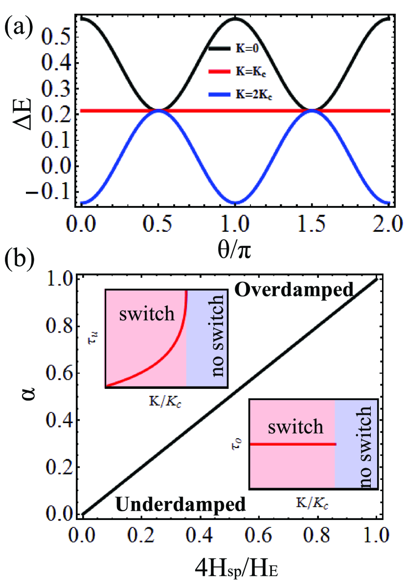
Figure 2: The energy landscape of the system as a function of spin orientation $\theta$ for $K=0$ (black line), $K_{c}$ (red line), $2K_{c}$ (blue line), respectively. The vertical axis is scaled by $NK_{d}$. (b) Phase diagram of the system in $4H_{\mathrm{sp}}/H_{E}\sim\alpha$ plane. The top-left and bottom-right insets show the typical switching time as a function of crystalline anisotropy for overdamped regime and underdamped regime, respectively.

To analytically describe this switching process, we recall the antiferromagnetic dynamic equations in terms of the staggered order Yuan2018a ,

$$\mathbf{n}\times(\partial_{tt}\mathbf{n}+\alpha H_{E}\partial_{t}\mathbf{n}-H_{E}\mathbf{h}_{n})=0\ ,$$ (5)

where $\mathbf{n}\equiv(\mathbf{S}_{2i}-\mathbf{S}_{2i+1})/2S$ is the staggered order, $H_{E}\equiv 8JS$ is homogeneous exchange field, $\mathbf{h}_{n}=4(K-K_{c})\mathbf{e}_{x}$ is the effective anisotropy field acting on the staggered order. In spherical coordinates, the dynamic equations can be recast as,

$$\frac{\partial^{2}\psi}{\partial t^{2}}+2\zeta\omega_{0}\frac{\partial\psi}{\partial t}+\mathrm{sgn}(K-K_{c})\omega_{0}^{2}\sin\psi=0,$$ (6)

where $\psi=2\theta,\zeta=\alpha H_{E}/(4H_{\mathrm{sp}}),\omega_{0}=\gamma H_{\mathrm{sp}}$, $H_{\mathrm{sp}}=\sqrt{H_{\mathrm{E}}K_{\mathrm{eff}}}$ is the spin-flop field, $K_{\mathrm{eff}}=|K-K_{c}|$ is the effective anisotropy coefficient that has included the contribution from MI. The sign function $\mathrm{sgn}(x)=1$ for $x\geq 0$ and $-1$ for $x<0$. This equation is similar to the dynamics of a damped non-linear pendulum Kim2014 . In general, the solution to Eq. (6) is an elliptic function with a complicated time dependence Kim2014 . To have some insights on the time scale of the system, we shall solve Eq. (6) under small amplitude approximation ($\sin\psi\sim\psi$).

According to the value of damping ratio $\zeta$, three regimes can be classified. (i) Underdamped regime ($\zeta<1$, i.e. $\alpha<4H_{\mathrm{sp}}/H_{E}$): The solution $\psi(t)=\psi_{0}e^{-\zeta\omega_{0}t}\sin(\sqrt{1-\zeta^{2}}\omega_{0}t+\varphi_{0})$. The system oscillates and decays to the equilibrium state with a time-scale of $\Delta t=1/(\zeta\omega_{0})$, i.e. the larger the damping is, the faster the relaxation will be. This is consistent with the oscillation phase in Fig. 2(b). (ii) Overdamped regime ($\zeta>1$, i.e. $\alpha>4H_{\mathrm{sp}}/H_{E}$): $\psi(t)=\psi_{0}e^{-\zeta\omega_{0}t}(c_{1}e^{\sqrt{\zeta^{2}-1}\omega_{0}t}+c_{2}e^{-\sqrt{\zeta^{2}-1}\omega_{0}t})$. Two modes $1/\tau_{s}=(\zeta-\sqrt{\zeta^{2}-1})\omega_{0}$ and $1/\tau_{f}=(\zeta+\sqrt{\zeta^{2}-1})\omega_{0}$ compete to determine the dynamics, while the long-time behavior of the pendulum is dominated by the slow mode $\tau_{s}$. Since $\tau_{s}$ increases with the damping ratio, the relaxation time becomes larger with the increase of damping. This is also consistent with the monotonic phase in Fig. 2(b). (iii) Critical regime ($\zeta=1$, i.e. $\alpha=4H_{\mathrm{sp}}/H_{E}$): $\psi(t)=\psi_{0}e^{-\zeta\omega_{0}t}$. A complete phase diagram in the $4H_{\mathrm{sp}}/H_{E}\sim\alpha$ plane is shown in Fig. 2(b). The typical overdamped and underdamped cases are shown in the top-left and bottom-right panels, respectively. They show distinguished anisotropy dependences.

As a comparison, the ferromagnetic counterpart of Eq. (6) reads yin2018 ,

$$\frac{\partial\theta}{\partial t}=-\alpha\gamma K_{\mathrm{eff}}\sin 2\theta$$ (7)

which is a first-order ordinary differential equation. This equation can be analytically solved as $-(t-t_{0})/\Delta t=\ln\tan\theta$, where $\Delta t=1/(2\alpha\gamma K_{\mathrm{eff}})$. Differing from antiferromagnets, the typical switching time does not depend on the strong exchange constant $H_{E}$ and it usually takes a longer time to reach the steady state because of $K_{\mathrm{eff}}\ll H_{E}$.

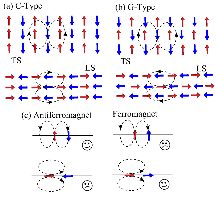
Figure 3: Schematic illustration of an antiferromagnet with C-type ordering (a) and G-type ordering (b) in 2D, respectively. The dashed lines indicate the flow of magnetostatic fields generated by the central spin. (c) Schematic illustration of the difference between two antiferromagnetically and ferromagnetically coupled spins. The smile and disappointed faces refer to low energy and high energy states, respectively.

II.2 2D/3D cases

Up till now, we focused on the switching behavior of a 1D magnetic nanowire, but the essential physics is still valid for C-type antiferromagnet in 2D and 3D cases. To be specific, as shown in Fig. 3(a), the magnetostatic field of a particular spin (dashed line) always align parallel(antiparallel) with the nearest spins for TS (LS) state in C-type antiferromagnet. Hence, the TS state is energetically favorable. For G-type antiferromagnet or checkerboard antiferromagnet, LS and TS is energetically degenerated, which can be seen in Fig. 3(b). For reference, Table 1 lists the strength of anisotropy coefficients induced by MI in various spin ordering of antiferromagnets, which is calculated using the technique presented in Sec. IIA. As the spatial dimension increases from 1D to 3D, the influence of the MI ($D_{\parallel}/D_{\perp}$) becomes more significant for C-type antiferromagnets.

Item	1D	2D-CT	2D-GT	3D-CT	3D-GT
$D_{\parallel}$	0.5713	0.7369	0.4163	0.9922	0.3350
$D_{\perp}$	0.2144	0.0022	0.4163	0.0028	0.3350

Table 1: List of the effective anisotropy coefficients generated by magnetostatic interaction in various spin orderings. 2D square lattice and 3D simple cubic lattice are used to calculated these values. The symbols CT and GT are short for C-type and G-type ordering, respectively.

Before going on, we emphasize that the effective anisotropy caused by MI is very different from ferromagnetic counterpart known as the shape anisotropy. Use a 1D nanowire of sufficiently long length as an example, the demagnetization factor is $D_{\parallel}=0,D_{\perp}=0.5$ for a ferromagnet fmdemag , which implies that the magnetization always tends to align in the longitudinal direction. For an antiferromagnet, the transverse direction is preferred by MI. This difference motivates this work that the distribution of magnetic dipoles on atomic scale will inevitably lead to a very different energy landscape of the system. A schematic illustration of this difference in a simple two-dipole model is given in Fig. 3(c), the physics is as follows. Along a line, the head-to-tail (ferromagnetic state) is the lowest energy state and head-to-head (anti-ferromangetic configuration) is the highest one. On the other hand, for two dipoles in shoulder-to-shoulder, the lower energy configuration is the antiferromagnetic arrangement, and the ferromagnetic one is the highest one.

II.3 Spin wave spectrum modification

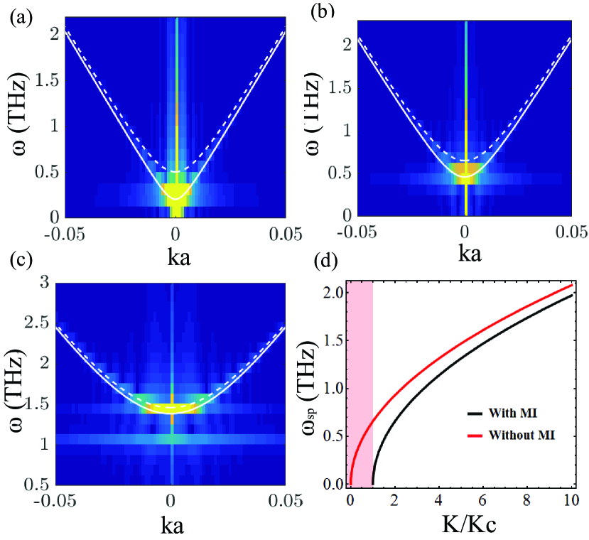
Figure 4: Spin-wave spectrum of an antiferromagnetic nanowire after fully taking account of the magnetostatic interaction. The color codes the Fourier transform amplitude of $S_{y}(x,t)$. The white solid-line is the theoretical prediction with MI while the white dashed-line is the prediction without MI. (a) $K=1.2K_{c}$, (b) $K=2K_{c}$, (c) $K=10K_{c}$. (d) The magnetic resonance frequency as a function of crystalline anisotropy with (black line) and without MI (red line). The light red region indicates the regime that spontaneous switching occurs. $H=0$, $h_{0}=0.2$ T, $\omega=10$ THz, $\alpha=10^{-4}$.

Theoretically, the spin-wave dispersion near an antiferromagnetic Néel state is weiwei2017 ; yuan2017apl ,

$$\omega=\pm\gamma H+\gamma\sqrt{H_{\mathrm{sp}}^{2}+4J^{2}\sin^{2}ka},$$ (8)

where $H$ is external field, $k$ is spin wave vector. For $k=0,H=0$, we recover the magnetic resonance frequency $\omega_{0}=\gamma\sqrt{H_{\mathrm{E}}K_{\mathrm{eff}}}=2\gamma\sqrt{2JK_{\mathrm{eff}}}$. Since $K_{\mathrm{eff}}<K$ for $K>K_{c}$, the spin-flop field will become smaller under the influence of MI and the spin-wave frequency tends to have a red shift.

To verify these predictions, we add a magnetic field pulse $\mathbf{h}(t)=h_{0}\mathrm{sinc}(\omega t)\mathbf{e}_{y}$ to excite spin-waves in an antiferromagnetic nanowire and calculate the time dependence of $\mathbf{S}(x,t)$ by numerically solving the LLG equation. By taking a 2D Fourier transform of $S_{y}(x,t)$, we obtain the spin-wave spectrum in $(k,\omega)$ plane as shown in Fig. 4(a) ($K=1.2K_{c}$), 4(b) ($K=2K_{c}$) and 4(c) ($K=10K_{c}$). Clearly, the dispersion can only be reproduced by including the influence of MI (white solid-line), especially the magnetic resonance mode located at $k=0$. As $k$ increases, the influence of anisotropy becomes small as indicated by the merging trend of the solid and dashed lines. We also plot the comparison of resonance frequency as a function of crystalline anisotropy in Fig. 4(d). The role of magnetostatic interaction becomes most significant when $K/K_{c}\rightarrow 1$.

III Antiferromagnetic resonance

Magnetic resonance represents large amplitude oscillation of magnetic order when the driving frequency matches the natural frequency of the magnet. In experiments, by measuring the position of maximum absorption and the linewidth of resonant spectrum, one can extract the magnetic parameters such as anisotropy and magnetic damping. In this section, we show that this common understanding has some intrinsic problems for an antiferromagnet when the damping is close to a critical value, which is on the order of the ratio of spin-flop field and the exchange field ($\sim 0.01$ for $K_{\mathrm{eff}}\sim 10^{-4}H_{\mathrm{E}}$).

Let us start from the dynamic equations in terms of the two-sublattice magnetic moments Eq. (1). Here we consider the regime $K>K_{c}$, By setting $\partial\mathbf{S}_{i}/\partial t=0$, we find the ground state of the system is a Néel state along $x-$axis, as shown in Fig. 1(a) with $\theta=0$. Generally, the magnetic moments will perform uniform oscillations near this ground state under the action of an oscillating field $\mathbf{h}=\mathbf{h}e^{-i\omega t}$, i.e. $\mathbf{S}_{2i}=S\mathbf{e}_{x}+\delta\mathbf{S}_{a}(t),\mathbf{S}_{2i+1}=-S\mathbf{e}_{x}+\delta\mathbf{S}_{b}(t)$. By substituting the trial solutions into Eq. (1) and keeping only the terms linear in $\delta\mathbf{S}_{a,b}$, we obtain

$$i\frac{\partial}{\partial t}\left(\begin{array}[]{c}\delta S_{a}^{+}\\ \delta S_{b}^{+}\end{array}\right)=\mathbf{DH}_{0}\left(\begin{array}[]{c}\delta S_{a}^{+}\\ \delta S_{b}^{+}\end{array}\right)+\mathbf{D}\left(\begin{array}[]{c}-h_{+}\\ h_{+}\end{array}\right),$$ (9)

where $\delta S_{a}^{+}=\delta S_{a}^{y}+i\delta S_{a}^{z},h_{+}=h_{y}+ih_{z}$. $\mathbf{D}=\mathrm{diag}((1-i\alpha)^{-1},(1+i\alpha)^{-1})$ is dissipation matrix, $\mathbf{H}_{0}$ is the effective Hamiltonian in the absence of damping,

$$\mathbf{H}_{0}=\left(\begin{array}[]{cc}-\Omega&-2JS\\ 2JS&\Omega\end{array}\right),$$ (10)

where $\Omega=2JS+2K_{\mathrm{eff}}$. Then the eigen-spectrum can be determined by solving the secular equation $\det(\omega-DH_{0})=0$ as,

$$\omega_{r}=\frac{1}{1+\alpha^{2}}\left(-i\alpha\gamma\Omega\pm\gamma\sqrt{H_{\mathrm{sp}}^{2}-(\alpha H_{E}/4)^{2}}\right).$$ (11)

One immediately sees that there exists a critical damping $\alpha_{c}=4H_{\mathrm{sp}}/H_{E}$ above which the eigenfrequencies are purely imaginary, as shown in Fig. 5(a). Interestingly, this critical damping is exactly the boundary that separates the oscillation phase (underdamped regime) from the monotonic phase (overdamped regime) discussed in Sec. IIA.

To see how the system responds to the electromagnetic wave, we can rewrite Eq. (9) by assuming $\delta S_{a,b}(t)=\delta S_{a,b}e^{-i\omega t}$,

$$\left(\begin{array}[]{c}\delta S_{a}^{+}\\ \delta S_{b}^{+}\end{array}\right)=\left(\begin{array}[]{cc}\chi_{aa}&\chi_{ab}\\ \chi_{ba}&\chi_{bb}\end{array}\right)\left(\begin{array}[]{c}h_{+}\\ h_{+}\end{array}\right),$$ (12)

where

$$\chi_{aa} =\frac{\Omega-\omega-i\alpha\omega}{-\omega_{0}^{2}+(1+\alpha^{2})\omega^{2}+2i\alpha\Omega\omega},$$ (13)

$$\chi_{bb} =\frac{\Omega+\omega-i\alpha\omega}{-\omega_{0}^{2}+(1+\alpha^{2})\omega^{2}+2i\alpha\Omega\omega},$$

$$\chi_{ab} =\frac{-2JS}{-\omega_{0}^{2}+(1+\alpha^{2})\omega^{2}+2i\alpha\Omega\omega},$$

$$\chi_{ba} =\frac{-2JS}{-\omega_{0}^{2}+(1+\alpha^{2})\omega^{2}+2i\alpha\Omega\omega}.$$

Here we define the staggered order parameter as $\delta n=\delta S_{a}^{+}-\delta S_{b}^{+}=\chi_{n}h_{+}$, then $\chi_{n}$ can be calculated as,

$$\chi_{n}=\frac{2\omega[\omega_{0}^{2}-(1+\alpha^{2})\omega^{2}+2i\alpha\Omega\omega]}{[\omega_{0}^{2}-(1+\alpha^{2})\omega^{2}]^{2}+(2\alpha\Omega\omega)^{2}}.$$ (14)

The imaginary part of $\chi_{n}$ ($\mathrm{Im}(\chi_{n})$) is related to the absorption of the system at microwave frequencies Yin2017 , which is maximal at $\omega_{m}=\omega_{0}/(1+\alpha^{2})$ omegam . When $\alpha=0$, this peak position is coincident with the resonance frequency predicted by Eq. (11), i.e. $\omega_{m}=\omega_{r}$. Under a tiny damping, i.e. $\alpha\lll 1$, one can reduce $\chi_{n}$ into the widely used Lorentz form as,

$$\mathrm{Im}(\chi_{n})=\frac{\alpha\Omega}{(\omega-\omega_{0})^{2}+(\alpha\Omega)^{2}}.$$ (15)

Nevertheless, as damping further increases, we notice that the peak frequency of the lineshape ($\omega_{m}$) deviates from the real resonant frequency ($\omega_{r}$) as,

$$\frac{\omega_{r}}{\omega_{m}}=\sqrt{1-\left(\frac{\alpha}{\alpha_{c}}\right)^{2}}.$$ (16)

For larger $\alpha$, the deviation of $\omega_{m}$ with $\omega_{r}$ becomes larger and it gives completely wrong prediction of $\omega_{r}$ when $\alpha\sim\alpha_{c}$, as shown in Fig. 5(b).

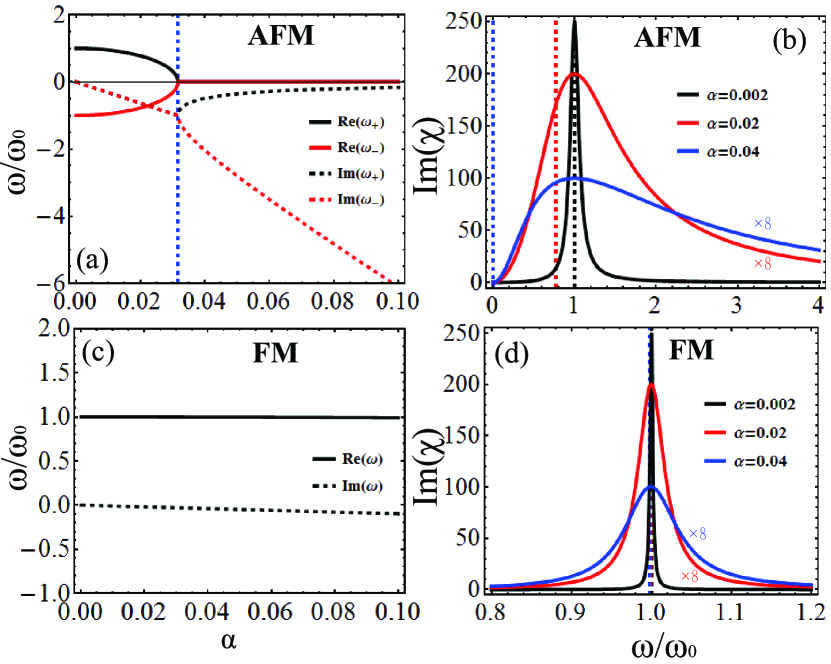
Figure 5: (a) Eigen-frequencies as a function of damping. The blue dashed line denotes the position of critical damping $\alpha_{c}$. (b) Absorption spectrum as a function of frequency when $\alpha=0.002$ (black line), 0.02 (red line), 0.04 (blue line), respectively. The dashed lines indicate the positions of the true resonance frequency ($\omega_{r}$) at the corresponding damping. (c) and (d) are the results for ferromagnets.

To resolve this anomaly, we first notice that the width of lineshape in Fig. 5(b) has become comparable to the resonance frequency when $\alpha$ is close to $\alpha_{c}$. This suggests that the quality factor ($Q$) of the resonance is very small and thus the lineshape is not reliable any longer. To see this point clearly, we can solve the half-maximum width of lineshape $\Delta\omega=4\alpha JS/(1+\alpha^{2})$ by setting $\omega=\omega_{m}$ in Eq. (14) and derive the $Q$ value as,

$$Q=\frac{\omega_{m}}{\Delta\omega}=\frac{\alpha_{c}(1+\alpha^{2})}{2\alpha}\approx\frac{\alpha_{c}}{2\alpha}.$$ (17)

At $\alpha=\alpha_{c}$, $Q=1/2$ is very bad. This effect is intrinsic for all types of antiferromagnets, no matter the quality of the sample is high or not. As a comparison, we can derive $Q=1/(2\alpha)$ for a ferromagnet, which does not suffer from this problem as long as $\alpha\ll 1$, as shown in Fig. 5(c) and 5(d).

Material	$H_{E}(T)$	$H_{\mathrm{sp}}(T)$	$\alpha_{c}$	$\mathrm{Exp.}$ $\alpha$
$\mathrm{NiO}\cite[cite]{\@@bibref{Authors Phrase1YearPhrase2}{Moriyama2018}{\@@citephrase{(}}{\@@citephrase{)}}}$	524	39	0.07	$5\times 10^{-4}$
$\mathrm{MnO}\cite[cite]{\@@bibref{Authors Phrase1YearPhrase2}{Sievers1963}{\@@citephrase{(}}{\@@citephrase{)}}}$	127	29	0.23	$<0.02$
$\mathrm{MnF_{2}}$ Johnson1959 ; Kotthaus1972	55.6	9.75	0.18	$6\times 10^{-4}$
$\alpha$-$\mathrm{Fe_{2}O_{3}}\cite[cite]{\@@bibref{Authors Phrase1YearPhrase2}{Lebrun2019}{\@@citephrase{(}}{\@@citephrase{)}}}$	1040	6	0.006	NA
$\mathrm{LaMnO_{3}}\cite[cite]{\@@bibref{Authors Phrase1YearPhrase2}{Talbayev2004}{\@@citephrase{(}}{\@@citephrase{)}}}$	33.9	5.2	0.15	NA
$\mathrm{Na_{4}^{3+}cluster}\cite[cite]{\@@bibref{Authors Phrase1YearPhrase2}{Nakano2013}{\@@citephrase{(}}{\@@citephrase{)}}}$	290	2.7	0.009	NA
$\mathrm{MnTe}\cite[cite]{\@@bibref{Authors Phrase1YearPhrase2}{Kriegner2017}{\@@citephrase{(}}{\@@citephrase{)}}}$	336	0.5	0.0015	NA
$\mathrm{Mn_{2}Au}\cite[cite]{\@@bibref{Authors Phrase1YearPhrase2}{Barthem2013}{\@@citephrase{(}}{\@@citephrase{)}}}$	1300	5	0.004	NA
$\gamma$-$\mathrm{MnCu}\cite[cite]{\@@bibref{Authors Phrase1YearPhrase2}{Wiltshire1983}{\@@citephrase{(}}{\@@citephrase{)}}}$	377	13	0.034	0.78

Table 2: List of the critical damping in commonly used antiferromagnets. Note that the exchange fields have different definitions in these references, here we only estimate the order of $\alpha_{c}$ as $H_{\mathrm{sp}}/H_{E}$ for simplicity. NA is short for “Not Applicable” and is used when no experimental values of dampings are found.

Physically, this difference between antiferromagnets and ferromagnets comes from their different dissipation mechanism. For an antiferromagnet, the magnetic moments on the two sublattices must tilt away from antiparallel orientations to launch the dissipation, while the antiferromagnetic exchange coupling ($H_{E}$) tends to suppress this tendency. As the exchange coupling becomes large, this channel will become highly un-efficient, therefore the resonant precession will be suppressed. For a ferromagnet, one magnetic moment simply dissipates through the Gilbert damping. The value of damping uniquely determines the speed of dissipation.

For reference, we summarize the typical values of critical dampings in Table 2 that include antiferromagnetic insulators, semiconductors and metals. They range from $10^{-3}$ to $10^{-1}$. For most of antiferromagnetic insulators, the intrinsic damping is expected to be smaller than $10^{-3}$, from the experience of magnetic resonance. Hence they should be well below the critical damping and antiferromagnetic resonance is still a reliable technique to extract magnetic parameters. For antiferromagnetic metals, the situation becomes worse since the critical damping is considerably large compared with the real damping and the resulting lineshape may deviate significantly from the Lorentz shape. This sets an intrinsic difficulty to analyze the resonance signal and it is probably the reason why very few resonant experiments are available for antiferromagnetic metals.

IV Discussions and conclusions

Here we would like to comment on the conventional wisdom of AFM community. It was taken for granted that MI in AFMs is negligible without any proof. Thus MI is neglected in most, if not all, of the analytical models, numerical simulations and in the analysis of AFM experimental results. Hence it is not surprising that results found here were not predicted early. Of course, MI naturally exists in experiments, and one should be very careful to explain the experimental data by the theory without MI effects, especially when extracting the anisotropy coefficients.

In conclusion, we have studied MI effects on the antiferromagnetic dynamics. Even though the total magnetic charges of an AFM as well as the resulting magnetostatic field outside the system are vanishingly small, the local charge distribution at atomic scale could considerably modify the system anisotropy in magnetic nanowires as well in quasi 2D and 3D structures. By analytically evaluating the effective dipolar anisotropy, we find that MI could even change the easy-axis of an properly designed nano-structure. We found that the switching time first decreases and then increases with the damping. The underdamped and overdamped phases are thus classified, resembling the motion of a non-linear pendulum. Near the phase boundary, the lineshape of AFM resonance becomes non-Lorentz with very low quality factor and thus it is not reliable any more to extract the magnetic parameters in this case.

V acknowledgments

HYY acknowledge Jiang Xiao for helpful discussions. The work is financially supported by National Natural Science Foundation of China (NSFC) under Grant No. 61704071 and Shenzhen Fundamental Subject Research Program under Grant No. JCYJ20180302174248595. MHY acknowledges support by Guangdong Innovative and Entrepreneurial Research Team Program (2016ZT06D348), and Science, Technology and Innovation Commission of Shenzhen Municipality (ZDSYS20170303165926217 and JCYJ20170412152620376). XRW was supported by the NSFC Grant (No. 11774296) as well as Hong Kong RGC Grants (Nos. 16301518, 16301619 and 16300117).

References

- (1) P. Wadley et al., Science 351, 587 (2016).
- (2) J. Železný, H. Gao, K.Výborný, J. Zemen, J. Mašek, A. Manchon, J. Wunderlich, J. Sinova, and T.Jungwirth, Phys. Rev. Lett. 113, 157201 (2014).
- (3) Q. Liu, H.Y. Yuan, K. Xia, and Z. Yuan, Phys. Rev. Mater. 1, 061401(R) (2017).
- (4) H.Y. Yuan, Q. Liu, K. Xia, Z. Yuan and X.R. Wang, EPL 126, 67006 (2019)..
- (5) A. V. Kimel, A. Kirilyuk, A. Tsvetkov, R. V. Pisarev, and Th. Rasing, Nature(London) 429, 850 (2004).
- (6) R. A. Duine, P. M. Haney, A. S. Nunez, and A. H. MacDonald, Phys. Rev. B 75, 014433 (2007).
- (7) P. M. Haney and A. H. MacDonald, Phys. Rev. Lett. 100, 196801 (2008).
- (8) Y. Xu, S. Wang, and K. Xia, Phys. Rev. Lett. 100, 226602 (2008).
- (9) R. Cheng, J. Xiao, Q. Niu, and A. Brataas, Phys. Rev. Lett. 113, 057601 (2014).
- (10) K. M. D. Hals, Y. Tserkovnyak, and A. Brataas, Phys. Rev. Lett. 106, 107206 (2011).
- (11) O. Gomonay, T. Jungwirth, and J. Sinova, Phys. Rev. Lett. 117, 017202 (2016).
- (12) T. Shiino, S.H. Oh, P.M. Haney, S.-W. Lee, G. Go, B.-G. Park, and K.-J. Lee, Phys. Rev. Lett. 117, 087203 (2016).
- (13) S. Selzer, U. Atxitia, U. Ritzmann, D. Hinzke, and U. Nowak, Phys. Rev. Lett. 117, 107201 (2016).
- (14) T. Jungwirth, X. Marti, P. Wadley, and J. Wunderlich, Nat. Nanotech. 11, 231 (2016).
- (15) X. Zhang, Y. Zhou, and M. Ezawa, Sci. Rep. 6, 24795 (2016).
- (16) J. Barker and O. A. Tretiakov, Phys. Rev. Lett. 116, 147203 (2016).
- (17) H. Y. Yuan, W. Wang, Man-Hong Yung, and X.R. Wang, Phys. Rev. B 97, 214434 (2018).
- (18) H. Y. Yuan, Man-Hong Yung, and X.R. Wang, Phys. Rev. B 98, 060407(R) (2018).
- (19) H. V. Gomonay and V. M. Loktev, Phys. Rev. B 81, 144427 (2010).
- (20) M. J. Stephen and J. P. Straley, Red. Mod. Phys. 46, 617 (1974).
- (21) A. Vansteenkiste, J. Leliaert, M. Dvornik, M. Helsen, F. Garcia-Sanchez, and B. Van Waeyenberge, The design and verification of MuMax3, AIP Adv. 4 107133 (2014).
- (22) A. A. Sapozhnik, C. Luo, H. Ryll, F. Radu, M. Jourdan, H. Zabel, and H.-J. Elmers, arxiv:1803.03524v1.
- (23) A. B. Shick, S. Khmelevskyi, O. N. Mryasov, J. Wunderlich, and T. Jungwirth, Phys. Rev. B 81, 212409 (2010).
- (24) A. J. Newell, W. Williams, and D. J. Dunlop, J. Geophys. Res. 98, 9551 (1993).
- (25) J. D. Jackson, Classical Electrodynamics, Ed. (John Wiley, 1998)
- (26) M. Weisheit, S. Fähler, A. Marty, Y. Souche, C. Poinsignon, and D. Givord, Science 315, 349 (2007).
- (27) T. Maruyama, Y. Shiota1, T. Nozaki, K. Ohta, N. Toda, M. Mizuguchi, A. A. Tulapurkar, T. Shinjo, M. Shiraishi, S. Mizukami, Y. Ando, and Y. Suzuki, Nat. Nanotech. 4, 158 (2009).
- (28) D. Lebeugle, A. Mougin, M. Viret, D. Colson, and L. Ranno, Phys. Rev. Lett. 103, 257601 (2009).
- (29) K. Johannessen, Eur. J. Phys. 35, 035014 (2014).
- (30) Y. Zhang, H. Y. Yuan, X. S. Wang, and X. R. Wang, Phys. Rev. B 97, 144416 (2018).
- (31) For a ferromagnet, we can follow a simialr approach in Sec. IIA and derive .
- (32) Weiwei Wang, C. Gu, Y. Zhou, and H. Fangohr, Phys. Rev. B 96, 024430 (2017).
- (33) H. Y. Yuan and X. R. Wang, Appl. Phys. Lett. 110, 082403 (2017).
- (34) Y. Zhang, X. S. Wang, H. Y. Yuan, S. S. Kang, H. W. Zhang, and X. R. Wang, J Phys.: Condens. Mater 29, 095806 (2017).
- (35) One can analyticall obtain by solving the equation .
- (36) T. Moriyama, K. Hayashi, K. Yamada, M. Shima, Y. Ohya, and T. Ono, Phys. Rev. Mater. 3, 051402 (R) (2019).
- (37) A. J. Sievers and M. Tinkham, Phys. Rev. 129, 1566 (1963).
- (38) F. M. Johnson and A. H. Nethercot, Phys. Rev. 114, 705 (1959).
- (39) J. P. Kotthaus and V. Jaccarino, Phys. Rev. Lett. 28, 1649 (1972).
- (40) R. Lebrun, A. Ross, O. Gomonay, S. A. Bender, L. Baldrati, F. Kronast, A. Qaiumzadeh, J. Sinova, A. Brataas, R. A. Duine and M. Klaui, Commun. Phys. 2, 50 (2019).
- (41) D. Talbayev, L. Mihaly, and J. Zhou, Phys. Rev. Lett. 93, 017202 (2004).
- (42) T. Nakano, H. Tsugeno, A. Hanazawa, T. Kashiwagi, Y. Nozue, and M. Hagiwara, Phys. Rev. B 88, 174401 (2013).
- (43) D. Kriegner et al., Phys. Rev. B 96, 214418 (2017). Here we estimate the exchange field from the Néel temperature of MnTe.
- (44) V.M.T.S. Barthem, C.V. Colin, H. Mayaffre, M.-H. Julien, and D. Givord, Nat. Commun. 4, 2892 (2013).
- (45) M.C.K. Wiltshire and M. M. Elcombe, Physica 120B, 167 (1983).