On the shift-invert Lanczos method for
the buckling eigenvalue problem

Abstract

We consider the problem of extracting a few desired eigenpairs of the buckling eigenvalue problem $Kx=\lambda K_{G}x$, where $K$ is symmetric positive semi-definite, $K_{G}$ is symmetric indefinite, and the pencil $K-\lambda K_{G}$ is singular, namely, $K$ and $K_{G}$ share a non-trivial common nullspace. Moreover, in practical buckling analysis of structures, bases for the nullspace of $K$ and the common nullspace of $K$ and $K_{G}$ are available. There are two open issues for developing an industrial strength shift-invert Lanczos method: (1) the shift-invert operator $(K-\sigma K_{G})^{-1}$ does not exist or is extremely ill-conditioned, and (2) the use of the semi-inner product induced by $K$ drives the Lanczos vectors rapidly towards the nullspace of $K$, which leads to a rapid growth of the Lanczos vectors in norms and cause permanent loss of information and the failure of the method. In this paper, we address these two issues by proposing a generalized buckling spectral transformation of the singular pencil $K-\lambda K_{G}$ and a regularization of the inner product via a low-rank updating of the semi-positive definiteness of $K$. The efficacy of our approach is demonstrated by numerical examples, including one from industrial buckling analysis.

Keywords: Eigenvalue problem, buckling analysis, Lanczos method, singular pencil

Mathematics Subject Classifications: 65F15, 15A18

1 Introduction

We consider the buckling eigenvalue problem

$$Kx=\lambda K_{G}x,$$ (1.1)

where $K$ and $K_{G}$ are $n\times n$ symmetric matrices, and $K$ is positive semi-definite and $K_{G}$ is indefinite. Furthermore, the pencil $K-\lambda K_{G}$ is singular, i.e., the matrices $K$ and $K_{G}$ share a nontrivial common nullspace $\mathcal{Z}_{c}$. We are interested in (i) extracting a few nonzero finite eigenvalues around a prescribed shift $\sigma\neq 0$ and the associated eigenvectors $x$ perpendicular to the common nullspace $\mathcal{Z}_{c}$, and (ii) counting the number of eigenvalues of $K-\lambda K_{G}$ in a given interval $(\alpha,\beta)$. As in practical buckling analysis of structures, we assume that a basis $Z\equiv[Z_{N}\ Z_{C}]$ of the nullspace of $K$ and a basis $Z_{C}$ of the common nullspace $\mathcal{Z}_{c}$ of $K$ and $K_{G}$ are available, and the pencil $K-\lambda K_{G}$ is simultaneously diagonalizable.

The buckling eigenvalue problem (1.1) arises from the buckling analysis in structural engineering, where $K$ is referred to as the stiffness matrix and $K_{G}$ is referred to as the geometric stiffness matrix. The eigenvalue $\lambda$ is used to determine the critical load at which a structure may become unstable [18, p. 72], and the eigenvector $x$ is the associated buckling shape. The bases for the nullspace of $K$ and the common nullspace $\mathcal{Z}_{c}$ of $K$ and $K_{G}$ can be extracted from the algebraic or geometric structure of the problem [10, 23].

The buckling eigenvalue problem (1.1) remains an outstanding computational challenge in numerical linear algebra [20, 28] and in industrial applications [14]. When the pencil $K-\lambda K_{G}$ is regular and $K$ is positive definite, a common practice for computing eigenpairs around a given shift $\sigma$ is to convert (1.1) into the following ordinary eigenproblem via a so-called buckling spectral transformation

$$(K-{\sigma}K_{G})^{-1}Kx=\frac{\lambda}{{\lambda}-{\sigma}}x,$$ (1.2)

see [8, 22, 15, 19]. Since $(K-{\sigma}K_{G})^{-1}K$ is symmetric with respect to $K$, the Lanczos method with $K$-inner product can be immediately used to solve the eigenproblem (1.2). This approach is referred to as the shift-invert Lanczos method and has been widely used, including in a number of industrial strength eigensolvers, such as LS-DYNA [14].

However, when $K$ is positive semi-definite and $K-{\lambda}K_{G}$ is singular, we have the following two issues:

1. Since the pencil $K-\lambda K_{G}$ is singular or near singular, i.e., the matrices $K$ and $K_{G}$ share a non-trivial common nullspace $\mathcal{Z}_{c}$, the shift-invert matrix $(K-\sigma K_{G})^{-1}$ does not exist or is extremely ill-conditioned.

2. Since the matrix $K$ is positive semi-definite, the inner product induced by $K$ causes the Lanczos vectors driven rapidly toward the nullspace of $K$ [22, 21, 20, 28]. It results in the large norms of the Lanczos vectors, which introduces large rounding errors. The accuracy of the computed solutions is degraded and even failed.

These issues have been studied since the early development of the shift-invert Lanczos method in the 1980s. Nour-Omid et al. [22] proposed a modified formulation of the Ritz vectors to refine the computed solutions. Meerbergen [20] proposed to control the norms of the Lanczos vectors by applying implicit restart [27]. More recently, Stewart [28] gave a detailed analysis to show that the loss of information caused by the growth of the Lanczos vectors is permanent.

In this paper, we address the two issues by first proposing a generalized buckling spectral transformation of the singular pencil $K-\lambda K_{G}$, and a reguarlization of the inner product via a low-rank updating of the positive semi-definite matrix $K$. Then a shift-invert Lanczos method for the buckling eigenvalue problem (1.1) is developed. We will discuss two implementations of the matrix-vector product for the computational kernel of the shift-invert Lanczos method, and propose two ways to count the number of eigenvalues in a given interval $(\alpha,\beta)$ for validation.

The rest of the paper is organized as follows. In §2, we first present a canonical form of the pencil $K-\lambda K_{G}$, and propose a generalized buckling spectral transformation, and a regularization of the inner product. In §3, we discuss the implementation of the shift-invert Lanczos method with the generalized buckling spectral transformation and the regularized inner product. In §4, we discuss two ways to count the number of eigenvalues in an interval. Efficacy of the proposed approach is demonstrated in §5. Concluding remarks are given in §6.

Following the convention of matrix computations, we use the upper case letters for matrices and lower case letters for vectors. In particular, we use $I_{n}$ for the identity matrix of dimension $n$ with $e_{j}$ being the $j$th column. If not specified, the dimensions of matrices and vectors conform to the dimensions used in the context. $\cdot^{T}$ is for transpose, $\cdot^{\dagger}$ for pseudo-inverse, $\|\cdot\|_{1}$ for $1$-norm, and $\|\cdot\|_{2}$ and $\|\cdot\|_{F}$ for $2$-norm and Frobenius norm, respectively. Also, we use $A^{-T}$ for the inverse of the matrix $A^{T}$. The range and the nullspace of a matrix $A$ are denoted by $\mathcal{R}(A)$ and $\mathcal{N}(A)$, respectively. The direct sum of two subspaces $\mathcal{S}_{1}$ and $\mathcal{S}_{2}$ is denoted by $\mathcal{S}_{1}\oplus\mathcal{S}_{2}$. The orthogonal complement to a subspace $\mathcal{S}$ is denoted by $\mathcal{S}^{\perp}$ and the orthogonal projection onto a subspace $\mathcal{S}$ is denoted by $\mathcal{P}_{\mathcal{S}}$. $\nu_{+}(S)$, $\nu_{-}(S)$ and $\nu_{0}(S)$ denote the positive, negative and zero eigenvalues of a symmetric matrix $S$, respectively. Other notations will be explained as used.

2 Theory

2.1 Canonical form

We start with a canonical form of the pencil $K-\lambda K_{G}$. For the compactness of presentation, we interchange the roles of $K$ and $K_{G}$ in (1.1) and consider the reversal of the pencil $K-{\lambda}K_{G}$, i.e., $K_{G}-{\lambda}^{\#}K$.

Theorem 1.

For the pencil $K_{G}-{\lambda}^{\#}K$, there exists a non-singular matrix $W\in{\mathbb{R}}^{n\times n}$ such that

$$W^{T}K_{G}W=\hbox{}\vbox{\kern 0.86108pt\hbox{$\kern 0.0pt\kern 2.5pt\kern-5.0pt\left[\kern 0.0pt\kern-2.5pt\kern-5.55557pt\vbox{\kern-0.86108pt\vbox{\vbox{ \halign{\kern\arraycolsep\hfil\@arstrut$\kbcolstyle#$\hfil\kern\arraycolsep& \kern\arraycolsep\hfil$\@kbrowstyle#$\ifkbalignright\relax\else\hfil\fi\kern\arraycolsep&& \kern\arraycolsep\hfil$\@kbrowstyle#$\ifkbalignright\relax\else\hfil\fi\kern\arraycolsep\cr 5.0pt\hfil\@arstrut$\scriptstyle$\hfil\kern 5.0pt&5.0pt\hfil$\scriptstyle n_{1}$\hfil\kern 5.0pt&5.0pt\hfil$\scriptstyle n_{2}$\hfil\kern 5.0pt&5.0pt\hfil$\scriptstyle n_{3}\\n_{1}$\hfil\kern 5.0pt&5.0pt\hfil$\scriptstyle{\Lambda}^{\#}_{1}$\hfil\kern 5.0pt&5.0pt\hfil$\scriptstyle$\hfil\kern 5.0pt&5.0pt\hfil$\scriptstyle\\n_{2}$\hfil\kern 5.0pt&5.0pt\hfil$\scriptstyle$\hfil\kern 5.0pt&5.0pt\hfil$\scriptstyle{\Lambda}^{\#}_{2}$\hfil\kern 5.0pt&5.0pt\hfil$\scriptstyle\\n_{3}$\hfil\kern 5.0pt&5.0pt\hfil$\scriptstyle$\hfil\kern 5.0pt&5.0pt\hfil$\scriptstyle$\hfil\kern 5.0pt&5.0pt\hfil$\scriptstyle 0$\hfil\kern 5.0pt\crcr}}}}\right]$}}\quad\mbox{and}\quad W^{T}KW=\hbox{}\vbox{\kern 0.86108pt\hbox{$\kern 0.0pt\kern 2.5pt\kern-5.0pt\left[\kern 0.0pt\kern-2.5pt\kern-5.55557pt\vbox{\kern-0.86108pt\vbox{\vbox{ \halign{\kern\arraycolsep\hfil\@arstrut$\kbcolstyle#$\hfil\kern\arraycolsep& \kern\arraycolsep\hfil$\@kbrowstyle#$\ifkbalignright\relax\else\hfil\fi\kern\arraycolsep&& \kern\arraycolsep\hfil$\@kbrowstyle#$\ifkbalignright\relax\else\hfil\fi\kern\arraycolsep\cr 5.0pt\hfil\@arstrut$\scriptstyle$\hfil\kern 5.0pt&5.0pt\hfil$\scriptstyle n_{1}$\hfil\kern 5.0pt&5.0pt\hfil$\scriptstyle n_{2}$\hfil\kern 5.0pt&5.0pt\hfil$\scriptstyle n_{3}\\n_{1}$\hfil\kern 5.0pt&5.0pt\hfil$\scriptstyle I_{n_{1}}$\hfil\kern 5.0pt&5.0pt\hfil$\scriptstyle$\hfil\kern 5.0pt&5.0pt\hfil$\scriptstyle\\n_{2}$\hfil\kern 5.0pt&5.0pt\hfil$\scriptstyle$\hfil\kern 5.0pt&5.0pt\hfil$\scriptstyle 0$\hfil\kern 5.0pt&5.0pt\hfil$\scriptstyle\\n_{3}$\hfil\kern 5.0pt&5.0pt\hfil$\scriptstyle$\hfil\kern 5.0pt&5.0pt\hfil$\scriptstyle$\hfil\kern 5.0pt&5.0pt\hfil$\scriptstyle 0$\hfil\kern 5.0pt\crcr}}}}\right]$}},$$ (2.1)

where ${\Lambda}^{\#}_{1}$ and ${\Lambda}^{\#}_{2}$ are diagonal matrices with real diagonal entries, and ${\Lambda}^{\#}_{2}$ is non-singular. Furthermore, by conformally partitioning $W=[W_{1},W_{2},W_{3}]$, we have

$$W_{3}^{T}W_{1}=0\quad\mbox{and}\quad W_{3}^{T}W_{2}=0,$$ (2.2)

Proof.

see Appendix A. ∎

Remark 1.

By the canonical form (2.1), we immediately know that (i) the columns of $W_{3}$ span the common nullspace $\mathcal{Z}_{c}$ of $K$ and $K_{G}$, and the columns of $[W_{1}\ W_{2}]$ span the orthogonal complement to $\mathcal{Z}_{c}$, i.e., $\mathcal{Z}_{c}^{\perp}$; (ii) the columns of $W_{1}$ are eigenvectors associated with real finite eigenvalues $({\Lambda}^{\#}_{1},I_{n_{1}})$ of the pencil $K_{G}-{\lambda}^{\#}K$ and are perpendicular to $\mathcal{Z}_{c}$; (iii) The columns of $W_{2}$ are eigenvectors associated with an infinite eigenvalue $({\Lambda}^{\#}_{2},0)$ of the pencil $K_{G}-{\lambda}^{\#}K$ and are perpendicular to $\mathcal{Z}_{c}$; (iv) For $x\in\mathcal{Z}_{c}$, $({\lambda}^{\#},x)$ is an eigenpair of the pencil $K_{G}-{\lambda}^{\#}K$ for any ${\lambda}^{\#}\in{\mathbb{C}}$.

2.2 Generalized buckling spectral transformation

Mathematically, the generalized buckling spectral transformation of the singular pencil $K-\lambda K_{G}$ is to replace the inverse in (1.2) by the pseudo-inverse and leads to the ordinary eigenvalue problem

$$Cx=\mu x\quad\mbox{and}\quad C=(K-\sigma K_{G})^{\dagger}K,$$ (2.3)

where $(K-\sigma K_{G})^{\dagger}$ is the pseudo-inverse of the singular matrix $K-\sigma K_{G}$ [13, p. 290]. Note that the non-zero real shift $\sigma$ cannot be an eigenvalue of the pencil $K-\lambda K_{G}$.

The following theorem provides the relationship of non-trivial eigenpairs between the original buckling eigenvalue problem (1.1) and the ordinary eigenvalue problem (2.3).

Theorem 2.

$(\lambda,x)$ is an eigenpair of the pencil $K-\lambda K_{G}$ with non-zero finite eigenvalue $\lambda$ and $x\in\mathcal{Z}_{c}^{\perp}$ if and only if $(\mu,x)$ is an eigenpair of the matrix $C$ in (2.3) with $\mu\neq 0$ and $\mu\neq 1$ and $x\in\mathcal{Z}_{c}^{\perp}$, where $\mu=\frac{\lambda}{\lambda-\sigma}$ and $\sigma\neq 0$.

Before proving Theorem 2, we use the canonical form (2.1) to derive an eigenvalue decomposition of $C$ and prove the eigenvalue and eigenvector relations between $K_{G}-\lambda^{\#}K$ and $C$.

Lemma 1.

With the canonical form (2.1) in Theorem 1, an eigenvalue decomposition of the matrix $C$ defined in (2.3) is given by

$$CW=W\left[\begin{array}[]{ccc}(I_{n_{1}}-\sigma{\Lambda}^{\#}_{1})^{-1}&&\\ &0&\\ &&0\end{array}\right].$$ (2.7)

Proof.

Recall that, since the matrix $K-\sigma K_{G}$ is symmetric,

$$\mathcal{R}(K-\sigma K_{G})=\mathcal{N}(K-\sigma K_{G})^{\perp}=\mathcal{Z}_{c}^{\perp}.$$ (2.8)

In addition, by the condition (2.2) in the canonical form (2.1), we have

$$\mathcal{R}(W_{1})\oplus\mathcal{R}(W_{2})=\mathcal{R}(W_{3})^{\perp}=\mathcal{Z}_{c}^{\perp}.$$ (2.9)

Therefore, from (2.8) and (2.9),

$$\mathcal{R}(K-\sigma K_{G})=\mathcal{R}(W_{1})\oplus\mathcal{R}(W_{2})=\mathcal{R}(W_{3})^{\perp}=\mathcal{Z}_{c}^{\perp}.$$ (2.10)

Now note that, from the canonical form (2.1),

$$W^{T}KW=\left[\begin{array}[]{ccc}I_{n_{1}}&&\\ &0&\\ &&0\end{array}\right]\quad\mbox{and}\quad W^{T}(K-\sigma K_{G})W=\left[\begin{array}[]{ccc}I_{n_{1}}-\sigma{\Lambda}^{\#}_{1}&&\\ &-\sigma{\Lambda}^{\#}_{2}&\\ &&0\end{array}\right].$$ (2.17)

Therefore we have

$$W^{T}KW=\left[\begin{array}[]{ccc}I_{n_{1}}&&\\ &0&\\ &&0\end{array}\right]=W^{T}(K-\sigma K_{G})W\left[\begin{array}[]{ccc}(I_{n_{1}}-\sigma{\Lambda}^{\#}_{1})^{-1}&&\\ &0&\\ &&0\end{array}\right].$$ (2.24)

Left multiplying (2.24) by $W^{-T}$, it yields that

$$KW=(K-\sigma K_{G})W\left[\begin{array}[]{ccc}(I_{n_{1}}-\sigma{\Lambda}^{\#}_{1})^{-1}&&\\ &0&\\ &&0\end{array}\right].$$ (2.28)

From the Moore-Penrose conditions [13, p. 290],

$$(K-\sigma K_{G})^{\dagger}(K-\sigma K_{G})=\mathcal{P}_{\mathcal{R}((K-\sigma K_{G})^{T})}=\mathcal{P}_{\mathcal{R}(K-\sigma K_{G})},$$ (2.29)

namely $(K-\sigma K_{G})^{\dagger}(K-\sigma K_{G})$ is an orthogonal projection onto ${\mathcal{R}((K-\sigma K_{G})^{T})}={\mathcal{R}(K-\sigma K_{G})}$. Therefore, from (2.10) and (2.29),

$$(K-\sigma K_{G})^{\dagger}(K-\sigma K_{G})W=W\left[\begin{array}[]{ccc}I_{n_{1}}&&\\ &I_{n_{2}}&\\ &&0\end{array}\right].$$ (2.33)

Left multiplying (2.28) by $(K-\sigma K_{G})^{\dagger}$ and using (2.33), we have the eigenvalue decomposition (2.7) of $C$. ∎

Lemma 2.

The matrix $C$ defined in (2.3) has the following properties:

• $({\lambda}^{\#},x)$ is an eigenpair of $K_{G}-{\lambda}^{\#}K$ with non-zero finite ${\lambda}^{\#}$ and $x\in\mathcal{Z}_{c}^{\perp}$ if and only if $(\mu,x)$ is an eigenpair of $C$ with $\mu\neq 0$ and $\mu\neq 1$ and $x\in\mathcal{Z}_{c}^{\perp}$, where $\mu=\frac{1}{1-\sigma{\lambda}^{\#}}$.

• $({\lambda}^{\#},x)$ is an eigenpair of $K_{G}-{\lambda}^{\#}K$ with ${\lambda}^{\#}=0$ and $x\in\mathcal{Z}_{c}^{\perp}$ if and only if $(\mu,x)$ is an eigenpair of $C$ with $\mu=1$ and $x\in\mathcal{Z}_{c}^{\perp}$.

• $({\lambda}^{\#},x)$ is an eigenpair of $K_{G}-{\lambda}^{\#}K$ with $|{\lambda}^{\#}|=\infty$ and $x\in\mathcal{Z}_{c}^{\perp}$ if and only if $(\mu,x)$ is an eigenpair of $C$ with $\mu=0$ and $x\in\mathcal{Z}_{c}^{\perp}$.

• If $x\in\mathcal{Z}_{c}$, $Cx=0$.

Proof.

The lemma can be proved by comparing the eigenvalue decomposition (2.7) of $C$ with the canonical form (2.1) of $K_{G}-{\lambda}^{\#}K$. Specifically, for (i) and (ii), recall that each column of $W_{1}$ is an eigenvector associated with a real, finite eigenvalue ${\lambda}^{\#}$ of the pencil $K_{G}-{\lambda}^{\#}K$ and the eigenvector is perpendicular to the common nullspace $\mathcal{Z}_{c}$. From (2.7), each column of $W_{1}$ is now an eigenvector associated with a non-zero, finite eigenvalue $\mu=(1-\sigma{\lambda}^{\#})^{-1}$ of the eigenproblem (2.3).

To show (iii), recall that each column of $W_{2}$ is an eigenvector associated with an infinite eigenvalue of the pencil $K_{G}-{\lambda}^{\#}K$ and the eigenvector is perpendicular to the common nullspace $\mathcal{Z}_{c}$. From (2.7), each column of $W_{2}$ is now an eigenvector associated with zero eigenvalue of the eigenproblem (2.3).

Finally, for (iv), the common nullspace $\mathcal{Z}_{c}$ is spanned by the columns of $W_{3}$ and, from (2.7), we know that $Cx=0$ if $x\in\mathcal{Z}_{c}$. ∎

Proof of Theorem 2. Note that $(\lambda,x)$ is an eigenpair of $K-\lambda K_{G}$ with non-zero finite eigenvalue $\lambda$ and $x\in\mathcal{Z}_{c}^{\perp}$ if and only if $({\lambda}^{\#},x)$ is an eigenpair of $K_{G}-{\lambda}^{\#}K$ with non-zero finite eigenvalue ${\lambda}^{\#}=\lambda^{-1}$ and $x\in\mathcal{Z}_{c}^{\perp}$. Also, from Lemma 1(i), we know that $({\lambda}^{\#},x)$ is an eigenpair of $K_{G}-{\lambda}^{\#}K$ with non-zero finite eigenvalue ${\lambda}^{\#}$ and $x\in\mathcal{Z}_{c}^{\perp}$ if and only if $(\mu,x)$ is an eigenpair of the eigenvalue problem $Cx=\mu x$ with $\mu=\frac{1}{1-\sigma{\lambda}^{\#}}$, $\mu\neq 0$ and $\mu\neq 1$, and $x\in\mathcal{Z}_{c}^{\perp}$. Therefore, $(\lambda,x)$ is an eigenpair of the pencil $K-\lambda K_{G}$ with non-zero finite eigenvalue $\lambda$ and $x\in\mathcal{Z}_{c}^{\perp}$ if and only if $(\mu,x)$ is an eigenpair of the eigenvalue problem $Cx=\mu x$ with $\mu=\frac{\lambda}{\lambda-\sigma}$, $\mu\neq 0$ and $\mu\neq 1$, and $x\in\mathcal{Z}_{c}^{\perp}$. $\Box$

By Theorem 2, near the shift $\sigma$, the eigenpairs $(\lambda,x)$ of $K-\lambda K_{G}$ with non-zero finite eigenvalues $\lambda$ and $x\in\mathcal{Z}_{c}^{\perp}$ are transformed into eigenpairs $(\mu,x)$ of $C$ with non-zero eigenvalues $\mu$, which typically are well-separated, and those away from the shift $\sigma$ are transformed into clustered eigenpairs $(\mu,x)$ of $C$ near unity as shown in Figure 2.1. We note that the eigenpairs $(\mu,x)$ with $\mu=0$ or $\mu=1$ are not the ones of interest. The eigenpairs $(1,x)$ correspond to eigenpairs of $K-\lambda K_{G}$ with infinite eigenvalues and the eigenpairs $(0,x)$ correspond to eigenpairs of $K-\lambda K_{G}$ with $x\in\mathcal{N}(K)$.

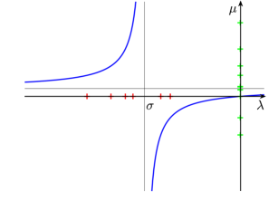
Figure 2.1: Buckling spectral transfromation with $\sigma<0$ (left) and $\sigma>0$ (right).

2.3 Regularization of the inner product

In this subsection we introduce a positive definite matrix $M$ from a low-rank updating of $K$, and then show that the matrix $C$ in the generalized buckling spectral transformation (2.3) is symmetric with respect to the inner product induced by $M$.

Theorem 3.

Let $C$ be defined in (2.3). Let $Z=[Z_{N}\ Z_{C}]$ span the nullspace $\mathcal{N}(K)$ and $Z_{C}$ span the common nullspace $\mathcal{Z}_{c}$ of $K$ and $K_{G}$. Define

$$M=K+(K_{G}Z_{N})H_{N}(K_{G}Z_{N})^{T}+Z_{C}H_{C}Z_{C}^{T},$$ (2.34)

where $H_{N}$ and $H_{C}$ are arbitrary positive definite matrices. Then

• the matrix $M$ is positive definite,

• the matrix $C$ is symmetric with respect to the inner product induced by $M$.

Proof.

By the canonical form (2.1), we have

$$\mathcal{N}(K)=\mathcal{R}(W_{2})\oplus\mathcal{R}(W_{3})=\mathcal{R}(Z_{N})\oplus\mathcal{R}(Z_{C})\quad\mbox{and}\quad\mathcal{Z}_{c}=\mathcal{R}(W_{3})=\mathcal{R}(Z_{C}),$$

and

$$\left[\begin{array}[]{cc}Z_{N}&Z_{C}\end{array}\right]=\left[\begin{array}[]{cc}W_{2}&W_{3}\end{array}\right]\left[\begin{array}[]{cc}R_{22}&O\\ R_{32}&R_{33}\end{array}\right]$$

for some matrices $R_{22}\in{\mathbb{R}}^{n_{2}\times n_{2}}$, $R_{32}\in{\mathbb{R}}^{n_{3}\times n_{2}}$, $R_{33}\in{\mathbb{R}}^{n_{3}\times n_{3}}$, and $R_{22}$ and $R_{33}$ are non-singular. Therefore,

$$W^{T}K_{G}Z_{N}=W^{T}K_{G}(W_{2}R_{22}+W_{3}R_{32})=W^{T}K_{G}W_{2}R_{22}=\left[\begin{array}[]{c}0\\ {\Lambda}^{\#}_{2}R_{22}\\ 0\end{array}\right].$$

Since the basis $W$ satisfies the condition (2.2),

$$W^{T}Z_{C}=W^{T}W_{3}R_{33}=\left[\begin{array}[]{c}0\\ 0\\ (W_{3}^{T}W_{3})R_{33}\end{array}\right].$$

Therefore,

$$W^{T}MW=W^{T}\big{(}K+(K_{G}Z_{N})H_{N}(K_{G}Z_{N})^{T}+Z_{C}H_{C}Z_{C}^{T}\big{)}W=\begin{bmatrix}I_{n_{1}}&&\\ &\widehat{H}_{N}&\\ &&\widehat{H}_{C}\end{bmatrix},$$ (2.35)

where

$$\widehat{H}_{N}={\Lambda}^{\#}_{2}R_{22}H_{N}R_{22}^{T}{\Lambda}^{\#}_{2}\quad\mbox{and}\quad\widehat{H}_{C}=(W_{3}^{T}W_{3})R_{33}H_{C}R_{33}^{T}(W_{3}^{T}W_{3}).$$

To prove that $M$ is positive definite, we show that both $\widehat{H}_{N}$ and $\widehat{H}_{C}$ are positive definite. For the matrix $\widehat{H}_{N}$, we note that the matrix $H_{N}$ is positve definite and the matrix $R_{22}$ is non-singular. Also, from Theorem 1, the diagonal matrix ${\Lambda}^{\#}_{2}$ is non-singular. Therefore, the matrix $\widehat{H}_{N}$ is positive definite. For the matrix $\widehat{H}_{C}$, we note that the matrix $H_{C}$ is positive definite and the matrix $R_{33}$ is non-singular. Also, since the matrix $W_{3}$ is of full rank, the symmetric matrix $W_{3}^{T}W_{3}$ is non-singular. Therefore, the matrix $\widehat{H}_{C}$ is also positive definite. This proves $(i)$.

To prove $(ii)$, by the eigenvalue decomposition (2.7) of $C$ and (2.35), we have

$$W^{T}MCW=W^{T}MWW^{-1}CW=\left[\begin{array}[]{ccc}(I_{n_{1}}-\sigma{\Lambda}^{\#}_{1})^{-1}&&\\ &0&\\ &&0\end{array}\right].$$

Therefore, the matrix $MC$ is symmetric, which means that the matrix $C$ is symmetric with respect to the inner product induced by $M$. ∎

Remark 2.

We note that if the pencil $K-\lambda K_{G}$ is regular, Theorem 3 is still applicable. In this case, the matrix $C$ in (1.2) is symmetric with respect to the inner product induced by $M=K+(K_{G}Z_{N})H_{N}(K_{G}Z_{N})^{T}$.

3 Shift-invert Lanczos method

3.1 Shift-invert Lanczos method

By Theorem 2, we have generalized the buckling spectral transformation to the singular pencil $K-\lambda K_{G}$ and converted the buckling eigenproblem (1.1) into an equivalent ordinary eigenvalue problem (2.3). From Theorem 3, we know that the matrix $C$ in (2.3) is symmetric with respect to the inner product induced by the positive definite matrix $M$ in (2.34). It naturally leads that to solve the buckling eigenvalue problem (1.1), we can use the Lanczos method on the matrix $C$ with the inner product induced by $M$. This new strategy is also referred to as the shift-invert Lanczos method and outlined in Algorithm 1.

The shift-invert Lanczos method, after $j$ steps, computes a sequence of Lanczos vectors $\{v_{1}\ \ldots\ v_{j+1}\}$ and a symmetric tridiagonal matrix $T_{j}=\mbox{tridiag}(\beta_{i-1},\alpha_{i},\beta_{i})$ satisfying the governing equations

$$CV_{j}=V_{j}T_{j}+\beta_{j}v_{j+1}e_{j}^{T}\quad\mbox{and}\quad V_{j+1}^{T}MV_{j+1}=I_{j+1},$$ (3.1)

where $V_{j+1}\equiv[v_{1}\ \ldots\ v_{j+1}]$. Great cares must be taken to ensure that the equations in (3.1) are satisfied [25, 8, 26, 22, 15] in the presence of finite-precision arithmetic. Several techniques have been developed and well-implemented [25, 26, 15]. For the rest of discussion, we will focus on the implementations of the matrix-vector product $u=Cv$ for Line 6 of Algorithm 1.

Algorithm 1 Shift-invert Lanczos method for the buckling eigenvalue problem (1.1)

1:  $r\leftarrow v$, where $v$ is the starting vector

2:  $p\leftarrow Mr$, where $M=K+(K_{G}Z_{N})H_{N}(K_{G}Z_{N})^{T}+Z_{C}H_{C}Z_{C}^{T}$

3:  $\beta_{0}\leftarrow(p^{T}r)^{1/2}$

4:  for $j=1,2,\ldots$ do

5:     $v_{j}\leftarrow r/\beta_{j-1}$

6:     $r\leftarrow Cv_{j}$, where $C=(K-\sigma K_{G})^{\dagger}K$

7:     $r\leftarrow r-\beta_{j-1}v_{j-1}$

8:     $p\leftarrow Mr$

9:     $\alpha_{j}\leftarrow v_{j}^{T}p$

10:     $r\leftarrow r-\alpha_{j}v_{j}$

11:     perform re-orthogonalization if necessary

12:     $p\leftarrow Mr$

13:     $\beta_{j}\leftarrow(p^{T}r)^{1/2}$

14:     Compute the eigenvalue decomposition of $T_{j}$

15:     Check convergence

16:  end for

17:  Compute approximate eigenvectors of the converged eigenpairs

3.2 The matrix-vector product

We first show that the matrix-vector product $u=Cv=(K-\sigma K_{G})^{\dagger}Kv$ is connected with the solution of a consistent singular linear system with constraint. Based on this connection, we present two ways for computing the vector $u$.

Theorem 4.

Given $v\in{\mathbb{R}}^{n}$, the vector

$$u=(K-\sigma K_{G})^{\dagger}Kv$$ (3.2)

is the unique solution of the consistent singular linear system

$$(K-\sigma K_{G})u=Kv$$ (3.3)

with the constraint

$$Z_{C}^{T}u=0,$$ (3.4)

where $Z_{C}$ is a basis of the common nullspace of $K$ and $K_{G}$.

Proof.

First note that since both $K$ and $K-\sigma K_{G}$ are symmetric, we have

$$\mathcal{R}(K)=\mathcal{N}(K)^{\perp}\quad\mbox{and}\quad\mathcal{R}(K-\sigma K_{G})=\mathcal{N}(K-\sigma K_{G})^{\perp}=\mathcal{Z}_{c}^{\perp}$$ (3.5)

and

$$\mathcal{Z}_{c}=\mathcal{N}(K-\sigma K_{G})\subset\mathcal{N}(K).$$ (3.6)

Therefore from (3.5) and (3.6),

$$Kv\in\mathcal{R}(K)\subset\mathcal{R}(K-\sigma K_{G}),$$

which implies that the linear system (3.3) is consistent. From (3.2),

$$(K-\sigma K_{G})u=(K-\sigma K_{G})(K-\sigma K_{G})^{\dagger}Kv=\mathcal{P}_{\mathcal{R}(K-\sigma K_{G})}Kv=Kv,$$ (3.7)

where $\mathcal{P}_{\mathcal{R}(K-\sigma K_{G})}$ is an orthogonal projection onto ${\mathcal{R}(K-\sigma K_{G})}$ (by the Moore-Penrose conditions [13, p. 290]). This means that $u$ is a solution of the consistent singular linear system (3.3).

On the other hand, from (3.2) and (3.7),

$$u=(K-\sigma K_{G})^{\dagger}Kv=(K-\sigma K_{G})^{\dagger}(K-\sigma K_{G})u=\mathcal{P}_{\mathcal{R}((K-\sigma K_{G})^{T})}u=\mathcal{P}_{\mathcal{R}(K-\sigma K_{G})}u.$$ (3.8)

Since $\mathcal{R}(K-\sigma K_{G})=\mathcal{Z}_{c}^{\perp}$, it implies that $u$ is perpendicular to the common nullspace $\mathcal{Z}_{c}$, which is also the nullspace $\mathcal{N}(K-\sigma K_{G})$.

The uniqueness can be shown as follows. Given two solutions $u_{1}$ and $u_{2}$ to (3.3), the difference $u_{1}-u_{2}$ would satisfy $(K-\sigma K_{G})(u_{1}-u_{2})=0$, which implies $u_{1}-u_{2}\in\mathcal{Z}_{c}$. However, since both solutions satisfy the constraint (3.4), $Z_{C}^{T}(u_{1}-u_{2})=0$. Therefore, $u_{1}-u_{2}=0$. ∎

We now present two methods to compute the matrix-vector product $u=Cv$.

Method 1.

By Theorem 4, a straightforward method is to solve the augmented linear system

$$A_{\sigma}\left[\begin{array}[]{c}u\\ v\end{array}\right]=\left[\begin{array}[]{c}Kv\\ 0\end{array}\right]\quad\mbox{and}\quad A_{\sigma}=\left[\begin{array}[]{cc}K-\sigma K_{G}&Z_{C}\\ Z_{C}^{T}&0\end{array}\right].$$ (3.15)

The system (3.15) is nonsingular, and $[u^{T}\ 0]^{T}$ is a unique solution. This is due to the fact that if we consider the corresponding homogeneous system

$$A_{\sigma}y=\left[\begin{array}[]{cc}K-\sigma K_{G}&Z_{C}\\ Z_{C}^{T}&0\end{array}\right]\left[\begin{array}[]{c}y_{1}\\ y_{2}\end{array}\right]=\left[\begin{array}[]{c}0\\ 0\end{array}\right],$$ (3.22)

by ${\mathbb{R}}^{n}=\mathcal{R}(K-\sigma K_{G})\oplus\mathcal{R}(Z_{C})$, the first block row of (3.22) leads to $(K-\sigma K_{G})y_{1}=Z_{C}y_{2}=0$. Since $Z_{C}$ is of full rank, $y_{2}=0$. Therefore we have $(K-\sigma K_{G})y_{1}=0$ and $Z_{C}^{T}y_{1}=0$, it implies $y_{1}=0$.

We note that the linear system of the form (3.15) appears in various applications [5]. Recent advances include [3, 7] on direct methods and [9] for iterative methods.

Method 2.

Note that the leading principal submatrix $K-\sigma K_{G}$ of $A_{\sigma}$ in (3.15) is singular. The pivoting during the sparse LDL^T factorization of $A_{\sigma}$ would result in a permutation matrix which interchanges the rows in (1,1)-block of $A_{\sigma}$ with the basis $Z_{C}$ in (2,1)-block. When $Z_{C}$ is dense, a significant number of fill-ins in the lower triangular matrix $L$ occurs (see Example 2 in Section 5). To circumvent this, we consider an alternative strategy as follows. First, we have the following theorem to extract a non-singular submatrix of $K-\sigma K_{G}$ by exploiting the basis $Z_{C}$.

Theorem 5.

Let $Z_{C}\in{\mathbb{R}}^{n\times n_{3}}$ be a basis of $\mathcal{N}(K-\sigma K_{G})$ and $P\in\mathbb{R}^{n\times n}$ be a permutation matrix such that $P^{T}Z_{C}\equiv\left[\begin{array}[]{c}Y_{1}\\ Y_{2}\end{array}\right]$, and $Y_{2}\in\mathbb{R}^{n_{3}\times n_{3}}$ is non-singular. Define

$$S=P^{T}(K-\sigma K_{G})P\quad\mbox{and}\quad S=\hbox{}\vbox{\kern 0.86108pt\hbox{$\kern 0.0pt\kern 2.5pt\kern-5.0pt\left[\kern 0.0pt\kern-2.5pt\kern-5.55557pt\vbox{\kern-0.86108pt\vbox{\vbox{ \halign{\kern\arraycolsep\hfil\@arstrut$\kbcolstyle#$\hfil\kern\arraycolsep& \kern\arraycolsep\hfil$\@kbrowstyle#$\ifkbalignright\relax\else\hfil\fi\kern\arraycolsep&& \kern\arraycolsep\hfil$\@kbrowstyle#$\ifkbalignright\relax\else\hfil\fi\kern\arraycolsep\cr 5.0pt\hfil\@arstrut$\scriptstyle$\hfil\kern 5.0pt&5.0pt\hfil$\scriptstyle n-n_{3}$\hfil\kern 5.0pt&5.0pt\hfil$\scriptstyle n_{3}\\n-n_{3}$\hfil\kern 5.0pt&5.0pt\hfil$\scriptstyle S^{\sigma}_{11}$\hfil\kern 5.0pt&5.0pt\hfil$\scriptstyle S_{12}\\n_{3}$\hfil\kern 5.0pt&5.0pt\hfil$\scriptstyle S_{12}^{T}$\hfil\kern 5.0pt&5.0pt\hfil$\scriptstyle S_{22}$\hfil\kern 5.0pt\crcr}}}}\right]$}}.$$ (3.24)

Then

• the submatrix $S^{\sigma}_{11}\in{\mathbb{R}}^{(n-n_{3})\times(n-n_{3})}$ is non-singular,

• $\nu_{+}(S^{\sigma}_{11})=\nu_{+}(K-\sigma K_{G})$ and $\nu_{-}(S^{\sigma}_{11})=\nu_{-}(K-\sigma K_{G})$, where $\nu_{+}(X)$ and $\nu_{-}(X)$ denote the numbers of positive and negative eigenvalues of the symmetric matrix $X$, respectively.

Proof.

Let

$$E=\hbox{}\vbox{\kern 0.86108pt\hbox{$\kern 0.0pt\kern 2.5pt\kern-5.0pt\left[\kern 0.0pt\kern-2.5pt\kern-5.55557pt\vbox{\kern-0.86108pt\vbox{\vbox{ \halign{\kern\arraycolsep\hfil\@arstrut$\kbcolstyle#$\hfil\kern\arraycolsep& \kern\arraycolsep\hfil$\@kbrowstyle#$\ifkbalignright\relax\else\hfil\fi\kern\arraycolsep&& \kern\arraycolsep\hfil$\@kbrowstyle#$\ifkbalignright\relax\else\hfil\fi\kern\arraycolsep\cr 5.0pt\hfil\@arstrut$\scriptstyle$\hfil\kern 5.0pt&5.0pt\hfil$\scriptstyle n-n_{3}$\hfil\kern 5.0pt&5.0pt\hfil$\scriptstyle n_{3}\\n-n_{3}$\hfil\kern 5.0pt&5.0pt\hfil$\scriptstyle I_{n-n_{3}}$\hfil\kern 5.0pt&5.0pt\hfil$\scriptstyle Y_{1}\\n_{3}$\hfil\kern 5.0pt&5.0pt\hfil$\scriptstyle 0$\hfil\kern 5.0pt&5.0pt\hfil$\scriptstyle Y_{2}$\hfil\kern 5.0pt\crcr}}}}\right]$}}\in\mathbb{R}^{n\times n}.$$

The matrix $E$ is non-singular since $Y_{2}$ is non-singular. By the congruence transformation, we have

$$E^{T}SE=E^{T}P^{T}(K-\sigma K_{G})PE=E^{T}\left[\begin{array}[]{cc}S^{\sigma}_{11}&S_{12}\\ S_{12}^{T}&S_{22}\end{array}\right]E=\hbox{}\vbox{\kern 0.86108pt\hbox{$\kern 0.0pt\kern 2.5pt\kern-5.0pt\left[\kern 0.0pt\kern-2.5pt\kern-5.55557pt\vbox{\kern-0.86108pt\vbox{\vbox{ \halign{\kern\arraycolsep\hfil\@arstrut$\kbcolstyle#$\hfil\kern\arraycolsep& \kern\arraycolsep\hfil$\@kbrowstyle#$\ifkbalignright\relax\else\hfil\fi\kern\arraycolsep&& \kern\arraycolsep\hfil$\@kbrowstyle#$\ifkbalignright\relax\else\hfil\fi\kern\arraycolsep\cr 5.0pt\hfil\@arstrut$\scriptstyle$\hfil\kern 5.0pt&5.0pt\hfil$\scriptstyle n-n_{3}$\hfil\kern 5.0pt&5.0pt\hfil$\scriptstyle n_{3}\\n-n_{3}$\hfil\kern 5.0pt&5.0pt\hfil$\scriptstyle S^{\sigma}_{11}$\hfil\kern 5.0pt&5.0pt\hfil$\scriptstyle 0\\n_{3}$\hfil\kern 5.0pt&5.0pt\hfil$\scriptstyle 0$\hfil\kern 5.0pt&5.0pt\hfil$\scriptstyle 0$\hfil\kern 5.0pt\crcr}}}}\right]$}}.$$ (3.28)

Sylvester’s law [13, p. 448] tells that the matrices $K-\sigma K_{G}$ and $E^{T}SE$ have the same inertias. In particular, from (3.28), we know that

$$\nu_{+}(K-\sigma K_{G})=\nu_{+}(S_{11}^{\sigma}),\quad\nu_{-}(K-\sigma K_{G})=\nu_{-}(S_{11}^{\sigma}),$$

and

$$\nu_{0}(K-\sigma K_{G})=\nu_{0}(S_{11}^{\sigma})+n_{3}$$ (3.29)

But $\nu_{0}(K-\sigma K_{G})=\dim(\mathcal{N}(K-\sigma K_{G}))=n_{3}$. Therefore, from (3.29), $\nu_{0}(S_{11}^{\sigma})=0$ and $S_{11}^{\sigma}$ is non-singular. ∎

Theorem 5 was inspired by [1, Theorem 2.2] where the authors consider solving a consistent semi-definite linear systems $Ax=b$ from the electromagnetic applications [2]. The matrix $A$, generated from the finite element modeling, is positive semi-definite and an explicit basis of the nullspace of $A$ is available. This explicit basis of the nullspace is then used to identify a non-singular part of $A$ and a solution of the linear system can be computed from it. Although in the buckling eigenvalue probem (1.1), the matrix $K-\sigma K_{G}$ is indefinite, we found that the strategy developed in [1] can be generalized to the system (3.3) and (3.4). By this strategy, the fill-ins of the lower triangular matrix $L$ can be significantly reduced, see Example 2 in §5.

By Theorem 5, an alternative method to solve (3.3) can be described in two steps:

1. Find a solution $u_{p}$ of the consistent singular linear system (3.3).

2. Compute $u=\mathcal{P}_{\mathcal{R}(K-\sigma K_{G})}u_{p}$ to satisfy the constraint (3.4), where $\mathcal{P}_{\mathcal{R}(K-\sigma K_{G})}$ is an orthogonal projection onto $\mathcal{R}(K-\sigma K_{G})$.

Specifically, in Step 1, find the permutation matrix $P$ as described in Theorem 5, and rewrite (3.3) in the partitioned form (3.24):

$$\left[\begin{array}[]{cc}S^{\sigma}_{11}&S_{12}\\ S_{12}^{T}&S_{22}\end{array}\right]\left[\begin{array}[]{c}w_{1}\\ w_{2}\end{array}\right]=\left[\begin{array}[]{c}c_{1}\\ c_{2}\end{array}\right]\in\mathcal{R}(S),$$ (3.36)

where

$$\left[\begin{array}[]{c}w_{1}\\ w_{2}\end{array}\right]\equiv P^{T}u\quad\mbox{and}\quad\left[\begin{array}[]{c}c_{1}\\ c_{2}\end{array}\right]\equiv P^{T}Kv.$$

Since $S^{\sigma}_{11}$ is non-singular, $S^{\sigma}_{11}$ is of full rank and the leading $n-n_{3}$ columns of $S$ are linearly independent. On the other hand, we know that $\operatorname{rank}(S)=\operatorname{rank}(K-\sigma K_{G})=n-n_{3}$. Therefore, the leading $n-n_{3}$ columns of $S$ is a basis of $\mathcal{R}(S)$, and there is a solution $w_{p}$ of (3.36) with $w_{2}=0$. Direct substitution gives

$$w_{p}=\left[\begin{array}[]{c}(S^{\sigma}_{11})^{-1}c_{1}\\ 0\end{array}\right],$$

where the inverse $(S^{\sigma}_{11})^{-1}$ can be computed using the sparse LDL^T factorization of $S^{\sigma}_{11}$ [3, 7]. A solution $u_{p}$ of (3.3) is then given by

$$u_{p}=P\left[\begin{array}[]{c}(S^{\sigma}_{11})^{-1}c_{1}\\ 0\end{array}\right].$$

In Step 2, since $Z_{C}$ is a basis of $\mathcal{N}(K-\sigma K_{G})$, which is the orthogonal complement to $\mathcal{R}(K-\sigma K_{G})$, the vector $u$ can be computed by the projection

$$u=\mathcal{P}_{\mathcal{R}(K-\sigma K_{G})}u_{p}=(I-Z_{C}(Z^{T}_{C}Z_{C})^{-1}Z_{C}^{T})u_{p}.$$

If $Z_{C}$ is an orthonormal basis, then

$$u=\mathcal{P}_{\mathcal{R}(K-\sigma K_{G})}u_{p}=(I-Z_{C}Z_{C}^{T})u_{p}.$$

4 Counting eigenvalues

In this section, as a validation scheme, we discuss ways to count the number of eigenvalues in a given interval. In the following, $\nu_{+}(A)$ and $\nu_{-}(A)$ denote the number of positive and negative eigenvalues of a symmetric matrix $A$, respectively. $n(\alpha,\beta)$ and ${n}^{\#}(\alpha,\beta)$ denote the numbers of eigenvalues of the pencil $K-\lambda K_{G}$ and the reversed pencil $K_{G}-{\lambda}^{\#}K$ in an interval $(\alpha,\beta)$, respectively.

First, we consider the following lemma.

Lemma 3.

Let $Z=[Z_{N}\ Z_{C}]$ span the nullspace $\mathcal{N}(K)$ and $Z_{C}$ span the common nullspace $\mathcal{Z}_{c}$ of $K$ and $K_{G}$, then

• for $\alpha<0$, $n(\alpha,0)=\nu_{-}(K-\alpha K_{G})-\nu_{-}(Z_{N}^{T}K_{G}Z_{N})$,

• for $\alpha>0$, $n(0,\alpha)=\nu_{-}(K-\alpha K_{G})-\nu_{+}(Z_{N}^{T}K_{G}Z_{N}).$

In addition, the matrix $Z_{N}^{T}K_{G}Z_{N}$ is non-singular.

Proof.

The proof is based on the following two facts: (1) $(\lambda,x)$ is an eigenpair of the pencil $K-\lambda K_{G}$ with non-zero finite eigenvalue $\lambda$ and $x\in\mathcal{Z}_{c}^{\perp}$ if and only if $({\lambda}^{\#},x)$ is an eigenpair of the pencil $K_{G}-{\lambda}^{\#}K$ with non-zero finite eigenvalue ${\lambda}^{\#}=\lambda^{-1}$ and $x\in\mathcal{Z}_{c}^{\perp}$. (2) By the canonical form (2.1), we have

$$W^{T}(K_{G}-\frac{1}{\alpha}K)W=\left[\begin{array}[]{ccc}{\Lambda}^{\#}_{1}-\frac{1}{\alpha}I_{n_{1}}&&\\ &{\Lambda}^{\#}_{2}&\\ &&0\end{array}\right].$$

Consequently, by Sylvester’s law, we have

$$\nu_{-}(K_{G}-\frac{1}{\alpha}K) =\nu_{-}({\Lambda}^{\#}_{1}-\frac{1}{\alpha}I_{n_{1}})+\nu_{-}({\Lambda}^{\#}_{2}),$$

$$\nu_{+}(K_{G}-\frac{1}{\alpha}K) =\nu_{+}({\Lambda}^{\#}_{1}-\frac{1}{\alpha}I_{n_{1}})+\nu_{+}({\Lambda}^{\#}_{2}).$$

Now, for (i), since $\alpha<0$,

$$n(\alpha,0) ={n}^{\#}(-\infty,\frac{1}{\alpha})=\nu_{-}({\Lambda}^{\#}_{1}-\frac{1}{\alpha}I_{n_{1}})=\nu_{-}(K_{G}-\frac{1}{\alpha}K)-\nu_{-}({\Lambda}^{\#}_{2})=\nu_{-}(K-\alpha K_{G})-\nu_{-}({\Lambda}^{\#}_{2}),$$ (4.1)

where for the second equality, see Remark 1. For (ii), since $\alpha>0$,

$$n(0,\alpha)={n}^{\#}(\frac{1}{\alpha},+\infty)=\nu_{+}({\Lambda}^{\#}_{1}-\frac{1}{\alpha}I_{n_{1}})=\nu_{+}(K_{G}-\frac{1}{\alpha}K)-\nu_{+}({\Lambda}^{\#}_{2})=\nu_{-}(K-\alpha K_{G})-\nu_{+}({\Lambda}^{\#}_{2}).$$ (4.2)

On the other hand, by the canonical form (2.1), we have

$$\mathcal{N}(K)=\mathcal{R}(Z_{N})\oplus\mathcal{R}(Z_{C})=\mathcal{R}(W_{2})\oplus\mathcal{R}(W_{3})\quad\mbox{and}\quad\mathcal{Z}_{c}=\mathcal{R}(Z_{C})=\mathcal{R}(W_{3}),$$

and

$$Z_{N}=W_{2}R_{22}+W_{3}R_{32},$$

where $R_{22}\in{\mathbb{R}}^{n_{2}\times n_{2}}$, $R_{32}\in{\mathbb{R}}^{n_{3}\times n_{2}}$ and $R_{22}$ is non-singular. Also, we know that $W_{2}^{T}K_{G}W_{2}={\Lambda}^{\#}_{2}$. Therefore,

$$Z_{N}^{T}K_{G}Z_{N}=R_{22}^{T}(W_{2}^{T}K_{G}W_{2})R_{22}=R_{22}^{T}{\Lambda}^{\#}_{2}R_{22}.$$

This implies that the matrix $Z_{N}^{T}K_{G}Z_{N}$ is non-singular, and by Sylvester’s law, we have

$$\nu_{-}({\Lambda}^{\#}_{2})=\nu_{-}(Z_{N}^{T}K_{G}Z_{N})\quad\mbox{and}\quad\nu_{+}({\Lambda}^{\#}_{2})=\nu_{+}(Z_{N}^{T}K_{G}Z_{N}).$$ (4.3)

The lemma is an immediate consequence of (4.1), (4.2) and (4.3). ∎

Lemma 3 establishes the relation between the number of eigenvalues in the interval $(\alpha,0)$ or $(0,\alpha)$ and the inertia $\nu_{-}(K-\alpha K_{G})$. Below, we discuss how to express the inertia $\nu_{-}(K-\alpha K_{G})$ in terms of the augmented matrix $A_{\alpha}$ in (3.15) and the submatrix $S^{\alpha}_{11}$ in (3.24).

Lemma 4.

In terms of the augmented matrix $A_{\alpha}$ in (3.15) and the submatrix $S^{\alpha}_{11}$ in (3.24),

$$\nu_{-}(K-\alpha K_{G})=\nu_{-}(A_{\alpha})-\dim(\mathcal{Z}_{c})=\nu_{-}(S^{\alpha}_{11}).$$ (4.4)

Proof.

Considering the singular value decomposition $Z_{C}=U\Sigma V^{T}$, $\Sigma\in{\mathbb{R}}^{n_{3}\times n_{3}}$, and the partial eigen-decomposition $(K-\alpha K_{G})X=X\Lambda$, where $\Lambda\in{\mathbb{R}}^{(n-n_{3})\times(n-n_{3})}$ is a diagonal matrix consisting of all the non-zero eigenvalues of $K-\alpha K_{G}$, we can construct the following eigen-decomposition of $A_{\alpha}$:

$$A_{\alpha}\left[\begin{array}[]{ccc}X&\frac{1}{\sqrt{2}}U&\frac{1}{\sqrt{2}}U\\ 0&\frac{1}{\sqrt{2}}V&-\frac{1}{\sqrt{2}}V\end{array}\right] =\left[\begin{array}[]{ccc}X&\frac{1}{\sqrt{2}}U&\frac{1}{\sqrt{2}}U\\ 0&\frac{1}{\sqrt{2}}V&-\frac{1}{\sqrt{2}}V\end{array}\right]\left[\begin{array}[]{ccc}\Lambda&&\\ &\Sigma&\\ &&-\Sigma\end{array}\right].$$ (4.12)

In (4.12), the diagonal entries of $\Sigma$ are positive since $Z_{C}$ is of full rank, and the first equality of (4.4) is proved by counting the number of negative eigenvalues of $A_{\alpha}$. The second equality immediately follows from Theorem 5. ∎

Combining Lemmas 3 and 4, we have the following theorem which provides a computational approach to count the number of eigenvalues of $K-\lambda K_{G}$ using the inertias of $A_{\alpha}$ or $S^{\alpha}_{11}$.

Theorem 6.

In terms of the augmented matrix $A_{\alpha}$ in (3.15) and the submatrix $S^{\alpha}_{11}$ in (3.24), we have

• $n(\alpha,0)=\nu_{-}(A_{\alpha})-\dim(\mathcal{Z}_{c})-\nu_{-}(Z_{N}^{T}K_{G}Z_{N})=\nu_{-}(S^{\alpha}_{11})-\nu_{-}(Z_{N}^{T}K_{G}Z_{N})$, if $\alpha<0$.

• $n(0,\alpha)=\nu_{-}(A_{\alpha})-\dim(\mathcal{Z}_{c})-\nu_{+}(Z_{N}^{T}K_{G}Z_{N})=\nu_{-}(S^{\sigma}_{11})-\nu_{+}(Z_{N}^{T}K_{G}Z_{N})$, if $\alpha>0$.

Remark 3.

In practice, the inertias $\nu_{-}(A_{\alpha})$ and $\nu_{-}(S_{11}^{\alpha})$ are by-products of the sparse LDL^T factorizations of the matrices $A_{\alpha}$ and $S_{11}^{\alpha}$, respectively [17, p. 214]. The inertias $\nu_{-}(Z_{N}^{T}K_{G}Z_{N})$ and $\nu_{+}(Z_{N}^{T}K_{G}Z_{N})$ can be easily computed since the size of $Z_{N}^{T}K_{G}Z_{N}$ is typically small in buckling analysis.

5 Numerical examples

In this section, we first use a synthetic example to illustrate the growth of the norms of the Lanczos vectors with $K$-inner product and the consequence of the growth as discussed by Meerbergen [20] and Stewart [28]. Then we demonstrate the efficacy of the proposed shift-invert Lanczos method for an example arising in industrial buckling analysis of structures.

Algorithm 1 is implemented in MATLAB [4, p. 120]. The full re-orthogonalization is performed. The accuracy of a computed eigenpair $(\widehat{\lambda}_{i},\widehat{x}_{i})$ of the buckling eigenvalue problem (1.1) is measured by the relative residual norm

$$\eta(\widehat{\lambda}_{i},\widehat{x}_{i})\equiv\frac{\|K\widehat{x}_{i}-\widehat{\lambda}_{i}K_{G}\widehat{x}_{i}\|_{2}}{(\|K\|_{1}+|\widehat{\lambda}_{i}|\|K_{G}\|_{1})\|\widehat{x}_{i}\|_{2}}.$$

The Euclidean angle $\theta_{i}=\angle(\widehat{x}_{i},\mathcal{Z}_{c})$ is computed for checking if $\widehat{x}_{i}$ is perpendicular to the common nullspace $\mathcal{Z}_{c}$ of $K$ and $K_{G}$ [12, 16].

Example 1.

Let us consider the following matrix pair $(K,K_{G})$ similar to the ones constructed by Meerbergen [20] and Stewart [28]:

$$K=Q\Lambda Q^{T}\in{\mathbb{R}}^{n\times n}\quad\mbox{and}\quad K_{G}=Q\Phi Q^{T}\in{\mathbb{R}}^{n\times n},$$

where $Q\in{\mathbb{R}}^{n\times n}$ is a random orthogonal matrix, $\Lambda\in{\mathbb{R}}^{n\times n}$ and $\Phi\in{\mathbb{R}}^{n\times n}$ are diagonal matrices with diagonal elements

$$\Lambda_{kk}=\begin{cases}k,\quad\mbox{if}\quad 1\leq k\leq n-m\\ 0,\quad\mbox{otherwise}\end{cases}\quad\mbox{and}\quad\Phi_{kk}=(-1)^{k},\quad 1\leq k\leq n.$$

By construction, $K$ is positive semi-definite and $K_{G}$ is indefinite, and the pencil $K-\lambda K_{G}$ is regular. The last $m$ columns of $Q$ form a basis of the nullspace $\mathcal{N}(K)$. For $1\leq k\leq n-m$, the $k$-th column of $Q$ is an eigenvector and the associated eigenvalue is $\lambda_{k}=(-1)^{k}\cdot k$. The zero eigenvalue of $C\equiv(K-\sigma K_{G})^{-1}K$ is a well-separated eigenvalue, and the associated eigenspace is also the nullspace of $K$. We use the MATLAB function ldl to compute the LDL^T factorization of the shifted matrix $K-\sigma K_{G}$.

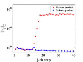
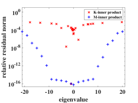
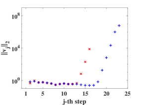
Figure 5.1: Left: the $2$-norms of the Lanczos vectors $v_{j}$. Middle: the relative residual norms of the approximate eigenpairs $(\widehat{\lambda}_{i},\widehat{x}_{i})$. Right: the $2$-norms of the Lanczos vectors $v_{j}$ with (+) and without (x) implicit restart.

For numerical experiments, we take $n=500$ and $m=1$. We use the buckling spectral transformation (1.2) with the shift $\sigma=-0.6$. We run the Lanczos method with $K$-inner product, and the starting vector $Cx_{0}$ with $x_{0}=[1,\ \ldots,\ 1]^{T}$. The approximate eigenpairs $(\widehat{\lambda}_{i},\widehat{x}_{i})$ of (1.1) are computed by $(\widehat{\lambda}_{i},\widehat{x}_{i})=(\frac{\sigma\widehat{\mu}_{i}}{\widehat{\mu}_{i}-1},\widehat{x}_{i})$.

The left plot of Figure 5.1 shows the $2$-norms of 40 Lanczos vectors $v_{j}$. As observed by Meerbergen [20] and Stewart [28], the $2$-norms of Lanczos vectors $v_{j}$ grows rapidly. Consequently, as shown in the middle plot of Figure 5.1, the accuracy of approximate eigenpairs $(\widehat{\lambda}_{i},\widehat{x}_{i})$ deteriorates. In contrast, when we replace the $K$-inner product by the positive definite $M$-inner product with $H_{N}=I_{m}$. We observe that, the $2$-norms of the Lanczos vectors are well bounded. Multiple eigenvalues near the shift $\sigma$ are computed with the relative residual norms around the machine precision.

We note that in [20], Meerbergen proposed to control the norms of the Lanczos vectors by applying implicit restart. We experimented the scheme of implicit restart at $16$-th iteration of the Lanczos method. The results are shown in the right plot of Figure 5.1. We can see that the $2$-norms of the Lanczos vectors with and without implicit restart grows rapidly.

Example 2.

This is an example from the buckling analysis of a finite element model of an airplane shown in Figure 5.2. The size of the pencil $K-\lambda K_{G}$ is $n=67,512$. The stiffness matrix $K$ is positive semi-definite and the dimension of the nullspace $\mathcal{N}(K)$ is known to be $6$, which corresponds to the $6$ rigid body modes [10]. The basis $Z$ of $\mathcal{N}(K)$ is computed by the Gaussian-based method [10]. The dimension of the common nullspace $\mathcal{Z}_{c}$ of $K$ and $K_{G}$ is $3$, which can be easily computed from the basis $Z$, see [13, Theorem 6.4.1]. The accuracy of the bases is shown in the table in Figure 5.2. We are interested in computing the nonzero eigenvalues of the pencil $K-\lambda K_{G}$ in an interval around zero and the associated eigenvectors perpendicular to the common nullspace $\mathcal{Z}_{c}$.

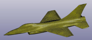
$i$ $d_{i}/\|K_{G}\|_{1}$ $\frac{\|Kz_{i}\|_{2}}{\|K\|_{1}\|z_{i}\|_{2}}$ $\frac{\|K_{G}z_{i}\|_{2}}{\|K_{G}\|_{1}\|z_{i}\|_{2}}$ $1$ $6.90\cdot 10^{-5}$ $2.74\cdot 10^{-16}$ $6.78\cdot 10^{-5}$ $2$ $3.25\cdot 10^{-5}$ $4.88\cdot 10^{-16}$ $9.06\cdot 10^{-6}$ $3$ $2.32\cdot 10^{-5}$ $4.71\cdot 10^{-16}$ $1.19\cdot 10^{-5}$ $4$ $7.32\cdot 10^{-16}$ $2.68\cdot 10^{-17}$ $5.01\cdot 10^{-18}$ $5$ $1.26\cdot 10^{-16}$ $1.90\cdot 10^{-17}$ $4.89\cdot 10^{-18}$ $6$ $7.81\cdot 10^{-18}$ $2.37\cdot 10^{-17}$ $5.00\cdot 10^{-18}$

Figure 5.2: Left: Finite element model of an airplane. Right: Accuracy of the bases for the nullspace of $K$ and common nullspace of $K$ and $K_{G}$, where the second column shows the singular values $d_{i}$ of $K_{G}Y$ with $Y$ being an orthonormal basis of $\mathcal{N}(K)$. The third and fourth columns show the accuracy of the basis $Z=[Z_{N}\ Z_{C}]=[z_{1}\ z_{2}\ \ldots\ z_{6}]$.

We used two methods for computing the matrix-vector product $u=Cv$ described in §3.2. For Method 2, we determine the permutation matrix $P$ by maximizing the number of non-zero entries in the last $n_{3}$ columns of $S$ in (3.24). The MATLAB function ldl, which uses MA57 [6] for real sparse matrices, is used to compute the sparse LDL^T factorization of the augmented matrix $A_{\sigma}$ and the submatrix $S^{\sigma}_{11}$. The pivot tolerance $\tau=0.1$ is used to control the numerical stability of the factorization. In defining the positive definite matrix $M$, we use $H_{N}=\omega D_{N}$ and $H_{C}=\omega I_{n_{3}}$, where $D_{N}$ is a diagonal matrix to normalize each column of the matrix $K_{G}Z_{N}$ and $\omega=\|K\|_{1}$. The starting vector of the Lanczos procedure is $v=Cx_{0}$ with $x_{0}$ being a random vector.

To monitor the progress of the Lanczos method, an approximate eigenpair $(\widehat{\mu}_{i},\widehat{x}_{i})$ computed from an eigenpair $(\widehat{\mu}_{i},\widehat{s}_{i})$ of the reduced matrix $T_{j}$ is considered to have converged if the following two conditions are satisfied:

$$|\widehat{\mu}_{i}|\geq tol\quad\mbox{and}\quad\frac{|\sigma|}{(\widehat{\mu}_{i}-1)^{2}}|\beta_{j}||e_{j}^{T}\widehat{s}_{i}|<tol,$$ (5.1)

where the first condition is used to exclude zero eigenvalues and $tol$ is a prescribed tolerance (see [8, 15] and [24, p. 357]). In this numerical example, we use the tolerance $tol=10^{-6}$.

We now show the numerical results for computing nonzero eigenvalues of the pencil $K-\lambda K_{G}$ and corresponding eigenvectors perpendicular to the common nullspace $\mathcal{Z}_{c}$ in the interval $(-8,8)$. First, let us consider the left-half interval $(-8,0)$. With the shift $\sigma=-4.0$, the shift-invert Lanczos method (Algorithm 1) computed 12 eigenvalues to the machine precision in the interval $(-8,0)$ at $38$-th iteration with either method for the matrix-vector product $u=Cv$. The accuracy of the computed eigenpairs $(\widehat{\lambda}_{i}=\frac{\sigma\widehat{\mu}_{i}}{\widehat{\mu}_{i}-1},\widehat{x}_{i})$ are shown in Table 5.1. To validate the number of eigenvalues in the interval $(-8,0)$, we use the counting scheme described in §4. Using the inertias of the augmented matrix $A_{\alpha}$ with $\alpha=-8$, by Theorem 5, we have

$$n(-8,0)=\nu_{-}(A_{\alpha})-\dim(\mathcal{Z}_{c})-\nu_{-}(Z_{N}^{T}K_{G}Z_{N})=18-3-3=12.$$

This matches the number of eigenvalues found in the interval. Alternatively, by using the inertias of the submatrix $S^{\alpha}_{11}$ with $\alpha=-8$ and Theorem 5, we have

$$n(-8,0)=\nu_{-}(S^{\alpha}_{11})-\nu_{-}(Z_{N}^{T}K_{G}Z_{N})=15-3=12.$$

This also matches the number of computed eigenvalues in the interval.

Table 5.1: Results of 12 computed eigenvalues in the interval $(-8,0)$ after 38 steps of the Lanczos method with the shift $\sigma=-4.0$. For the 3rd and 4th columns, with $\widehat{X}\equiv[\widehat{x}_{1}\ \ldots\ \widehat{x}_{12}]$, $\|\widehat{X}^{T}M\widehat{X}-I_{12}\|_{F}=3.82\cdot 10^{-12}$ and the matrix-vector product $u=Cv$ is computed by Method 1. For the 5th and 6th columns, $\|\widehat{X}^{T}M\widehat{X}-I_{12}\|_{F}=4.55\cdot 10^{-12}$ and the matrix-vector product $u=Cv$ is computed by Method 2.

$i$	$\widehat{\lambda}_{i}$	$\eta(\widehat{\lambda}_{i},\widehat{x}_{i})$	$\cos\angle(\widehat{x}_{i},\mathcal{Z}_{c})$	$\eta(\widehat{\lambda}_{i},\widehat{x}_{i})$	$\cos\angle(\widehat{x}_{i},\mathcal{Z}_{c})$
$1$	$-2.716598$	$1.35\cdot 10^{-17}$	$2.47\cdot 10^{-17}$	$1.47\cdot 10^{-17}$	$1.63\cdot 10^{-17}$
$2$	$-2.883589$	$1.44\cdot 10^{-17}$	$6.32\cdot 10^{-17}$	$2.47\cdot 10^{-17}$	$4.31\cdot 10^{-17}$
$3$	$-3.292700$	$9.49\cdot 10^{-18}$	$5.52\cdot 10^{-17}$	$1.14\cdot 10^{-17}$	$3.66\cdot 10^{-17}$
$4$	$-3.378406$	$1.08\cdot 10^{-17}$	$1.03\cdot 10^{-17}$	$1.20\cdot 10^{-17}$	$3.21\cdot 10^{-17}$
$5$	$-5.754628$	$2.36\cdot 10^{-17}$	$5.81\cdot 10^{-17}$	$2.11\cdot 10^{-17}$	$5.43\cdot 10^{-17}$
$6$	$-5.854071$	$2.19\cdot 10^{-17}$	$1.23\cdot 10^{-16}$	$2.54\cdot 10^{-17}$	$2.36\cdot 10^{-17}$
$7$	$-6.089281$	$6.16\cdot 10^{-17}$	$1.44\cdot 10^{-16}$	$2.17\cdot 10^{-17}$	$2.12\cdot 10^{-17}$
$8$	$-6.228974$	$3.40\cdot 10^{-17}$	$8.58\cdot 10^{-17}$	$2.06\cdot 10^{-17}$	$2.29\cdot 10^{-17}$
$9$	$-6.784766$	$1.91\cdot 10^{-15}$	$7.52\cdot 10^{-17}$	$8.37\cdot 10^{-16}$	$1.67\cdot 10^{-17}$
$10$	$-6.886759$	$5.61\cdot 10^{-15}$	$5.07\cdot 10^{-17}$	$2.88\cdot 10^{-15}$	$5.43\cdot 10^{-17}$
$11$	$-7.561377$	$1.94\cdot 10^{-12}$	$2.70\cdot 10^{-16}$	$1.87\cdot 10^{-12}$	$7.41\cdot 10^{-17}$
$12$	$-7.745144$	$3.87\cdot 10^{-12}$	$1.26\cdot 10^{-16}$	$3.82\cdot 10^{-12}$	$1.28\cdot 10^{-16}$

Next let us consider the right-half interval $(0,8)$. In this case, we use the shift $\sigma=4.0$. By the shift-invert Lanczos method (Algorithm 1), we found 13 eigenvalues to the machine precision in the interval $(0,8)$ at $44$-th iteration with either method for the matrix-vector product $u=Cv$. The accuracy of the computed eigenpairs $(\widehat{\lambda}_{i}=\frac{\sigma\widehat{\mu}_{i}}{\widehat{\mu}_{i}-1},\widehat{x}_{i})$ are shown in Table 5.2. To validate the number of eigenvalues in the interval $(0,8)$, we again use the counting scheme described in §4. Using the inertias of the augmented matrix $A_{\alpha}$ with $\alpha=8$, by Theorem 5, we have

$$n(0,8)=\nu_{-}(A_{\alpha})-\dim(\mathcal{Z}_{c})-\nu_{+}(Z_{N}^{T}K_{G}Z_{N})=16-3-0=13.$$

This matches the number of eigenvalues found in the interval. Alternatively, by using the inertias of the submatrix $S^{\alpha}_{11}$ with $\alpha=8$ and Theorem 5, we have

$$n(0,8)=\nu_{-}(S^{\alpha}_{11})-\nu_{+}(Z_{N}^{T}K_{G}Z_{N})=13-0=13.$$

This also matches the number of computed eigenvalues in the interval.

Table 5.2: Results of 13 computed eigenvalues in the interval $(0,8)$ after 44 steps of the Lanczos method with the shift $\sigma=4.0$. For the 3rd and 4th columns, with $\widehat{X}\equiv[\widehat{x}_{1}\ \ldots\ \widehat{x}_{13}]$, $\|\widehat{X}^{T}M\widehat{X}-I_{13}\|_{F}=1.63\cdot 10^{-11}$ and the matrix-vector product $u=Cv$ is computed by Method 1. For the 5th and 6th columns, $\|\widehat{X}^{T}M\widehat{X}-I_{13}\|_{F}=1.23\cdot 10^{-11}$ and the matrix-vector product $u=Cv$ is computed by Method 2.

$i$	$\widehat{\lambda}_{i}$	$\eta(\widehat{\lambda}_{i},\widehat{x}_{i})$	$\cos\angle(\widehat{x}_{i},\mathcal{Z}_{c})$	$\eta(\widehat{\lambda}_{i},\widehat{x}_{i})$	$\cos\angle(\widehat{x}_{i},\mathcal{Z}_{c})$
$1$	$2.967043$	$1.95\cdot 10^{-17}$	$3.01\cdot 10^{-17}$	$3.88\cdot 10^{-17}$	$3.68\cdot 10^{-17}$
$2$	$3.025965$	$2.64\cdot 10^{-17}$	$2.00\cdot 10^{-16}$	$4.05\cdot 10^{-17}$	$1.46\cdot 10^{-16}$
$3$	$3.917831$	$1.96\cdot 10^{-17}$	$1.84\cdot 10^{-16}$	$1.60\cdot 10^{-17}$	$1.29\cdot 10^{-16}$
$4$	$4.008941$	$2.09\cdot 10^{-17}$	$2.76\cdot 10^{-16}$	$1.60\cdot 10^{-17}$	$1.70\cdot 10^{-16}$
$5$	$4.591063$	$2.31\cdot 10^{-17}$	$3.09\cdot 10^{-16}$	$2.36\cdot 10^{-17}$	$7.40\cdot 10^{-18}$
$6$	$4.662575$	$2.60\cdot 10^{-17}$	$5.19\cdot 10^{-17}$	$2.73\cdot 10^{-17}$	$9.46\cdot 10^{-17}$
$7$	$5.699271$	$4.59\cdot 10^{-17}$	$5.61\cdot 10^{-16}$	$4.15\cdot 10^{-17}$	$6.26\cdot 10^{-17}$
$8$	$5.725937$	$4.70\cdot 10^{-17}$	$7.27\cdot 10^{-17}$	$5.67\cdot 10^{-17}$	$1.16\cdot 10^{-16}$
$9$	$6.465175$	$8.05\cdot 10^{-17}$	$1.08\cdot 10^{-16}$	$6.01\cdot 10^{-16}$	$1.14\cdot 10^{-16}$
$10$	$6.598173$	$1.34\cdot 10^{-15}$	$9.94\cdot 10^{-16}$	$6.85\cdot 10^{-15}$	$3.46\cdot 10^{-16}$
$11$	$7.285975$	$4.39\cdot 10^{-15}$	$3.17\cdot 10^{-15}$	$5.24\cdot 10^{-15}$	$9.52\cdot 10^{-16}$
$12$	$7.626265$	$2.58\cdot 10^{-14}$	$6.71\cdot 10^{-15}$	$2.72\cdot 10^{-14}$	$3.44\cdot 10^{-15}$
$13$	$7.880296$	$1.21\cdot 10^{-12}$	$3.01\cdot 10^{-14}$	$1.26\cdot 10^{-12}$	$2.98\cdot 10^{-14}$

We observed a significant difference in the numbers of the non-zero entries of the triangular factor $L$ in the ldl factorizations of the augmented matrix $A_{\sigma}$ and the submatrix $S_{11}^{\sigma}$. For example, with the shift $\sigma=-4.0$, the number of non-zero entries of $L$ from the submatrix $S_{11}^{\sigma}$ is $15,142,866$, which is $65.5\%$ less than the number of non-zero entries of $L$ from the augmented matrix $A_{\sigma}$, which is $43,940,581$, see Figure 5.3. Similar results are also observed with the shift $\sigma=4.0$. Hence we strongly advocate the use of Method 2 for computing the matrix-vector product $u=Cv$.

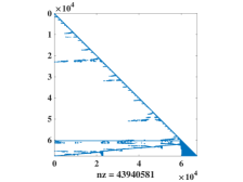
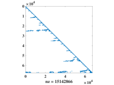
Figure 5.3: The sparsity pattern of the matrices $L$ from the augmented matrix $A_{\sigma}$ (left) and the submatrix $S_{11}^{\sigma}$ (right). The shift is $\sigma=-4.0$ and the pivot tolerance is $\tau=0.1$.

6 Concluding Remark

We studied the buckling eigenvalue problem of singular pencil, and addressed the two open issues associated with the shift-invert Lanczos method. We found that the proposed scheme for counting the number of eigenvalues is a reliable tool for the validation.

Appendix A Canonical form of a symmetric semi-definite pencil $A-\lambda B$

In this section, we give a constructive derivation of a canonical form of a symmetric semi-definite pencil $A-\lambda B$, namely $A$ is symmetric and $B$ is symmetric semi-positive definite.

Theorem 7.

For a symmetric semi-definite pencil $A-\lambda B$, there exists a non-singular matrix $W\in{\mathbb{R}}^{n\times n}$ such that

$$W^{T}AW=\hbox{}\vbox{\kern 0.86108pt\hbox{$\kern 0.0pt\kern 2.5pt\kern-5.0pt\left[\kern 0.0pt\kern-2.5pt\kern-5.55557pt\vbox{\kern-0.86108pt\vbox{\vbox{ \halign{\kern\arraycolsep\hfil\@arstrut$\kbcolstyle#$\hfil\kern\arraycolsep& \kern\arraycolsep\hfil$\@kbrowstyle#$\ifkbalignright\relax\else\hfil\fi\kern\arraycolsep&& \kern\arraycolsep\hfil$\@kbrowstyle#$\ifkbalignright\relax\else\hfil\fi\kern\arraycolsep\cr 5.0pt\hfil\@arstrut$\scriptstyle$\hfil\kern 5.0pt&5.0pt\hfil$\scriptstyle 2n_{0}$\hfil\kern 5.0pt&5.0pt\hfil$\scriptstyle n_{1}$\hfil\kern 5.0pt&5.0pt\hfil$\scriptstyle n_{2}$\hfil\kern 5.0pt&5.0pt\hfil$\scriptstyle n_{3}\\2n_{0}$\hfil\kern 5.0pt&5.0pt\hfil$\scriptstyle S$\hfil\kern 5.0pt&5.0pt\hfil$\scriptstyle$\hfil\kern 5.0pt&5.0pt\hfil$\scriptstyle$\hfil\kern 5.0pt&5.0pt\hfil$\scriptstyle\\n_{1}$\hfil\kern 5.0pt&5.0pt\hfil$\scriptstyle$\hfil\kern 5.0pt&5.0pt\hfil$\scriptstyle\Lambda_{1}$\hfil\kern 5.0pt&5.0pt\hfil$\scriptstyle$\hfil\kern 5.0pt&5.0pt\hfil$\scriptstyle\\n_{2}$\hfil\kern 5.0pt&5.0pt\hfil$\scriptstyle$\hfil\kern 5.0pt&5.0pt\hfil$\scriptstyle$\hfil\kern 5.0pt&5.0pt\hfil$\scriptstyle\Lambda_{2}$\hfil\kern 5.0pt&5.0pt\hfil$\scriptstyle\\n_{3}$\hfil\kern 5.0pt&5.0pt\hfil$\scriptstyle$\hfil\kern 5.0pt&5.0pt\hfil$\scriptstyle$\hfil\kern 5.0pt&5.0pt\hfil$\scriptstyle$\hfil\kern 5.0pt&5.0pt\hfil$\scriptstyle 0$\hfil\kern 5.0pt\crcr}}}}\right]$}}\quad\mbox{and}\quad W^{T}BW=\hbox{}\vbox{\kern 0.86108pt\hbox{$\kern 0.0pt\kern 2.5pt\kern-5.0pt\left[\kern 0.0pt\kern-2.5pt\kern-5.55557pt\vbox{\kern-0.86108pt\vbox{\vbox{ \halign{\kern\arraycolsep\hfil\@arstrut$\kbcolstyle#$\hfil\kern\arraycolsep& \kern\arraycolsep\hfil$\@kbrowstyle#$\ifkbalignright\relax\else\hfil\fi\kern\arraycolsep&& \kern\arraycolsep\hfil$\@kbrowstyle#$\ifkbalignright\relax\else\hfil\fi\kern\arraycolsep\cr 5.0pt\hfil\@arstrut$\scriptstyle$\hfil\kern 5.0pt&5.0pt\hfil$\scriptstyle 2n_{0}$\hfil\kern 5.0pt&5.0pt\hfil$\scriptstyle n_{1}$\hfil\kern 5.0pt&5.0pt\hfil$\scriptstyle n_{2}$\hfil\kern 5.0pt&5.0pt\hfil$\scriptstyle n_{3}\\2n_{0}$\hfil\kern 5.0pt&5.0pt\hfil$\scriptstyle\Omega$\hfil\kern 5.0pt&5.0pt\hfil$\scriptstyle$\hfil\kern 5.0pt&5.0pt\hfil$\scriptstyle$\hfil\kern 5.0pt&5.0pt\hfil$\scriptstyle\\n_{1}$\hfil\kern 5.0pt&5.0pt\hfil$\scriptstyle$\hfil\kern 5.0pt&5.0pt\hfil$\scriptstyle I_{n_{1}}$\hfil\kern 5.0pt&5.0pt\hfil$\scriptstyle$\hfil\kern 5.0pt&5.0pt\hfil$\scriptstyle\\n_{2}$\hfil\kern 5.0pt&5.0pt\hfil$\scriptstyle$\hfil\kern 5.0pt&5.0pt\hfil$\scriptstyle$\hfil\kern 5.0pt&5.0pt\hfil$\scriptstyle 0$\hfil\kern 5.0pt&5.0pt\hfil$\scriptstyle\\n_{3}$\hfil\kern 5.0pt&5.0pt\hfil$\scriptstyle$\hfil\kern 5.0pt&5.0pt\hfil$\scriptstyle$\hfil\kern 5.0pt&5.0pt\hfil$\scriptstyle$\hfil\kern 5.0pt&5.0pt\hfil$\scriptstyle 0$\hfil\kern 5.0pt\crcr}}}}\right]$}},$$ (A.1)

where

$$S\equiv I_{n_{0}}\otimes\left[\begin{array}[]{cc}0&1\\ 1&0\end{array}\right],\quad\Omega\equiv I_{n_{0}}\otimes\left[\begin{array}[]{cc}1&0\\ 0&0\end{array}\right],$$

$\Lambda_{1}$ and $\Lambda_{2}$ are diagonal matrices with real diagonal entries, and $\Lambda_{2}$ is non-singular. Moreover, we have

$$n_{0} =\dim(\mathcal{N}(B))-n_{2}-n_{3},$$

$$n_{1} =\operatorname{rank}(B)-n_{0},$$

$$n_{2} =\operatorname{rank}(\mathcal{P}_{\mathcal{N}(B)}A\mathcal{P}_{\mathcal{N}(B)}),$$

$$n_{3} =\dim(\mathcal{N}(A)\cap\mathcal{N}(B)),$$

where $\mathcal{P}_{\mathcal{N}(B)}$ is the orthogonal projection onto $\mathcal{N}(B)$.

We first introduce the following lemma due to Fix and Heiberger [11], also see [24, Sec. 15.5].

Lemma 5.

For the symmetric semi-definite pencil $A-\lambda B$, there exists a non-singular matrix $W\in{\mathbb{R}}^{n\times n}$ such that

$$W^{T}AW=\hbox{}\vbox{\kern 0.86108pt\hbox{$\kern 0.0pt\kern 2.5pt\kern-5.0pt\left[\kern 0.0pt\kern-2.5pt\kern-5.55557pt\vbox{\kern-0.86108pt\vbox{\vbox{ \halign{\kern\arraycolsep\hfil\@arstrut$\kbcolstyle#$\hfil\kern\arraycolsep& \kern\arraycolsep\hfil$\@kbrowstyle#$\ifkbalignright\relax\else\hfil\fi\kern\arraycolsep&& \kern\arraycolsep\hfil$\@kbrowstyle#$\ifkbalignright\relax\else\hfil\fi\kern\arraycolsep\cr 5.0pt\hfil\@arstrut$\scriptstyle$\hfil\kern 5.0pt&5.0pt\hfil$\scriptstyle n_{0}$\hfil\kern 5.0pt&5.0pt\hfil$\scriptstyle n_{1}$\hfil\kern 5.0pt&5.0pt\hfil$\scriptstyle n_{2}$\hfil\kern 5.0pt&5.0pt\hfil$\scriptstyle n_{0}$\hfil\kern 5.0pt&5.0pt\hfil$\scriptstyle n_{3}\\n_{0}$\hfil\kern 5.0pt&5.0pt\hfil$\scriptstyle A_{00}$\hfil\kern 5.0pt&5.0pt\hfil$\scriptstyle A_{01}$\hfil\kern 5.0pt&5.0pt\hfil$\scriptstyle A_{02}$\hfil\kern 5.0pt&5.0pt\hfil$\scriptstyle\Sigma$\hfil\kern 5.0pt&5.0pt\hfil$\scriptstyle 0\\n_{1}$\hfil\kern 5.0pt&5.0pt\hfil$\scriptstyle A_{01}^{T}$\hfil\kern 5.0pt&5.0pt\hfil$\scriptstyle A_{11}$\hfil\kern 5.0pt&5.0pt\hfil$\scriptstyle A_{12}$\hfil\kern 5.0pt&5.0pt\hfil$\scriptstyle$\hfil\kern 5.0pt&5.0pt\hfil$\scriptstyle\\n_{2}$\hfil\kern 5.0pt&5.0pt\hfil$\scriptstyle A_{02}^{T}$\hfil\kern 5.0pt&5.0pt\hfil$\scriptstyle A_{12}^{T}$\hfil\kern 5.0pt&5.0pt\hfil$\scriptstyle\Lambda_{2}$\hfil\kern 5.0pt&5.0pt\hfil$\scriptstyle$\hfil\kern 5.0pt&5.0pt\hfil$\scriptstyle\\n_{0}$\hfil\kern 5.0pt&5.0pt\hfil$\scriptstyle\Sigma$\hfil\kern 5.0pt&5.0pt\hfil$\scriptstyle$\hfil\kern 5.0pt&5.0pt\hfil$\scriptstyle$\hfil\kern 5.0pt&5.0pt\hfil$\scriptstyle 0$\hfil\kern 5.0pt&5.0pt\hfil$\scriptstyle\\n_{3}$\hfil\kern 5.0pt&5.0pt\hfil$\scriptstyle 0$\hfil\kern 5.0pt&5.0pt\hfil$\scriptstyle$\hfil\kern 5.0pt&5.0pt\hfil$\scriptstyle$\hfil\kern 5.0pt&5.0pt\hfil$\scriptstyle$\hfil\kern 5.0pt&5.0pt\hfil$\scriptstyle 0$\hfil\kern 5.0pt\crcr}}}}\right]$}}\quad\mbox{and}\quad W^{T}BW=\hbox{}\vbox{\kern 0.86108pt\hbox{$\kern 0.0pt\kern 2.5pt\kern-5.0pt\left[\kern 0.0pt\kern-2.5pt\kern-5.55557pt\vbox{\kern-0.86108pt\vbox{\vbox{ \halign{\kern\arraycolsep\hfil\@arstrut$\kbcolstyle#$\hfil\kern\arraycolsep& \kern\arraycolsep\hfil$\@kbrowstyle#$\ifkbalignright\relax\else\hfil\fi\kern\arraycolsep&& \kern\arraycolsep\hfil$\@kbrowstyle#$\ifkbalignright\relax\else\hfil\fi\kern\arraycolsep\cr 5.0pt\hfil\@arstrut$\scriptstyle$\hfil\kern 5.0pt&5.0pt\hfil$\scriptstyle n_{0}$\hfil\kern 5.0pt&5.0pt\hfil$\scriptstyle n_{1}$\hfil\kern 5.0pt&5.0pt\hfil$\scriptstyle n_{2}$\hfil\kern 5.0pt&5.0pt\hfil$\scriptstyle n_{0}$\hfil\kern 5.0pt&5.0pt\hfil$\scriptstyle n_{3}\\n_{0}$\hfil\kern 5.0pt&5.0pt\hfil$\scriptstyle I_{n_{0}}$\hfil\kern 5.0pt&5.0pt\hfil$\scriptstyle$\hfil\kern 5.0pt&5.0pt\hfil$\scriptstyle$\hfil\kern 5.0pt&5.0pt\hfil$\scriptstyle$\hfil\kern 5.0pt&5.0pt\hfil$\scriptstyle\\n_{1}$\hfil\kern 5.0pt&5.0pt\hfil$\scriptstyle$\hfil\kern 5.0pt&5.0pt\hfil$\scriptstyle I_{n_{1}}$\hfil\kern 5.0pt&5.0pt\hfil$\scriptstyle$\hfil\kern 5.0pt&5.0pt\hfil$\scriptstyle$\hfil\kern 5.0pt&5.0pt\hfil$\scriptstyle\\n_{2}$\hfil\kern 5.0pt&5.0pt\hfil$\scriptstyle$\hfil\kern 5.0pt&5.0pt\hfil$\scriptstyle$\hfil\kern 5.0pt&5.0pt\hfil$\scriptstyle 0$\hfil\kern 5.0pt&5.0pt\hfil$\scriptstyle$\hfil\kern 5.0pt&5.0pt\hfil$\scriptstyle\\n_{0}$\hfil\kern 5.0pt&5.0pt\hfil$\scriptstyle$\hfil\kern 5.0pt&5.0pt\hfil$\scriptstyle$\hfil\kern 5.0pt&5.0pt\hfil$\scriptstyle$\hfil\kern 5.0pt&5.0pt\hfil$\scriptstyle 0$\hfil\kern 5.0pt&5.0pt\hfil$\scriptstyle\\n_{3}$\hfil\kern 5.0pt&5.0pt\hfil$\scriptstyle$\hfil\kern 5.0pt&5.0pt\hfil$\scriptstyle$\hfil\kern 5.0pt&5.0pt\hfil$\scriptstyle$\hfil\kern 5.0pt&5.0pt\hfil$\scriptstyle$\hfil\kern 5.0pt&5.0pt\hfil$\scriptstyle 0$\hfil\kern 5.0pt\crcr}}}}\right]$}},$$

where $\Lambda_{2}$ and $\Sigma$ are non-singular, diagonal matrices with real diagonal entries.

Proof of Theorem 7. By Lemma 5, there exists a non-singular matrix $W_{0}\in{\mathbb{R}}^{n\times n}$ such that

$$A^{(1)}\equiv W_{0}^{T}AW_{0}=\hbox{}\vbox{\kern 0.86108pt\hbox{$\kern 0.0pt\kern 2.5pt\kern-5.0pt\left[\kern 0.0pt\kern-2.5pt\kern-5.55557pt\vbox{\kern-0.86108pt\vbox{\vbox{ \halign{\kern\arraycolsep\hfil\@arstrut$\kbcolstyle#$\hfil\kern\arraycolsep& \kern\arraycolsep\hfil$\@kbrowstyle#$\ifkbalignright\relax\else\hfil\fi\kern\arraycolsep&& \kern\arraycolsep\hfil$\@kbrowstyle#$\ifkbalignright\relax\else\hfil\fi\kern\arraycolsep\cr 5.0pt\hfil\@arstrut$\scriptstyle$\hfil\kern 5.0pt&5.0pt\hfil$\scriptstyle n_{0}$\hfil\kern 5.0pt&5.0pt\hfil$\scriptstyle n_{1}$\hfil\kern 5.0pt&5.0pt\hfil$\scriptstyle n_{2}$\hfil\kern 5.0pt&5.0pt\hfil$\scriptstyle n_{0}$\hfil\kern 5.0pt&5.0pt\hfil$\scriptstyle n_{3}\\n_{0}$\hfil\kern 5.0pt&5.0pt\hfil$\scriptstyle A_{00}$\hfil\kern 5.0pt&5.0pt\hfil$\scriptstyle A_{01}$\hfil\kern 5.0pt&5.0pt\hfil$\scriptstyle A_{02}$\hfil\kern 5.0pt&5.0pt\hfil$\scriptstyle\Sigma$\hfil\kern 5.0pt&5.0pt\hfil$\scriptstyle 0\\n_{1}$\hfil\kern 5.0pt&5.0pt\hfil$\scriptstyle A_{01}^{T}$\hfil\kern 5.0pt&5.0pt\hfil$\scriptstyle A_{11}$\hfil\kern 5.0pt&5.0pt\hfil$\scriptstyle A_{12}$\hfil\kern 5.0pt&5.0pt\hfil$\scriptstyle$\hfil\kern 5.0pt&5.0pt\hfil$\scriptstyle\\n_{2}$\hfil\kern 5.0pt&5.0pt\hfil$\scriptstyle A_{02}^{T}$\hfil\kern 5.0pt&5.0pt\hfil$\scriptstyle A_{12}^{T}$\hfil\kern 5.0pt&5.0pt\hfil$\scriptstyle\Lambda_{2}$\hfil\kern 5.0pt&5.0pt\hfil$\scriptstyle$\hfil\kern 5.0pt&5.0pt\hfil$\scriptstyle\\n_{0}$\hfil\kern 5.0pt&5.0pt\hfil$\scriptstyle\Sigma$\hfil\kern 5.0pt&5.0pt\hfil$\scriptstyle$\hfil\kern 5.0pt&5.0pt\hfil$\scriptstyle$\hfil\kern 5.0pt&5.0pt\hfil$\scriptstyle 0$\hfil\kern 5.0pt&5.0pt\hfil$\scriptstyle\\n_{3}$\hfil\kern 5.0pt&5.0pt\hfil$\scriptstyle 0$\hfil\kern 5.0pt&5.0pt\hfil$\scriptstyle$\hfil\kern 5.0pt&5.0pt\hfil$\scriptstyle$\hfil\kern 5.0pt&5.0pt\hfil$\scriptstyle$\hfil\kern 5.0pt&5.0pt\hfil$\scriptstyle 0$\hfil\kern 5.0pt\crcr}}}}\right]$}}\quad\mbox{and}\quad B^{(1)}\equiv W_{0}^{T}BW_{0}=\hbox{}\vbox{\kern 0.86108pt\hbox{$\kern 0.0pt\kern 2.5pt\kern-5.0pt\left[\kern 0.0pt\kern-2.5pt\kern-5.55557pt\vbox{\kern-0.86108pt\vbox{\vbox{ \halign{\kern\arraycolsep\hfil\@arstrut$\kbcolstyle#$\hfil\kern\arraycolsep& \kern\arraycolsep\hfil$\@kbrowstyle#$\ifkbalignright\relax\else\hfil\fi\kern\arraycolsep&& \kern\arraycolsep\hfil$\@kbrowstyle#$\ifkbalignright\relax\else\hfil\fi\kern\arraycolsep\cr 5.0pt\hfil\@arstrut$\scriptstyle$\hfil\kern 5.0pt&5.0pt\hfil$\scriptstyle n_{0}$\hfil\kern 5.0pt&5.0pt\hfil$\scriptstyle n_{1}$\hfil\kern 5.0pt&5.0pt\hfil$\scriptstyle n_{2}$\hfil\kern 5.0pt&5.0pt\hfil$\scriptstyle n_{0}$\hfil\kern 5.0pt&5.0pt\hfil$\scriptstyle n_{3}\\n_{0}$\hfil\kern 5.0pt&5.0pt\hfil$\scriptstyle I_{n_{0}}$\hfil\kern 5.0pt&5.0pt\hfil$\scriptstyle$\hfil\kern 5.0pt&5.0pt\hfil$\scriptstyle$\hfil\kern 5.0pt&5.0pt\hfil$\scriptstyle$\hfil\kern 5.0pt&5.0pt\hfil$\scriptstyle\\n_{1}$\hfil\kern 5.0pt&5.0pt\hfil$\scriptstyle$\hfil\kern 5.0pt&5.0pt\hfil$\scriptstyle I_{n_{1}}$\hfil\kern 5.0pt&5.0pt\hfil$\scriptstyle$\hfil\kern 5.0pt&5.0pt\hfil$\scriptstyle$\hfil\kern 5.0pt&5.0pt\hfil$\scriptstyle\\n_{2}$\hfil\kern 5.0pt&5.0pt\hfil$\scriptstyle$\hfil\kern 5.0pt&5.0pt\hfil$\scriptstyle$\hfil\kern 5.0pt&5.0pt\hfil$\scriptstyle 0$\hfil\kern 5.0pt&5.0pt\hfil$\scriptstyle$\hfil\kern 5.0pt&5.0pt\hfil$\scriptstyle\\n_{0}$\hfil\kern 5.0pt&5.0pt\hfil$\scriptstyle$\hfil\kern 5.0pt&5.0pt\hfil$\scriptstyle$\hfil\kern 5.0pt&5.0pt\hfil$\scriptstyle$\hfil\kern 5.0pt&5.0pt\hfil$\scriptstyle 0$\hfil\kern 5.0pt&5.0pt\hfil$\scriptstyle\\n_{3}$\hfil\kern 5.0pt&5.0pt\hfil$\scriptstyle$\hfil\kern 5.0pt&5.0pt\hfil$\scriptstyle$\hfil\kern 5.0pt&5.0pt\hfil$\scriptstyle$\hfil\kern 5.0pt&5.0pt\hfil$\scriptstyle$\hfil\kern 5.0pt&5.0pt\hfil$\scriptstyle 0$\hfil\kern 5.0pt\crcr}}}}\right]$}},$$

where $\Lambda_{2}$ and $\Sigma$ are non-singular, diagonal matrices with real diagonal entries.

Let

$$W_{1}\equiv\hbox{}\vbox{\kern 0.86108pt\hbox{$\kern 0.0pt\kern 2.5pt\kern-5.0pt\left[\kern 0.0pt\kern-2.5pt\kern-5.55557pt\vbox{\kern-0.86108pt\vbox{\vbox{ \halign{\kern\arraycolsep\hfil\@arstrut$\kbcolstyle#$\hfil\kern\arraycolsep& \kern\arraycolsep\hfil$\@kbrowstyle#$\ifkbalignright\relax\else\hfil\fi\kern\arraycolsep&& \kern\arraycolsep\hfil$\@kbrowstyle#$\ifkbalignright\relax\else\hfil\fi\kern\arraycolsep\cr 5.0pt\hfil\@arstrut$\scriptstyle$\hfil\kern 5.0pt&5.0pt\hfil$\scriptstyle n_{0}$\hfil\kern 5.0pt&5.0pt\hfil$\scriptstyle n_{1}$\hfil\kern 5.0pt&5.0pt\hfil$\scriptstyle n_{2}$\hfil\kern 5.0pt&5.0pt\hfil$\scriptstyle n_{0}$\hfil\kern 5.0pt&5.0pt\hfil$\scriptstyle n_{3}\\n_{0}$\hfil\kern 5.0pt&5.0pt\hfil$\scriptstyle I_{n_{0}}$\hfil\kern 5.0pt&5.0pt\hfil$\scriptstyle$\hfil\kern 5.0pt&5.0pt\hfil$\scriptstyle$\hfil\kern 5.0pt&5.0pt\hfil$\scriptstyle$\hfil\kern 5.0pt&5.0pt\hfil$\scriptstyle\\n_{1}$\hfil\kern 5.0pt&5.0pt\hfil$\scriptstyle$\hfil\kern 5.0pt&5.0pt\hfil$\scriptstyle I_{n_{1}}$\hfil\kern 5.0pt&5.0pt\hfil$\scriptstyle$\hfil\kern 5.0pt&5.0pt\hfil$\scriptstyle$\hfil\kern 5.0pt&5.0pt\hfil$\scriptstyle\\n_{2}$\hfil\kern 5.0pt&5.0pt\hfil$\scriptstyle$\hfil\kern 5.0pt&5.0pt\hfil$\scriptstyle$\hfil\kern 5.0pt&5.0pt\hfil$\scriptstyle I_{n_{2}}$\hfil\kern 5.0pt&5.0pt\hfil$\scriptstyle$\hfil\kern 5.0pt&5.0pt\hfil$\scriptstyle\\n_{0}$\hfil\kern 5.0pt&5.0pt\hfil$\scriptstyle-\Sigma^{-1}A_{00}/2$\hfil\kern 5.0pt&5.0pt\hfil$\scriptstyle-\Sigma^{-1}A_{01}$\hfil\kern 5.0pt&5.0pt\hfil$\scriptstyle-\Sigma^{-1}A_{02}$\hfil\kern 5.0pt&5.0pt\hfil$\scriptstyle I_{n_{0}}$\hfil\kern 5.0pt&5.0pt\hfil$\scriptstyle\\n_{3}$\hfil\kern 5.0pt&5.0pt\hfil$\scriptstyle$\hfil\kern 5.0pt&5.0pt\hfil$\scriptstyle$\hfil\kern 5.0pt&5.0pt\hfil$\scriptstyle$\hfil\kern 5.0pt&5.0pt\hfil$\scriptstyle$\hfil\kern 5.0pt&5.0pt\hfil$\scriptstyle I_{n_{3}}$\hfil\kern 5.0pt\crcr}}}}\right]$}},$$

then

$$A^{(2)}\equiv W_{1}^{T}A^{(1)}W_{1}=\hbox{}\vbox{\kern 0.86108pt\hbox{$\kern 0.0pt\kern 2.5pt\kern-5.0pt\left[\kern 0.0pt\kern-2.5pt\kern-5.55557pt\vbox{\kern-0.86108pt\vbox{\vbox{ \halign{\kern\arraycolsep\hfil\@arstrut$\kbcolstyle#$\hfil\kern\arraycolsep& \kern\arraycolsep\hfil$\@kbrowstyle#$\ifkbalignright\relax\else\hfil\fi\kern\arraycolsep&& \kern\arraycolsep\hfil$\@kbrowstyle#$\ifkbalignright\relax\else\hfil\fi\kern\arraycolsep\cr 5.0pt\hfil\@arstrut$\scriptstyle$\hfil\kern 5.0pt&5.0pt\hfil$\scriptstyle n_{0}$\hfil\kern 5.0pt&5.0pt\hfil$\scriptstyle n_{1}$\hfil\kern 5.0pt&5.0pt\hfil$\scriptstyle n_{2}$\hfil\kern 5.0pt&5.0pt\hfil$\scriptstyle n_{0}$\hfil\kern 5.0pt&5.0pt\hfil$\scriptstyle n_{3}\\n_{0}$\hfil\kern 5.0pt&5.0pt\hfil$\scriptstyle 0$\hfil\kern 5.0pt&5.0pt\hfil$\scriptstyle$\hfil\kern 5.0pt&5.0pt\hfil$\scriptstyle$\hfil\kern 5.0pt&5.0pt\hfil$\scriptstyle\Sigma$\hfil\kern 5.0pt&5.0pt\hfil$\scriptstyle\\n_{1}$\hfil\kern 5.0pt&5.0pt\hfil$\scriptstyle$\hfil\kern 5.0pt&5.0pt\hfil$\scriptstyle A_{11}$\hfil\kern 5.0pt&5.0pt\hfil$\scriptstyle A_{12}$\hfil\kern 5.0pt&5.0pt\hfil$\scriptstyle$\hfil\kern 5.0pt&5.0pt\hfil$\scriptstyle\\n_{2}$\hfil\kern 5.0pt&5.0pt\hfil$\scriptstyle$\hfil\kern 5.0pt&5.0pt\hfil$\scriptstyle A_{12}^{T}$\hfil\kern 5.0pt&5.0pt\hfil$\scriptstyle\Lambda_{2}$\hfil\kern 5.0pt&5.0pt\hfil$\scriptstyle$\hfil\kern 5.0pt&5.0pt\hfil$\scriptstyle\\n_{0}$\hfil\kern 5.0pt&5.0pt\hfil$\scriptstyle\Sigma$\hfil\kern 5.0pt&5.0pt\hfil$\scriptstyle$\hfil\kern 5.0pt&5.0pt\hfil$\scriptstyle$\hfil\kern 5.0pt&5.0pt\hfil$\scriptstyle 0$\hfil\kern 5.0pt&5.0pt\hfil$\scriptstyle\\n_{3}$\hfil\kern 5.0pt&5.0pt\hfil$\scriptstyle$\hfil\kern 5.0pt&5.0pt\hfil$\scriptstyle$\hfil\kern 5.0pt&5.0pt\hfil$\scriptstyle$\hfil\kern 5.0pt&5.0pt\hfil$\scriptstyle$\hfil\kern 5.0pt&5.0pt\hfil$\scriptstyle 0$\hfil\kern 5.0pt\crcr}}}}\right]$}}\quad\mbox{and}\quad B^{(2)}\equiv W_{1}^{T}B^{(1)}W_{1}=\hbox{}\vbox{\kern 0.86108pt\hbox{$\kern 0.0pt\kern 2.5pt\kern-5.0pt\left[\kern 0.0pt\kern-2.5pt\kern-5.55557pt\vbox{\kern-0.86108pt\vbox{\vbox{ \halign{\kern\arraycolsep\hfil\@arstrut$\kbcolstyle#$\hfil\kern\arraycolsep& \kern\arraycolsep\hfil$\@kbrowstyle#$\ifkbalignright\relax\else\hfil\fi\kern\arraycolsep&& \kern\arraycolsep\hfil$\@kbrowstyle#$\ifkbalignright\relax\else\hfil\fi\kern\arraycolsep\cr 5.0pt\hfil\@arstrut$\scriptstyle$\hfil\kern 5.0pt&5.0pt\hfil$\scriptstyle n_{0}$\hfil\kern 5.0pt&5.0pt\hfil$\scriptstyle n_{1}$\hfil\kern 5.0pt&5.0pt\hfil$\scriptstyle n_{2}$\hfil\kern 5.0pt&5.0pt\hfil$\scriptstyle n_{0}$\hfil\kern 5.0pt&5.0pt\hfil$\scriptstyle n_{3}\\n_{0}$\hfil\kern 5.0pt&5.0pt\hfil$\scriptstyle I_{n_{0}}$\hfil\kern 5.0pt&5.0pt\hfil$\scriptstyle$\hfil\kern 5.0pt&5.0pt\hfil$\scriptstyle$\hfil\kern 5.0pt&5.0pt\hfil$\scriptstyle$\hfil\kern 5.0pt&5.0pt\hfil$\scriptstyle\\n_{1}$\hfil\kern 5.0pt&5.0pt\hfil$\scriptstyle$\hfil\kern 5.0pt&5.0pt\hfil$\scriptstyle I_{n_{1}}$\hfil\kern 5.0pt&5.0pt\hfil$\scriptstyle$\hfil\kern 5.0pt&5.0pt\hfil$\scriptstyle$\hfil\kern 5.0pt&5.0pt\hfil$\scriptstyle\\n_{2}$\hfil\kern 5.0pt&5.0pt\hfil$\scriptstyle$\hfil\kern 5.0pt&5.0pt\hfil$\scriptstyle$\hfil\kern 5.0pt&5.0pt\hfil$\scriptstyle 0$\hfil\kern 5.0pt&5.0pt\hfil$\scriptstyle$\hfil\kern 5.0pt&5.0pt\hfil$\scriptstyle\\n_{0}$\hfil\kern 5.0pt&5.0pt\hfil$\scriptstyle$\hfil\kern 5.0pt&5.0pt\hfil$\scriptstyle$\hfil\kern 5.0pt&5.0pt\hfil$\scriptstyle$\hfil\kern 5.0pt&5.0pt\hfil$\scriptstyle 0$\hfil\kern 5.0pt&5.0pt\hfil$\scriptstyle\\n_{3}$\hfil\kern 5.0pt&5.0pt\hfil$\scriptstyle$\hfil\kern 5.0pt&5.0pt\hfil$\scriptstyle$\hfil\kern 5.0pt&5.0pt\hfil$\scriptstyle$\hfil\kern 5.0pt&5.0pt\hfil$\scriptstyle$\hfil\kern 5.0pt&5.0pt\hfil$\scriptstyle 0$\hfil\kern 5.0pt\crcr}}}}\right]$}}.$$

Next let

$$W_{2}\equiv\hbox{}\vbox{\kern 0.86108pt\hbox{$\kern 0.0pt\kern 2.5pt\kern-5.0pt\left[\kern 0.0pt\kern-2.5pt\kern-5.55557pt\vbox{\kern-0.86108pt\vbox{\vbox{ \halign{\kern\arraycolsep\hfil\@arstrut$\kbcolstyle#$\hfil\kern\arraycolsep& \kern\arraycolsep\hfil$\@kbrowstyle#$\ifkbalignright\relax\else\hfil\fi\kern\arraycolsep&& \kern\arraycolsep\hfil$\@kbrowstyle#$\ifkbalignright\relax\else\hfil\fi\kern\arraycolsep\cr 5.0pt\hfil\@arstrut$\scriptstyle$\hfil\kern 5.0pt&5.0pt\hfil$\scriptstyle n_{0}$\hfil\kern 5.0pt&5.0pt\hfil$\scriptstyle n_{1}$\hfil\kern 5.0pt&5.0pt\hfil$\scriptstyle n_{2}$\hfil\kern 5.0pt&5.0pt\hfil$\scriptstyle n_{0}$\hfil\kern 5.0pt&5.0pt\hfil$\scriptstyle n_{3}\\n_{0}$\hfil\kern 5.0pt&5.0pt\hfil$\scriptstyle I_{n_{0}}$\hfil\kern 5.0pt&5.0pt\hfil$\scriptstyle$\hfil\kern 5.0pt&5.0pt\hfil$\scriptstyle$\hfil\kern 5.0pt&5.0pt\hfil$\scriptstyle$\hfil\kern 5.0pt&5.0pt\hfil$\scriptstyle\\n_{1}$\hfil\kern 5.0pt&5.0pt\hfil$\scriptstyle$\hfil\kern 5.0pt&5.0pt\hfil$\scriptstyle I_{n_{1}}$\hfil\kern 5.0pt&5.0pt\hfil$\scriptstyle$\hfil\kern 5.0pt&5.0pt\hfil$\scriptstyle$\hfil\kern 5.0pt&5.0pt\hfil$\scriptstyle\\n_{2}$\hfil\kern 5.0pt&5.0pt\hfil$\scriptstyle$\hfil\kern 5.0pt&5.0pt\hfil$\scriptstyle-\Lambda_{2}^{-1}A_{12}^{T}$\hfil\kern 5.0pt&5.0pt\hfil$\scriptstyle I_{n_{2}}$\hfil\kern 5.0pt&5.0pt\hfil$\scriptstyle$\hfil\kern 5.0pt&5.0pt\hfil$\scriptstyle\\n_{0}$\hfil\kern 5.0pt&5.0pt\hfil$\scriptstyle$\hfil\kern 5.0pt&5.0pt\hfil$\scriptstyle$\hfil\kern 5.0pt&5.0pt\hfil$\scriptstyle$\hfil\kern 5.0pt&5.0pt\hfil$\scriptstyle I_{n_{0}}$\hfil\kern 5.0pt&5.0pt\hfil$\scriptstyle\\n_{3}$\hfil\kern 5.0pt&5.0pt\hfil$\scriptstyle$\hfil\kern 5.0pt&5.0pt\hfil$\scriptstyle$\hfil\kern 5.0pt&5.0pt\hfil$\scriptstyle$\hfil\kern 5.0pt&5.0pt\hfil$\scriptstyle$\hfil\kern 5.0pt&5.0pt\hfil$\scriptstyle I_{n_{3}}$\hfil\kern 5.0pt\crcr}}}}\right]$}},$$

then

$$A^{(3)}\equiv W_{2}^{T}A^{(2)}W_{2}=\hbox{}\vbox{\kern 0.86108pt\hbox{$\kern 0.0pt\kern 2.5pt\kern-5.0pt\left[\kern 0.0pt\kern-2.5pt\kern-5.55557pt\vbox{\kern-0.86108pt\vbox{\vbox{ \halign{\kern\arraycolsep\hfil\@arstrut$\kbcolstyle#$\hfil\kern\arraycolsep& \kern\arraycolsep\hfil$\@kbrowstyle#$\ifkbalignright\relax\else\hfil\fi\kern\arraycolsep&& \kern\arraycolsep\hfil$\@kbrowstyle#$\ifkbalignright\relax\else\hfil\fi\kern\arraycolsep\cr 5.0pt\hfil\@arstrut$\scriptstyle$\hfil\kern 5.0pt&5.0pt\hfil$\scriptstyle n_{0}$\hfil\kern 5.0pt&5.0pt\hfil$\scriptstyle n_{1}$\hfil\kern 5.0pt&5.0pt\hfil$\scriptstyle n_{2}$\hfil\kern 5.0pt&5.0pt\hfil$\scriptstyle n_{0}$\hfil\kern 5.0pt&5.0pt\hfil$\scriptstyle n_{3}\\n_{0}$\hfil\kern 5.0pt&5.0pt\hfil$\scriptstyle 0$\hfil\kern 5.0pt&5.0pt\hfil$\scriptstyle$\hfil\kern 5.0pt&5.0pt\hfil$\scriptstyle$\hfil\kern 5.0pt&5.0pt\hfil$\scriptstyle\Sigma$\hfil\kern 5.0pt&5.0pt\hfil$\scriptstyle\\n_{1}$\hfil\kern 5.0pt&5.0pt\hfil$\scriptstyle$\hfil\kern 5.0pt&5.0pt\hfil$\scriptstyle C_{11}$\hfil\kern 5.0pt&5.0pt\hfil$\scriptstyle$\hfil\kern 5.0pt&5.0pt\hfil$\scriptstyle$\hfil\kern 5.0pt&5.0pt\hfil$\scriptstyle\\n_{2}$\hfil\kern 5.0pt&5.0pt\hfil$\scriptstyle$\hfil\kern 5.0pt&5.0pt\hfil$\scriptstyle$\hfil\kern 5.0pt&5.0pt\hfil$\scriptstyle\Lambda_{2}$\hfil\kern 5.0pt&5.0pt\hfil$\scriptstyle$\hfil\kern 5.0pt&5.0pt\hfil$\scriptstyle\\n_{0}$\hfil\kern 5.0pt&5.0pt\hfil$\scriptstyle\Sigma$\hfil\kern 5.0pt&5.0pt\hfil$\scriptstyle$\hfil\kern 5.0pt&5.0pt\hfil$\scriptstyle$\hfil\kern 5.0pt&5.0pt\hfil$\scriptstyle 0$\hfil\kern 5.0pt&5.0pt\hfil$\scriptstyle\\n_{3}$\hfil\kern 5.0pt&5.0pt\hfil$\scriptstyle$\hfil\kern 5.0pt&5.0pt\hfil$\scriptstyle$\hfil\kern 5.0pt&5.0pt\hfil$\scriptstyle$\hfil\kern 5.0pt&5.0pt\hfil$\scriptstyle$\hfil\kern 5.0pt&5.0pt\hfil$\scriptstyle 0$\hfil\kern 5.0pt\crcr}}}}\right]$}}\quad\mbox{and}\quad B^{(3)}\equiv W_{2}^{T}B^{(2)}W_{2}=\hbox{}\vbox{\kern 0.86108pt\hbox{$\kern 0.0pt\kern 2.5pt\kern-5.0pt\left[\kern 0.0pt\kern-2.5pt\kern-5.55557pt\vbox{\kern-0.86108pt\vbox{\vbox{ \halign{\kern\arraycolsep\hfil\@arstrut$\kbcolstyle#$\hfil\kern\arraycolsep& \kern\arraycolsep\hfil$\@kbrowstyle#$\ifkbalignright\relax\else\hfil\fi\kern\arraycolsep&& \kern\arraycolsep\hfil$\@kbrowstyle#$\ifkbalignright\relax\else\hfil\fi\kern\arraycolsep\cr 5.0pt\hfil\@arstrut$\scriptstyle$\hfil\kern 5.0pt&5.0pt\hfil$\scriptstyle n_{0}$\hfil\kern 5.0pt&5.0pt\hfil$\scriptstyle n_{1}$\hfil\kern 5.0pt&5.0pt\hfil$\scriptstyle n_{2}$\hfil\kern 5.0pt&5.0pt\hfil$\scriptstyle n_{0}$\hfil\kern 5.0pt&5.0pt\hfil$\scriptstyle n_{3}\\n_{0}$\hfil\kern 5.0pt&5.0pt\hfil$\scriptstyle I_{n_{0}}$\hfil\kern 5.0pt&5.0pt\hfil$\scriptstyle$\hfil\kern 5.0pt&5.0pt\hfil$\scriptstyle$\hfil\kern 5.0pt&5.0pt\hfil$\scriptstyle$\hfil\kern 5.0pt&5.0pt\hfil$\scriptstyle\\n_{1}$\hfil\kern 5.0pt&5.0pt\hfil$\scriptstyle$\hfil\kern 5.0pt&5.0pt\hfil$\scriptstyle I_{n_{1}}$\hfil\kern 5.0pt&5.0pt\hfil$\scriptstyle$\hfil\kern 5.0pt&5.0pt\hfil$\scriptstyle$\hfil\kern 5.0pt&5.0pt\hfil$\scriptstyle\\n_{2}$\hfil\kern 5.0pt&5.0pt\hfil$\scriptstyle$\hfil\kern 5.0pt&5.0pt\hfil$\scriptstyle$\hfil\kern 5.0pt&5.0pt\hfil$\scriptstyle 0$\hfil\kern 5.0pt&5.0pt\hfil$\scriptstyle$\hfil\kern 5.0pt&5.0pt\hfil$\scriptstyle\\n_{0}$\hfil\kern 5.0pt&5.0pt\hfil$\scriptstyle$\hfil\kern 5.0pt&5.0pt\hfil$\scriptstyle$\hfil\kern 5.0pt&5.0pt\hfil$\scriptstyle$\hfil\kern 5.0pt&5.0pt\hfil$\scriptstyle 0$\hfil\kern 5.0pt&5.0pt\hfil$\scriptstyle\\n_{3}$\hfil\kern 5.0pt&5.0pt\hfil$\scriptstyle$\hfil\kern 5.0pt&5.0pt\hfil$\scriptstyle$\hfil\kern 5.0pt&5.0pt\hfil$\scriptstyle$\hfil\kern 5.0pt&5.0pt\hfil$\scriptstyle$\hfil\kern 5.0pt&5.0pt\hfil$\scriptstyle 0$\hfil\kern 5.0pt\crcr}}}}\right]$}},$$

where $C_{11}\in{\mathbb{R}}^{n_{1}\times n_{1}}$ is symmetric and $C_{11}=A_{11}-A_{12}\Lambda_{2}^{-1}A_{12}^{T}$.

Define the permutation matrix

$$P_{3}\equiv\left[\begin{array}[]{ccccc}I_{n_{0}}&0&0&0&0\\ 0&0&I_{n_{1}}&0&0\\ 0&0&0&I_{n_{2}}&0\\ 0&I_{n_{0}}&0&0&0\\ 0&0&0&0&I_{n_{3}}\end{array}\right],$$

then

$$A^{(4)}\equiv P_{3}^{T}A^{(3)}P_{3}=\hbox{}\vbox{\kern 0.86108pt\hbox{$\kern 0.0pt\kern 2.5pt\kern-5.0pt\left[\kern 0.0pt\kern-2.5pt\kern-5.55557pt\vbox{\kern-0.86108pt\vbox{\vbox{ \halign{\kern\arraycolsep\hfil\@arstrut$\kbcolstyle#$\hfil\kern\arraycolsep& \kern\arraycolsep\hfil$\@kbrowstyle#$\ifkbalignright\relax\else\hfil\fi\kern\arraycolsep&& \kern\arraycolsep\hfil$\@kbrowstyle#$\ifkbalignright\relax\else\hfil\fi\kern\arraycolsep\cr 5.0pt\hfil\@arstrut$\scriptstyle$\hfil\kern 5.0pt&5.0pt\hfil$\scriptstyle n_{0}$\hfil\kern 5.0pt&5.0pt\hfil$\scriptstyle n_{0}$\hfil\kern 5.0pt&5.0pt\hfil$\scriptstyle n_{1}$\hfil\kern 5.0pt&5.0pt\hfil$\scriptstyle n_{2}$\hfil\kern 5.0pt&5.0pt\hfil$\scriptstyle n_{3}\\n_{0}$\hfil\kern 5.0pt&5.0pt\hfil$\scriptstyle$\hfil\kern 5.0pt&5.0pt\hfil$\scriptstyle\Sigma$\hfil\kern 5.0pt&5.0pt\hfil$\scriptstyle$\hfil\kern 5.0pt&5.0pt\hfil$\scriptstyle$\hfil\kern 5.0pt&5.0pt\hfil$\scriptstyle\\n_{0}$\hfil\kern 5.0pt&5.0pt\hfil$\scriptstyle\Sigma$\hfil\kern 5.0pt&5.0pt\hfil$\scriptstyle$\hfil\kern 5.0pt&5.0pt\hfil$\scriptstyle$\hfil\kern 5.0pt&5.0pt\hfil$\scriptstyle$\hfil\kern 5.0pt&5.0pt\hfil$\scriptstyle\\n_{1}$\hfil\kern 5.0pt&5.0pt\hfil$\scriptstyle$\hfil\kern 5.0pt&5.0pt\hfil$\scriptstyle$\hfil\kern 5.0pt&5.0pt\hfil$\scriptstyle C_{11}$\hfil\kern 5.0pt&5.0pt\hfil$\scriptstyle$\hfil\kern 5.0pt&5.0pt\hfil$\scriptstyle\\n_{2}$\hfil\kern 5.0pt&5.0pt\hfil$\scriptstyle$\hfil\kern 5.0pt&5.0pt\hfil$\scriptstyle$\hfil\kern 5.0pt&5.0pt\hfil$\scriptstyle$\hfil\kern 5.0pt&5.0pt\hfil$\scriptstyle\Lambda_{2}$\hfil\kern 5.0pt&5.0pt\hfil$\scriptstyle\\n_{3}$\hfil\kern 5.0pt&5.0pt\hfil$\scriptstyle$\hfil\kern 5.0pt&5.0pt\hfil$\scriptstyle$\hfil\kern 5.0pt&5.0pt\hfil$\scriptstyle$\hfil\kern 5.0pt&5.0pt\hfil$\scriptstyle$\hfil\kern 5.0pt&5.0pt\hfil$\scriptstyle 0$\hfil\kern 5.0pt\crcr}}}}\right]$}}\quad\mbox{and}\quad B^{(4)}\equiv P_{3}^{T}B^{(3)}P_{3}=\hbox{}\vbox{\kern 0.86108pt\hbox{$\kern 0.0pt\kern 2.5pt\kern-5.0pt\left[\kern 0.0pt\kern-2.5pt\kern-5.55557pt\vbox{\kern-0.86108pt\vbox{\vbox{ \halign{\kern\arraycolsep\hfil\@arstrut$\kbcolstyle#$\hfil\kern\arraycolsep& \kern\arraycolsep\hfil$\@kbrowstyle#$\ifkbalignright\relax\else\hfil\fi\kern\arraycolsep&& \kern\arraycolsep\hfil$\@kbrowstyle#$\ifkbalignright\relax\else\hfil\fi\kern\arraycolsep\cr 5.0pt\hfil\@arstrut$\scriptstyle$\hfil\kern 5.0pt&5.0pt\hfil$\scriptstyle n_{0}$\hfil\kern 5.0pt&5.0pt\hfil$\scriptstyle n_{0}$\hfil\kern 5.0pt&5.0pt\hfil$\scriptstyle n_{1}$\hfil\kern 5.0pt&5.0pt\hfil$\scriptstyle n_{2}$\hfil\kern 5.0pt&5.0pt\hfil$\scriptstyle n_{3}\\n_{0}$\hfil\kern 5.0pt&5.0pt\hfil$\scriptstyle I_{n_{0}}$\hfil\kern 5.0pt&5.0pt\hfil$\scriptstyle$\hfil\kern 5.0pt&5.0pt\hfil$\scriptstyle$\hfil\kern 5.0pt&5.0pt\hfil$\scriptstyle$\hfil\kern 5.0pt&5.0pt\hfil$\scriptstyle\\n_{0}$\hfil\kern 5.0pt&5.0pt\hfil$\scriptstyle$\hfil\kern 5.0pt&5.0pt\hfil$\scriptstyle 0$\hfil\kern 5.0pt&5.0pt\hfil$\scriptstyle$\hfil\kern 5.0pt&5.0pt\hfil$\scriptstyle$\hfil\kern 5.0pt&5.0pt\hfil$\scriptstyle\\n_{1}$\hfil\kern 5.0pt&5.0pt\hfil$\scriptstyle$\hfil\kern 5.0pt&5.0pt\hfil$\scriptstyle$\hfil\kern 5.0pt&5.0pt\hfil$\scriptstyle I_{n_{1}}$\hfil\kern 5.0pt&5.0pt\hfil$\scriptstyle$\hfil\kern 5.0pt&5.0pt\hfil$\scriptstyle\\n_{2}$\hfil\kern 5.0pt&5.0pt\hfil$\scriptstyle$\hfil\kern 5.0pt&5.0pt\hfil$\scriptstyle$\hfil\kern 5.0pt&5.0pt\hfil$\scriptstyle$\hfil\kern 5.0pt&5.0pt\hfil$\scriptstyle 0$\hfil\kern 5.0pt&5.0pt\hfil$\scriptstyle\\n_{3}$\hfil\kern 5.0pt&5.0pt\hfil$\scriptstyle$\hfil\kern 5.0pt&5.0pt\hfil$\scriptstyle$\hfil\kern 5.0pt&5.0pt\hfil$\scriptstyle$\hfil\kern 5.0pt&5.0pt\hfil$\scriptstyle$\hfil\kern 5.0pt&5.0pt\hfil$\scriptstyle 0$\hfil\kern 5.0pt\crcr}}}}\right]$}}.$$

Since $C_{11}\in{\mathbb{R}}^{n_{1}\times n_{1}}$ is symmetric, it admits the eigen-decomposition

$$C_{11}=Q_{1}\Lambda_{1}Q_{1}^{T},$$

where $Q_{1}\in{\mathbb{R}}^{n_{1}\times n_{1}}$ is an orthogonal matrix and $\Lambda_{1}\in{\mathbb{R}}^{n_{1}\times n_{1}}$ is a diagonal matrix. Applying the congruent transformation associated with $W_{4}\equiv\operatorname{diag}(I_{n_{0}},\Sigma^{-1},Q_{1},I_{n_{2}},I_{n_{3}})$, we have

$$A^{(5)}\equiv W_{4}^{T}A^{(4)}W_{4}=\hbox{}\vbox{\kern 0.86108pt\hbox{$\kern 0.0pt\kern 2.5pt\kern-5.0pt\left[\kern 0.0pt\kern-2.5pt\kern-5.55557pt\vbox{\kern-0.86108pt\vbox{\vbox{ \halign{\kern\arraycolsep\hfil\@arstrut$\kbcolstyle#$\hfil\kern\arraycolsep& \kern\arraycolsep\hfil$\@kbrowstyle#$\ifkbalignright\relax\else\hfil\fi\kern\arraycolsep&& \kern\arraycolsep\hfil$\@kbrowstyle#$\ifkbalignright\relax\else\hfil\fi\kern\arraycolsep\cr 5.0pt\hfil\@arstrut$\scriptstyle$\hfil\kern 5.0pt&5.0pt\hfil$\scriptstyle n_{0}$\hfil\kern 5.0pt&5.0pt\hfil$\scriptstyle n_{0}$\hfil\kern 5.0pt&5.0pt\hfil$\scriptstyle n_{1}$\hfil\kern 5.0pt&5.0pt\hfil$\scriptstyle n_{2}$\hfil\kern 5.0pt&5.0pt\hfil$\scriptstyle n_{3}\\n_{0}$\hfil\kern 5.0pt&5.0pt\hfil$\scriptstyle$\hfil\kern 5.0pt&5.0pt\hfil$\scriptstyle I_{n_{0}}$\hfil\kern 5.0pt&5.0pt\hfil$\scriptstyle$\hfil\kern 5.0pt&5.0pt\hfil$\scriptstyle$\hfil\kern 5.0pt&5.0pt\hfil$\scriptstyle\\n_{0}$\hfil\kern 5.0pt&5.0pt\hfil$\scriptstyle I_{n_{0}}$\hfil\kern 5.0pt&5.0pt\hfil$\scriptstyle$\hfil\kern 5.0pt&5.0pt\hfil$\scriptstyle$\hfil\kern 5.0pt&5.0pt\hfil$\scriptstyle$\hfil\kern 5.0pt&5.0pt\hfil$\scriptstyle\\n_{1}$\hfil\kern 5.0pt&5.0pt\hfil$\scriptstyle$\hfil\kern 5.0pt&5.0pt\hfil$\scriptstyle$\hfil\kern 5.0pt&5.0pt\hfil$\scriptstyle\Lambda_{1}$\hfil\kern 5.0pt&5.0pt\hfil$\scriptstyle$\hfil\kern 5.0pt&5.0pt\hfil$\scriptstyle\\n_{2}$\hfil\kern 5.0pt&5.0pt\hfil$\scriptstyle$\hfil\kern 5.0pt&5.0pt\hfil$\scriptstyle$\hfil\kern 5.0pt&5.0pt\hfil$\scriptstyle$\hfil\kern 5.0pt&5.0pt\hfil$\scriptstyle\Lambda_{2}$\hfil\kern 5.0pt&5.0pt\hfil$\scriptstyle\\n_{3}$\hfil\kern 5.0pt&5.0pt\hfil$\scriptstyle$\hfil\kern 5.0pt&5.0pt\hfil$\scriptstyle$\hfil\kern 5.0pt&5.0pt\hfil$\scriptstyle$\hfil\kern 5.0pt&5.0pt\hfil$\scriptstyle$\hfil\kern 5.0pt&5.0pt\hfil$\scriptstyle 0$\hfil\kern 5.0pt\crcr}}}}\right]$}}\quad\mbox{and}\quad B^{(5)}\equiv W_{4}^{T}B^{(4)}W_{4}=\hbox{}\vbox{\kern 0.86108pt\hbox{$\kern 0.0pt\kern 2.5pt\kern-5.0pt\left[\kern 0.0pt\kern-2.5pt\kern-5.55557pt\vbox{\kern-0.86108pt\vbox{\vbox{ \halign{\kern\arraycolsep\hfil\@arstrut$\kbcolstyle#$\hfil\kern\arraycolsep& \kern\arraycolsep\hfil$\@kbrowstyle#$\ifkbalignright\relax\else\hfil\fi\kern\arraycolsep&& \kern\arraycolsep\hfil$\@kbrowstyle#$\ifkbalignright\relax\else\hfil\fi\kern\arraycolsep\cr 5.0pt\hfil\@arstrut$\scriptstyle$\hfil\kern 5.0pt&5.0pt\hfil$\scriptstyle n_{0}$\hfil\kern 5.0pt&5.0pt\hfil$\scriptstyle n_{0}$\hfil\kern 5.0pt&5.0pt\hfil$\scriptstyle n_{1}$\hfil\kern 5.0pt&5.0pt\hfil$\scriptstyle n_{2}$\hfil\kern 5.0pt&5.0pt\hfil$\scriptstyle n_{3}\\n_{0}$\hfil\kern 5.0pt&5.0pt\hfil$\scriptstyle I_{n_{0}}$\hfil\kern 5.0pt&5.0pt\hfil$\scriptstyle$\hfil\kern 5.0pt&5.0pt\hfil$\scriptstyle$\hfil\kern 5.0pt&5.0pt\hfil$\scriptstyle$\hfil\kern 5.0pt&5.0pt\hfil$\scriptstyle\\n_{0}$\hfil\kern 5.0pt&5.0pt\hfil$\scriptstyle$\hfil\kern 5.0pt&5.0pt\hfil$\scriptstyle 0$\hfil\kern 5.0pt&5.0pt\hfil$\scriptstyle$\hfil\kern 5.0pt&5.0pt\hfil$\scriptstyle$\hfil\kern 5.0pt&5.0pt\hfil$\scriptstyle\\n_{1}$\hfil\kern 5.0pt&5.0pt\hfil$\scriptstyle$\hfil\kern 5.0pt&5.0pt\hfil$\scriptstyle$\hfil\kern 5.0pt&5.0pt\hfil$\scriptstyle I_{n_{1}}$\hfil\kern 5.0pt&5.0pt\hfil$\scriptstyle$\hfil\kern 5.0pt&5.0pt\hfil$\scriptstyle\\n_{2}$\hfil\kern 5.0pt&5.0pt\hfil$\scriptstyle$\hfil\kern 5.0pt&5.0pt\hfil$\scriptstyle$\hfil\kern 5.0pt&5.0pt\hfil$\scriptstyle$\hfil\kern 5.0pt&5.0pt\hfil$\scriptstyle 0$\hfil\kern 5.0pt&5.0pt\hfil$\scriptstyle\\n_{3}$\hfil\kern 5.0pt&5.0pt\hfil$\scriptstyle$\hfil\kern 5.0pt&5.0pt\hfil$\scriptstyle$\hfil\kern 5.0pt&5.0pt\hfil$\scriptstyle$\hfil\kern 5.0pt&5.0pt\hfil$\scriptstyle$\hfil\kern 5.0pt&5.0pt\hfil$\scriptstyle 0$\hfil\kern 5.0pt\crcr}}}}\right]$}}.$$

Last, define the permutation matrix $P_{5}\equiv\operatorname{diag}(E,I_{n_{1}},I_{n_{2}},I_{n_{3}})$ with $E\equiv[e_{1}\ e_{n_{0}+1}\ e_{2}\ldots\ e_{2n_{0}}]$ and we have the canonical form in (A.1)

$$A^{(6)}\equiv P_{5}^{T}A^{(5)}P_{5}=\hbox{}\vbox{\kern 0.86108pt\hbox{$\kern 0.0pt\kern 2.5pt\kern-5.0pt\left[\kern 0.0pt\kern-2.5pt\kern-5.55557pt\vbox{\kern-0.86108pt\vbox{\vbox{ \halign{\kern\arraycolsep\hfil\@arstrut$\kbcolstyle#$\hfil\kern\arraycolsep& \kern\arraycolsep\hfil$\@kbrowstyle#$\ifkbalignright\relax\else\hfil\fi\kern\arraycolsep&& \kern\arraycolsep\hfil$\@kbrowstyle#$\ifkbalignright\relax\else\hfil\fi\kern\arraycolsep\cr 5.0pt\hfil\@arstrut$\scriptstyle$\hfil\kern 5.0pt&5.0pt\hfil$\scriptstyle 2n_{0}$\hfil\kern 5.0pt&5.0pt\hfil$\scriptstyle n_{1}$\hfil\kern 5.0pt&5.0pt\hfil$\scriptstyle n_{2}$\hfil\kern 5.0pt&5.0pt\hfil$\scriptstyle n_{3}\\2n_{0}$\hfil\kern 5.0pt&5.0pt\hfil$\scriptstyle S$\hfil\kern 5.0pt&5.0pt\hfil$\scriptstyle$\hfil\kern 5.0pt&5.0pt\hfil$\scriptstyle$\hfil\kern 5.0pt&5.0pt\hfil$\scriptstyle\\n_{1}$\hfil\kern 5.0pt&5.0pt\hfil$\scriptstyle$\hfil\kern 5.0pt&5.0pt\hfil$\scriptstyle\Lambda_{1}$\hfil\kern 5.0pt&5.0pt\hfil$\scriptstyle$\hfil\kern 5.0pt&5.0pt\hfil$\scriptstyle\\n_{2}$\hfil\kern 5.0pt&5.0pt\hfil$\scriptstyle$\hfil\kern 5.0pt&5.0pt\hfil$\scriptstyle$\hfil\kern 5.0pt&5.0pt\hfil$\scriptstyle\Lambda_{2}$\hfil\kern 5.0pt&5.0pt\hfil$\scriptstyle\\n_{3}$\hfil\kern 5.0pt&5.0pt\hfil$\scriptstyle$\hfil\kern 5.0pt&5.0pt\hfil$\scriptstyle$\hfil\kern 5.0pt&5.0pt\hfil$\scriptstyle$\hfil\kern 5.0pt&5.0pt\hfil$\scriptstyle 0$\hfil\kern 5.0pt\crcr}}}}\right]$}}\quad\mbox{and}\quad B^{(6)}\equiv P_{5}^{T}B^{(5)}P_{5}=\hbox{}\vbox{\kern 0.86108pt\hbox{$\kern 0.0pt\kern 2.5pt\kern-5.0pt\left[\kern 0.0pt\kern-2.5pt\kern-5.55557pt\vbox{\kern-0.86108pt\vbox{\vbox{ \halign{\kern\arraycolsep\hfil\@arstrut$\kbcolstyle#$\hfil\kern\arraycolsep& \kern\arraycolsep\hfil$\@kbrowstyle#$\ifkbalignright\relax\else\hfil\fi\kern\arraycolsep&& \kern\arraycolsep\hfil$\@kbrowstyle#$\ifkbalignright\relax\else\hfil\fi\kern\arraycolsep\cr 5.0pt\hfil\@arstrut$\scriptstyle$\hfil\kern 5.0pt&5.0pt\hfil$\scriptstyle 2n_{0}$\hfil\kern 5.0pt&5.0pt\hfil$\scriptstyle n_{1}$\hfil\kern 5.0pt&5.0pt\hfil$\scriptstyle n_{2}$\hfil\kern 5.0pt&5.0pt\hfil$\scriptstyle n_{3}\\2n_{0}$\hfil\kern 5.0pt&5.0pt\hfil$\scriptstyle\Omega$\hfil\kern 5.0pt&5.0pt\hfil$\scriptstyle$\hfil\kern 5.0pt&5.0pt\hfil$\scriptstyle$\hfil\kern 5.0pt&5.0pt\hfil$\scriptstyle\\n_{1}$\hfil\kern 5.0pt&5.0pt\hfil$\scriptstyle$\hfil\kern 5.0pt&5.0pt\hfil$\scriptstyle I_{n_{1}}$\hfil\kern 5.0pt&5.0pt\hfil$\scriptstyle$\hfil\kern 5.0pt&5.0pt\hfil$\scriptstyle\\n_{2}$\hfil\kern 5.0pt&5.0pt\hfil$\scriptstyle$\hfil\kern 5.0pt&5.0pt\hfil$\scriptstyle$\hfil\kern 5.0pt&5.0pt\hfil$\scriptstyle 0$\hfil\kern 5.0pt&5.0pt\hfil$\scriptstyle\\n_{3}$\hfil\kern 5.0pt&5.0pt\hfil$\scriptstyle$\hfil\kern 5.0pt&5.0pt\hfil$\scriptstyle$\hfil\kern 5.0pt&5.0pt\hfil$\scriptstyle$\hfil\kern 5.0pt&5.0pt\hfil$\scriptstyle 0$\hfil\kern 5.0pt\crcr}}}}\right]$}},$$

where

$$S\equiv I_{n_{0}}\otimes\left[\begin{array}[]{cc}0&1\\ 1&0\end{array}\right]\quad\mbox{and}\quad\Omega\equiv I_{n_{0}}\otimes\left[\begin{array}[]{cc}1&0\\ 0&0\end{array}\right].$$

The canonical form (A.1) is obtained with $W\equiv W_{0}W_{1}W_{2}P_{3}W_{4}P_{5}$.

Now we interpret the dimension of each block matrix. From the canonical form of $B$ in Eq. (A.1), we can infer that $n_{0}=\dim(\mathcal{N}(B))-n_{2}-n_{3}$ and $n_{1}=\operatorname{rank}(B)-n_{0}$. Also, $n_{3}=\dim(\mathcal{N}(A)\cap\mathcal{N}(B))$. To interpret $n_{2}$, let $Z\in{\mathbb{R}}^{n\times(n_{0}+n_{2}+n_{3})}$ be the basis of $\mathcal{N}(B)$ consisting of the columns of $W$ and consider the QR decomposition of $Z=QR$. Since $Q$ is an orthonormal basis of $\mathcal{N}(B)$, $\operatorname{rank}(\mathcal{P}_{\mathcal{N}(B)}A\mathcal{P}_{\mathcal{N}(B)})=\operatorname{rank}(Q^{T}AQ)$. By the Sylvester’s law, $\operatorname{rank}(Q^{T}AQ)=\operatorname{rank}(Z^{T}AZ)$. But, from the canonical form (A.1), $Z^{T}AZ=\operatorname{diag}(0_{n_{0}},\Lambda_{2},0_{n_{3}})$ and $\operatorname{rank}(Z^{T}AZ)=n_{2}$. Therefore, $n_{2}=\operatorname{rank}(\mathcal{P}_{\mathcal{N}(B)}A\mathcal{P}_{\mathcal{N}(B)})$. $\Box$

Corollary 1.

The symmetric semi-definite pencil $A-\lambda B$ is simultaneously diagonalizable if and only if $n_{0}=0$. In this case, we have the canonical form

$$W^{T}AW=\hbox{}\vbox{\kern 0.86108pt\hbox{$\kern 0.0pt\kern 2.5pt\kern-5.0pt\left[\kern 0.0pt\kern-2.5pt\kern-5.55557pt\vbox{\kern-0.86108pt\vbox{\vbox{ \halign{\kern\arraycolsep\hfil\@arstrut$\kbcolstyle#$\hfil\kern\arraycolsep& \kern\arraycolsep\hfil$\@kbrowstyle#$\ifkbalignright\relax\else\hfil\fi\kern\arraycolsep&& \kern\arraycolsep\hfil$\@kbrowstyle#$\ifkbalignright\relax\else\hfil\fi\kern\arraycolsep\cr 5.0pt\hfil\@arstrut$\scriptstyle$\hfil\kern 5.0pt&5.0pt\hfil$\scriptstyle n_{1}$\hfil\kern 5.0pt&5.0pt\hfil$\scriptstyle n_{2}$\hfil\kern 5.0pt&5.0pt\hfil$\scriptstyle n_{3}\\n_{1}$\hfil\kern 5.0pt&5.0pt\hfil$\scriptstyle\Lambda_{1}$\hfil\kern 5.0pt&5.0pt\hfil$\scriptstyle$\hfil\kern 5.0pt&5.0pt\hfil$\scriptstyle\\n_{2}$\hfil\kern 5.0pt&5.0pt\hfil$\scriptstyle$\hfil\kern 5.0pt&5.0pt\hfil$\scriptstyle\Lambda_{2}$\hfil\kern 5.0pt&5.0pt\hfil$\scriptstyle\\n_{3}$\hfil\kern 5.0pt&5.0pt\hfil$\scriptstyle$\hfil\kern 5.0pt&5.0pt\hfil$\scriptstyle$\hfil\kern 5.0pt&5.0pt\hfil$\scriptstyle 0$\hfil\kern 5.0pt\crcr}}}}\right]$}}\quad\mbox{and}\quad W^{T}BW=\hbox{}\vbox{\kern 0.86108pt\hbox{$\kern 0.0pt\kern 2.5pt\kern-5.0pt\left[\kern 0.0pt\kern-2.5pt\kern-5.55557pt\vbox{\kern-0.86108pt\vbox{\vbox{ \halign{\kern\arraycolsep\hfil\@arstrut$\kbcolstyle#$\hfil\kern\arraycolsep& \kern\arraycolsep\hfil$\@kbrowstyle#$\ifkbalignright\relax\else\hfil\fi\kern\arraycolsep&& \kern\arraycolsep\hfil$\@kbrowstyle#$\ifkbalignright\relax\else\hfil\fi\kern\arraycolsep\cr 5.0pt\hfil\@arstrut$\scriptstyle$\hfil\kern 5.0pt&5.0pt\hfil$\scriptstyle n_{1}$\hfil\kern 5.0pt&5.0pt\hfil$\scriptstyle n_{2}$\hfil\kern 5.0pt&5.0pt\hfil$\scriptstyle n_{3}\\n_{1}$\hfil\kern 5.0pt&5.0pt\hfil$\scriptstyle I_{n_{1}}$\hfil\kern 5.0pt&5.0pt\hfil$\scriptstyle$\hfil\kern 5.0pt&5.0pt\hfil$\scriptstyle\\n_{2}$\hfil\kern 5.0pt&5.0pt\hfil$\scriptstyle$\hfil\kern 5.0pt&5.0pt\hfil$\scriptstyle 0$\hfil\kern 5.0pt&5.0pt\hfil$\scriptstyle\\n_{3}$\hfil\kern 5.0pt&5.0pt\hfil$\scriptstyle$\hfil\kern 5.0pt&5.0pt\hfil$\scriptstyle$\hfil\kern 5.0pt&5.0pt\hfil$\scriptstyle 0$\hfil\kern 5.0pt\crcr}}}}\right]$}},$$

Proof.

From the pairs $(S,\Omega)$ and $(\Lambda_{2},0)$ in Eq. (A.1), we note that the algebraic and geometric multiplicity of the infinite eigenvalues are $2n_{0}+n_{2}$ and $n_{0}+n_{2}$, respectively. Therefore, the symmetric semi-definite pencil $A-\lambda B$ is simultaneously diagonalizable if and only if $n_{0}=0$. ∎

References

- [1] P. Arbenz and Z. Drmac. On positive semidefinite matrices with known null space. SIAM Journal on Matrix Analysis and Applications, 24(1):132–149, 2002.
- [2] P. Arbenz, R. Geus, and S. Adam. Solving Maxwell eigenvalue problems for accelerating cavities. Physical Review Special Topics-Accelerators and Beams, 4(2):022001, 2001.
- [3] C. Ashcraft, R. G. Grimes, and J. G. Lewis. Accurate symmetric indefinite linear equation solvers. SIAM Journal on Matrix Analysis and Applications, 20(2):513–561, 1998.
- [4] Z. Bai, J. W. Demmel, J. J. Dongarra, A. Ruhe, and H. A. van der Vorst. Templates for the Solution of Algebraic Eigenvalue Problems: A Practical Guide. SIAM, Philadelphia, PA, 2000.
- [5] M. Benzi, G. H. Golub, and J. Liesen. Numerical solution of saddle point problems. Acta Numerica, 14:1–137, 2005.
- [6] I. S. Duff. MA57—a code for the solution of sparse symmetric definite and indefinite systems. ACM Transactions on Mathematical Software (TOMS), 30(2):118–144, 2004.
- [7] I. S. Duff, A. M. Erisman, and J. K. Reid. Direct Methods for Sparse Matrices. Oxford University Press, New York, NY, 2nd edition, 2017.
- [8] T. Ericsson and A. Ruhe. The spectral transformation Lanczos method for the numerical solution of large sparse generalized symmetric eigenvalue problems. Mathematics of Computation, 35(152):1251–1268, 1980.
- [9] R. Estrin and C. Greif. SPMR: A family of saddle-point minimum residual solvers. SIAM Journal on Scientific Computing, 40(3):A1884–A1914, 2018.
- [10] C. Farhat and M. Géradin. On the general solution by a direct method of a large-scale singular system of linear equations: application to the analysis of floating structures. International Journal for Numerical Methods in Engineering, 41(4):675–696, 1998.
- [11] G. Fix and R. Heiberger. An algorithm for the ill-conditioned generalized eigenvalue problem. SIAM Journal on Numerical Analysis, 9(1):78–88, 1972.
- [12] V. Frayssé and V. Toumazou. A note on the normwise perturbation theory for the regular generalized eigenproblem. Numerical Linear Algebra with Applications, 5(1):1–10, 1998.
- [13] G. H. Golub and C. F. Van Loan. Matrix Computations. Johns Hopkins University Press, Baltimore, MD, 4th edition, 2013.
- [14] R. G. Grimes. Eigensolution technology in LS-DYNA. Detroit, MI, USA, 2016. 14th International LS-DYNA Users Conference.
- [15] R. G. Grimes, J. G. Lewis, and H. D. Simon. A shifted block Lanczos algorithm for solving sparse symmetric generalized eigenproblems. SIAM Journal on Matrix Analysis and Applications, 15(1):228–272, 1994.
- [16] D. J. Higham and N. J. Higham. Structured backward error and condition of generalized eigenvalue problems. SIAM Journal on Matrix Analysis and Applications, 20(2):493–512, 1998.
- [17] N. J. Higham. Accuracy and Stability of Numerical Algorithms. SIAM, Philadelphia, PA, 2002.
- [18] L. Komzsik. What Every Engineer Should Know about Computational Techniques of Finite Element Analysis. CRC Press, Boca Raton, FL, 2nd edition, 2016.
- [19] R. B. Lehoucq, D. C. Sorensen, and C. Yang. ARPACK Users’ Guide: Solution of Large-Scale Eigenvalue Problems with Implicitly Restarted Arnoldi Methods. SIAM, Philadelphia, PA, 1998.
- [20] K. Meerbergen. The Lanczos method with semi-definite inner product. BIT Numerical Mathematics, 41(5):1069–1078, 2001.
- [21] K. Meerbergen and A. Spence. Implicitly restarted Arnoldi with purification for the shift-invert transformation. Mathematics of Computation, 66(218):667–689, 1997.
- [22] B. Nour-Omid, B. N. Parlett, T. Ericsson, and P. S. Jensen. How to implement the spectral transformation. Mathematics of Computation, 48(178):663–673, 1987.
- [23] M. Papadrakakis and Y. Fragakis. An integrated geometric-algebraic method for solving semi-definite problems in structural mechanics. Computer Methods in Applied Mechanics and Engineering, 190(49-50):6513–6532, 2001.
- [24] B. N. Parlett. The Symmetric Eigenvalue Problem. SIAM, Philadelphia, PA, 1998.
- [25] B. N. Parlett and D. S. Scott. The Lanczos algorithm with selective orthogonalization. Mathematics of Computation, 33(145):217–238, 1979.
- [26] H. D. Simon. The Lanczos algorithm with partial reorthogonalization. Mathematics of Computation, 42(165):115–142, 1984.
- [27] D. C. Sorensen. Implicit application of polynomial filters in a -step Arnoldi method. SIAM Journal on Matrix Analysis and Applications, 13(1):357–385, 1992.
- [28] G. W. Stewart. On the semidifinite B-Arnoldi method. SIAM Journal on Matrix Analysis and Applications, 31(3):1458–1468, 2009.