Are Perceptually-Aligned Gradients a
General Property of Robust Classifiers?

Abstract

For a standard convolutional neural network, optimizing over the input pixels to maximize the score of some target class will generally produce a grainy-looking version of the original image. However, Santurkar et al. (2019) demonstrated that for adversarially-trained neural networks, this optimization produces images that uncannily resemble the target class. In this paper, we show that these perceptually-aligned gradients also occur under randomized smoothing, an alternative means of constructing adversarially-robust classifiers. Our finding supports the hypothesis that perceptually-aligned gradients may be a general property of robust classifiers. We hope that our results will inspire research aimed at explaining this link between perceptually-aligned gradients and adversarial robustness.

1 Introduction

Classifiers are called adversarially robust if they achieve high accuracy even on adversarially-perturbed inputs [1, 2]. Two effective techniques for constructing robust classifiers are adversarial training and randomized smoothing. In adversarial training, a neural network is optimized via a min-max objective to achieve high accuracy on adversarially-perturbed training examples [1, 3, 4]. In randomized smoothing, a neural network is smoothed by convolution with Gaussian noise [5, 6, 7, 8]. Recently, [9, 10, 11] demonstrated that adversarially-trained networks exhibit perceptually-aligned gradients: iteratively updating an image by gradient ascent so as to maximize the score assigned to a target class will render an image that perceptually resembles the target class.

In this paper, we show that smoothed neural networks also exhibit perceptually-aligned gradients. This finding supports the conjecture in [9, 10, 11] that perceptually-aligned gradients may be a general property of robust classifiers, and not only a curious consequence of adversarial training. Since the root cause behind the apparent relationship between adversarial robustness and perceptual alignment remains unclear, we hope that our findings will spur foundational research aimed at explaining this connection.

Perceptually-aligned gradients

Let $f:\mathbb{R}^{d}\to\mathbb{R}^{k}$ be a neural network image classifier that maps from images in $\mathbb{R}^{d}$ to scores for $k$ classes. Naively, one might hope that by starting with any image $\mathbf{x}_{0}\in\mathbb{R}^{d}$ and taking gradient steps so as to maximize the score of a target class $t\in[k]$, we would produce an altered image that better resembled (perceptually) the targeted class. However, as shown in Figure 1, when $f$ is a vanilla-trained neural network, this is not the case; iteratively following the gradient of class $t$’s score appears perceptually as a noising of the image. In the nascent literature on the explainability of deep learning, this problem has been addressed by adding explicit regularizers to the optimization problem [12, 13, 14, 15]. However, [10] showed that for adversarially-trained neural networks, these explicit regularizers aren’t needed — merely following the gradient of a target class $t$ will render images that visually resemble class $t$.

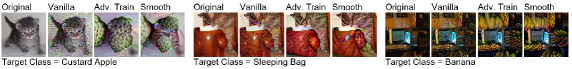
Figure 1: Large-$\epsilon$ targeted adversarial examples for a vanilla-trained network, an adversarially trained network, and a smoothed network. Adversarial examples for both robust classifiers visually resemble the targeted class, while adversarial examples for the vanilla classifier do not. All of these adversarial examples have perturbation size $\epsilon=40$ (on images with pixels scaled to $[0,1]$).

Randomized smoothing

Across many studies, adversarially-trained neural networks have proven empirically successful at resisting adversarial attacks within the threat model in which they were trained [16, 17]. Unfortunately, when the networks are large and expressive, no known algorithms are able to provably certify this robustness [18], leaving open the possibility that they will be vulnerable to better adversarial attacks developed in the future.

For this reason, a distinct approach to robustness called randomized smoothing has recently gained traction in the literature [5, 6, 7, 8]. In the $\ell_{2}$-robust version of randomized smoothing, the robust classifier $\hat{f}_{\sigma}:\mathbb{R}^{d}\to\mathbb{R}^{k}$ is a smoothed neural network of the form:

$$\hat{f}_{\sigma}(\mathbf{x})=\mathbb{E}_{\boldsymbol{\varepsilon}\sim\mathcal{N}(0,\sigma^{2}I)}[f(\mathbf{x}+\boldsymbol{\varepsilon})]$$ (1)

where $f:\mathbb{R}^{d}\to\mathbb{R}^{k}$ is a neural network (ending in a softmax) called the base network. In other words, $\hat{f}_{\sigma}(\mathbf{x})$, the smoothed network’s predicted scores at $\mathbf{x}$, is the weighted average of $f$ within the neighborhood around $\mathbf{x}$, where points are weighted according to an isotropic Gaussian centered at $\mathbf{x}$ with variance $\sigma^{2}$. A disadvantage of randomized smoothing is that the smoothed network $\hat{f}_{\sigma}$ cannot be evaluated exactly, due to the expectation in (1), and instead must approximated via Monte Carlo sampling. However, by computing $\hat{f}_{\sigma}(\mathbf{x})$ one can obtain a guarantee that $\hat{f}_{\sigma}$’s prediction is constant within an $\ell_{2}$ ball around $\mathbf{x}$; in contrast, it is not currently possible to obtain such certificates using neural network classifiers. See Appendix B for more background on randomized smoothing.

How to best train the base network $f$ to maximize the certified accuracy of the smoothed network $\hat{f}_{\sigma}$ remains an open question in the literature. In [5, 7], the base network $f$ was trained with Gaussian data augmentation. However, [19, 6] showed that training $f$ instead using stability training [20] resulted in substantially higher certified accuracy, and [8] showed that training $f$ by adversarially training $\hat{f}_{\sigma}$ also outperformed Gaussian data augmentation. Our main experiments use a base network trained with Gaussian data augmentation. In Appendix C we compare against the network from [8].

2 Experiments

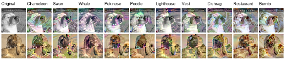
Figure 2: Large-$\epsilon$ adversarial examples for a smoothed neural network. Each row is a (random) starting image, each column is a (random) target class. See Figures 5-6 in Appendix A for more.

In this paper, we show that smoothed neural networks exhibit perceptually-aligned gradients. By design, our experiments mirror those conducted in [10]. To begin, we synthesize large-$\epsilon$ targeted adversarial examples for a smoothed ($\sigma=0.5)$ ResNet-50 trained on ImageNet [21, 22]. Given some source image $\mathbf{x}_{0}$, we used projected gradient descent (PGD) to find an image $\mathbf{x}^{*}$ within $\ell_{2}$ distance $\epsilon$ of $\mathbf{x}_{0}$ that the smoothed network $\hat{f}_{\sigma}$ classifies confidently as target class $t$. Specifically, decomposing $f$ as $f(\mathbf{x})=\operatorname*{softmax}(\operatorname*{logits}(\mathbf{x}))$, we solve the problem:

$$\mathbf{x}^{*}=\operatorname*{arg\,max}_{\mathbf{x}:\;\|\mathbf{x}-\mathbf{x}_{0}\|\leq\epsilon}\mathbb{E}_{\boldsymbol{\varepsilon}\sim\mathcal{N}(0,\sigma^{2}I)}[\operatorname*{logits}(\mathbf{x}+\boldsymbol{\varepsilon})_{t}].$$ (2)

We find that optimizing (2) yields visually more compelling results than minimizing the cross-entropy loss of $\hat{f}_{\sigma}$. See Appendix C for a comparison between (2) and the cross-entropy approach.

The gradient of the objective (2) cannot be computed exactly, due to the expectation over $\boldsymbol{\varepsilon}$, so we instead used an unbiased estimator obtained by sampling $N=20$ noise vectors $\boldsymbol{\varepsilon}_{1},\ldots,\boldsymbol{\varepsilon}_{N}\sim\mathcal{N}(0,\sigma^{2}I)$ and computing the average gradient $\frac{1}{N}\sum_{i=1}^{N}\nabla_{\mathbf{x}}\operatorname*{logits}(\mathbf{x}+\boldsymbol{\varepsilon}_{i})_{t}$.

Figure 1 depicts large-$\epsilon$ targeted adversarial examples for a vanilla-trained neural network, an adversarially trained network [4], and a smoothed network. Observe that the adversarial examples for the vanilla network do not take on coherent features of the target class, while the adversarial examples for both robust networks do. Figure 2 shows large-$\epsilon$ targeted adversarial examples synthesized for the smoothed network for a variety of different target classes.

Next, as in [10], we use the smoothed network to class-conditionally synthesize images. To generate an image from class $t$, we sample a seed image $\mathbf{x}_{0}$ from a multivariate Gaussian fit to images from class $t$, and then we iteratively take gradient steps to maximize the score of class $t$ using objective (2). Figure 3 shows two images synthesized in this way from each of seven ImageNet classes. The synthesized images appear visually similar to instances of the target class, though they often lack global coherence — the synthesized solar dish includes multiple overlapping solar dishes.

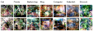
Figure 3: Class-conditional image synthesis using a smoothed NN. To synthesize an image from class $t$, we sampled a seed image from a multivariate Gaussian fit to images from class $t$, and then performed PGD to maximize the score of class $t$. Figures 7-8 in Appendix A have more examples.

Noise Level $\sigma$

Smoothed neural networks have a hyperparameter $\sigma$ which controls a robustness/accuracy tradeoff: when $\sigma$ is high, the smoothed network is more robust, but less accurate [5, 7]. We investigated the effect of $\sigma$ on the perceptual quality of generated images. Figure 4 shows large-$\epsilon$ adversarial examples crafted for smoothed networks with $\sigma$ varying in $\{0.25,0.50,1.00\}$. Observe that when $\sigma$ is large, PGD tends to paint single instance of the target class; when $\sigma$ is small, PGD tends to add spatially scattered features.

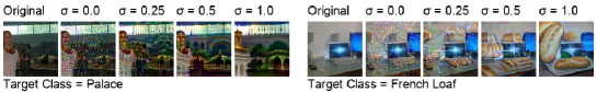
Figure 4: Large-$\epsilon$ adversarial examples crafted for smoothed neural networks with different settings of the smoothing scale hyperparameter $\sigma$. More examples are in Figures 9-11 in Appendix A.

Other concerns

In Appendix C, we study the effects of the following factors on the perceptual quality of the generated images: the number of Monte Carlo noise samples $N$, the loss function used for PGD, and whether the base network $f$ is trained using Gaussian data augmentation [5, 7] or SmoothAdv [8].

Appendix A Additional images

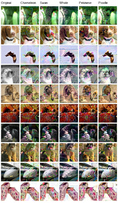
Figure 5: Large-$\epsilon$ adversarial examples for a smoothed neural network (part 1 / 2). Each row is a randomly chosen starting image, each column is a randomly chosen target class.

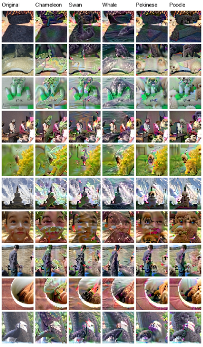
Figure 6: Large-$\epsilon$ adversarial examples for a smoothed neural network (part 2 / 2). Each row is a randomly chosen starting image, each column is a randomly chosen target class.

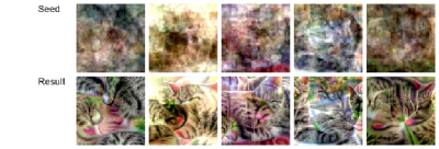
(a) cat

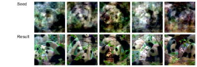
(b) panda

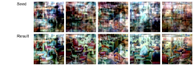
(c) barber shop

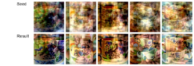
(d) mug

Figure 7: Class-conditional synthesized images (part 1 / 2). To synthesize an image from class $t$, we sampled a seed image from a multivariate Gaussian distribution fit to class $t$, and then performed PGD to maximize the score which a smoothed neural network assigns to class $t$. The top row shows the seed image, the bottom row shows the result of PGD.

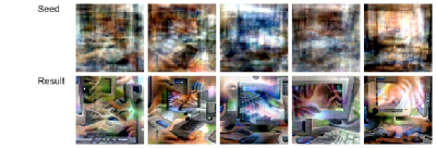
(a) computer

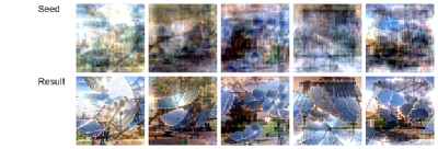
(b) solar dish

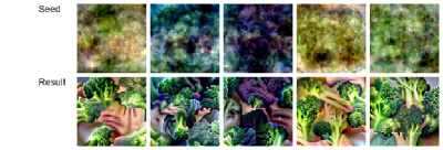
(c) broccoli

Figure 8: Class-conditional synthesized images (part 2 / 2). To synthesize an image from class $t$, we sampled a starting image from a multivariate Gaussian distribution fit to class $t$, and then performed PGD to maximize the score which a smoothed neural network assigns to class $t$. The top row shows the seed image, the bottom row shows the result of PGD.

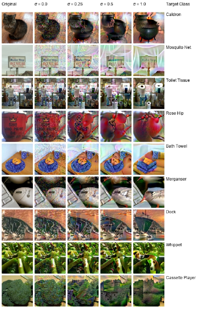
Figure 9: Large-$\epsilon$ adversarial examples crafted for smoothed neural networks with different settings of the smoothing scale hyperparameter $\sigma$ (part 1 / 3). Images and target classes were randomly chosen. When $\sigma$ is large, the adversary tends to paint a single, coherent instance of the target class; when $\sigma$ is small, the adversary tends to paint scattered features of the target class. Note that $\sigma=0.0$ corresponds to a vanilla-trained network.

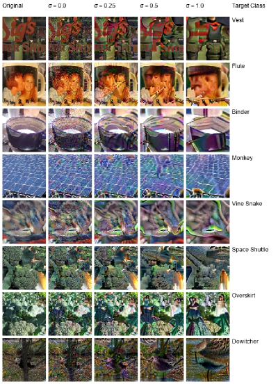
Figure 10: Large-$\epsilon$ adversarial examples crafted for smoothed neural networks with different settings of the smoothing scale hyperparameter $\sigma$ (part 2 / 3). Images and target classes were randomly chosen. When $\sigma$ is large, the adversary tends to paint a single, coherent instance of the target class; when $\sigma$ is small, the adversary tends to paint scattered features of the target class. Note that $\sigma=0.0$ corresponds to a vanilla-trained network.

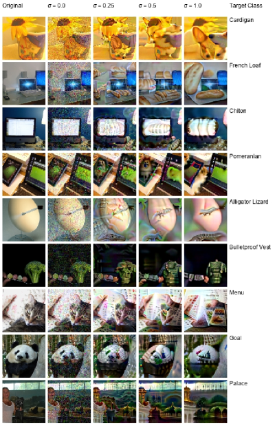
Figure 11: Large-$\epsilon$ adversarial examples crafted for smoothed neural networks with different settings of the smoothing scale hyperparameter $\sigma$ (part 3 / 3). Images and target classes were randomly chosen. When $\sigma$ is large, the adversary tends to paint a single, coherent instance of the target class; when $\sigma$ is small, the adversary tends to paint scattered features of the target class. Note that $\sigma=0.0$ corresponds to a vanilla-trained network.

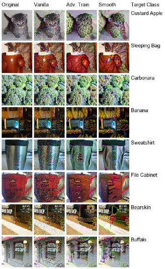
Figure 12: Large-$\epsilon$ targeted adversarial examples for a vanilla-trained network, an adversarially trained network [4], and a smoothed network. Adversarial examples for both robust classifiers visually resemble the targeted class, while adversarial examples for the vanilla classifier do not. All of these adversarial examples have perturbation size $\epsilon=40$ (on images with pixels scaled to $[0,1]$).

Appendix B Randomized Smoothing

Randomized smoothing is relatively new to the literature, and few comprehensive references exist. Therefore, in this appendix, we review some basic aspects of the technique.

Preliminaries

Randomized smoothing refers to a class of adversarial defenses in which the robust classifier $g:\mathbb{R}^{d}\to[k]$ that maps from an input in $\mathbb{R}^{d}$ to a class in $[k]:=\{1,\ldots,k\}$ is defined as:

$$g(\mathbf{x})=\operatorname*{arg\,max}_{y\in[k]}\;\mathbb{E}_{T}[f(T(\mathbf{x}))]_{y}.$$

Here, $f:\mathbb{R}^{d}\to\Delta_{k}$ is a neural network “base classifier” which maps from an input in $\mathbb{R}^{d}$ to a vector of class scores in $\Delta_{k}:=\{\mathbf{z}\in\mathbb{R}^{k}:\mathbf{z}\geq 0,\sum_{j=1}^{k}z_{j}=1\}$, the probability simplex of non-negative $k$-vectors that sum to 1. $T$ is a randomization operation which randomly corrupts inputs in $\mathbb{R}^{d}$ to other inputs in $\mathbb{R}^{d}$, i.e. for any $\mathbf{x}$, $T(\mathbf{x})$ is a random variable.

Intuitively, the score which the smoothed classifier $g$ assigns to class $y$ for the input $\mathbf{x}$ is defined to be the expected score that the base classifier $f$ assigns to the class $y$ for the random input $T(\mathbf{x})$.

The requirement that $f$ returns outputs in the probability simplex $\Delta_{k}$ can be satisfied in either of two ways. In the “soft smoothing” formulation (presented in the main paper), $f$ is a neural network which ends in a softmax. In the “hard smoothing” formulation, $f$ returns the indicator vector for a particular class, i.e. a length-$k$ vector with one 1 and the rest zeros, without exposing the intermediate class scores. In the hard smoothing formulation, since the expectation of an indicator function is a probability, the smoothed classifier $g(\mathbf{x})$ can be interpreted as returning the most probable prediction by the classifier $f$ over the random variable $T(\mathbf{x})$. Note that no papers have yet studied soft smoothing as a certified defense, though [8] approximated a hard smoothing classifier with the corresponding soft classifier in order to attack it.

When the base classifier $f$ is a neural network, the smoothed classifier $g$ cannot be evaluated exactly, since it is not possible to exactly compute the expectation of a neural network’s prediction over a random input. However, by repeatedly sampling the random vector $f(T(\mathbf{x}))$, one can obtain upper and lower bounds on the expected value of each entry of that vector, which hold with high probability over the sampling procedure. In the hard smoothing case, since each entry of $f(T(\mathbf{x}))$ is a Bernoulli random variable, one can use standard Bernoulli confidence intervals like the Clopper-Pearson, as in [5, 7]. In the soft smoothing case, since each entry of $f(T(\mathbf{x}))$ is bounded in $[0,1]$, one can use Hoeffding-style concentration inequalities to derive high-probability confidence intervals for the entries of $f(T(\mathbf{x}))$ .

Gaussian smoothing

When $T$ is an additive Gaussian corruption,

$$T(\mathbf{x})=\mathbf{x}+\boldsymbol{\varepsilon},\quad\boldsymbol{\varepsilon}\sim\mathcal{N}(0,\sigma^{2}I),$$

the robust classifier $g:\mathbb{R}^{d}\to[k]$ is given by:

$$g(\mathbf{x})=\;\operatorname*{arg\,max}_{j\in[k]}\;\hat{f}_{\sigma}(\mathbf{x})\quad\text{where}\quad\hat{f}_{\sigma}(\mathbf{x})=\mathbb{E}_{\boldsymbol{\varepsilon}\sim\mathcal{N}(0,\sigma^{2}I)}[f(\mathbf{x}+\boldsymbol{\varepsilon})].$$ (3)

Gaussian-smoothed classifiers are certifiably robust under the $\ell_{2}$ norm: for any input $\mathbf{x}$, if we know $\hat{f}_{\sigma}(\mathbf{x})$, we can certify that $g$’s prediction will remain constant within an $\ell_{2}$ ball around $\mathbf{x}$:

Theorem 1 (Extension to “soft smoothing” of Theorem 1 from [7]; see also Appendix A in [8]).

Let $f:\mathbb{R}^{d}\to\Delta_{k}$ be any function, and define $g$ and $\hat{f}_{\sigma}$ as in (3). For some $\mathbf{x}\in\mathbb{R}^{d}$, let $y_{1},y_{2}\in[k]$ be the indices of the largest and second-largest entries of $\hat{f}_{\sigma}(\mathbf{x})$. Then $g(\mathbf{x}+\boldsymbol{\delta})=y_{1}$ for any $\boldsymbol{\delta}$ with

$$\|\boldsymbol{\delta}\|_{2}\leq\frac{\sigma}{2}\left(\Phi^{-1}(\hat{f}_{\sigma}(\mathbf{x})_{y_{1}})-\Phi^{-1}(\hat{f}_{\sigma}(\mathbf{x})_{y_{2}})\right).$$

Theorem 1 is easy to prove using the following mathematical fact:

Lemma 2 (Lemma 2 from [8], Lemma 1 from [23]).

Let $h:\mathbb{R}^{d}\to[0,1]$ be any function, and define its Gaussian convolution $\hat{h}_{\sigma}$ as $\hat{h}_{\sigma}(\mathbf{x})=\mathbb{E}_{\boldsymbol{\varepsilon}\sim\mathcal{N}(0,\sigma^{2}I)}[h(\mathbf{x}+\boldsymbol{\varepsilon})]$. Then, for any input $\mathbf{x}\in\mathbb{R}^{d}$ and any perturbation $\boldsymbol{\delta}\in\mathbb{R}^{d}$,

$$\Phi\left(\Phi^{-1}(\hat{h}_{\sigma}(\mathbf{x}))-\frac{\|\boldsymbol{\delta}\|_{2}}{\sigma}\right)\leq\hat{h}_{\sigma}(\mathbf{x}+\boldsymbol{\delta})\leq\Phi\left(\Phi^{-1}(\hat{h}_{\sigma}(\mathbf{x}))+\frac{\|\boldsymbol{\delta}\|_{2}}{\sigma}\right).$$

Intuitively, Lemma 2 says that $\hat{h}_{\sigma}(\mathbf{x}+\boldsymbol{\delta})$ cannot be too much larger or too much smaller than $\hat{h}_{\sigma}(\mathbf{x})$. If this has the feel of a Lipschitz guarantee, there is good reason: Lemma 2 is equivalent to the statement that the function $\mathbf{x}\mapsto\Phi^{-1}(\hat{h}_{\sigma}(\mathbf{x}))$ is $1/\sigma$-Lipschitz.

Theorem 1 is a direct consequence of Lemma 2:

Proof of Theorem 1.

Since the outputs of $\hat{f}_{\sigma}$ live in the probability simplex, for each class $j$ the function $\hat{f}_{\sigma}(\cdot)_{j}$ has output bounded in $[0,1]$, and hence can be viewed as a function $\hat{h}_{\sigma}$ for which the condition of Lemma 2 applies.

Therefore, from applying Lemma 2 to $\hat{f}_{\sigma}(\cdot)_{y_{1}}$, we know that:

$$\hat{f}_{\sigma}(\mathbf{x}+\boldsymbol{\delta})_{y_{1}}\geq\Phi\left(\Phi^{-1}(\hat{f}_{\sigma}(\mathbf{x})_{y_{1}})-\frac{\|\boldsymbol{\delta}\|_{2}}{\sigma}\right)$$

and, for any $j$, from applying Lemma 2 to $\hat{f}_{\sigma}(\cdot)_{j}$, we know that:

$$\Phi\left(\Phi^{-1}(\hat{f}_{\sigma}(\mathbf{x})_{j})+\frac{\|\boldsymbol{\delta}\|_{2}}{\sigma}\right)\geq\hat{f}_{\sigma}(\mathbf{x}+\boldsymbol{\delta})_{j}.$$

Combining these two results, it follows that a sufficient condition for $\hat{f}_{\sigma}(\mathbf{x}+\boldsymbol{\delta})_{y_{1}}\geq\hat{f}_{\sigma}(\mathbf{x}+\boldsymbol{\delta})_{j}$ is:

$$\Phi\left(\Phi^{-1}(\hat{f}_{\sigma}(\mathbf{x})_{y_{1}})-\frac{\|\boldsymbol{\delta}\|_{2}}{\sigma}\right)\geq\Phi\left(\Phi^{-1}(\hat{f}_{\sigma}(\mathbf{x})_{j})+\frac{\|\boldsymbol{\delta}\|_{2}}{\sigma}\right),$$

or equivalently,

$$\|\boldsymbol{\delta}\|_{2}\leq\frac{\sigma}{2}(\Phi^{-1}(\hat{f}_{\sigma}(\mathbf{x})_{y_{1}}-\Phi^{-1}(\hat{f}_{\sigma}(\mathbf{x})_{j})).$$

Hence, we can conclude that $\hat{f}_{\sigma}(\mathbf{x}+\boldsymbol{\delta})_{y_{1}}\geq\max_{j\neq y_{1}}\hat{f}_{\sigma}(\mathbf{x}+\boldsymbol{\delta})_{j}$ so long as

$$\|\boldsymbol{\delta}\|_{2}\leq\min_{j\neq y_{1}}\left\{\frac{\sigma}{2}(\Phi^{-1}(\hat{f}_{\sigma}(\mathbf{x})_{y_{1}}-\Phi^{-1}(\hat{f}_{\sigma}(\mathbf{x})_{j}))\right\}=\frac{\sigma}{2}(\Phi^{-1}(\hat{f}_{\sigma}(\mathbf{x})_{y_{1}}-\Phi^{-1}(\hat{f}_{\sigma}(\mathbf{x})_{y_{2}}))$$

∎

Training

Given a dataset, a base classifier architecture, and a smoothing level $\sigma>0$, it currently an active research question to figure out the best way to train the base classifier $f$ so that the smoothed classifier $g$ will attain high certified or empirical robust accuracies. The original randomized smoothing paper [5] proposed training $f$ with Gaussian data augmentation and the standard cross-entropy loss. However, [8] and [6, 19] showed that alternative training schemes yield substantial gains in certified accuracy. In particular, [8] proposed training $f$ by performing adversarial training on $g$, and [6, 19] proposed training $f$ via stability training [20].

Related work

Gaussian smoothing was first proposed as a certified adversarial defense by [5] under the name “PixelDP,” though similar techniques had been proposed earlier as a heuristic defenses in [24, 25]. Subsequently, [6] proved a stronger robustness guarantee, and finally [7] derived the tightest possible robustness guarantee in the “hard smooothing” case, which was extended to the “soft smoothing” case by [23, 8].

Concurrently, [26] proved a robustness guarantee in $\ell_{\infty}$ norm for Gaussian smoothing; however, since Gaussian smoothing specifically confers $\ell_{2}$ (not $\ell_{\infty}$) robustness [7], the certified accuracy numbers reported in [26] were weak.

[27] gave theoretical and empirical arguments for an adversarial defense similar to randomized smoothing, but did not position their method as a certified defense.

[28] have extended randomized smoothing beyond Gaussian noise / $\ell_{2}$ norm by proposing a randomization scheme which allows for certified robustness in the $\ell_{0}$ norm.

Appendix C Details on Generating Images

This appendix details the procedure used to generate the images that appeared in this paper.

As in [10], to generate an image $\mathbf{x}^{*}\in\mathbb{R}^{d}$ near the starting image $\mathbf{x}_{0}$ that is classified by a smoothed neural network $\hat{f}_{\sigma}$ as some target class $t$, we use projected steepest descent to solve the optimization problem:

$$\mathbf{x}^{*}=\operatorname*{arg\,min}_{\mathbf{x}:\;\|\mathbf{x}-\mathbf{x}_{0}\|_{2}\leq\epsilon}\;L(\hat{f}_{\sigma},\mathbf{x},t)$$ (4)

where $L$ is a loss function measuring the extent to which $\hat{f}_{\sigma}$ classifies $\mathbf{x}$ as class $t$.

The two big choices which need to be made are: which loss function to use, and how to compute its gradient?

Loss functions for adversarially-trained networks

We first review two loss functions for generating images using adversarially-trained neural networks. Our loss functions for smoothed neural networks (presented below) are inspired by these.

The first is the cross-entropy loss. If $f^{\text{adv}}:\mathbb{R}^{d}\to\Delta_{k}$ is an (adversarially trained) neural network classifier that ends in a softmax layer (so that its output lies on the probability simplex $\Delta_{k}$), the cross-entropy loss is defined as:

$$L_{\text{CE}}(f^{\text{adv}},\mathbf{x},t):=-\log f^{\text{adv}}(\mathbf{x})_{t}.$$

The second is the “target class max” (TCM) loss. If we write $f^{\text{adv}}$ as $f^{\text{adv}}(\mathbf{x})=\operatorname*{softmax}(\operatorname*{logits}(\mathbf{x}))$, where $\operatorname*{logits}:\mathbb{R}^{d}\to\mathbb{R}^{k}$ is $f^{\text{adv}}$ minus the final softmax layer, then the TCM loss is defined as:

$$L_{\text{TCM}}(f^{\text{adv}},\mathbf{x},t):=-\operatorname*{logits}(\mathbf{x})_{t}.$$

In other words, minimizing $L_{\text{TCM}}$ will maximize the score that $\operatorname*{logits}$ assigns to class $t$.

Since $f^{\text{adv}}$ is just a neural network, computing the gradients of these loss functions can be easily done using automatic differentiation. (The situation is more complicated for smoothed neural networks.)

We note that [10] used $L_{\text{CE}}$ in their experiments.

Loss functions for smoothed networks

Our loss functions for smoothed neural networks are inspired by those described above for adversarially trained networks. If $\hat{f}_{\sigma}$ is a smoothed neural network of the form $\hat{f}_{\sigma}(\mathbf{x})=\mathbb{E}_{\boldsymbol{\varepsilon}\sim\mathcal{N}(0,\sigma^{2}I)}[f(\mathbf{x}+\boldsymbol{\varepsilon})]$, with $f$ a neural network that ends in a softmax layer, then the cross-entropy loss is defined as:

$$L_{\text{CE}}(\hat{f}_{\sigma},\mathbf{x},t):=-\log\hat{f}_{\sigma}(\mathbf{x})_{t}=-\log\mathbb{E}_{\boldsymbol{\varepsilon}\sim\mathcal{N}(0,\sigma^{2}I)}[f(\mathbf{x}+\boldsymbol{\varepsilon})_{t}].$$ (5)

If we decompose $f$ as $f(\mathbf{x})=\operatorname*{softmax}(\operatorname*{logits}(\mathbf{x}))$, where $\operatorname*{logits}:\mathbb{R}^{d}\to\mathbb{R}^{k}$ is $f$ minus the softmax layer, then the TCM loss is defined as:

$$L_{\text{TCM}}(\hat{f}_{\sigma},\mathbf{x},t):=-\mathbb{E}_{\boldsymbol{\varepsilon}\sim\mathcal{N}(0,\sigma^{2}I)}[\operatorname*{logits}(\mathbf{x}+\boldsymbol{\varepsilon})_{t}].$$ (6)

In other words, minimizing $L_{\text{TCM}}$ will maximize the expected logit of class $t$ for the random input $\mathbf{x}+\boldsymbol{\varepsilon}$

Gradient estimators

To solve problem (4) using PGD, we need to be able to compute the gradient of the objective w.r.t $\mathbf{x}$. However, for smoothed neural networks, it is not possible to exactly compute the gradient of either $L_{\text{CE}}$ or $L_{\text{TCM}}$. We therefore must resort to gradient estimates obtained using Monte Carlo sampling.

For $L_{\text{TCM}}$, we use the following unbiased gradient estimator:

$$\nabla_{\mathbf{x}}L_{\text{TCM}}(\hat{f}_{\sigma},\mathbf{x},t)\approx-\frac{1}{N}\sum_{i=1}^{N}\nabla_{\mathbf{x}}\operatorname*{logits}(\mathbf{x}+\boldsymbol{\varepsilon}_{i})_{t},\quad\boldsymbol{\varepsilon}_{i}\sim\mathcal{N}(0,\sigma^{2}I)$$

This estimator is unbiased since

$$\mathbb{E}_{\boldsymbol{\varepsilon}_{1},\ldots,\boldsymbol{\varepsilon}_{N}\sim\mathcal{N}(0,\sigma^{2}I)}\left[-\frac{1}{N}\sum_{i=1}^{N}\nabla_{\mathbf{x}}\operatorname*{logits}(\mathbf{x}+\boldsymbol{\varepsilon}_{i})_{t}\right] =\mathbb{E}_{\boldsymbol{\varepsilon}\sim\mathcal{N}(0,\sigma^{2}I)}\left[-\nabla_{\mathbf{x}}\operatorname*{logits}(\mathbf{x}+\boldsymbol{\varepsilon})_{t}\right]$$

$$=\nabla_{\mathbf{x}}\;\mathbb{E}_{\boldsymbol{\varepsilon}\sim\mathcal{N}(0,\sigma^{2}I)}\left[-\operatorname*{logits}(\mathbf{x}+\boldsymbol{\varepsilon})_{t}\right].$$

For $L_{\text{CE}}$, we are unaware of any unbiased gradient estimator, so, following [8], we use the following biased “plug-in” gradient estimator:

$$\nabla_{\mathbf{x}}L_{\text{CE}}(\hat{f}_{\sigma},\mathbf{x},t)\approx\nabla_{\mathbf{x}}\left[-\log\left(\frac{1}{N}\sum_{i=1}^{N}f(\mathbf{x}+\boldsymbol{\varepsilon}_{i})_{t}\right)\right],\quad\boldsymbol{\varepsilon}_{i}\sim\mathcal{N}(0,\sigma^{2}I)$$

Experimental comparison between loss functions

Figure 13 shows large-$\epsilon$ adversarial examples crafted for a smoothed neural network using both $L_{\text{TCM}}$ and $L_{\text{CE}}$. The adversarial examples crafted using $L_{\text{TCM}}$ seem to better perceptually resemble the target class. Therefore, in this work we primarily use $L_{\text{TCM}}$.

Experimental comparison between training procedures

For most of the figures in this paper, we used a base classifier from [7] trained using Gaussian data augmentation. However, in Figures 15-17, we compare large-$\epsilon$ adversarial examples for this base classifier to those synthesized for a base classifier trained using the SmoothAdv procedure from [8], which was shown in that paper to attain much better certified accuracies than the network from [7]. We find that there does not seem to be a large difference in the perceptual quality of the generated images. Therefore, throughout this paper we used the network from [7], since we wanted to emphasize that perceptually-aligned gradients arise even with robust classifiers that do not involve adversarial training of any kind.

Experimental study of number of Monte Carlo samples

One important question is how many Monte Carlo samples $N$ are needed when computing the gradient of $L_{\text{TCM}}$ or $L_{\text{CE}}$. In Figure 14 we show large-$\epsilon$ adversarial examples synthesized using $N\in\{1,5,20,25,50,75\}$ Monte Carlo samples. There does not seem to be a large difference between using $N=20$ samples or using more than 20. Images synthesized using $N=1$ samples do appear a bit less developed than the others (e.g. the terrier with $N=1$ is has fewer ears than when $N$ is large.) In this work, we primarily used $N=20$.

Hyperparameters

The following table shows the hyperparameter settings for all of the figures in this paper.

Figure	$\sigma$	number of PGD steps	$\epsilon$	PGD step size	$N$
1, 12	0.5	300	40.0	2.8 (vanilla), 0.7	20
2	0.5	300	40.0	0.7	20
3	0.5	300	40.0	0.7	20
4, 9-11	vary	300	40.0	2.8 ($\sigma$ = 0), 0.7	20
15-17	0.5, 1.0	300	40.0	0.7	20
13	0.5	300	40.0	2.0 (CE), 0.7	20
14	0.5	300	40.0	0.7	vary

Note that Figures 1 and 12 only use stepSize = 2.8 in the Vanilla column, Figure 13 only uses stepSize = 2.0 in the C-E Loss column, and Figures 4 and 9-11 only use stepSize = 2.8 for $\sigma$ = 0.

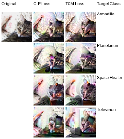
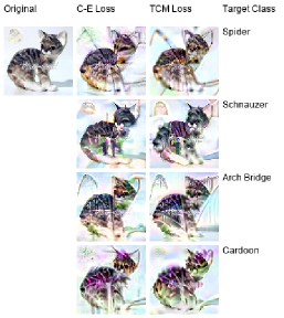
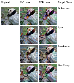
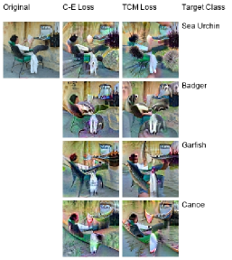
Figure 13: Here, we compare the perceptual quality of large-$\epsilon$ adversarial examples (for a smoothed neural network) crafted using the cross-entropy loss $L_{\text{CE}}$ to those crafted using the target class max $L_{\text{TCM}}$ loss. Observe that adversarial examples crafted using the TCM loss seem to better resemble the targeted class. For this reason, we used the TCM loss function throughout this paper.

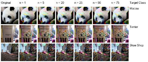
Figure 14: Large-$\epsilon$ adversarial examples for a smoothed neural network crafted using different settings of the parameter $N$, the number of Monte Carlo samples used for gradient estimation.

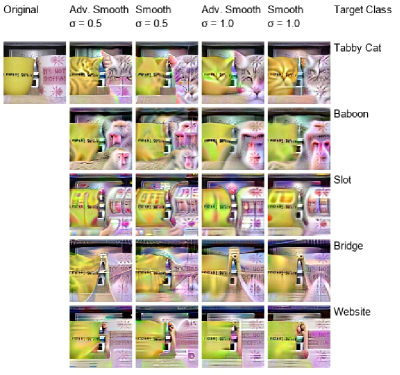
Figure 15: We compare (part 1/3) large-$\epsilon$ targeted adversarial examples for smoothed networks trained using Gaussian data augmentation [5, 7] (columns “Smooth”) to those for smoothed networks trained using the SmoothAdv algorithm of [8], i.e. adversarial training on the smoothed classifier (columns “Adv. Smooth”).

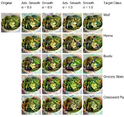
Figure 16: We compare (part 2/3) large-$\epsilon$ targeted adversarial examples for smoothed networks trained using Gaussian data augmentation [5, 7] (columns “Smooth”) to those for smoothed networks trained using the SmoothAdv algorithm of [8], i.e. adversarial training on the smoothed classifier (columns “Adv. Smooth”).

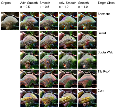
Figure 17: We compare (part 3/3) large-$\epsilon$ targeted adversarial examples for smoothed networks trained using Gaussian data augmentation [5, 7] (columns “Smooth”) to those for smoothed networks trained using the SmoothAdv algorithm of [8], i.e. adversarial training on the smoothed classifier (columns “Adv. Smooth”).

References

- Szegedy et al. [2014] Christian Szegedy, Wojciech Zaremba, Ilya Sutskever, Joan Bruna, Dumitru Erhan, Ian Goodfellow, and Rob Fergus. Intriguing properties of neural networks. In International Conference on Learning Representations, 2014.
- Biggio et al. [2013] Battista Biggio, Igino Corona, Davide Maiorca, Blaine Nelson, Nedim Šrndić, Pavel Laskov, Giorgio Giacinto, and Fabio Roli. Evasion attacks against machine learning at test time. Joint European Conference on Machine Learning and Knowledge Discovery in Database, 2013.
- Kurakin et al. [2016] Alexey Kurakin, Ian Goodfellow, and Samy Bengio. Adversarial machine learning at scale. arXiv preprint arXiv:1611.01236, 2016.
- Madry et al. [2018] Aleksander Madry, Aleksandar Makelov, Ludwig Schmidt, Dimitris Tsipras, and Adrian Vladu. Towards deep learning models resistant to adversarial attacks. In International Conference on Learning Representations, 2018.
- Lecuyer et al. [2019] M. Lecuyer, V. Atlidakis, R. Geambasu, D. Hsu, and S. Jana. Certified robustness to adversarial examples with differential privacy. In IEEE Symposium on Security and Privacy (SP), 2019.
- Li et al. [2019] Bai Li, Changyou Chen, Wenlin Wang, and Lawrence Carin. Certified adversarial robustness with additive gaussian noise. In Advances in Neural Information Processing Systems (NeurIPS), 2019.
- Cohen et al. [2019] Jeremy Cohen, Elan Rosenfeld, and Zico Kolter. Certified adversarial robustness via randomized smoothing. In Proceedings of the 36th International Conference on Machine Learning, 2019.
- Salman et al. [2019a] Hadi Salman, Greg Yang, Jerry Li, Pengchuan Zhang, Huan Zhang, Ilya Razenshteyn, and Sebastien Bubeck. Provably robust deep learning via adversarially trained smoothed classifiers. In Advances in Neural Information Processing Systems (NeurIPS), 2019a.
- Tsipras et al. [2019] Dimitris Tsipras, Shibani Santurkar, Logan Engstrom, Alexander Turner, and Aleksander Madry. Robustness may be at odds with accuracy. In International Conference on Learning Representations, 2019. URL https://openreview.net/forum?id=SyxAb30cY7.
- Santurkar et al. [2019] Shibani Santurkar, Dimitris Tsipras, Brandon Tran, Andrew Ilyas, Logan Engstrom, and Aleksander Madry. Image synthesis with a single (robust) classifier. In Advances in Neural Information Processing Systems (NeurIPS), 2019.
- Engstrom et al. [2019] Logan Engstrom, Andrew Ilyas, Shibani Santurkar, Dimitris Tsipras, Brandon Tran, and Aleksander Madry. Adversarial robustness as a prior for learned representations. arXiv preprint arXiv:1906.00945, 2019.
- Olah et al. [2017] Chris Olah, Alexander Mordvintsev, and Ludwig Schubert. Feature visualization. Distill, 2017. doi: 10.23915/distill.00007. https://distill.pub/2017/feature-visualization.
- Nguyen et al. [2015] Anh Mai Nguyen, Jason Yosinski, and Jeff Clune. Deep neural networks are easily fooled: High confidence predictions for unrecognizable images. 2015 IEEE Conference on Computer Vision and Pattern Recognition (CVPR), 2015.
- Mahendran and Vedaldi [2015] Aravindh Mahendran and Andrea Vedaldi. Understanding deep image representations by inverting them. 2015 IEEE Conference on Computer Vision and Pattern Recognition (CVPR), Jun 2015. doi: 10.1109/cvpr.2015.7299155. URL http://dx.doi.org/10.1109/CVPR.2015.7299155.
- Øygard [2015] Audun M. Øygard. Visualizing googlenet claasses. https://www.auduno.com/2015/07/29/visualizing-googlenet-classes/, 2015. [Online; accessed 30-August-2019].
- Athalye et al. [2018] Anish Athalye, Nicholas Carlini, and David Wagner. Obfuscated gradients give a false sense of security: Circumventing defenses to adversarial examples. In Proceedings of the 35th International Conference on Machine Learning, 2018.
- Brendel et al. [2019] Wieland Brendel, Jonas Rauber, Matthias Kümmerer, Ivan Ustyuzhaninov, and Matthias Bethge. Accurate, reliable and fast robustness evaluation. In Advances in Neural Information Processing Systems (NeurIPS), 2019.
- Salman et al. [2019b] Hadi Salman, Greg Yang, Huan Zhang, Cho-Jui Hsieh, and Pengchuan Zhang. A convex relaxation barrier to tight robustness verification of neural networks. In Advances in Neural Information Processing Systems (NeurIPS), 2019b.
- Carmon et al. [2019] Y. Carmon, A. Raghunathan, L. Schmidt, P. Liang, and J. C. Duchi. Unlabeled data improves adversarial robustness. In Advances in Neural Information Processing Systems (NeurIPS), 2019.
- Zheng et al. [2016] Stephan Zheng, Yang Song, Thomas Leung, and Ian J. Goodfellow. Improving the robustness of deep neural networks via stability training. In Computer Vision and Pattern Recognition, 2016.
- He et al. [2016] Kaiming He, Xiangyu Zhang, Shaoqing Ren, and Jian Sun. Deep residual learning for image recognition. 2016 IEEE Conference on Computer Vision and Pattern Recognition (CVPR), Jun 2016.
- Deng et al. [2009] J. Deng, W. Dong, R. Socher, L.-J. Li, K. Li, and L. Fei-Fei. ImageNet: A Large-Scale Hierarchical Image Database. In IEEE Conference on Computer Vision and Pattern Recognition (CVPR), 2009.
- Levine et al. [2019] Alexander Levine, Sahil Singla, and Soheil Feizi. Certifiably robust interpretation in deep learning. arXiv preprint arXiv:1905.12105, 2019.
- Cao and Gong [2017] Xiaoyu Cao and Neil Zhenqiang Gong. Mitigating evasion attacks to deep neural networks via region-based classification. 33rd Annual Computer Security Applications Conference, 2017.
- Liu et al. [2018] Xuanqing Liu, Minhao Cheng, Huan Zhang, and Cho-Jui Hsieh. Towards robust neural networks via random self-ensemble. In The European Conference on Computer Vision (ECCV), September 2018.
- Zhang and Liang [2019] Y. Zhang and P. Liang. Defending against whitebox adversarial attacks via randomized discretization. In Artificial Intelligence and Statistics (AISTATS), 2019.
- Pinot et al. [2019] Rafael Pinot, Laurent Meunier, Alexandre Araujo, Hisashi Kashima, Florian Yger, Cédric Gouy-Pailler, and Jamal Atif. Theoretical evidence for adversarial robustness through randomization. In Advances in Neural Information Processing Systems (NeurIPS), 2019.
- Lee et al. [2019] Guang-He Lee, Yang Yuan, Shiyu Chang, and Tommi S. Jaakkola. A stratified approach to robustness for randomly smoothed classifiers. In Advances in Neural Information Processing Systems (NeurIPS), 2019.