An exactly mass conserving space-time embedded-hybridized discontinuous Galerkin method for the Navier–Stokes equations on moving domains

Abstract

This paper presents a space-time embedded-hybridized discontinuous Galerkin (EHDG) method for the Navier–Stokes equations on moving domains. This method uses a different hybridization compared to the space-time hybridized discontinuous Galerkin (HDG) method we presented previously in (Int. J. Numer. Meth. Fluids 89: 519–532, 2019). In the space-time EHDG method the velocity trace unknown is continuous while the pressure trace unknown is discontinuous across facets. In the space-time HDG method, all trace unknowns are discontinuous across facets. Alternatively, we present also a space-time embedded discontinuous Galerkin (EDG) method in which all trace unknowns are continuous across facets. The advantage of continuous trace unknowns is that the formulation has fewer global degrees-of-freedom for a given mesh than when using discontinuous trace unknowns. Nevertheless, the discrete velocity field obtained by the space-time EHDG and EDG methods, like the space-time HDG method, is exactly divergence-free, even on moving domains. However, only the space-time EHDG and HDG methods result in divergence-conforming velocity fields. An immediate consequence of this is that the space-time EHDG and HDG discretizations of the conservative form of the Navier–Stokes equations are energy stable. The space-time EDG method, on the other hand, requires a skew-symmetric formulation of the momentum advection term to be energy-stable. Numerical examples will demonstrate the differences in solution obtained by the space-time EHDG, EDG, and HDG methods.

1 Introduction

In this paper, we consider the solution of the Navier–Stokes equations on moving and deforming domains. One of the more popular approaches to solve partial differential equations on time-dependent domains is the arbitrary Lagrangian-Eulerian (ALE) class of methods. In the ALE method, the time-varying domain is mapped to a fixed reference domain on which all computations are performed. Although relatively easy to implement, it is known that the ALE method does not automatically satisfy the Geometric Conservation Law (GCL) [1] which requires that the numerical method must reproduce exactly a constant solution. Not satisfying the GCL has consequences for the time-accuracy of the solution [2] and constraints on the numerical method are necessary to enforce this property, e.g., [3, 4].

A different approach to solving PDEs on deforming domains is by space-time methods. In space-time finite element methods, the PDE is discretized simultaneously in space and time by a finite element method. Typically, discontinuous Galerkin (DG) time-stepping methods are employed [5, 6] tensorized with some spatial elemental bases. The space-time finite element method has successfully been applied to the Navier–Stokes equations, e.g., [7, 8, 9, 10, 11]. However, using a continuous spatial basis results in methods that are not locally conservative and which are generally not suited for advection dominated flows.

Using a DG basis in both space and time results in the space-time DG method. This approach was first introduced for compressible flows in [12] and applied later also to incompressible flows [13, 14]. The space-time DG method is locally conservative, can be made of arbitrary order in both space and time, automatically satisfies the GCL, and is well suited for advection dominated flows. Unfortunately, the space-time DG method is computationally costly; a $d$-dimensional time-dependent problem is discretized as a $d+1$-dimensional space-time problem. This results in a significant increase in the number of degrees-of-freedom compared to, for example, a $d$-dimensional DG discretization within an ALE framework.

To address the increase of degrees-of-freedom in a space-time framework, space-time hybridizable discontinuous Galerkin (HDG) methods were introduced in [15, 16]; see also [17] for an analysis of the space-time HDG method for the advection-diffusion equation. HDG methods were first introduced for elliptic problems in [18] to reduce the computational cost of DG methods. This is achieved by introducing additional facet unknowns in such a way that static-condensation, in which cell-wise unknowns are eliminated, is trivial. Since its introduction, the HDG method has successfully been applied to both compressible [19] and incompressible [20, 21, 22, 23, 24, 25, 26, 27, 28] flows.

In [29] we introduced a new space-time HDG method for the Navier–Stokes equations. The novelty of this new space-time HDG method is that the discrete velocity is both exactly divergence-free and divergence-conforming, even on time-dependent domains. A consequence is that the discretization of the conservative form of the Navier–Stokes equations is energy-stable. Additionally, the space-time HDG method is locally mass and momentum conserving.

In the space-time HDG method [29] the discrete velocity and pressure trace unknowns are discontinuous across facets. As previously mentioned, these additional facet unknowns are introduced such that eliminating cell-wise unknowns is trivial. Recently, in [30, 31], an embedded-hybridized discontinuous Galerkin (EHDG) method was introduced for incompressible flows on a fixed domain. In such an approach the discrete velocity trace is continuous across facets while the pressure trace is discontinuous. It was shown in [30] that the EHDG method has fewer global degrees-of-freedom than the HDG method, but retains the advantages of the HDG method, i.e., the discrete velocity is exactly divergence-free and divergence-conforming.

To reduce the number of globally coupled degrees-of-freedom even further, we may take both the velocity and pressure trace unknowns to be continuous across facets. This results in a space-time embedded discontinuous Galerkin (EDG) method. An EDG method for the Navier–Stokes equations on fixed domains was introduced in [22]. Unfortunately, the EDG method results in a discrete velocity that is not divergence-conforming. The EDG method, therefore, requires a skew-symmetric formulation of the momentum advection term to be energy-stable. Furthermore, the EDG method is not locally mass conserving.

Motivated by the advantages the EHDG method has shown for incompressible flows on a fixed mesh [30], in this paper, we introduce a space-time EHDG method for the Navier–Stokes equations on time-dependent domains. We furthermore generalize the EDG method [22] to a space-time formulation suitable for approximating the solution to the Navier–Stokes equations on moving/deforming domains.

The rest of this paper is organized as follows. In section 2 we introduce the Navier–Stokes problem. We present the space-time EHDG and EDG methods in section 3 and discuss the properties of these methods in section 4. We present numerical results in section 5 and draw conclusions in section 6.

2 The Navier–Stokes equations on moving/deforming domains

Let $\Omega(t)\subset\mathbb{R}^{d}$ ($d=2,3$) be a domain which depends continuously on $t\in[0,T]$. We are interested in the solution of the Navier–Stokes equations on the space-time domain $\mathcal{E}\mathrel{\mathop{\mathchar 58\relax}}=\mathinner{\left\{(t,x)\,|\,0<t<T,\,x\in\Omega(t)\right\}}\subset\mathbb{R}^{d+1}$:

$$\partial_{t}u+u\cdot\nabla u-\nu\nabla^{2}u+\nabla p =f \text{in }\mathcal{E},$$ (1a)

$$\nabla\cdot u =0 \text{in }\mathcal{E},$$ (1b)

$$u =0 \text{on }\partial\mathcal{E}^{D},$$ (1c)

$$\mathinner{[n_{t}+u\cdot n-\max(n_{t}+u\cdot n,0)]}u+(p\mathbb{I}-\nu\nabla u)n =g \text{on }\partial\mathcal{E}^{N},$$ (1d)

$$u(0,x) =u_{0}(x) \text{in }\Omega(0),$$ (1e)

where $u\mathrel{\mathop{\mathchar 58\relax}}\mathcal{E}\to\mathbb{R}^{d}$ and $p\mathrel{\mathop{\mathchar 58\relax}}\mathcal{E}\to\mathbb{R}$ are the unknown velocity and kinematic pressure, respectively, $\nu\in\mathbb{R}^{+}$ is the kinematic viscosity, $f\mathrel{\mathop{\mathchar 58\relax}}\mathcal{E}\to\mathbb{R}^{d}$ is a forcing term, $g\mathrel{\mathop{\mathchar 58\relax}}\partial\mathcal{E}^{N}\to\mathbb{R}^{d}$ is boundary data, $u_{0}\mathrel{\mathop{\mathchar 58\relax}}\Omega(0)\to\mathbb{R}^{d}$ the initial divergence-free velocity field, and $\mathbb{I}\in\mathbb{R}^{d\times d}$ is the identity matrix. Furthermore, the boundary of $\mathcal{E}$ is partitioned such that $\partial\mathcal{E}=\partial\mathcal{E}^{D}\cup\partial\mathcal{E}^{N}\cup\Omega(0)\cup\Omega(T)$, where there is no overlap between any two of the four sets. The space-time outward unit normal to $\partial\mathcal{E}$ is denoted by $(n_{t},n)\in\mathbb{R}^{d+1}$, with temporal component $n_{t}\in\mathbb{R}$ and spatial component $n\in\mathbb{R}^{d}$.

3 Discretization

3.1 Notation

We consider a ‘slab-by-slab’ approach to discretize the space-time domain $\mathcal{E}$. For this we partition first the time interval using time levels $0=t^{0}<t^{1}<\cdots<t^{N}=T$. The length of each time interval $I^{n}=(t^{n},t^{n+1})$ is denoted by $\Delta t^{n}=t^{n+1}-t^{n}$. We then define a space-time slab as $\mathcal{E}^{n}=\mathinner{\{(t,x)\in\mathcal{E}\,|\,t\in I^{n}\}}$. At time $t=t_{n}$ we denote $\Omega(t)$ by $\Omega^{n}$. The boundary of a space-time slab $\mathcal{E}^{n}$ is then given by $\Omega^{n}$, $\Omega^{n+1}$ and $\partial\mathcal{E}^{n}\mathrel{\mathop{\mathchar 58\relax}}=\mathinner{\{(t,x)\in\partial\mathcal{E}\,|\,t\in I^{n}\}}$.

We next introduce the triangulation $\mathcal{T}^{n}\mathrel{\mathop{\mathchar 58\relax}}=\mathinner{\left\{\mathcal{K}\right\}}$ of the space-time slab $\mathcal{E}^{n}$, which consists of non-overlapping $(d+1)$-dimensional simplicial space-time elements $\mathcal{K}$. For simplicity we consider the case of matching meshes at the boundary, $\Omega^{n}$, between two space-time slabs $\mathcal{E}^{n-1}$ and $\mathcal{E}^{n}$. For non-conforming (hexahedral) space-time meshes, see for example [6, 32]. The triangulation of the space-time domain $\mathcal{E}$ is then denoted by $\mathcal{T}\mathrel{\mathop{\mathchar 58\relax}}=\cup_{n}\mathcal{T}^{n}$.

On the boundary of a space-time element, $\partial\mathcal{K}$, we denote the outward unit space-time normal vector by $\mathinner{(n_{t}^{\mathcal{K}},n^{\mathcal{K}})}\in\mathbb{R}^{d+1}$, however, if no confusion arises, we drop the superscript notation. The boundary of each space-time element $\mathcal{K}\in\mathcal{T}^{n}$ consists of at most one facet on which $|n_{t}|=1$. We denote this facet by $K^{n}$ if $n_{t}=-1$, and by $K^{n+1}$ if $n_{t}=1$. The remaining part of the boundary of $\mathcal{K}$ is denoted by $\mathcal{Q}^{n}_{\mathcal{K}}=\partial\mathcal{K}\backslash K^{n}$ or $\mathcal{Q}^{n}_{\mathcal{K}}=\partial\mathcal{K}\backslash K^{n+1}$.

In a space-time slab $\mathcal{E}^{n}$, the set of all facets for which $|n_{t}|\neq 1$ is denoted by $\mathcal{S}^{n}$, the union of these facets is denoted by $\Gamma^{n}$. The set of all interior facets is denoted by $\mathcal{S}_{I}^{n}$, while the set of facets that lie on the boundary of $\mathcal{E}^{n}$ for which $|n_{t}|\neq 1$, is denoted by $\mathcal{S}_{B}^{n}$. The set of facets that lie on the Neumann boundary $\partial\mathcal{E}^{N}\cap\partial\mathcal{E}^{n}$ is denoted by $\mathcal{S}_{N}^{n}$.

In the space-time slab $\mathcal{E}^{n}$ we consider spaces of discontinuous functions on $\mathcal{T}^{n}$,

$$V_{h}^{n} \mathrel{\mathop{\mathchar 58\relax}}=\mathinner{\bigl{\{}v_{h}\in\mathinner{[L^{2}(\mathcal{T})]}^{d}\,|\,v_{h}\in\mathinner{[P_{k}(\mathcal{K})]}^{d}\ \forall\mathcal{K}\in\mathcal{T}^{n}\bigr{\}}},$$ (2a)

$$Q_{h}^{n} \mathrel{\mathop{\mathchar 58\relax}}=\mathinner{\bigl{\{}q_{h}\in L^{2}(\mathcal{T})\,|\,q_{h}\in P_{k-1}(\mathcal{K})\ \forall\mathcal{K}\in\mathcal{T}^{n}\bigr{\}}},$$ (2b)

where $P_{l}(D)$ denotes the space of polynomials of degree $l\geq 0$ on a domain $D$. We consider also the following finite dimensional function spaces on $\Gamma^{n}$,

$$\bar{V}^{n}_{h} \mathrel{\mathop{\mathchar 58\relax}}=\mathinner{\bigl{\{}\bar{v}_{h}\in\mathinner{[L^{2}(\mathcal{S})]}^{d}\,|\,\bar{v}_{h}\in\mathinner{[P_{k}(S)]}^{d}\ \forall S\in\mathcal{S}^{n},\ \bar{v}_{h}=0\ \text{on}\ \partial\mathcal{E}^{D}\cap\partial\mathcal{E}^{n}\bigr{\}}},$$ (3a)

$$\bar{Q}^{n}_{h} \mathrel{\mathop{\mathchar 58\relax}}=\mathinner{\bigl{\{}\bar{q}_{h}\in L^{2}(\mathcal{S})\,|\,\bar{q}_{h}\in P_{k}(S)\ \forall S\in\mathcal{S}^{n}\bigr{\}}}.$$ (3b)

The space-time HDG, EHDG and EDG methods are characterized by the choice of finite element function spaces:

ST-HDG method: $$X_{h}^{v,n} \mathrel{\mathop{\mathchar 58\relax}}=V_{h}^{n}\times\bar{V}_{h}^{n}, X_{h}^{q,n} \mathrel{\mathop{\mathchar 58\relax}}=Q_{h}^{n}\times\bar{Q}_{h}^{n},$$ (4a)

ST-EHDG method: $$X_{h}^{v,n} \mathrel{\mathop{\mathchar 58\relax}}=V_{h}^{n}\times(\bar{V}_{h}^{n}\cap C(\Gamma^{n})), X_{h}^{q,n} \mathrel{\mathop{\mathchar 58\relax}}=Q_{h}^{n}\times\bar{Q}_{h}^{n},$$ (4b)

ST-EDG method: $$X_{h}^{v,n} \mathrel{\mathop{\mathchar 58\relax}}=V_{h}^{n}\times(\bar{V}_{h}^{n}\cap C(\Gamma^{n})), X_{h}^{q,n} \mathrel{\mathop{\mathchar 58\relax}}=Q_{h}^{n}\times(\bar{Q}_{h}^{n}\cap C(\Gamma^{n})).$$ (4c)

Note that the space-time HDG method uses facet spaces that are discontinuous. The space-time EHDG method uses a continuous facet velocity space and a discontinuous pressure facet space. The facet spaces in the space-time EDG method are both continuous. For notational convenience, we denote function pairs in $X_{h}^{v,n}$ and $X_{h}^{q,n}$ by boldface, e.g., $\boldsymbol{v}_{h}=(v_{h},\bar{v}_{h})\in X_{h}^{v,n}$ and $\boldsymbol{q}_{h}=(q_{h},\bar{q}_{h})\in X_{h}^{q,n}$. Furthermore, we introduce $X_{h}^{n}=X_{h}^{v,n}\times X_{h}^{q,n}$.

Let $q_{h}^{+}$ and $q_{h}^{-}$ denote the traces of a function $q_{h}\in Q_{h}^{n}$ at an interior facet shared by elements $\mathcal{K}^{+}$ and $\mathcal{K}^{-}$. We introduce the standard ‘jump’ operator defined as $\llbracket q_{h}n\rrbracket=q_{h}^{+}n^{+}+q_{h}^{-}n^{-}$. On a boundary facet the jump operator is simply defined as $\llbracket q_{h}n\rrbracket=q_{h}n$. Similar expressions hold for vector-valued functions in $V_{h}^{n}$.

3.2 The space-time HDG, EHDG and EDG discontinuous Galerkin methods

In each space-time slab $\mathcal{E}^{n}$, $n=0,1,\cdots,N-1$, the discretization of the Navier–Stokes equations on a time-dependent domain eq. 1 is given by: find $(\boldsymbol{u}_{h},\boldsymbol{p}_{h})\in X^{n}_{h}$ such that

$$t_{h}^{n}(\boldsymbol{u}_{h};\boldsymbol{u}_{h},\boldsymbol{v}_{h})+a_{h}^{n}(\boldsymbol{u}_{h},\boldsymbol{v}_{h})+b_{h}^{n}(\boldsymbol{p}_{h},\boldsymbol{v}_{h}) =L_{h}^{n}(\boldsymbol{v}_{h}) \forall\boldsymbol{v}_{h}\in X_{h}^{v,n},$$ (5a)

$$b_{h}^{n}(\boldsymbol{q}_{h},\boldsymbol{u}_{h}) =0 \forall\boldsymbol{q}_{h}\in X_{h}^{q,n},$$ (5b)

with

$$L_{h}^{n}(\boldsymbol{v}_{h})\mathrel{\mathop{\mathchar 58\relax}}=\sum_{\mathcal{K}\in\mathcal{T}^{n}}\int_{\mathcal{K}}f\cdot v_{h}\operatorname{d\!}x\operatorname{d\!}t-\int_{\partial\mathcal{E}^{N}\cap I^{n}}g\cdot\bar{v}_{h}\operatorname{d\!}s+\int_{\Omega^{n}}u_{h}^{-}\cdot v_{h}\operatorname{d\!}x,$$ (6a)

where $$u_{h}^{-}=\lim_{\varepsilon\to 0}u_{h}(t^{n}-\varepsilon) n>0 n=0 u_{h}^{-} u_{0} V_{h}^{0}\cap H(\text{div}) u_{h}^{-} u_{0} V_{h}^{0} u_{h}^{-}$$ for . For the space-time HDG and EHDG methods, when , is the projection of the initial condition into . For the space-time EDG method, is the projection of the initial condition into . In all cases, the projection is such that is exactly divergence-free.

The ‘space-time Stokes’ bilinear forms are given by [29, Section 3.2]:

$$a_{h}^{n}(\boldsymbol{u},\boldsymbol{v})\mathrel{\mathop{\mathchar 58\relax}}= \sum_{\mathcal{K}\in\mathcal{T}^{n}}\int_{\mathcal{K}}\nu\nabla u\mathrel{\mathop{\mathchar 58\relax}}\nabla v\operatorname{d\!}x\operatorname{d\!}t+\sum_{K\in\mathcal{T}^{n}}\int_{\mathcal{Q}_{\mathcal{K}}}\frac{\nu\alpha}{h_{\mathcal{K}}}(u-\bar{u})\cdot(v-\bar{v})\operatorname{d\!}s$$ (6b)

$$-\sum_{\mathcal{K}\in\mathcal{T}^{n}}\int_{\mathcal{Q}_{\mathcal{K}}}\nu\mathinner{\bigl{[}(u-\bar{u})\cdot\dfrac{\partial{}v}{\partial{n}}+\dfrac{\partial{}u}{\partial{n}}\cdot(v-\bar{v})\bigr{]}}\operatorname{d\!}s,$$

$$b_{h}^{n}(\boldsymbol{p},\boldsymbol{v})\mathrel{\mathop{\mathchar 58\relax}}= -\sum_{\mathcal{K}\in\mathcal{T}^{n}}\int_{\mathcal{K}}p\nabla\cdot v\operatorname{d\!}x\operatorname{d\!}t+\sum_{\mathcal{K}\in\mathcal{T}^{n}}\int_{\mathcal{Q}_{\mathcal{K}}}(v-\bar{v})\cdot n\bar{p}\operatorname{d\!}s,$$ (6c)

with $\alpha>0$ a penalty parameter that needs to be sufficiently large to ensure stability. Finally, the space-time convective trilinear form is given by

$$\begin{split}t^{n}_{h}(\boldsymbol{w};&\boldsymbol{u},\boldsymbol{v})\\ \mathrel{\mathop{\mathchar 58\relax}}=&\sum_{\mathcal{K}\in\mathcal{T}^{n}}\int_{\mathcal{Q}^{n}_{\mathcal{K}}}\mathinner{\left(n_{t}+w\cdot n\right)}\mathinner{\left(u+\lambda\mathinner{\left(\bar{u}-u\right)}\right)}\cdot(v-\bar{v})\operatorname{d\!}s-\sum_{\mathcal{K}\in\mathcal{T}^{n}}\int_{\mathcal{Q}^{n}_{\mathcal{K}}}\tfrac{1}{2}(w\cdot n)\mathinner{\left(u\cdot v-\bar{u}\cdot\bar{v}\right)}\operatorname{d\!}s\\ &-\sum_{\mathcal{K}\in\mathcal{T}^{n}}\int_{\mathcal{K}}\mathinner{\left(u\partial_{t}v+u\otimes w\mathrel{\mathop{\mathchar 58\relax}}\nabla v\right)}\operatorname{d\!}x\operatorname{d\!}t+\sum_{\mathcal{K}\in\mathcal{T}^{n}}\int_{\mathcal{K}}\tfrac{1}{2}\mathinner{\left(u\otimes w\mathrel{\mathop{\mathchar 58\relax}}\nabla v+v\otimes w\mathrel{\mathop{\mathchar 58\relax}}\nabla u\right)}\operatorname{d\!}x\operatorname{d\!}t\\ &+\int_{\partial\mathcal{E}^{N}\cap I_{n}}\max\mathinner{\left(n_{t}+\bar{w}\cdot n,0\right)}\bar{u}\cdot\bar{v}\operatorname{d\!}s-\int_{\partial\mathcal{E}^{N}\cap I_{n}}\tfrac{1}{2}\mathinner{\left(\bar{w}\cdot n\right)}\bar{u}\cdot\bar{v}\operatorname{d\!}s+\sum_{\mathcal{K}\in\mathcal{T}^{n}}\int_{K^{n+1}}u\cdot v\operatorname{d\!}x.\end{split}$$ (6d)

The space-time convective trilinear form eq. 6d is an extension of the convective trilinear form we proposed in [29] for space-time HDG methods. Indeed, it can be shown that if $w$ in eq. 6d is divergence-conforming and point-wise divergence-free, the convective trilinear form reduces to:

$$t_{h}^{n}(\boldsymbol{w};\boldsymbol{u},\boldsymbol{v})\mathrel{\mathop{\mathchar 58\relax}}=\sum_{\mathcal{K}\in\mathcal{T}^{n}}\int_{K^{n+1}}u\cdot v\operatorname{d\!}x+\sum_{\mathcal{K}\in\mathcal{T}^{n}}\int_{\mathcal{Q}^{n}_{\mathcal{K}}}\mathinner{\left(n_{t}+w\cdot n\right)}\mathinner{\left(u+\lambda\mathinner{\left(\bar{u}-u\right)}\right)}\cdot(v-\bar{v})\operatorname{d\!}s\\ +\int_{\partial\mathcal{E}^{N}\cap I_{n}}\max\mathinner{\left(n_{t}+\bar{w}\cdot n,0\right)}\bar{u}\cdot\bar{v}\operatorname{d\!}s-\sum_{\mathcal{K}\in\mathcal{T}^{n}}\int_{\mathcal{K}}\mathinner{\left(u\partial_{t}v+u\otimes w\mathrel{\mathop{\mathchar 58\relax}}\nabla v\right)}\operatorname{d\!}x\operatorname{d\!}t,$$ (7)

which is the discretization of the momentum advection term in conservative form. Provided that $u_{h}$ is divergence-conforming and point-wise divergence-free, we showed [29, Section 4] that the space-time discretization eq. 5, with the trilinear form given by eq. 7, is energy-stable.

The difference between eq. 6d and eq. 7, for a $w$ in eq. 6d that is not both divergence-conforming and point-wise divergence-free, is the following consistent ‘energy-stabilization’ term:

$$e_{h}^{n}(\boldsymbol{w};\boldsymbol{u},\boldsymbol{v})\mathrel{\mathop{\mathchar 58\relax}}=\sum_{\mathcal{K}\in\mathcal{T}^{n}}\int_{\mathcal{K}}\tfrac{1}{2}\mathinner{\left(u\otimes w\mathrel{\mathop{\mathchar 58\relax}}\nabla v+v\otimes w\mathrel{\mathop{\mathchar 58\relax}}\nabla u\right)}\operatorname{d\!}x\operatorname{d\!}t-\sum_{\mathcal{K}\in\mathcal{T}^{n}}\int_{\mathcal{Q}^{n}_{\mathcal{K}}}\tfrac{1}{2}(w\cdot n)\mathinner{\left(u\cdot v-\bar{u}\cdot\bar{v}\right)}\operatorname{d\!}s\\ -\int_{\partial\mathcal{E}^{N}\cap I_{n}}\tfrac{1}{2}\mathinner{\left(\bar{w}\cdot n\right)}\bar{u}\cdot\bar{v}\operatorname{d\!}s.$$ (8)

This term results in a skew-symmetric discretization of the momentum advection term. This is necessary to prove energy-stability of eq. 5 in the event that $u_{h}\in V_{h}$ is not both divergence-conforming and point-wise divergence-free, as we will show in section 4.

3.3 The Oseen problem

The space-time discretizations of the Navier–Stokes equations eq. 5 results in a system of nonlinear algebraic equations in each space-time slab. We use Picard iteration to solve these systems of equations; given $(\boldsymbol{u}_{h}^{k},\boldsymbol{p}_{h}^{k})\in X_{h}^{n}$ we seek $(\boldsymbol{u}_{h}^{k+1},\boldsymbol{p}_{h}^{k+1})\in X_{h}^{n}$ such that

$$t_{h}^{n}(\boldsymbol{u}_{h}^{k};\boldsymbol{u}_{h}^{k+1},\boldsymbol{v}_{h})+a_{h}^{n}(\boldsymbol{u}_{h}^{k+1},\boldsymbol{v}_{h})+b_{h}^{n}(\boldsymbol{p}_{h}^{k+1},\boldsymbol{v}_{h}) =L_{h}^{n}(\boldsymbol{v}_{h}) \forall\boldsymbol{v}_{h}\in X_{h}^{v,n},$$ (9a)

$$b_{h}^{n}(\boldsymbol{q}_{h},\boldsymbol{u}_{h}^{k+1}) =0 \forall\boldsymbol{q}_{h}\in X_{h}^{q,n},$$ (9b)

for $k=0,1,2,\ldots$. Once a convergence criterion has been met we set $(\boldsymbol{u}_{h},\boldsymbol{p}_{h})=(\boldsymbol{u}_{h}^{k+1},\boldsymbol{p}_{h}^{k+1})$. We note that the linearized discretization eq. 9 is a space-time discretization of the Oseen equations.

4 Properties of the space-time HDG, EHDG and EDG discretizations

In this section we discuss properties of the space-time discretizations of the Navier–Stokes equations eq. 5. We start by showing that only the space-time HDG and EHDG discretizations are locally mass conserving.

Proposition 1 (Local mass conservation)

The space-time HDG and EHDG methods defined in eq. 5 are locally mass conserving.

Proof 1

The proof is similar to [27, Prop. 1]. We note first that setting $\boldsymbol{v}_{h}=0$, $\bar{q}_{h}=0$ and $q_{h}=\nabla\cdot u_{h}$ in eq. 5 immediately results in $\nabla\cdot u_{h}=0$ for all $(t,x)\in\mathcal{K}$, $\forall\mathcal{K}\in\mathcal{T}^{n}$, i.e., the approximate velocity is exactly divergence-free.

We furthermore note that setting $(v_{h},\bar{v}_{h},q_{h})=(0,0,0)$ and $\bar{q}_{h}=\llbracket\mathinner{(u_{h}^{k}-\bar{u}_{h}^{k})}\cdot n\rrbracket\in\bar{Q}_{h}^{n}$ in eq. 5 results in $\llbracket u_{h}\cdot n\rrbracket=0$ for all $(t,x)\in\mathcal{S},\forall\mathcal{S}\in\mathcal{S}_{I}^{n}$ and $u_{h}\cdot n=\bar{u}_{h}\cdot n$ for all $(t,x)\in\mathcal{S},\forall\mathcal{S}\in\mathcal{S}_{B}^{n}$, i.e., the approximate velocity is divergence-conforming.

Since the approximate velocity is both divergence-free and divergence-conforming, the result follows.

Remark 1

The approximate velocity obtained by the space-time EDG method is divergence-free but not divergence-conforming. This is because $\llbracket\mathinner{(u_{h}^{k}-\bar{u}_{h}^{k})}\cdot n\rrbracket\notin\bar{Q}_{h}^{n}\cap C(\Gamma^{n})$. As a result, the space-time EDG method is not locally mass conserving.

We next show energy-stability of all three space-time methods.

Proposition 2 (energy-stability)

The space-time methods defined in eq. 5 are energy-stable.

Proof 2

The space-time HDG and EHDG methods both result in an approximate velocity that is divergence-free and divergence-conforming, see Proposition 1. As a result, the trilinear form $t_{h}^{n}(\cdot;\cdot,\cdot)$ in eq. 5 is identical to the trilinear form given in eq. 7. The proof of energy-stability now follows identical steps as in [29, Section 4] and is therefore omitted.

We prove now energy-stability of the space-time EDG method. Consider the first space-time slab, and assume that we have obtained $(\boldsymbol{u}_{h}^{k},\boldsymbol{p}_{h}^{k})$ from the $k$th Picard iteration eq. 9. To simplify notation, we write $\boldsymbol{w}_{h}=\boldsymbol{u}_{h}^{k}$ and $\boldsymbol{u}_{h}=\boldsymbol{u}_{h}^{k+1}$. For homogeneous boundary conditions and setting $f=0$ and $(\boldsymbol{v}_{h},\boldsymbol{q}_{h})=(\boldsymbol{u}_{h},\boldsymbol{p}_{h}^{k+1})$ in eq. 9,

$$t_{h}^{0}(\boldsymbol{w}_{h},\boldsymbol{u}_{h},\boldsymbol{u}_{h})+a_{h}^{0}(\boldsymbol{u}_{h},\boldsymbol{u}_{h})=\int_{\Omega_{0}}u_{h}^{-}\cdot u_{h}\operatorname{d\!}s.$$ (10)

For $\alpha>0$ large enough we know that $a_{h}^{0}(\boldsymbol{u}_{h},\boldsymbol{u}_{h})\geq 0$ [26, 33]. This implies that for sufficiently large $\alpha>0$

$$t_{h}^{0}(\boldsymbol{w}_{h},\boldsymbol{u}_{h},\boldsymbol{u}_{h})-\int_{\Omega_{0}}u_{h}^{-}\cdot u_{h}\operatorname{d\!}s\leq 0.$$ (11)

Using that $u_{h}\cdot(u_{h}-\bar{u}_{h})-\tfrac{1}{2}(\mathinner{\!\left\lvert u_{h}\right\rvert}^{2}-\mathinner{\!\left\lvert\bar{u}_{h}\right\rvert}^{2})=\tfrac{1}{2}\mathinner{\!\left\lvert u_{h}-\bar{u}_{h}\right\rvert}^{2}$ the trilinear form may be written as

$$\begin{split}t_{h}^{0}(\boldsymbol{w}_{h},\boldsymbol{u}_{h},\boldsymbol{u}_{h})&\mathrel{\mathop{\mathchar 58\relax}}=\sum_{\mathcal{K}\in\mathcal{T}^{0}}\int_{K^{1}}\mathinner{\!\left\lvert u_{h}\right\rvert}^{2}\operatorname{d\!}s+\sum_{\mathcal{K}\in\mathcal{T}^{0}}\int_{\mathcal{Q}^{0}_{\mathcal{K}}}n_{t}u_{h}\cdot(u_{h}-\bar{u}_{h})\operatorname{d\!}s\\ &-\sum_{\mathcal{K}\in\mathcal{T}^{0}}\int_{\mathcal{Q}^{0}_{\mathcal{K}}}\lambda\mathinner{\left(n_{t}+w_{h}\cdot n\right)}\mathinner{\!\left\lvert u_{h}-\bar{u}_{h}\right\rvert}^{2}\operatorname{d\!}s+\sum_{\mathcal{K}\in\mathcal{T}^{0}}\int_{\mathcal{Q}^{0}_{\mathcal{K}}}\tfrac{1}{2}(w_{h}\cdot n)\mathinner{\!\left\lvert u_{h}-\bar{u}_{h}\right\rvert}^{2}\operatorname{d\!}s\\ &+\int_{\partial\mathcal{E}^{N}\cap I_{0}}\max(n_{t}+\bar{w}_{h}\cdot n,0)\mathinner{\!\left\lvert\bar{u}_{h}\right\rvert}^{2}\operatorname{d\!}s-\int_{\partial\mathcal{E}^{N}\cap I_{0}}\tfrac{1}{2}\mathinner{\left(\bar{w}_{h}\cdot n\right)}\mathinner{\!\left\lvert\bar{u}_{h}\right\rvert}^{2}\operatorname{d\!}s\\ &-\sum_{\mathcal{K}\in\mathcal{T}^{0}}\int_{\mathcal{K}}\tfrac{1}{2}\partial_{t}\mathinner{\!\left\lvert u_{h}\right\rvert}^{2}\operatorname{d\!}x\operatorname{d\!}t.\end{split}$$ (12)

Adding and subtracting $\int_{\mathcal{Q}^{0}_{\mathcal{K}}}\tfrac{1}{2}n_{t}\mathinner{\!\left\lvert u_{h}-\bar{u}_{h}\right\rvert}^{2}\operatorname{d\!}s$ and $\int_{\partial\mathcal{E}^{N}\cap I_{0}}\tfrac{1}{2}n_{t}\mathinner{\!\left\lvert\bar{u}_{h}\right\rvert}^{2}\operatorname{d\!}s$ results in

$$\begin{split}t_{h}^{0}(\boldsymbol{w}_{h},\boldsymbol{u}_{h},\boldsymbol{u}_{h})&\mathrel{\mathop{\mathchar 58\relax}}=\sum_{\mathcal{K}\in\mathcal{T}^{0}}\int_{K^{1}}\mathinner{\!\left\lvert u_{h}\right\rvert}^{2}\operatorname{d\!}s+\sum_{\mathcal{K}\in\mathcal{T}^{0}}\int_{\mathcal{Q}^{0}_{\mathcal{K}}}n_{t}u_{h}\cdot(u_{h}-\bar{u}_{h})\operatorname{d\!}s\\ &-\sum_{\mathcal{K}\in\mathcal{T}^{0}}\int_{\mathcal{Q}^{0}_{\mathcal{K}}}\lambda\mathinner{\left(n_{t}+w_{h}\cdot n\right)}\mathinner{\!\left\lvert u_{h}-\bar{u}_{h}\right\rvert}^{2}\operatorname{d\!}s+\sum_{\mathcal{K}\in\mathcal{T}^{0}}\int_{\mathcal{Q}^{0}_{\mathcal{K}}}\tfrac{1}{2}\mathinner{\left(n_{t}+w_{h}\cdot n\right)}\mathinner{\!\left\lvert u_{h}-\bar{u}_{h}\right\rvert}^{2}\operatorname{d\!}s\\ &+\int_{\partial\mathcal{E}^{N}\cap I_{0}}\max(n_{t}+\bar{w}_{h}\cdot n,0)\mathinner{\!\left\lvert\bar{u}_{h}\right\rvert}^{2}\operatorname{d\!}s-\int_{\partial\mathcal{E}^{N}\cap I_{0}}\tfrac{1}{2}\mathinner{\left(n_{t}+\bar{w}_{h}\cdot n\right)}\mathinner{\!\left\lvert\bar{u}_{h}\right\rvert}^{2}\operatorname{d\!}s\\ &-\int_{\mathcal{Q}^{0}_{\mathcal{K}}}\tfrac{1}{2}n_{t}\mathinner{\!\left\lvert u_{h}-\bar{u}_{h}\right\rvert}^{2}\operatorname{d\!}s+\int_{\partial\mathcal{E}^{N}\cap I_{0}}\tfrac{1}{2}n_{t}\mathinner{\!\left\lvert\bar{u}_{h}\right\rvert}^{2}\operatorname{d\!}s-\sum_{\mathcal{K}\in\mathcal{T}^{0}}\int_{\mathcal{K}}\tfrac{1}{2}\partial_{t}\mathinner{\!\left\lvert u_{h}\right\rvert}^{2}\operatorname{d\!}x\operatorname{d\!}t.\end{split}$$ (13)

We now simplify this expression. We first note that the third and fourth terms on the right hand side of eq. 13 may be combined to

$$\sum_{\mathcal{K}\in\mathcal{T}^{0}}\int_{\mathcal{Q}^{0}_{\mathcal{K}}}\mathinner{\left(\tfrac{1}{2}-\lambda\right)}\mathinner{\left(n_{t}+w_{h}\cdot n\right)}\mathinner{\!\left\lvert u_{h}-\bar{u}_{h}\right\rvert}^{2}\operatorname{d\!}s=\sum_{\mathcal{K}\in\mathcal{T}^{0}}\int_{\mathcal{Q}^{0}_{\mathcal{K}}}\tfrac{1}{2}\mathinner{\!\left\lvert n_{t}+w_{h}\cdot n\right\rvert}\mathinner{\!\left\lvert u_{h}-\bar{u}_{h}\right\rvert}^{2}\operatorname{d\!}s.$$ (14)

Note also that the fifth and sixth terms on the right hand side of eq. 13 may be combined to

$$\int_{\partial\mathcal{E}^{N}\cap I_{0}}\mathinner{\left(\max(n_{t}+\bar{w}_{h}\cdot n,0)-\tfrac{1}{2}\mathinner{\left(n_{t}+\bar{w}_{h}\cdot n\right)}\right)}\mathinner{\!\left\lvert\bar{u}_{h}\right\rvert}^{2}\operatorname{d\!}s=\int_{\partial\mathcal{E}^{N}\cap I_{0}}\tfrac{1}{2}\mathinner{\!\left\lvert n_{t}+\bar{w}_{h}\cdot n\right\rvert}\mathinner{\!\left\lvert\bar{u}_{h}\right\rvert}^{2}\operatorname{d\!}s.$$ (15)

We therefore write eq. 13 as

$$\begin{split}t_{h}^{0}(\boldsymbol{w}_{h},\boldsymbol{u}_{h},\boldsymbol{u}_{h})\mathrel{\mathop{\mathchar 58\relax}}=&\sum_{\mathcal{K}\in\mathcal{T}^{0}}\int_{K^{1}}\mathinner{\!\left\lvert u_{h}\right\rvert}^{2}\operatorname{d\!}s+\sum_{\mathcal{K}\in\mathcal{T}^{0}}\int_{\mathcal{Q}^{0}_{\mathcal{K}}}n_{t}u_{h}\cdot(u_{h}-\bar{u}_{h})\operatorname{d\!}s\\ &+\sum_{\mathcal{K}\in\mathcal{T}^{0}}\int_{\mathcal{Q}^{0}_{\mathcal{K}}}\tfrac{1}{2}\mathinner{\!\left\lvert n_{t}+w_{h}\cdot n\right\rvert}\mathinner{\!\left\lvert u_{h}-\bar{u}_{h}\right\rvert}^{2}\operatorname{d\!}s+\int_{\partial\mathcal{E}^{N}\cap I_{0}}\tfrac{1}{2}\mathinner{\!\left\lvert n_{t}+\bar{w}_{h}\cdot n\right\rvert}\mathinner{\!\left\lvert\bar{u}_{h}\right\rvert}^{2}\operatorname{d\!}s\\ &-\int_{\mathcal{Q}^{0}_{\mathcal{K}}}\tfrac{1}{2}n_{t}\mathinner{\!\left\lvert u_{h}-\bar{u}_{h}\right\rvert}^{2}\operatorname{d\!}s+\int_{\partial\mathcal{E}^{N}\cap I_{0}}\tfrac{1}{2}n_{t}\mathinner{\!\left\lvert\bar{u}_{h}\right\rvert}^{2}\operatorname{d\!}s-\sum_{\mathcal{K}\in\mathcal{T}^{0}}\int_{\mathcal{K}}\tfrac{1}{2}\partial_{t}\mathinner{\!\left\lvert u_{h}\right\rvert}^{2}\operatorname{d\!}x\operatorname{d\!}t.\end{split}$$ (16)

Combining eq. 16 with eq. 11,

$$\sum_{\mathcal{K}\in\mathcal{T}^{0}}\int_{K^{1}}\mathinner{\!\left\lvert u_{h}\right\rvert}^{2}\operatorname{d\!}s+\sum_{\mathcal{K}\in\mathcal{T}^{0}}\int_{\mathcal{Q}^{0}_{\mathcal{K}}}n_{t}u_{h}\cdot(u_{h}-\bar{u}_{h})\operatorname{d\!}s-\int_{\mathcal{Q}^{0}_{\mathcal{K}}}\tfrac{1}{2}n_{t}\mathinner{\!\left\lvert u_{h}-\bar{u}_{h}\right\rvert}^{2}\operatorname{d\!}s\\ +\int_{\partial\mathcal{E}^{N}\cap I_{0}}\tfrac{1}{2}n_{t}\mathinner{\!\left\lvert\bar{u}_{h}\right\rvert}^{2}\operatorname{d\!}s-\sum_{\mathcal{K}\in\mathcal{T}^{0}}\int_{\mathcal{K}}\tfrac{1}{2}\partial_{t}\mathinner{\!\left\lvert u_{h}\right\rvert}^{2}\operatorname{d\!}x\operatorname{d\!}t-\int_{\Omega_{0}}u_{h}^{-}\cdot u_{h}\operatorname{d\!}s\leq 0.$$ (17)

Using the following identities

$$\sum_{\mathcal{K}\in\mathcal{T}^{0}}\int_{\mathcal{K}}\partial_{t}\mathinner{\!\left\lvert u_{h}\right\rvert}^{2}\operatorname{d\!}x\operatorname{d\!}t= \sum_{\mathcal{K}\in\mathcal{T}^{0}}\int_{K^{1}}\mathinner{\!\left\lvert u_{h}\right\rvert}^{2}\operatorname{d\!}x-\sum_{\mathcal{K}\in\mathcal{T}^{0}}\int_{K^{0}}\mathinner{\!\left\lvert u_{h}\right\rvert}^{2}\operatorname{d\!}x+\sum_{\mathcal{K}\in\mathcal{T}^{0}}\int_{\mathcal{Q}^{0}_{\mathcal{K}}}\mathinner{\!\left\lvert u_{h}\right\rvert}^{2}n_{t}\operatorname{d\!}s,$$

$$\tfrac{1}{2}n_{t}\mathinner{\!\left\lvert\bar{u}_{h}\right\rvert}^{2}= \tfrac{1}{2}|u_{h}|^{2}n_{t}-n_{t}|u_{h}|^{2}+n_{t}u_{h}\cdot\bar{u}_{h}+\tfrac{1}{2}n_{t}|u_{h}-\bar{u}_{h}|^{2},$$

and the single-valuedness of $\bar{u}_{h}$ on facets so that

$$\sum_{\mathcal{K}\in\mathcal{T}^{0}}\int_{\mathcal{Q}^{0}_{\mathcal{K}}}\tfrac{1}{2}n_{t}\mathinner{\!\left\lvert\bar{u}_{h}\right\rvert}^{2}\operatorname{d\!}s=\int_{\partial\mathcal{E}^{N}\cap I_{0}}\tfrac{1}{2}n_{t}\mathinner{\!\left\lvert\bar{u}_{h}\right\rvert}^{2}\operatorname{d\!}s,$$

we simplify eq. 17 to

$$\sum_{\mathcal{K}\in\mathcal{T}^{0}}\int_{K^{1}}\tfrac{1}{2}\mathinner{\lvert u_{h}\rvert}^{2}\operatorname{d\!}x+\sum_{\mathcal{K}\in\mathcal{T}^{0}}\int_{K^{0}}\tfrac{1}{2}\mathinner{\lvert u_{h}\rvert}^{2}\operatorname{d\!}x-\int_{\Omega_{0}}u_{h}^{-}\cdot u_{h}\operatorname{d\!}x\leq 0.$$ (18)

Since

$$-\int_{\Omega_{0}}u_{h}^{-}\cdot u_{h}\operatorname{d\!}x=\frac{1}{2}\int_{\Omega_{0}}\mathinner{\lvert u_{h}-u_{h}^{-}\rvert}^{2}\operatorname{d\!}x-\frac{1}{2}\int_{\Omega_{0}}\mathinner{\lvert u_{h}\rvert}^{2}\operatorname{d\!}x-\frac{1}{2}\int_{\Omega_{0}}\mathinner{\lvert u_{h}^{-}\rvert}^{2}\operatorname{d\!}x,$$ (19)

eq. 18 implies

$$\int_{\Omega_{1}}\mathinner{\!\left\lvert u_{h}\right\rvert}^{2}\operatorname{d\!}x\leq\int_{\Omega_{0}}\mathinner{\lvert u_{h}^{-}\rvert}^{2}\operatorname{d\!}x.$$ (20)

energy-stability is now proven for all $n>0$ by using $u_{h}$ from space-time slab $\mathcal{E}_{n-1}$ as initial condition for the discretization in space-time slab $\mathcal{E}_{n}$.

Proposition 3 (Local momentum conservation)

The space-time HDG and EHDG methods defined in eq. 5 locally conserve momentum.

Proof 3

The proof is similar to that of [22, Prop. 4.3]. In eq. 5, using the conservative form of the trilinear form eq. 7, set $\boldsymbol{v}_{h}=(e_{j},0)$ on $\mathcal{K}$, where $e_{j}$ is a canonical unit basis vector, $\boldsymbol{v}_{h}=0$ on $\mathcal{T}^{n}\backslash\mathcal{K}$, and $\boldsymbol{q}_{h}=0$ on $\mathcal{T}^{n}$:

$$\int_{K^{n+1}}u_{h}\cdot e_{j}\operatorname{d\!}x-\int_{K^{n}}u_{h}^{-}\cdot e_{j}\operatorname{d\!}x=\int_{\mathcal{K}}f\cdot e_{j}\operatorname{d\!}x\operatorname{d\!}t-\int_{\mathcal{Q}_{\mathcal{K}}}\hat{\sigma}_{h}\cdot e_{j}\operatorname{d\!}s,$$ (21)

where $\hat{\sigma}_{h}$ is the ‘numerical’ momentum flux in the space-time normal direction on cell boundaries given by

$$\hat{\sigma}_{h}=(n_{t}+u_{h}\cdot n)(u_{h}+\lambda(\bar{u}_{h}-u_{h}))+\mathinner{\bigl{[}\bar{p}_{h}\mathbb{I}-\nu\nabla u_{h}-\tfrac{\nu\alpha}{h}(\bar{u}_{h}-u_{h})\otimes n\bigr{]}}n.$$ (22)

It follows that

$$\int_{K^{n+1}}u_{h}\operatorname{d\!}x-\int_{K^{n}}u_{h}^{-}\operatorname{d\!}x=\int_{\mathcal{K}}f\operatorname{d\!}x\operatorname{d\!}t-\int_{\mathcal{Q}_{\mathcal{K}}}\hat{\sigma}_{h}\operatorname{d\!}s\qquad\forall\mathcal{K}\in\mathcal{T},$$ (23)

and the result follows.

As remarked in [22], local momentum conservation is in terms of the numerical flux $\hat{\sigma}_{h}$. This is a typical feature of (space-time) discontinuous Galerkin methods. It should be noted, however, that the normal component of the ‘numerical’ momentum flux is continuous across facets only in the case of the space-time HDG method.

Remark 2

A discretization of the conservative form of the momentum equation is required to conserve momentum. For the space-time EDG method to be energy-stable, it requires a skew-symmetric formulation of the momentum advection term, see Proposition 2. The space-time EDG method, therefore, cannot be momentum conserving.

We end this section discussing the number of globally coupled degrees-of-freedom. Due to static condensation, the number of globally coupled degrees-of-freedom are determined only by the facet velocity and facet pressure function spaces.

The facet pressure space for the space-time HDG and EHDG methods are identical. The difference between these two methods lies therefore in the facet velocity approximation; in the space-time HDG method the facet velocity is discontinuous across facets while it is continuous in the space-time EHDG method. Using a continuous facet velocity significantly decreases the number of globally coupled degrees-of-freedom compared to using a discontinuous facet velocity, especially in higher dimensions.

The facet velocity space for the space-time EHDG and EDG methods are identical, but the facet pressure space differs. In the space-time EHDG method the facet pressure approximation is discontinuous across facets. It is continuous across facets in the space-time EDG method. However, since the facet pressure is a scalar, the reduction in the number of globally coupled degrees-of-freedom when replacing a discontinuous facet pressure space by a continuous facet pressure space is less significant than in the case of the facet velocity space.

We summarize the properties of the space-time HDG, EHDG, and EDG methods in table 1.

	ST-HDG	ST-EHDG	ST-EDG
divergence-free velocity	$\checkmark$	$\checkmark$	$\checkmark$
divergence-conforming velocity	$\checkmark$	$\checkmark$	$\times$
energy-stable	$\checkmark$	$\checkmark$	$\checkmark$
locally momentum conserving	$\checkmark$	$\checkmark$	$\times$
number of degrees-of-freedom	largest	significantly less	slightly less
		than ST-HDG	than ST-EHDG

Table 1: Comparison of the properties of the space-time HDG, EHDG and EDG methods.

5 Numerical examples

All simulations in this section were carried out using the Modular Finite Element Method (MFEM) library [34]. Furthermore, as is common for interior penalty DG methods [22, 27], we choose a penalty parameter of the form $\alpha=ck^{2}$, where $k$ is the order of the polynomial approximation and $c$ a constant. We take $c=6$ in all our simulations.

The non-linear problem eq. 5 in each time-slab $\mathcal{E}^{n}$ ($n=0,\cdots,N-1$) is solved by Picard iteration eq. 9. We set $u_{h}^{0}=0,p_{h}^{0}=0$ and use as stopping criterion

$$\max\mathinner{\left\{\frac{\mathinner{\lVert u_{h}^{k}-u_{h}^{k-1}\rVert}_{\infty}}{\mathinner{\lVert u_{h}^{k}-u_{h}^{0}\rVert}_{\infty}},\frac{\mathinner{\lVert p_{h}^{k}-p_{h}^{k-1}\rVert}_{\infty}}{\mathinner{\lVert p_{h}^{k}-p_{h}^{0}\rVert}_{\infty}}\right\}}<\text{TOL},$$ (24)

where $\mathinner{\lVert\cdot\rVert}_{\infty}$ is the discrete $l^{\infty}$-norm, and TOL the desired tolerance.

Let $U\in\mathbb{R}^{\dim\boldsymbol{V}^{n}_{h}},P\in\mathbb{R}^{\dim Q^{n}_{h}},\bar{U}\in\mathbb{R}^{\dim\bar{\boldsymbol{V}}^{n}_{h}},\bar{P}\in\mathbb{R}^{\dim\bar{Q}^{n}_{h}}$ be the vectors of coefficients of $\boldsymbol{u}_{h},p_{h},\bar{\boldsymbol{u}}_{h},\bar{p}_{h}$ with respect to the basis of the corresponding vector spaces. Then $W^{T}=[U^{T}\ P^{T}]$ is the vector of all element degrees-of-freedom and $\bar{W}^{T}=[\bar{U}^{T}\ \bar{P}^{T}]$ is the vector of all facet degrees-of-freedom. At each Picard iteration eq. 9 the linear system can be written in the following block-matrix form:

$$\begin{bmatrix}A&B\\ C&D\end{bmatrix}\begin{bmatrix}W\\ \bar{W}\end{bmatrix}=\begin{bmatrix}F\\ \bar{F}\end{bmatrix}.$$ (25)

As with all other hybridizable discontinuous Galerkin methods, $A$ has a block-diagonal structure. It is therefore cheap to eliminate $W$ from eq. 25 to obtain the reduced linear system

$$(-CA^{-1}B+D)\bar{W}=\bar{F}-CA^{-1}F.$$ (26)

We use the direct solver of MUMPS [35, 36] through PETSc [37, 38, 39] to solve this system of linear equations. Given $\bar{W}$ we can then compute $W$ cell-wise according to $W=A^{-1}(F-B\bar{W})$.

5.1 Convergence rates

In this first test case, we compute the rates of convergence of the space-time HDG, EHDG and EDG methods applied to the Navier–Stokes equations on a time-dependent domain. Introducing first a uniform triangular mesh for the unit square, the mesh vertices $(x_{1},x_{2})$ for the deforming domain $\Omega(t)$ are obtained at any time $t\in[0,1]$ by the following relation

$$x_{i}=x_{i}^{0}+0.05(1-x_{i}^{0})\sin(2\pi(\tfrac{1}{2}-x_{i}^{*}+t))\qquad i=1,2,$$

where $(x_{1}^{0},x_{2}^{0})\in[0,1]^{2}$ are the vertices of the uniform mesh and $(x_{1}^{*},x_{2}^{*})=(x_{2}^{0},x_{1}^{0})$.

Let $\partial\mathcal{E}^{N}\mathrel{\mathop{\mathchar 58\relax}}=\mathinner{\left\{(t,x_{1},x_{2})\in\partial\mathcal{E}\mathrel{\mathop{\mathchar 58\relax}}x_{1}=1\right\}}$ and $\partial\mathcal{E}^{D}=\partial\mathcal{E}\setminus(\partial\mathcal{E}^{N}\cup\Omega(0)\cup\Omega(1))$. The boundary conditions and source term $f$ in eq. 1a are chosen such that the exact solution is given by

$$u=\begin{bmatrix}2+\sin(2\pi(x_{1}-t))\sin(2\pi(x_{2}-t))\\ 2+\cos(2\pi(x_{1}-t))\cos(2\pi(x_{2}-t))\end{bmatrix},\qquad p=\sin(2\pi(x_{1}-t))\cos(2\pi(x_{2}-t)).$$

The deforming mesh and pressure solution at three different points in time are shown in fig. 1.

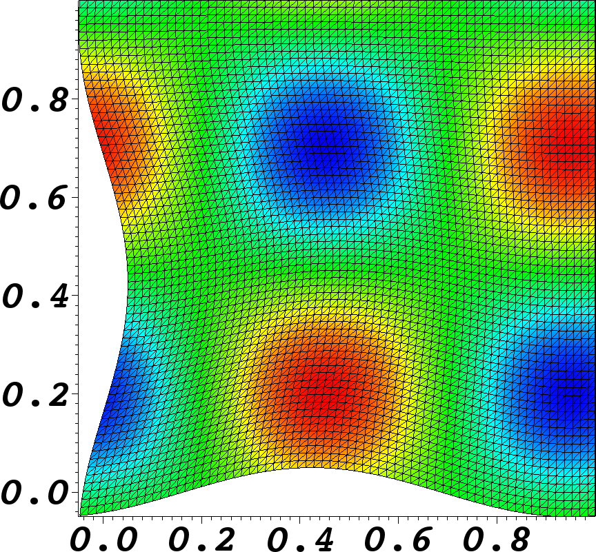
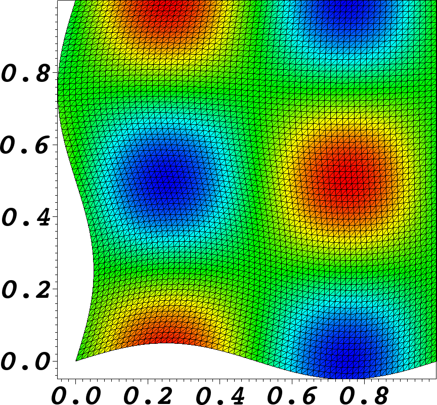
Figure 1: The mesh and pressure solution at different points in time for the test case described in section 5.1. From left to right the mesh and pressure solution at $t=0.2,\ 0.6,\ 1.0$.

We consider the rates of convergence for polynomial degrees $k=2$ and $k=3$ and on a succession of refined space-time meshes. The coarsest space-time mesh consists of $6\cdot 8^{2}$ tetrahedra per space-time slab with $\Delta t=0.05$. For the Picard iteration eq. 24 we set $\text{TOL}=10^{-12}$.

The rates of convergence over the entire space-time domain $\mathcal{E}$, with $\nu=10^{-7}$, are shown in fig. 2. We observe that all space-time methods converge optimally, i.e., the velocity error is of order $\mathcal{O}(h^{k+1})$ and the pressure error is of order $\mathcal{O}(h^{k})$. We observe that the space-time EDG and EHDG methods give smaller errors than the space-time HDG method for the same number of globally coupled degrees-of-freedom.

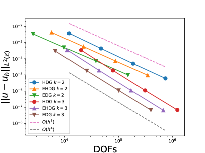
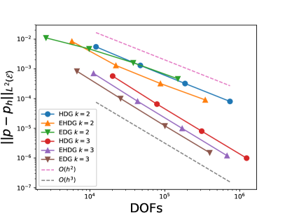
Figure 2: $L^{2}$-norm of the error of the velocity and the pressure on $\mathcal{E}$, with $\nu=10^{-7}$, plotted against the number of globally coupled unknowns.

From Proposition 1 and Remark 1 we know that the error in the divergence of the approximate velocity is of machine precision for all methods, even on deforming domains. However, unlike the space-time HDG and EHDG methods, the space-time EDG method is not divergence-conforming. We, therefore, compute the $L^{2}$-norm of the jump of the normal component of the velocity across facets in the entire space-time domain $\mathcal{E}$ as this is a measure for the lack of mass conservation. Table 2 shows optimal rates of convergence when the kinematic viscosity is $\nu=10^{-4}$. The rates of convergence for the jump of the normal component of the velocity across facets is only sub-optimal for the highly advection-dominated case ($\nu=10^{-7}$).

Cells per slab	Nr. of slabs	$\mathinner{\!\left\lVert\llbracket u_{h}\cdot n\rrbracket\right\rVert}$	rate	$\mathinner{\!\left\lVert\llbracket u_{h}\cdot n\rrbracket\right\rVert}$	rate
$\nu=10^{-4}$		$k=2$		$k=3$
$384$	$20$	2.1e-2	-	1.7e-3	-
$1536$	$40$	4.1e-3	2.3	1.4e-4	3.6
$6144$	$80$	7.0e-4	2.5	9.7e-6	3.8
$24576$	$160$	1.0e-4	2.8	6.6e-7	3.9
$\nu=10^{-7}$		$k=2$		$k=3$
$384$	$20$	2.2e-2	-	1.9e-3	-
$1536$	$40$	4.9e-3	2.2	1.9e-4	3.4
$6144$	$80$	1.0e-3	2.3	1.8e-5	3.4
$24576$	$160$	2.0e-4	2.4	1.6e-6	3.5

Table 2: Rates of convergence for the jump of the normal velocity over facets for the test case describe in section 5.1 using the space-time EDG discretization.

5.2 Flow round a rigid cylinder

We next consider flow round a cylinder [23, 40]. We solve the Navier–Stokes equations on a fixed spatial domain $[0,\ 2.2]\times[0,\ 0.41]$ with flow past a cylindrical obstacle with radius $r=0.05$ centred at $(x_{1},x_{2})=(0.2,0.2)$. We impose a homogeneous Neumann boundary condition on the outflow boundary at $x_{1}=2.2$, while $u=[6x_{2}(0.41-x_{2})/0.41^{2},0]^{T}$ is imposed on the inflow boundary at $x_{1}=0$. On the cylinder and walls $x_{2}=0$ and $x_{2}=0.41$ we impose $u=[0,0]^{T}$. The initial condition is obtained by solving the steady Stokes problem. Finally, we set $\nu=10^{-3}$, $k=3$, $\Delta t=5\cdot 10^{-3}$, $\text{TOL}=10^{-10}$, and use a space-time mesh consisting of $9666$ tetrahedra per slab. The velocity magnitude at final time $t=5$ is shown in fig. 3.

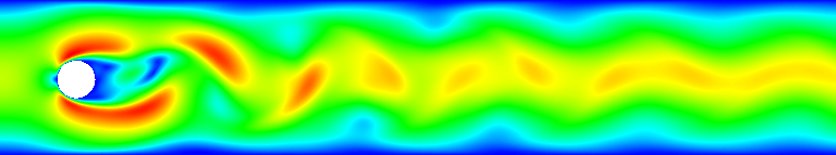
Figure 3: The velocity magnitude of flow around a cylinder, as described in section 5.2, at $t=5$ using $3222$ triangles and $k=3$ and using the space-time EDG method.

Let $\Gamma_{c}$ denote the space-time boundary of the cylinder. We define the lift and drag coefficients as

$$C_{L}=\frac{1}{r\Delta t}\int_{\Gamma_{c}}(\sigma n)\cdot e_{1},\qquad C_{D}=\frac{1}{r\Delta t}\int_{\Gamma_{c}}(\sigma n)\cdot e_{2},$$ (27)

where $\sigma=p\mathbb{I}-\nu\nabla u$, $e_{1}$ and $e_{2}$ are the unit vectors in the $x_{1}$ and $x_{2}$ directions, respectively. Table 3 contains the minimum and maximum $C_{L}$ and $C_{D}$ values computed during the simulations. These values compare well to results found in literature [23, 40].

Table 3 also contains the total number globally coupled degrees-of-freedom for each method. It is clear that even though the space-time EHDG and EDG have less degrees-of-freedom than the space-time HDG method, their output is similar.

Method	$\min C_{L}$	$\max C_{L}$	$\min C_{D}$	$\max C_{D}$	Nr. of unknowns
ST-HDG	-1.014	0.98	3.153	3.219	489840
ST-EHDG	-1.018	0.975	3.153	3.219	268944
ST-EDG	-1.015	0.978	3.155	3.221	158496

Table 3: Comparison of the minimum and the maximum lift and drag coefficients computed using different space-time methods for flow around a rigid cylinder. See section 5.2.

5.3 Flow round a forced oscillating cylinder

In this test case we consider flow round a forced oscillating cylinder [41]. We solve the Navier–Stokes equations on a spatial domain $[-6,\ 20]\times[-6,\ 6]$ with flow past a cylindrical obstacle with radius $r=0.5$ centred initially at $(x_{1},x_{2})=(0,0)$. We prescribe a vertical oscillatory movement of the centre of the cylinder for $t\geq 0$ by

$$x_{2}(t)=0.48\sin(2\pi t/5.94).$$

We apply a homogeneous Neumann boundary condition on the outflow boundary at $x_{1}=20$. On the wall boundaries $x_{1}=-6$, $x_{2}=6$, and $x_{2}=-6$ we impose $u=[1,0]^{T}$, while $u=[0,0]^{T}$ is imposed on the cylinder. The initial condition is obtained by solving the steady Stokes problem and the remaining parameters are chosen as: $\nu=10^{-2}$, $\Delta t=0.025$, $\text{TOL}=10^{-9}$, $k=3$, and the computational domain consists of 20052 tetrahedra per space-time slab.

To accommodate the time-dependent movement of the cylinder, the mesh is updated at each time step as follows. Nodes inside the spatial box $\Omega^{\text{in}}(t)=[-2,\ 2]\times[-2+x_{2}(t),\ 2+x_{2}(t)]$ move with the cylinder while nodes outside the spatial box $\Omega^{\text{out}}=[-4,\ 4]\times[-4,\ 4]$ remain fixed. The movement of the remaining nodes in $\Omega^{\text{out}}\backslash\Omega^{\text{in}}(t)$ decreases linearly with distance. A plot of the mesh when the cylinder is in its highest and lowest position is given in fig. 4.

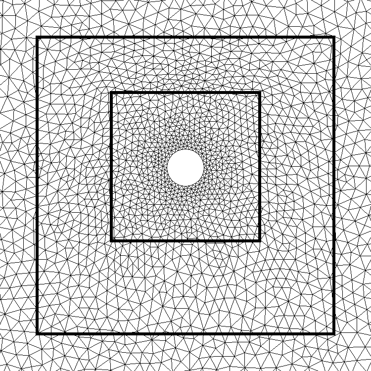
(a) Cylinder at its highest position.

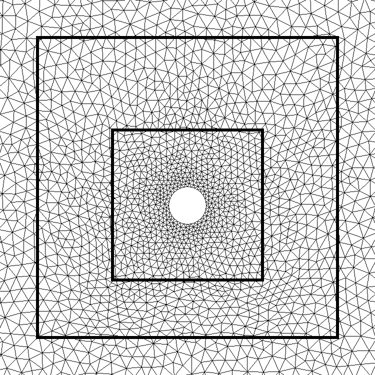
(b) Cylinder at its lowest position.

Figure 4: Mesh deformation during one cycle of the cylinder motion. The small square depicts $\Omega^{\text{in}}(t)$ which moves with the cylinder. The large square depicts $\Omega^{\text{out}}$. See section 5.3.

We plot the lift and drag coefficients as a function of position in fig. 5. We observe periodic behaviour in the lift coefficient, and close to periodic behaviour in the drag coefficient. There is little difference in the solution computed using the space-time EDG and EHDG methods.

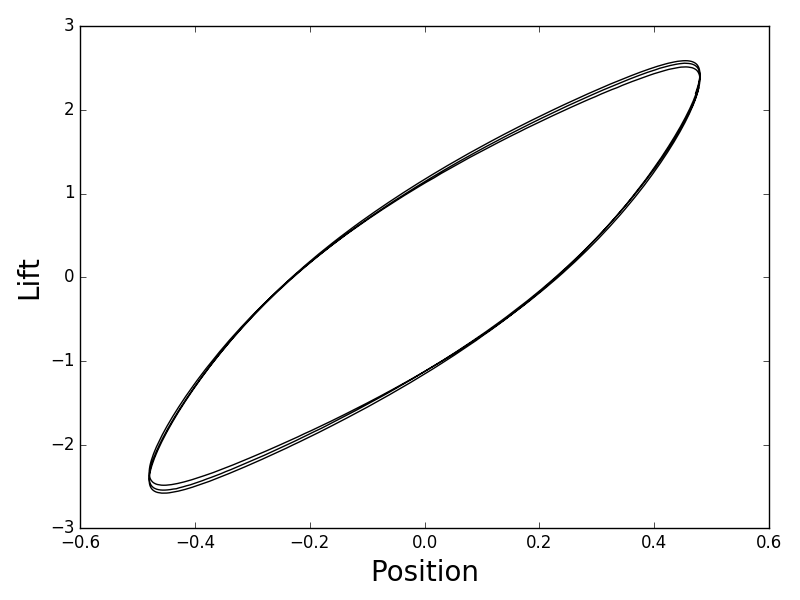
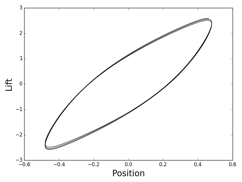
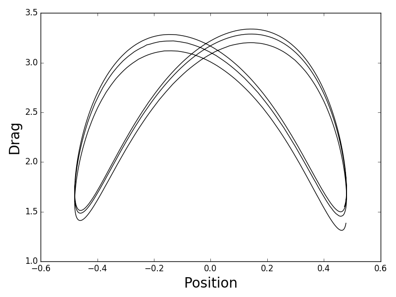
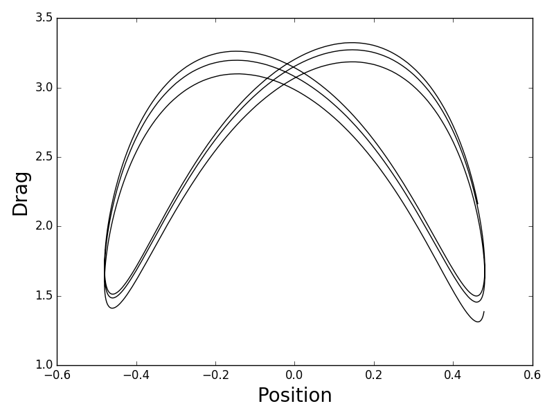
Figure 5: Lift and drag coefficients as a function of the centre of the cylinder, for the test case described in section 5.3. Left: the space-time EDG method. Right: the space-time EHDG method.

The velocity magnitude within one cycle of the cylinder motion computed using the space-time EDG method is shown in fig. 6. We observe that vortices flow downstreem and that the flow field around the cylinder at the end of the cycle is similar to the flow field at the beginning of the cycle. This was observed also in [41].

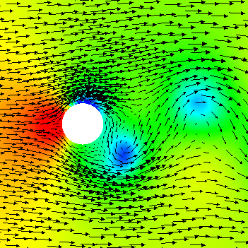
(a) Solution at $t=17.8$.

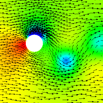
(b) Solution at $t=19.3$.

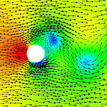
(c) Solution at $t=20.8$.

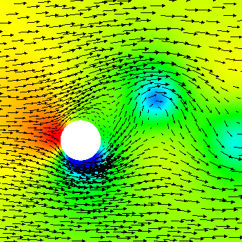
(d) Solution at $t=22.3$.

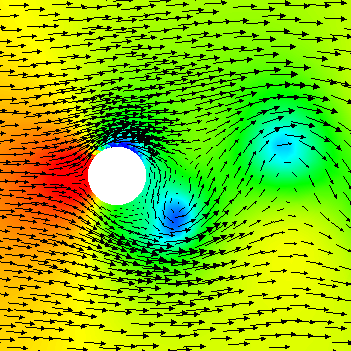
(e) Solution at $t=23.8$.

Figure 6: Velocity vector plot and pressure field around an oscillating cylinder, as described in section 5.3. The plots are at different points in time in one cycle of the cylinder motion.

5.4 Flow past a pitching and plunging NACA0012 airfoil

In this final test case we simulate flow around a pitching and plunging NACA0012 airfoil [7] set in a spatial domain $[-5,\ 10]\times[-5,\ 5]$. The airfoil is initially at $0^{\circ}$ angle of attack with trailing edge at $(x_{1},x_{2})=(-0.5,0.5)$. Throughout the simulation the trailing edge oscillates vertically between $x_{2}=-0.5$ and $x_{2}=0.5$, while the angle of attack changes between $-10^{\circ}$ and $10^{\circ}$. Both of these movements happen with a non-dimensional frequency of $0.5$.

The computational domain consists of 24306 tetrahedra per space-time slab. As parameters we set $k=2$, $\Delta t=0.01$, $\text{TOL}=10^{-7}$, and we set the kinematic viscosity to be $\nu=10^{-3}$.

To account for the time-dependent movement of the airfoil, the mesh is updated at each time step as follows. Nodes within a radius of 1.5 from the trailing edge rotate with the airfoil, nodes outside a radius of 2 from the trailing edge remain fixed. The vertical movement of the nodes is treated similarly as in section 5.3; nodes inside the spatial box $\Omega^{\text{in}}(t)=[-3,\ 7]\times[-3+x_{2}(t),\ 3+x_{2}(t)]$ move with the airfoil, with $x_{2}(t)$ the $x_{2}$ coordinate of the trailing edge, nodes outside the spatial box $\Omega^{\text{out}}=[-4,\ 8]\times[-4.5\,4.5]$ remain fixed, while the movement of the remaining nodes in $\Omega^{\text{out}}\backslash\Omega^{\text{in}}$ decreases linearly with distance. We plot the mesh at different instances in time in fig. 7.

In fig. 8 we plot the pressure and velocity vector fields, computed using the space-time EHDG method, for one cycle of the airfoil motion. When the airfoil is at its highest point, small vortices detach from the airfoil as the airfoil plunges. In fig. 8a we see three small vortices, about a chord length above the airfoil, that detached from the airfoil when it was in its highest position. These small vortices combine into larger vortices downstream. A similar process occurs when the airfoil is at its lowest position, resulting in a street of vortices behind the airfoil. These observations are in agreement with [7].

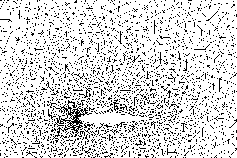
(a) Mesh at start of cycle.

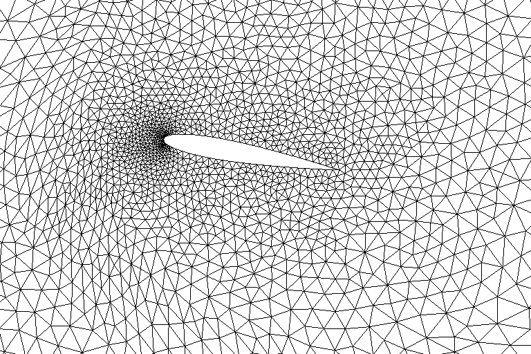
(b) Mesh at quarter of cycle.

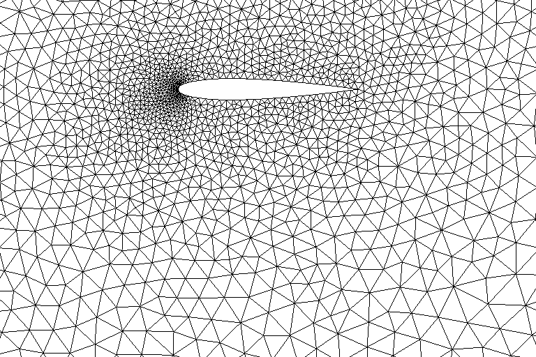
(c) Mesh halfway through cycle.

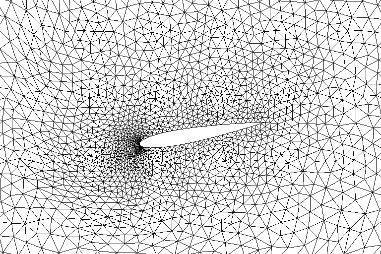
(d) Mesh at three quarters of cycle.

Figure 7: Mesh deformation of the pitching and plunging NACA0012 airfoil during one cycle of motion. See section 5.4.

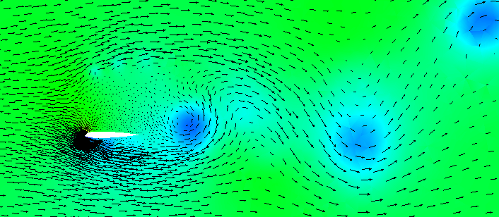
(a) Solution at $t=11$.

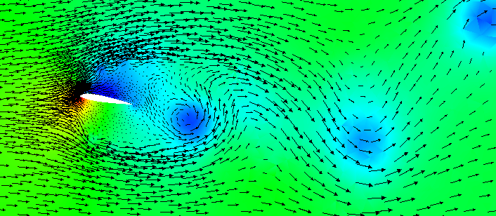
(b) Solution at $t=11.13$.

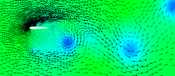
(c) Solution at $t=11.25$.

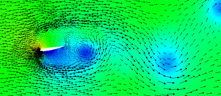
(d) Solution at $t=11.37$.

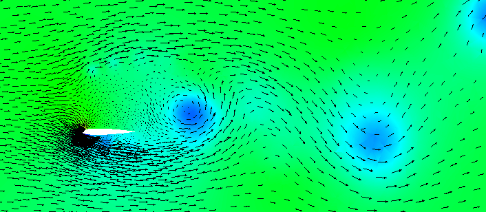
(e) Solution at $t=11.5$.

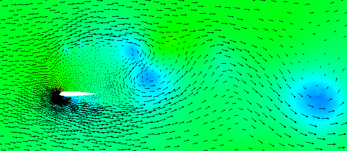
(f) Solution at $t=13$.

Figure 8: Velocity vector plot and pressure field around a pitching and plunging NACA0012 airfoil, see section 5.4. From left to right and top to bottom the first five pictures show the vortices within one cycle of the airfoil motion. The last picture shows the vortices three cycles later.

6 Conclusions

We presented a space-time embedded-hybridized and a space-time embedded discontinuous Galerkin finite element method for the Navier–Stokes equations on moving/deforming domains. Both of these schemes guarantee a point-wise divergence-free velocity field and are shown to be energy-stable, even on time-dependent domains. Although the space-time embedded discontinuous Galerkin method has fewer globally coupled degrees-of-freedom than the space-time embedded-hybridized discontinuous Galerkin method, only the latter discretization conserves mass locally. We have shown the performance of these methods in terms of rates of convergence, and flow simulations around a fixed and a moving cylinder and a pitching and plunging airfoil.

Acknowledgements

SR gratefully acknowledges support from the Natural Sciences and Engineering Research Council of Canada through the Discovery Grant program (RGPIN-05606-2015).

References

- Lesoinne and Farhat [1996] M. Lesoinne, C. Farhat, Geometric conservation laws for flow problems with moving boundaries and deformable meshes, and their impact on aeroelastic computations, Comput. Methods. Appl. Mech. Engrg. 134 (1996) 71–90. doi:10.1016/0045-7825(96)01028-6.
- Guillard and Farhat [2000] H. Guillard, C. Farhat, On the significance of the geometric conservation law for flow computations on moving meshes, Comput. Methods. Appl. Mech. Engrg. 190 (2000) 1467–1482. doi:10.1016/S0045-7825(00)00173-0.
- Ivančić et al. [2019] F. Ivančić, T. W.-H. Sheu, M. Solovchuk, Arbitrary Lagrangian Eulerian-type finite element methods formulation for PDEs on time-dependent domains with vanishing discrete space conservation law, SIAM J. Sci. Comput. 41 (2019) A1548–A1573. doi:10.1137/18M1214494.
- Persson et al. [2009] P.-O. Persson, J. Bonet, J. Peraire, Discontinuous Galerkin solution of the Navier–Stokes equations on deformable domains, Comput. Methods. Appl. Mech. Engrg. 198 (2009) 1585–1595. doi:10.1016/j.cma.2009.01.012.
- Eriksson et al. [1985] K. Eriksson, C. Johnson, V. Thomée, Time discretization of parabolic problems by the discontinuous Galerkin method, RAIRO Modél. Math. Anal. Numér. 19 (1985) 611–643.
- Jamet [1978] P. Jamet, Galerkin-type approximations which are discontinuous in time for parabolic equations in a variable domain, SIAM J. Numer. Anal. 15 (1978) 912–928. doi:10.1137/0715059.
- Johnson and Tezduyar [1994] A. A. Johnson, T. E. Tezduyar, Mesh update strategies in parallel finite element computations of flow problems with moving boundaries and interfaces, Comput. Methods. Appl. Mech. Engrg. 119 (1994) 73–94. doi:10.1016/0045-7825(94)00077-8.
- Masud and Hughes [1997] A. Masud, T. J. R. Hughes, A space-time Galerkin/least-squares finite element formulation of the Navier-Stokes equations for moving domain problems, Comput. Methods. Appl. Mech. Engrg. 146 (1997) 91–126. doi:10.1016/S0045-7825(96)01222-4.
- Tezduyar et al. [1992] T. E. Tezduyar, M. Behr, J. Liou, A new strategy for finite element computations involving moving boundaries and interfaces–the DSD/ST procedure: I. the concept and the preliminary numerical tests, Comput. Methods. Appl. Mech. Engrg. 94 (1992) 339–351. doi:10.1016/0045-7825(92)90059-S.
- N’dri et al. [2001] D. N’dri, A. Garon, A. Fortin, A new stable space–time formulation for two-dimensional and three-dimensional incompressible viscous flow, Int. J. Numer. Meth. Fluids 37 (2001) 865–884. doi:10.1002/fld.174.
- N’dri et al. [2002] D. N’dri, A. Garon, A. Fortin, Incompressible Navier–Stokes computations with stable and stabilized space–time formulations: a comparative study, Commun. Numer. Meth. Engng. 18 (2002) 495–512. doi:10.1002/cnm.507.
- van der Vegt and van der Ven [2002] J. J. W. van der Vegt, H. van der Ven, Space–time discontinuous Galerkin finite element method with dynamic grid motion for inviscid compressible flow, J. Comput. Phys. 182 (2002) 546–585. doi:10.1006/jcph.2002.7185.
- Rhebergen et al. [2013] S. Rhebergen, B. Cockburn, J. van der Vegt, A space–time discontinuous Galerkin method for the incompressible Navier–Stokes equations, J. Comput. Phys. 233 (2013) 339–358. doi:10.1016/j.jcp.2012.08.052.
- van der Vegt and Sudirham [2008] J. van der Vegt, J. Sudirham, A space–time discontinuous Galerkin method for the time-dependent Oseen equations, Appl. Numer. Math 58 (2008) 1892–1917. doi:10.1016/j.apnum.2007.11.010.
- Rhebergen and Cockburn [2012] S. Rhebergen, B. Cockburn, A space-time hybridizable discontinuous Galerkin method for incompressible flows on deforming domains, J. Comput. Phys. 231 (2012) 4185–4204. doi:10.1016/j.jcp.2012.02.011.
- Rhebergen and Cockburn [2013] S. Rhebergen, B. Cockburn, Space–time hybridizable discontinuous Galerkin method for the advection–diffusion equation on moving and deforming meshes, in: C. de Moura, C. Kubrusly (Eds.), The Courant–Friedrichs–Lewy (CFL) condition, 80 years after its discovery, Birkhäuser Science, 2013, pp. 45–63. doi:10.1007/978-0-8176-8394-8_4.
- Kirk et al. [2019] K. L. A. Kirk, T. L. Horvath, A. Cesmelioglu, S. Rhebergen, Analysis of a space–time hybridizable discontinuous Galerkin method for the advection–diffusion problem on time-dependent domains, SIAM J. Numer. Anal. 57 (2019) 1677–1696. doi:10.1137/18M1202049.
- Cockburn et al. [2009] B. Cockburn, J. Gopalakrishnan, R. Lazarov, Unified hybridization of discontinuous Galerkin, mixed, and continuous Galerkin methods for second order elliptic problems, SIAM J. Numer. Anal. 47 (2009) 1319–1365. doi:10.1137/070706616.
- Nguyen and Peraire [2012] N. C. Nguyen, J. Peraire, Hybridizable discontinuous Galerkin methods for partial differential equations in continuum mechanics, J. Comput. Phys. 231 (2012) 5955–5988. doi:10.1016/j.jcp.2012.02.033.
- Cesmelioglu et al. [2017] A. Cesmelioglu, B. Cockburn, W. Qiu, Analysis of a hybridizable discontinuous Galerkin method for the steady-state incompressible Navier–Stokes equations, Math. Comp. 86 (2017) 1643–1670. doi:10.1090/mcom/3195.
- Fu [2019] G. Fu, An explicit divergence-free DG method for incompressible flow, Comput. Methods Appl. Mech. Engrg. 345 (2019) 502–517. URL: https://doi.org/10.1016/j.cma.2018.11.012.
- Labeur and Wells [2012] R. J. Labeur, G. N. Wells, Energy stable and momentum conserving hybrid finite element method for the incompressible Navier–Stokes equations, SIAM J. Sci. Comput. 34 (2012) A889–A913. doi:10.1137/100818583.
- Lehrenfeld and Schöberl [2016] C. Lehrenfeld, J. Schöberl, High order exactly divergence-free hybrid discontinuous Galerkin methods for unsteady incompressible flows, Comput. Methods Appl. Mech. Engrg. 307 (2016) 339–361. doi:10.1016/j.cma.2016.04.025.
- Nguyen et al. [2011] N. C. Nguyen, J. Peraire, B. Cockburn, An implicit high–order hybridizable discontinuous Galerkin method for the incompressible Navier–Stokes equations, J. Comput. Phys. 230 (2011) 1147–1170. doi:10.1016/j.jcp.2010.10.032.
- Qiu and Shi [2016] W. Qiu, K. Shi, A superconvergent HDG method for the incompressible Navier–Stokes equations on general polyhedral meshes, IMA J. Numer. Anal. 36 (2016) 1943–1967. URL: http://dx.doi.org/10.1093/imanum/drv067.
- Rhebergen and Wells [2017] S. Rhebergen, G. N. Wells, Analysis of a hybridized/interface stabilized finite element method for the Stokes equations, SIAM J. Numer. Anal. 55 (2017) 1982–2003. doi:10.1137/16M1083839.
- Rhebergen and Wells [2018] S. Rhebergen, G. N. Wells, A hybridizable discontinuous Galerkin method for the Navier–Stokes equations with pointwise divergence-free velocity field, J. Sci. Comput. (2018). doi:10.1007/s10915-018-0671-4.
- Schroeder and Lube [2018] P. Schroeder, G. Lube, Divergence-free H(div)-fem for time-dependent incompressible flows with applications to high Reynolds number vortex dynamics, J. Sci. Comput. 75 (2018) 830–858. URL: https://doi.org/10.1007/s10915-017-0561-1.
- Horvath and Rhebergen [2019] T. L. Horvath, S. Rhebergen, A locally conservative and energy-stable finite element method for the Navier-Stokes problem on time-dependent domains, Int. J. Numer. Meth. Fluids 89 (2019) 519–532. doi:10.1002/fld.4707.
- Rhebergen and Wells [2019] S. Rhebergen, G. N. Wells, An embedded-hybridized discontinuous Galerkin finite element method for the Stokes equations, Comput. Methods Appl. Mech. Engrg. (2019). URL: https://arxiv.org/abs/1811.09194, to appear.
- Cesmelioglu et al. [2019] A. Cesmelioglu, S. Rhebergen, G. N. Wells, An embedded-hybridized discontinuous galerkin method for the coupled stokes-darcy system (2019). URL: https://arxiv.org/abs/1905.09753, submitted.
- van der Ven [2008] H. van der Ven, An adaptive multitime multigrid algorithm for time-periodic flow simulations, J. Comput. Phys. 227 (2008) 5286–5303. doi:10.1016/j.jcp.2008.01.039.
- Wells [2011] G. N. Wells, Analysis of an interface stabilized finite element method: the advection-diffusion-reaction equation, SIAM J. Numer. Anal. 49 (2011) 87–109. doi:10.1137/090775464.
- Dobrev et al. [2018] V. A. Dobrev, T. V. Kolev, et al., MFEM: Modular finite element methods, http://mfem.org, 2018.
- Amestoy et al. [2001] P. Amestoy, I. Duff, J.-Y. L’Excellent, J. Koster, A fully asynchronous multifrontal solver using distributed dynamic scheduling, SIAM J. Matrix Anal. & Appl. 23 (2001) 15–41. doi:10.1137/S0895479899358194.
- Amestoy et al. [2006] P. R. Amestoy, A. Guermouche, J.-Y. L’Excellent, S. Pralet, Hybrid scheduling for the parallel solution of linear systems, Parallel Comput. 32 (2006) 136–156. doi:10.1016/j.parco.2005.07.004.
- Balay et al. [2016a] S. Balay, S. Abhyankar, M. F. Adams, J. Brown, P. Brune, K. Buschelman, L. Dalcin, V. Eijkhout, W. D. Gropp, D. Kaushik, M. G. Knepley, L. Curfman McInnes, K. Rupp, B. F. Smith, S. Zampini, H. Zhang, H. Zhang, PETSc Web page, http://www.mcs.anl.gov/petsc, 2016a.
- Balay et al. [2016b] S. Balay, S. Abhyankar, M. F. Adams, J. Brown, P. Brune, K. Buschelman, L. Dalcin, V. Eijkhout, W. D. Gropp, D. Kaushik, M. G. Knepley, L. Curfman McInnes, K. Rupp, B. F. Smith, S. Zampini, H. Zhang, H. Zhang, PETSc Users Manual, Technical Report ANL-95/11 - Revision 3.7, Argonne National Laboratory, 2016b. URL: http://www.mcs.anl.gov/petsc.
- Balay et al. [1997] S. Balay, W. D. Gropp, L. Curfman McInnes, B. F. Smith, Efficient management of parallelism in object oriented numerical software libraries, in: E. Arge, A. M. Bruaset, H. P. Langtangen (Eds.), Modern Software Tools in Scientific Computing, , Birkhäuser Press, 1997, pp. 163–202.
- Schäfer et al. [1996] M. Schäfer, S. Turek, F. Durst, E. Krause, R. Rannacher, Benchmark computations of laminar flow around a cylinder, in: E. H. Hirschel (Ed.), Flow Simulation with High-Performance Computers II, 1996, pp. 547–566.
- Calderer and Masud [2010] R. Calderer, A. Masud, A multiscale stabilized ALE formulation for incompressible flows with moving boundaries, Comput. Mech. 46 (2010) 185–197. doi:10.1007/s00466-010-0487-z.