Robust Learning Rate Selection
for Stochastic Optimization via Splitting Diagnostic

Abstract

This paper proposes SplitSGD, a new dynamic learning rate schedule for stochastic optimization. This method decreases the learning rate for better adaptation to the local geometry of the objective function whenever a stationary phase is detected, that is, the iterates are likely to bounce at around a vicinity of a local minimum. The detection is performed by splitting the single thread into two and using the inner product of the gradients from the two threads as a measure of stationarity. Owing to this simple yet provably valid stationarity detection, SplitSGD is easy-to-implement and essentially does not incur additional computational cost than standard SGD. Through a series of extensive experiments, we show that this method is appropriate for both convex problems and training (non-convex) neural networks, with performance compared favorably to other stochastic optimization methods. Importantly, this method is observed to be very robust with a set of default parameters for a wide range of problems and, moreover, yields better generalization performance than other adaptive gradient methods such as Adam.

1 Introduction

Many machine learning problems boil down to finding a minimizer $\theta^{*}\in\mathbb{R}^{d}$ of a risk function taking the form

$$F(\theta)=\operatorname{\mathbb{E}}\left[f(\theta,Z)\right],$$ (1.1)

where $f$ denotes a loss function, $\theta$ is the model parameter, and the random data point $Z=(X,y)$ contains a feature vector $X$ and its label $y$. In the case of a finite population, for example, this problem is reduced to the empirical minimization problem. The touchstone method for minimizing (1.1) is stochastic gradient descent (SGD). Starting from an initial point $\theta_{0}$, SGD updates the iterates according to

$${}\theta_{t+1}=\theta_{t}-\eta_{t}\cdot g(\theta_{t},Z_{t+1})$$ (1.2)

for $t\geq 0$, where $\eta_{t}$ is the learning rate, $\{Z_{t}\}_{t=1}^{\infty}$ are i.i.d. copies of $Z$ and $g(\theta,Z)$ is the (sub-) gradient of $f(\theta,Z)$ with respect to $\theta$. The noisy gradient $g(\theta,Z)$ is an unbiased estimate for the true gradient $\nabla F(\theta)$ in the sense that $\operatorname{\mathbb{E}}\left[g(\theta,Z)\right]=\nabla F(\theta)$ for any $\theta$.

The convergence rate of SGD crucially depends on the learning rate—often recognized as “the single most important hyper-parameter” in training deep neural networks (Bengio,, 2012)—and, accordingly, there is a vast literature on how to decrease this fundamental tuning parameter for improved convergence performance. In the pioneering work of Robbins and Monro, (1951), the learning rate $\eta_{t}$ is set to $O(1/t)$ for convex objectives. Later, it was recognized that a slowly decreasing learning rate in conjunction with iterate averaging leads to a faster rate of convergence for strongly convex and smooth objectives (Ruppert,, 1988; Polyak and Juditsky,, 1992). More recently, extensive effort has been devoted to incorporating preconditioning into learning rate selection rules (Duchi et al.,, 2011; Dauphin et al.,, 2015; Tan et al.,, 2016). Among numerous proposals, a simple yet widely employed approach is to repeatedly halve the learning rate after performing a pre-determined number of iterations (see, for example, Bottou et al.,, 2018).

In this paper, we introduce a new variant of SGD that we term SplitSGD with a novel learning rate selection rule. At a high level, our new method is motivated by the following fact: an optimal learning rate should be adaptive to the informativeness of the noisy gradient $g(\theta_{t},Z_{t+1})$. Roughly speaking, the informativeness is higher if the true gradient $\nabla F(\theta_{t})$ is relatively large compared with the noise $\nabla F(\theta_{t})-g(\theta_{t},Z_{t+1})$ and vice versa. On the one hand, if the learning rate is too small with respect to the informativeness of the noisy gradient, SGD makes rather slow progress. On the other hand, the iterates would bounce around a region of an optimum of the objective if the learning rate is too large with respect to the informativeness. The latter case corresponds to a stationary phase in stochastic optimization (Murata,, 1998; Chee and Toulis,, 2018), which necessitates the reduction of the learning rate for better convergence.

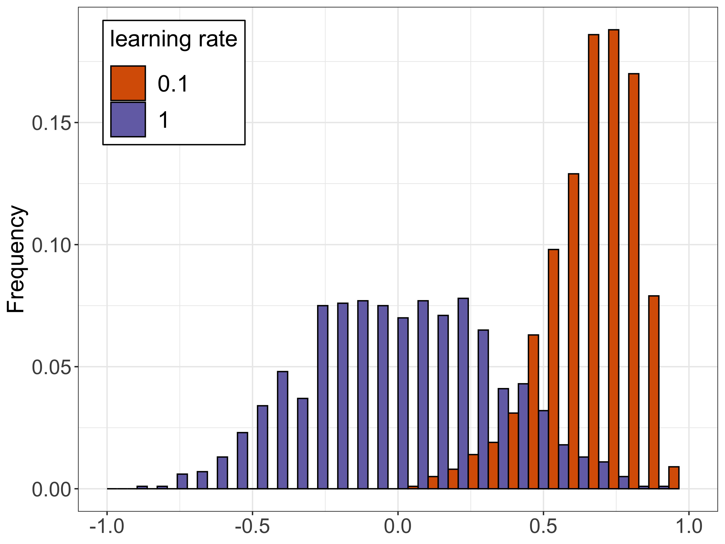
Figure 1: Normalized dot product of averaged noisy gradients over $100$ iterations. Stationarity depends on the learning rate: $\eta=1$ corresponds to stationarity, while $\eta=0.1$ corresponds to non stationarity. Details in Section 2.

SplitSGD differs from other stochastic optimization procedures in its robust stationarity phase detection, which we refer to as the Splitting Diagnostic. In short, this diagnostic runs two SGD threads initialized at the same iterate using independent data points (refers to $Z_{t+1}$ in (1.2)), and then performs hypothesis testing to determine whether the learning rate leads to a stationary phase or not. The effectiveness of the Splitting Diagnostic is illustrated in Figure 1, which reveals different patterns of dependence between the two SGD threads with difference learning rates. Loosely speaking, in the stationary phase (in purple), the two SGD threads behave as if they are independent due to a large learning rate, and SplitSGD subsequently decreases the learning rate by some factor. In contrast, strong positive dependence is exhibited in the non stationary phase (in orange) and, thus, the learning rate remains the same after the diagnostic. In essence, the robustness of the Splitting Diagnostic is attributed to its adaptivity to the local geometry of the objective, thereby making SplitSGD a tuning-insensitive method for stochastic optimization. Its strength is confirmed by our experimental results in both convex and non-convex settings. In the latter, SplitSGD showed robustness with respect to the choice of the initial learning rate, and remarkable success in improving the test accuracy and avoiding overfitting compared to classic optimization procedures.

1.1 Related work

There is a long history of detecting stationarity or non-stationarity in stochastic optimization to improve convergence rates (Yin,, 1989; Pflug,, 1990; Delyon and Juditsky,, 1993; Murata,, 1998; Le Roux et al.,, 2013). Perhaps the most relevant work in this vein to the present paper is Chee and Toulis, (2018), which builds on top of Pflug, (1990) for general convex functions. Specifically, this work uses the running sum of the inner products of successive stochastic gradients for stationarity detection. However, this approach does not take into account the strong correlation between consecutive gradients and, moreover, is not sensitive to the local curvature of the current iterates due to unwanted influence from prior gradients. In contrast, the splitting strategy, which is akin to HiGrad (Su and Zhu,, 2018), allows our SplitSGD to concentrate on the current gradients and leverage the regained independence of gradients to test stationarity. Lately, Yaida, (2019) and Lang et al., (2019) derive a stationarity detection rule that is based on gradients of a mini-batch to tune the learning rate in SGD with momentum.

From a different angle, another related line of work is concerned with the relationship between the informativeness of gradients and the mini-batch size (Keskar et al.,, 2016; Yin et al.,, 2017; Li et al.,, 2017; Smith et al.,, 2017). Among others, it has been recognized that the optimal mini-batch size should be adaptive to the local geometry of the objective function and the noise level of the gradients, delivering a growing line of work that leverage the mini-batch gradient variance for learning rate selection (Byrd et al.,, 2012; Balles et al.,, 2016; Balles and Hennig,, 2017; De et al.,, 2017; Zhang and Mitliagkas,, 2017; McCandlish et al.,, 2018).

2 The SplitSGD algorithm

In this section, we first develop the Splitting Diagnostic for stationarity detection, followed by the introduction of the SplitSGD algorithm in detail.

Figure 2: The architecture of SplitSGD. The initial learning rate is $\eta$ and the length of the first single thread is $t_{1}$. If the diagnostic does not detect stationarity, the length and learning rate of the next thread remain unchanged. If stationarity is observed, we decrease the learning rate by a factor $\gamma$ and proportionally increase the length.

2.1 Diagnostic via Splitting

Intuitively, the stationarity phase occurs when two independent threads with the same starting point are no longer moving along the same direction. This intuition is the motivation for our Splitting Diagnostic, which is presented in Algorithm 2 and described in what follows. We call $\theta_{0}$ the initial value, even though later it will often have a different subscript based on the number of iterations already computed before starting the diagnostic. From the starting point, we run two SGD threads, each consisting of $w$ windows of length $l$. For each thread $k=1,2$, we define $g_{t}^{(k)}=g(\theta_{t}^{(k)},Z_{t+1}^{(k)})$ and the iterates are

$$\theta_{t+1}^{(k)}=\theta_{t}^{(k)}-\eta\cdot g_{t}^{(k)},$$ (2.1)

where $t\in\{0,...,wl-1\}$. On every thread we compute the average noisy gradient in each window, indexed by $i=1,...,w$, which is

$$\bar{g}_{i}^{(k)}:=\frac{1}{l}\sum_{j=1}^{l}g_{(i-1)\cdot l+j}^{(k)}=\frac{\theta_{(i-1)\cdot l+1}^{(k)}-\theta_{i\cdot l}^{(k)}}{l\cdot\eta}.$$ (2.2)

The length $l$ of each window has the same function as the mini-batch parameter in mini-batch SGD (Li et al.,, 2014), in the sense that a larger value of $l$ aims to capture more of the true signal by averaging out the errors. At the end of the diagnostic, we have stored two vectors, each containing the average noisy gradients in the windows in each thread.

Definition 2.1.

For $i=1,...,w$, we define the gradient coherence with respect to the starting point of the Splitting Diagnostic $\theta_{0}$, the learning rate $\eta$, and the length of each window $l$, as

$${}Q_{i}(\theta_{0},\eta,l)=\langle\bar{g}_{i}^{(1)},\bar{g}_{i}^{(2)}\rangle.$$ (2.3)

We will drop the dependence from the parameters and refer to it simply as $Q_{i}$.

The gradient coherence expresses the relative position of the average noisy gradients, and its sign indicates whether the SGD updates have reached stationarity. In fact, if in the two threads the noisy gradients are pointing on average in the same direction, it means that the signal is stronger than the noise, and the dynamic is still in its transient phase. On the contrary, when the gradient coherence is on average very close to zero, and it also assumes negative values thanks to its stochasticity, this indicates that the noise component in the gradient is now dominant, and stationarity has been reached. Of course these values, no matter how large $l$ is, are subject to some randomness. Our diagnostic then considers the signs of $Q_{1},...,Q_{w}$ and returns a result based on the proportion of negative $Q_{i}$. One output is a boolean value $T_{D}$, defined as follows:

$${}T_{D}=\left\{\begin{array}[]{ll}S&\text{if}\quad\sum_{i=1}^{w}(1-\operatorname{sign}{(Q_{i})})/2\geq q\cdot w\\[5.0pt] N&\text{if}\quad\sum_{i=1}^{w}(1-\operatorname{sign}{(Q_{i})})/2<q\cdot w.\end{array}\right.$$ (2.4)

where $T_{D}=S$ indicates that stationarity has been detected, and $T_{D}=N$ means non-stationarity. The parameter $q\in[0,1]$ controls the tightness of this guarantee, being the smallest proportion of negative $Q_{i}$ required to declare stationarity. In addition to $T_{D}$, we also return the average last iterate of the two threads as a starting point for following iterations. We call it $\theta_{D}:=(\theta_{w\cdot l}^{(1)}+\theta_{w\cdot l}^{(2)})/2.$

Algorithm 1 Diagnostic($\eta,w,l,q,\theta^{in}$)

1:  $\theta_{0}^{(1)}=\theta_{0}^{(2)}=\theta^{in}$

2:  for $i=1,...,w$ do

3:     for $k=1,2$ do

4:        for $j=0,...,l-1$ do

5:           $\theta_{(i-1)\cdot l+j+1}^{(k)}=\theta_{(i-1)\cdot l+j}^{(k)}-\eta\cdot g_{(i-1)\cdot l+j}^{(k)}$

6:        end for

7:        $\bar{g}_{i}^{(k)}=(\theta_{(i-1)\cdot l+1}^{(k)}-\theta_{i\cdot l}^{(k)})/l\cdot\eta$.

8:     end for

9:     $Q_{i}=\langle\bar{g}_{i}^{(1)},\bar{g}_{i}^{(2)}\rangle$

10:  end for

11:  if $\sum_{i=1}^{w}(1-\operatorname{sign}{(Q_{i})})/2\geq q\cdot w$ then

12:     return  $\left\{\theta_{D}=(\theta_{w\cdot l}^{(1)}+\theta_{w\cdot l}^{(2)})/2,\ T_{D}=S\right\}$

13:  else

14:     return  $\left\{\theta_{D}=(\theta_{w\cdot l}^{(1)}+\theta_{w\cdot l}^{(2)})/2,\ T_{D}=N\right\}$

15:  end if

2.2 The Algorithm

The Splitting Diagnostic can be employed in a more sophisticated SGD procedure, which we call SplitSGD. We start by running the standard SGD with constant learning rate $\eta$ for $t_{1}$ iterations. Then, starting from $\theta_{t_{1}}$, we use the Splitting Diagnostic to verify if stationarity has been reached. If stationarity is not detected, the next single thread has the same length $t_{1}$ and learning rate $\eta$ as the previous one. On the contrary, if $T_{D}=S$, we decrease the learning rate by a factor $\gamma\in(0,1)$ and increase the length of the thread by $1/\gamma$, as suggested by Bottou et al., (2018) in their SGD^1/2 procedure. Notice that, if $q=0$, then the learning rate gets deterministically decreased after each diagnostic. On the other extreme, if we set $q=1$, then the procedure maintains constant learning rate with high probability. Figure 2 illustrates what happens when the first diagnostic does not detect stationarity, but the second one does. SplitSGD puts together two crucial aspects: it employs the Splitting Diagnostic at deterministic times, but it does not deterministically decreases the learning rate. We will see in Section 4 how both of these features come into play in the comparison with other existing methods. A detailed explanation of SplitSGD is presented in Algorithm 2.

Algorithm 2 SplitSGD($\eta,w,l,q,B,t_{1},\theta_{0},\gamma$)

1:  $\eta_{1}=\eta$

2:  $\theta_{1}^{in}=\theta_{0}$

3:  for $b=1,...,B$ do

4:     Run SGD with constant step size $\eta_{b}$ for $t_{b}$ steps, starting from $\theta_{b}^{in}$

5:     Let the last update be $\theta_{b}^{last}$

6:     $D_{b}=\textbf{Diagnostic}(\eta_{b},w,l,q,\theta_{b}^{last})$

7:     $\theta_{b+1}^{in}=\theta_{D_{b}}$

8:     if $T_{D_{b}}=S$ then

9:        $\eta_{b+1}=\gamma\cdot\eta_{b}$ and $t_{b+1}=\lfloor t_{b}/\gamma\rfloor$

10:     else

11:        $\eta_{b+1}=\eta_{b}$ and $t_{b+1}=t_{b}$

12:     end if

13:  end for

3 Theoretical Guarantees for Stationarity Detection

This section develops theoretical guarantees for the validity of our learning rate selection. Specifically, in the case of a relatively small learning rate, we can imagine that, if the number of iterations is fixed, the SGD updates are not too far from the starting point, so the stationary phase has not been reached yet. On the other hand, however, when $t\to\infty$ and the learning rate is fixed, we would like the diagnostic to tell us that we have reached stationarity, since we know that in this case the updates will oscillate around $\theta^{*}$. Our first assumption concerns the convexity of the function $F(\theta)$. It will not be used in Theorem 1, in which we focus our attention on a neighborhood of $\theta_{0}$.

Assumption 3.1.

The function $F$ is strongly convex, with convexity constant $\mu>0$. For all $\theta_{1},\theta_{2}$,

$$F(\theta_{1})\geq F(\theta_{2})+\langle\nabla F(\theta_{2}),\theta_{1}-\theta_{2}\rangle+\frac{\mu}{2}\|\theta_{1}-\theta_{2}\|^{2}$$

and also $\|\nabla F(\theta_{1})-\nabla F(\theta_{2})\|\geq\mu\cdot\|\theta_{1}-\theta_{2}\|.$

Assumption 3.2.

The function $F$ is smooth, with smoothness parameter $L>0$. For all $\theta_{1},\theta_{2}$,

$$\|\nabla F(\theta_{1})-\nabla F(\theta_{2})\|\leq L\cdot\|\theta_{1}-\theta_{2}\|.$$

We said before that the noisy gradient is an unbiased estimate of the true gradient. The next assumption that we make is on the distribution of the errors.

Assumption 3.3.

We define the error in the evaluation of the gradient in $\theta_{t-1}$ as

$$\epsilon_{t}:=\epsilon(\theta_{t-1},Z_{t})=g(\theta_{t-1},Z_{t})-\nabla F(\theta_{t-1})$$ (3.1)

and the filtration $\mathcal{F}_{t}=\sigma(Z_{1},...,Z_{t})$. Then $\epsilon_{t}\in\mathcal{F}_{t}$ and $\{\epsilon_{t}\}_{t=1}^{\infty}$ is a martingale difference sequence with respect to $\{\mathcal{F}_{t}\}_{t=1}^{\infty}$, which means that $\operatorname{\mathbb{E}}[\epsilon_{t}|\mathcal{F}_{t-1}]=0.$ The covariance of the errors satisfies

$${}\sigma_{\min}\cdot I\preceq\operatorname{\mathbb{E}}\left[\epsilon_{t}\epsilon_{t}^{T}\ |\ \mathcal{F}_{t-1}\right]\preceq\sigma_{\max}\cdot I,$$ (3.2)

where $0<\sigma_{\min}\leq\sigma_{\max}<\infty$ for any $\theta$.

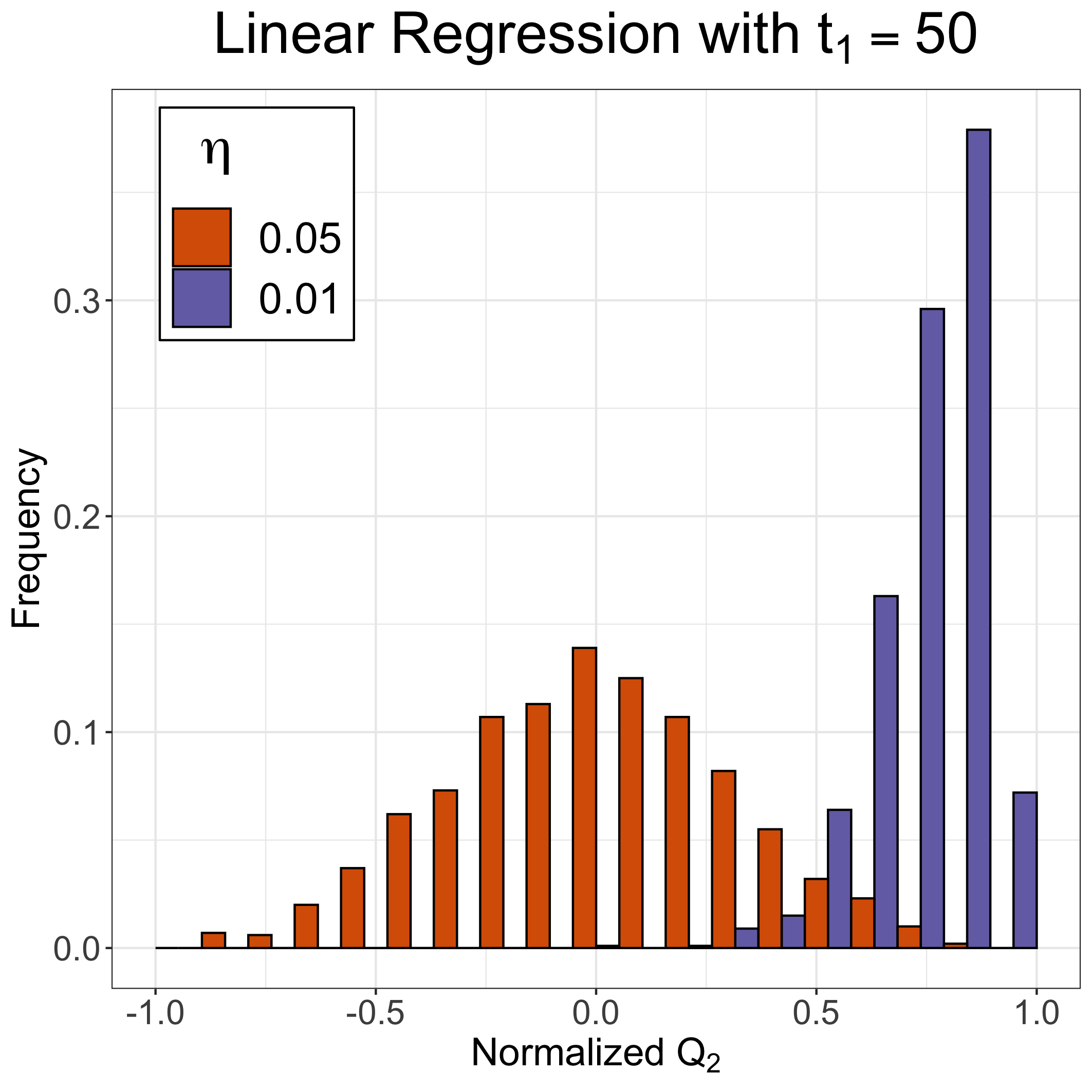
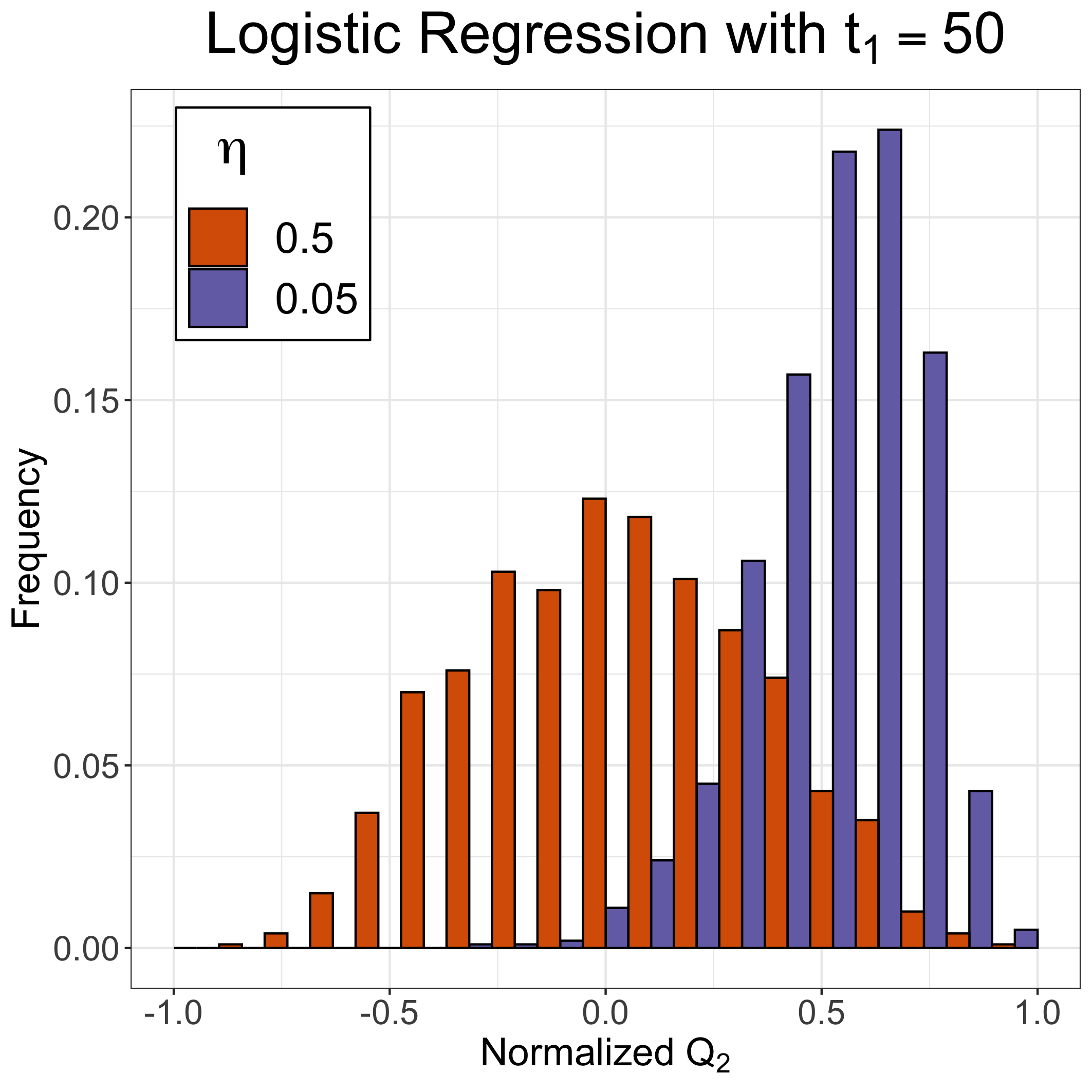
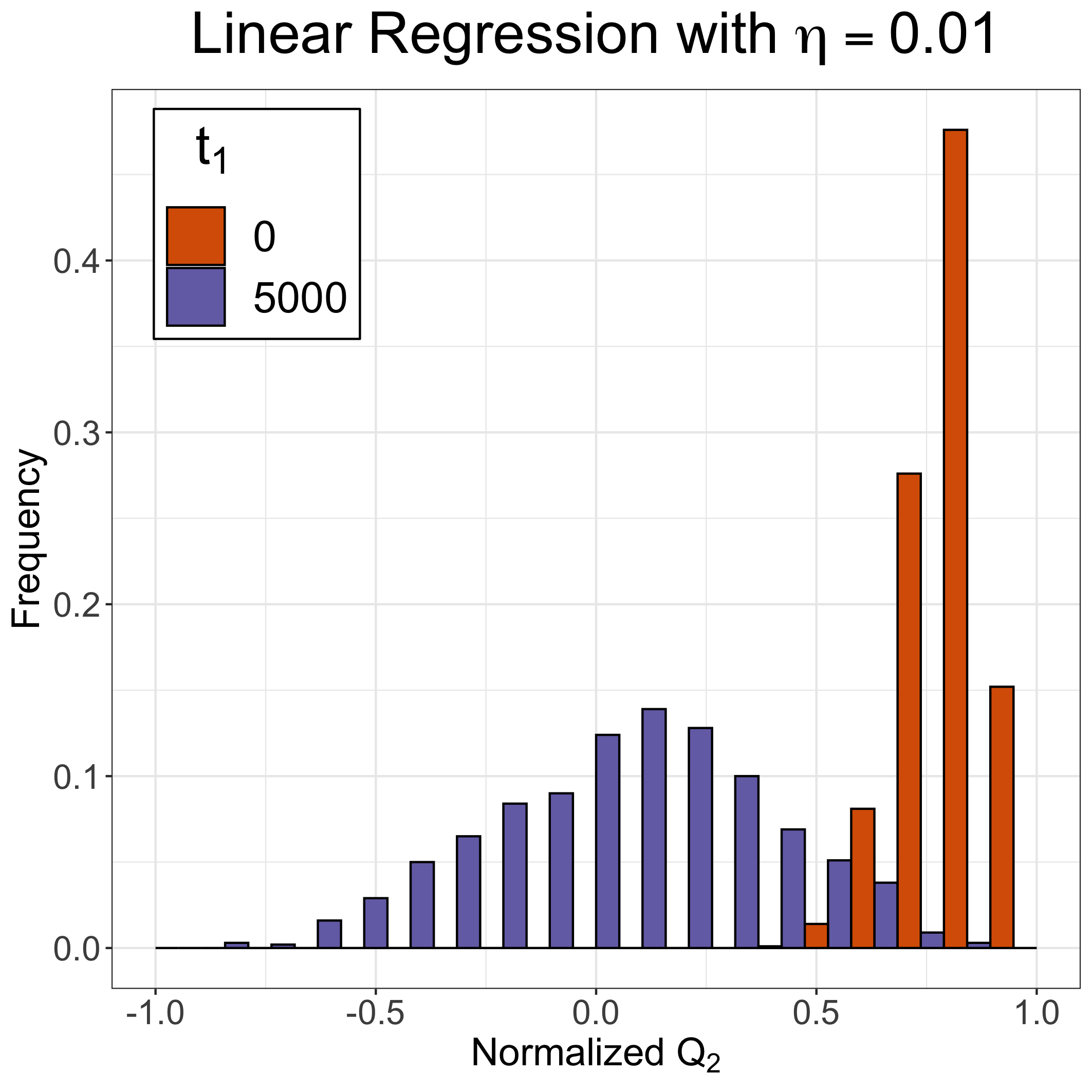
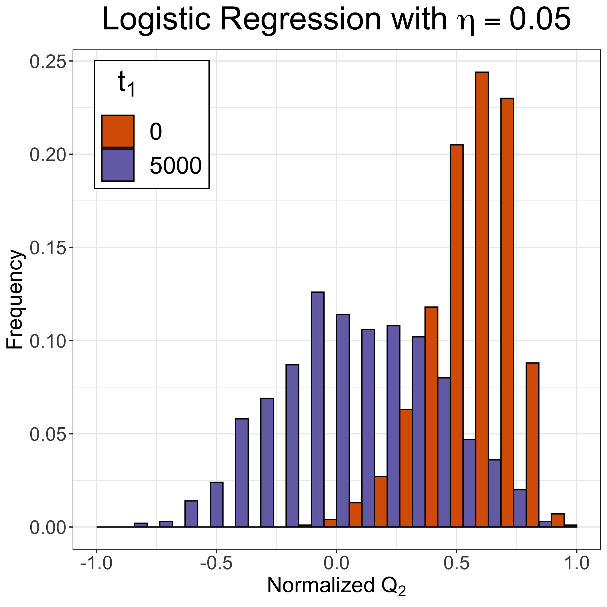
Figure 3: Histogram of the gradient coherence $Q_{i}$ (here for the second pair of windows, and normalized) of the Splitting Diagnostic for linear and logistic regression. The two top panels show the behavior described in Theorem 1, the two bottom panels the one in Theorem 2.

Our last assumption is on the noisy functions $f(\theta,Z)$ and on an upper bound on the moments of their gradient. We do not specify $m$ here since different values are used in the next two theorems.

Assumption 3.4.

Each function $f(\theta,Z)$ is convex, and there exists a constant $G$ such that $\operatorname{\mathbb{E}}\left[\|g(\theta_{t},Z_{t+1})\|^{m}\ |\ \mathcal{F}_{t}\right]\leq G^{m}$ for any $\theta_{t}$.

We first show that there exists a learning rate sufficiently small such that the standard deviation of any gradient coherence $Q_{i}$ is arbitrarily small compared to its expectation, and the expectation is positive because $\theta_{t_{1}+l}$ is not very far from $\theta_{0}$. This implies that the probability of any gradient coherence to be negative, $\operatorname{\mathbb{P}}(Q_{i}<0)$, is extremely small, which means that the Splitting Diagnostic will return $T_{D}=N$ with high probability.

Theorem 1.

If Assumptions 3.2, 3.3 and 3.4 with $m=4$ hold, and we run $t_{1}$ iterations before the Splitting Diagnostic, then for any $i\in\{1,...,w\}$ we can set $\eta$ small enough to guarantee that

$$\operatorname{sd}(Q_{i})\leq C_{1}(\eta,l)\cdot\operatorname{\mathbb{E}}\left[Q_{i}\right],$$

where $C_{1}(\eta,l)=O(1/\sqrt{l})+O(\sqrt{\eta(t_{1}+l)})$. Proof in Appendix B.

In the two left panels of Figure 3 we provide a visual interpretation of this result. When $\eta$ is sufficiently small all the mass of the distribution of $Q_{i}$ is concentrated on positive values. Note that to obtain this result we do not need to use the strong convexity Assumption 3.1 since, when $\eta(t_{1}+l)$ is small, $\theta_{t_{1}+l}$ is not very far from $\theta_{0}$. In the next Theorem we show that, if we let the SGD thread before the diagnostic run for long enough and the learning rate is not too big, then the splitting diagnostic output is $T_{D}=S$ probability that can be made arbitrarily high. This is consistent with the fact that, as $t_{1}\to\infty$, the iterates will start oscillating in a neighborhood of $\theta^{*}$.

Theorem 2.

If Assumptions 3.1, 3.2, 3.3 and 3.4 with $m=2$ hold, then for any $\eta\leq\frac{\mu}{L^{2}},\ l\in\mathcal{N}$ and $i\in\{1,...,w\}$, as $t_{1}\to\infty$ we have

$$\left|\operatorname{\mathbb{E}}\left[Q_{i}\right]\right|\leq C_{2}(\eta)\cdot\operatorname{sd}(Q_{i}),$$

where $C_{2}(\eta)=C_{2}\cdot\eta+o(\eta)$. Proof in Appendix C.

The result of this theorem is confirmed by what we see in the right panels of Figure 3. There, most of the mass of $Q_{i}$ is on positive values if $t_{1}=0$, since the learning rate is sufficiently small. But when we let the first thread run for longer, we see that the distribution of $Q_{i}$ is now centered around zero, with an expectation that is much smaller than its standard deviation. An appropriate choice of $w$ and $q$ makes the probability that $T_{D}=S$ arbitrarily big. The simulations in Figure 3 show us that, once stationarity is reached, the distribution of the gradient coherence is fairly symmetric and centered around zero, so its sign will be approximately a coin flip. In this situation, if $l$ is large enough, the count of negative gradient coherences is approximately distributed as a Binomial with $w$ number of trials, and $0.5$ probability of success. Then we can set $q$ to control the probability of making a type I error – rejecting stationarity after it has been reached – by making $\frac{1}{2^{w}}\sum_{i=0}^{q\cdot w-1}\binom{w}{i}$ sufficiently small. Notice that a very small value for $q$ makes the type I error rate decrease but makes it easier to think that stationarity has been reached too early. In the Appendix E.1 we provide a simple visual interpretation to understand why this trade-off gets weaker as $w$ becomes larger. Finally, we provide a result on the convergence of SplitSGD. We leave for future work to prove the convergence rate of SplitSGD, which appears to be a very challenging problem.

Proposition 3.5.

If Assumptions 3.1, 3.2, 3.3 and 3.4 with $m=2$ hold, and $\eta\leq\frac{\mu}{L^{2}}$, then SplitSGD is guaranteed to converge with probability tending to $1$ as the number of diagnostics $b\to\infty$. Proof in Appendix D.

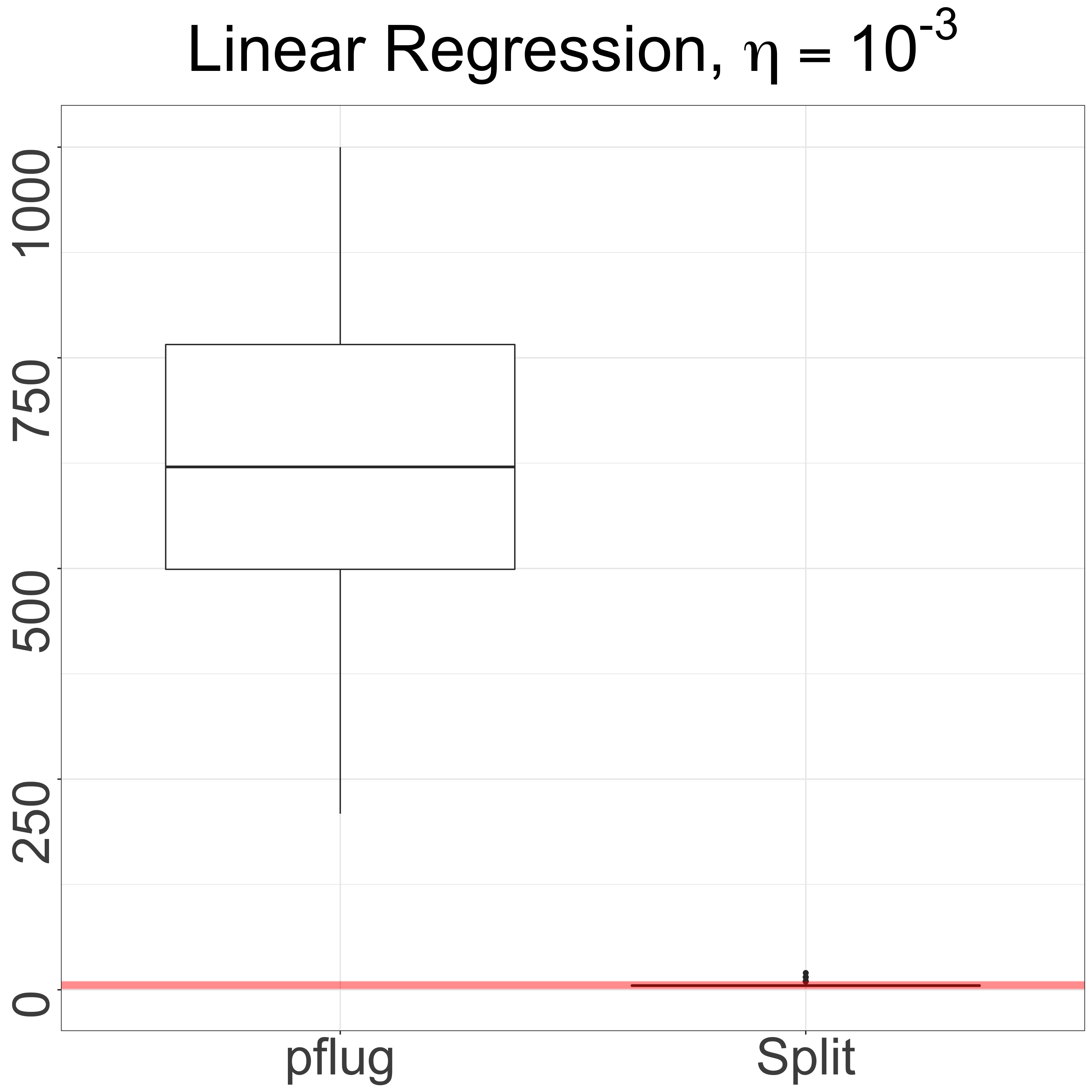
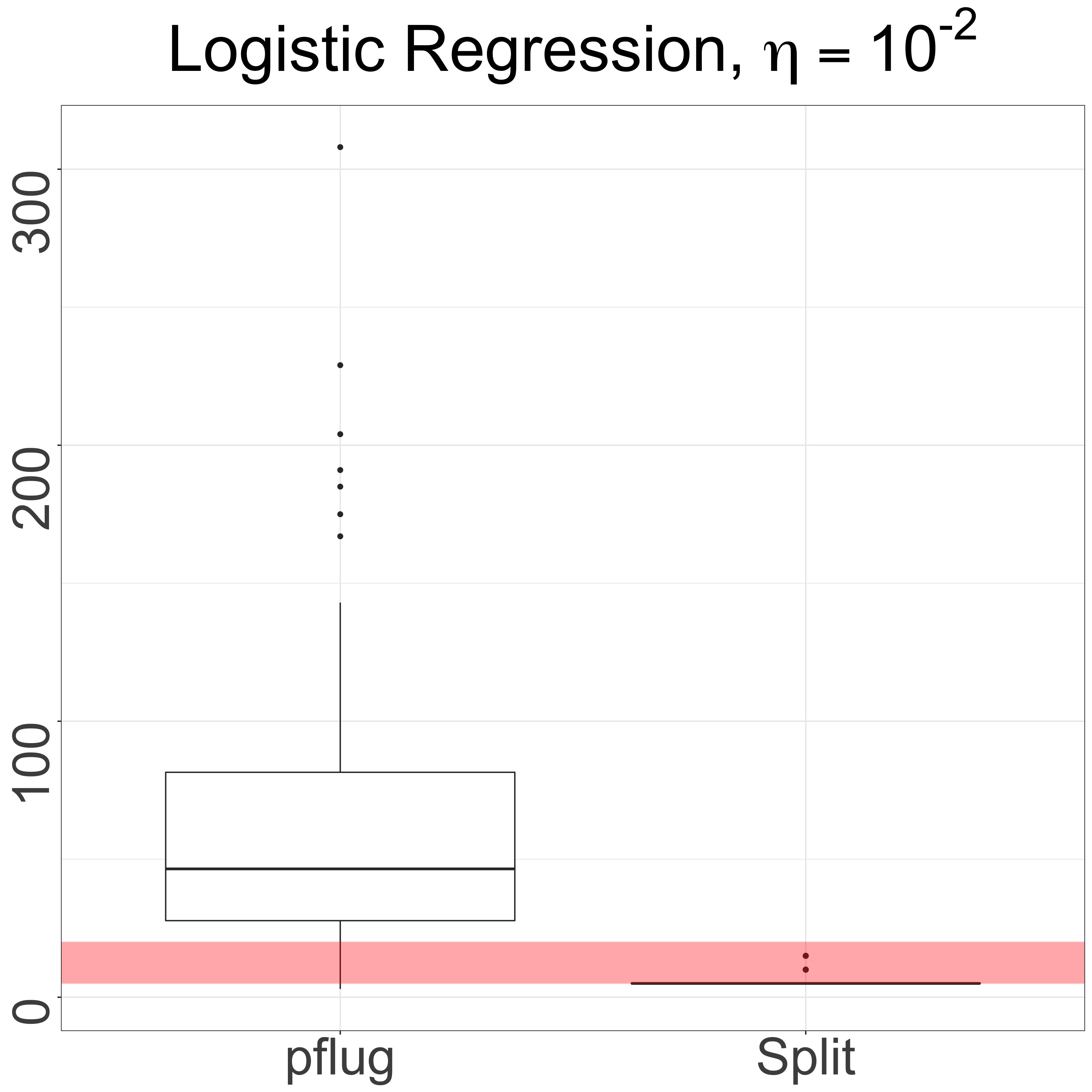
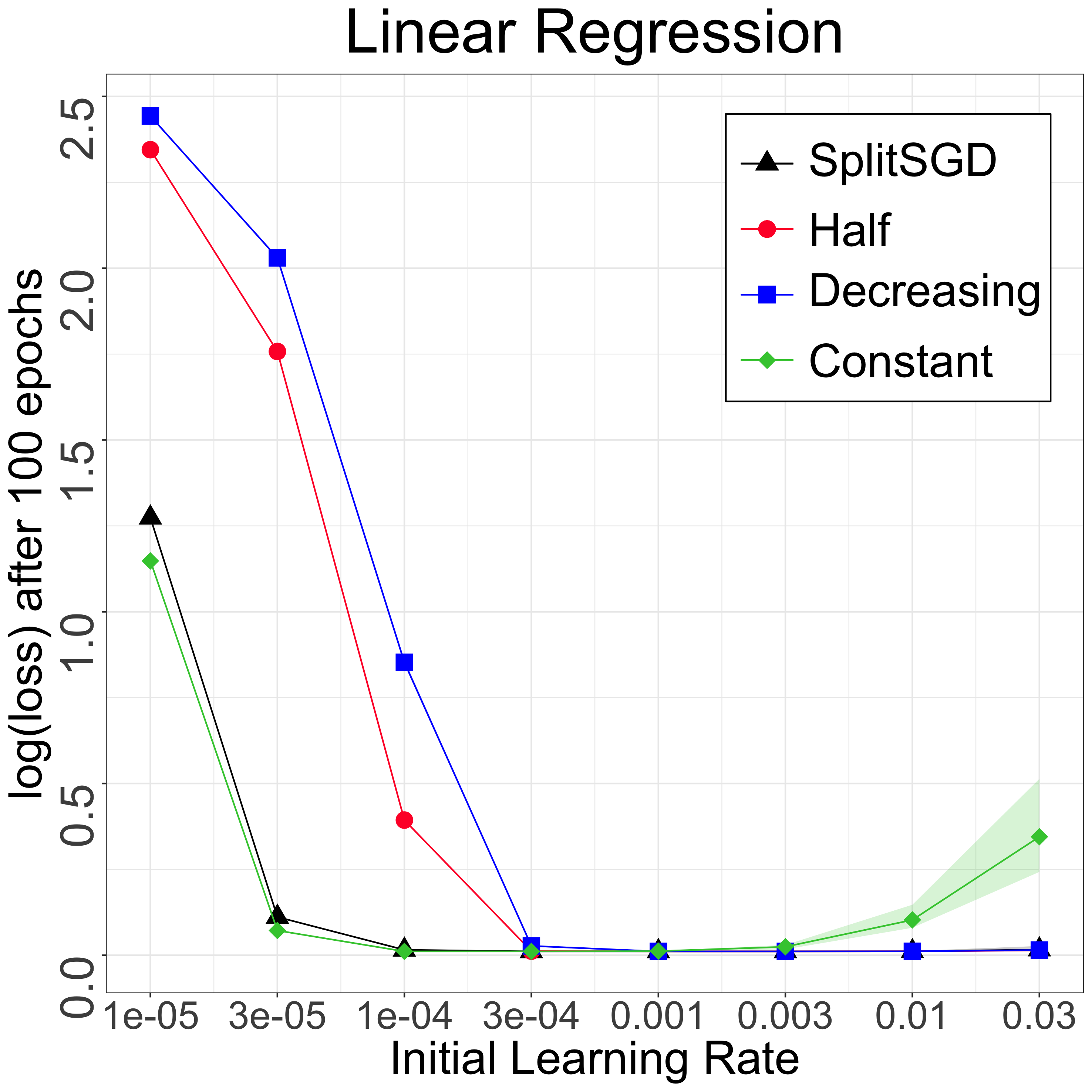
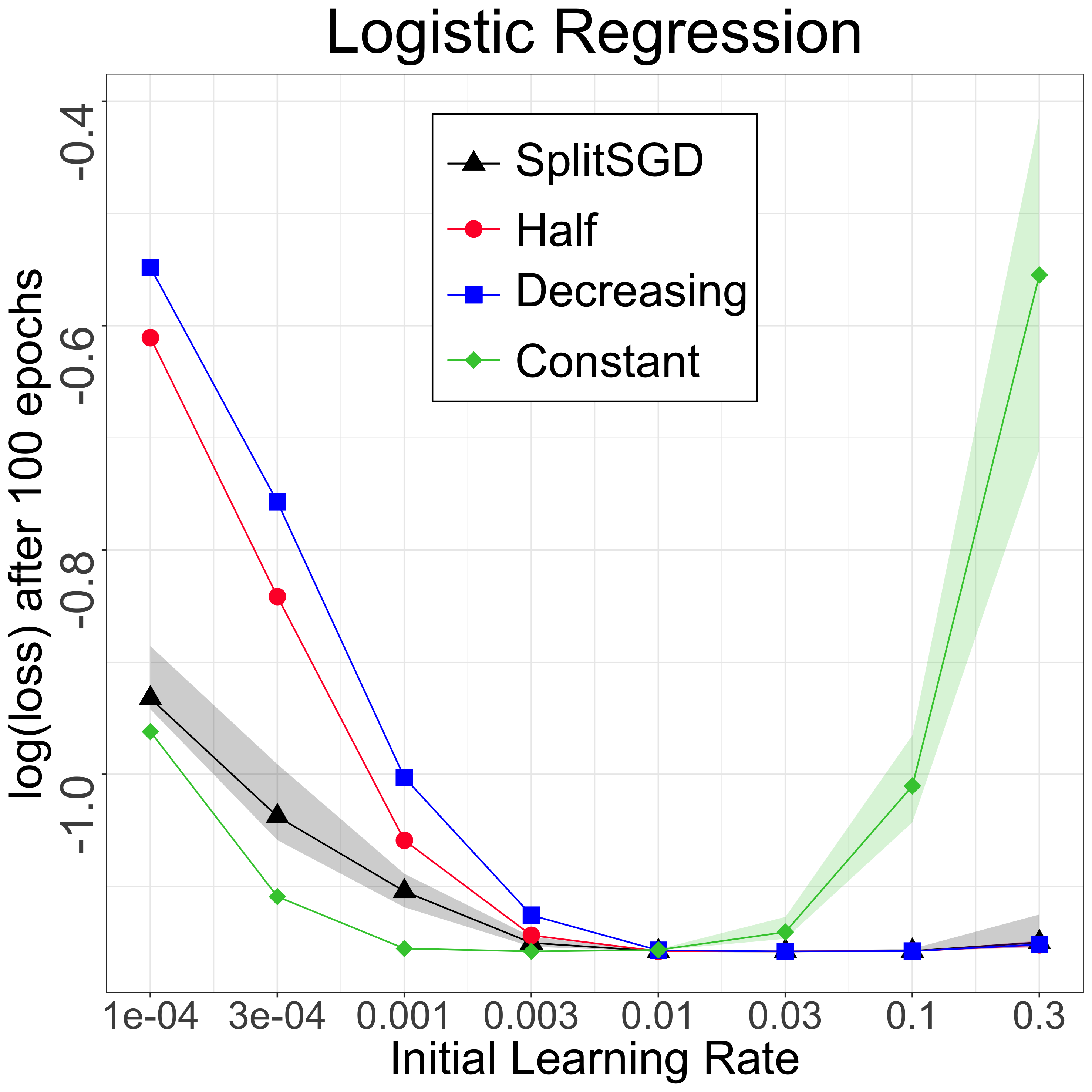
Figure 4: (top) comparison between Splitting and pflug Diagnostics on linear and logistic regression. The red bands are the epochs where stationarity should be detected. (bottom) comparison of the log(loss) achieved after $100$ epochs between SplitSGD, SGD^1/2 (Half) and SGD with constant or decreasing learning rate on linear and logistic regression. More details are in Section 4.1.

4 Experiments

4.1 Convex Objective

The setting is described in details in Appendix E.1. We use a feature matrix $X\in\mathbb{R}^{n\times d}$ with standard normal entries and $n=1000$, $d=20$ and $\theta^{*}_{j}=5\cdot e^{-j/2}$ for $j=1,...,20$. The key parameters are $t_{1}=4,w=20,l=50$ and $q=0.4$. A sensitivity analysis is in Section 4.3.

Comparison between splitting and pflug diagnostic. In the left panels of Figure 4 we compare the Splitting Diagnostic with the pflug Diagnostic introduced in Chee and Toulis, (2018). The boxplots are obtained running both diagnostic procedures from a starting point $\theta_{0}=\theta_{s}+\epsilon^{\prime}$, where $\epsilon^{\prime}\sim N(0,0.01I_{d})$ is multivariate Gaussian and $\theta_{s}$ has the same entries of $\theta^{*}$ but in reversed order, so $\theta_{s,j}=5\cdot e^{-(d-j)/2}$ for $j=1,...,20$. Each experiment is repeated $100$ times. For the Splitting Diagnostic, we run SplitSGD and declare that stationarity has been detected at the first time that a diagnostic gives result $T_{D}=S$, and output the number of epochs up to that time. For the pflug diagnostic, we stop when the running sum of dot products used in the procedure becomes negative at the end of an epoch. The maximum number of epochs is $1000$, and the red horizontal bands represent the approximate values for when we can assume that stationarity has been reached, based on when the loss function of SGD with constant learning rate stops decreasing. We can see that the result of the Splitting Diagnostic is close to the truth, while the pflug Diagnostic incurs the risk of waiting for too long, when the initial dot products of consecutive noisy gradients are positive and large compared to the negative increments after stationarity is reached. The Splitting Diagnostic does not have this problem, as a checkpoint is set every fixed number of iterations. The previous computations are then discarded, and only the new learning rate and starting point are stored. In Appendix E.2 we show more configurations of learning rates and starting points.

Comparison between SplitSGD and other optimization procedures. Here we set the decay rate to the standard value $\gamma=0.5$, and compare SplitSGD with SGD with constant learning rate $\eta$, SGD with decreasing learning rate $\eta_{t}\propto 1/\sqrt{t}$ (where the initial learning rate is set to $20\eta$), and SGD^1/2 (Bottou et al.,, 2018), where the learning rate is halved deterministically and the length of the next thread is double that of the previous one. For SGD^1/2 we set the length of the initial thread to be $t_{1}$, the same as for SplitSGD. In the right panels of Figure 4 we report the log of the loss that we achieve after $100$ epochs for different choices of the initial learning rate. It is clear that keeping the learning rate constant is optimal when its initial value is small, but becomes problematic for large initial values. On the contrary, deterministic decay can work well for larger initial learning rates but performs poorly when the initial value is small. Here, SplitSGD shows its robustness with respect to the initial choice of the learning rate, performing well on a wide range of initial learning rates.

4.2 Deep Neural Networks

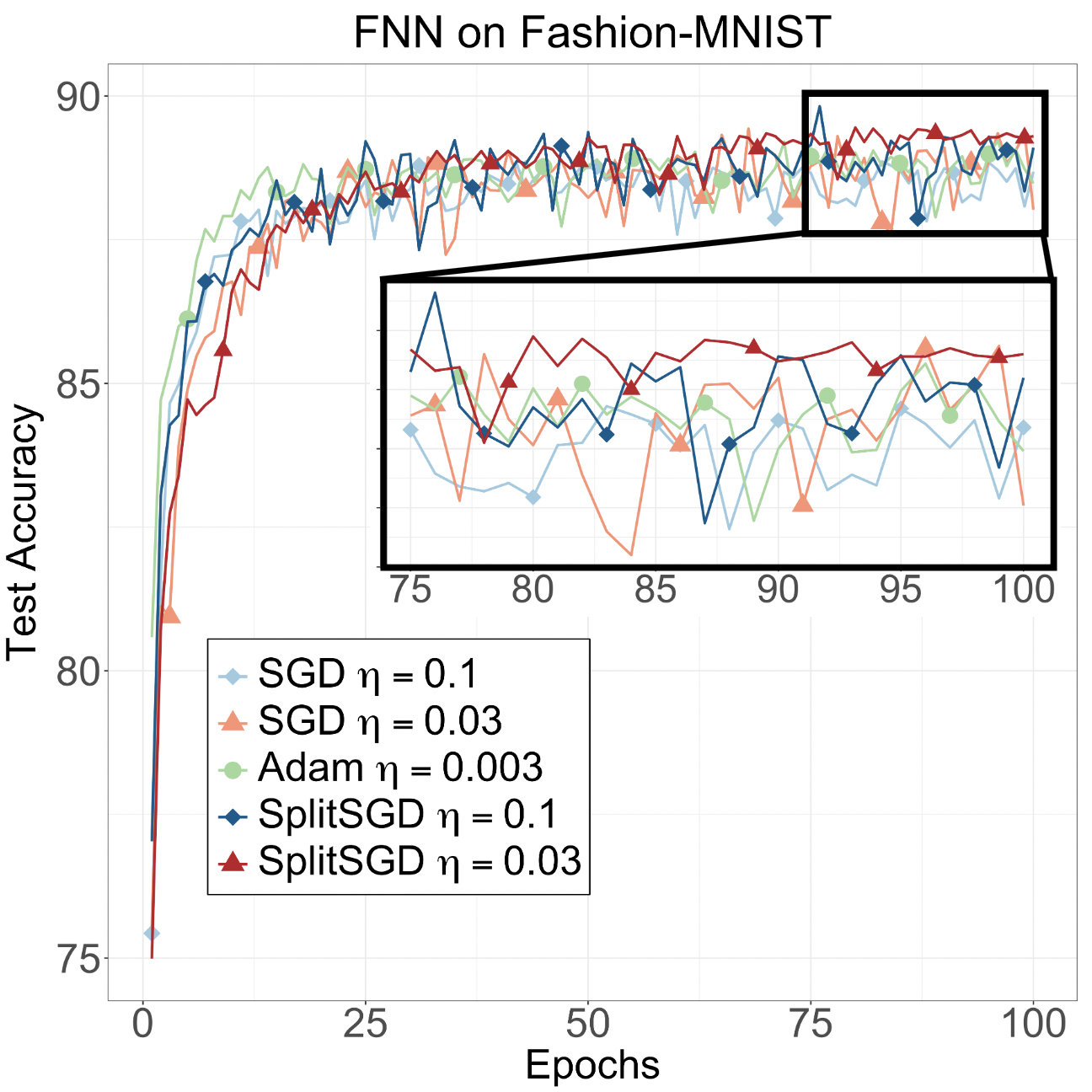
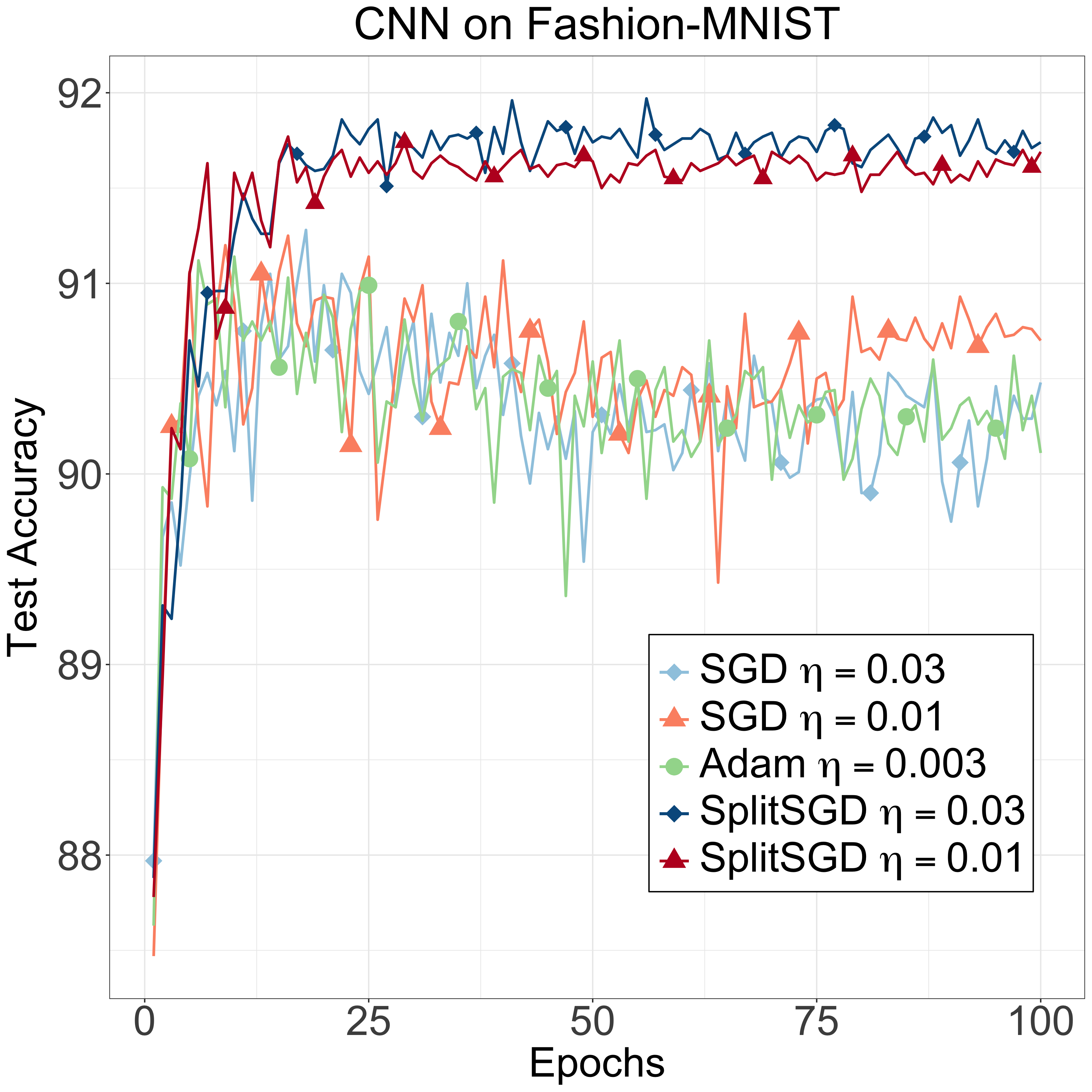
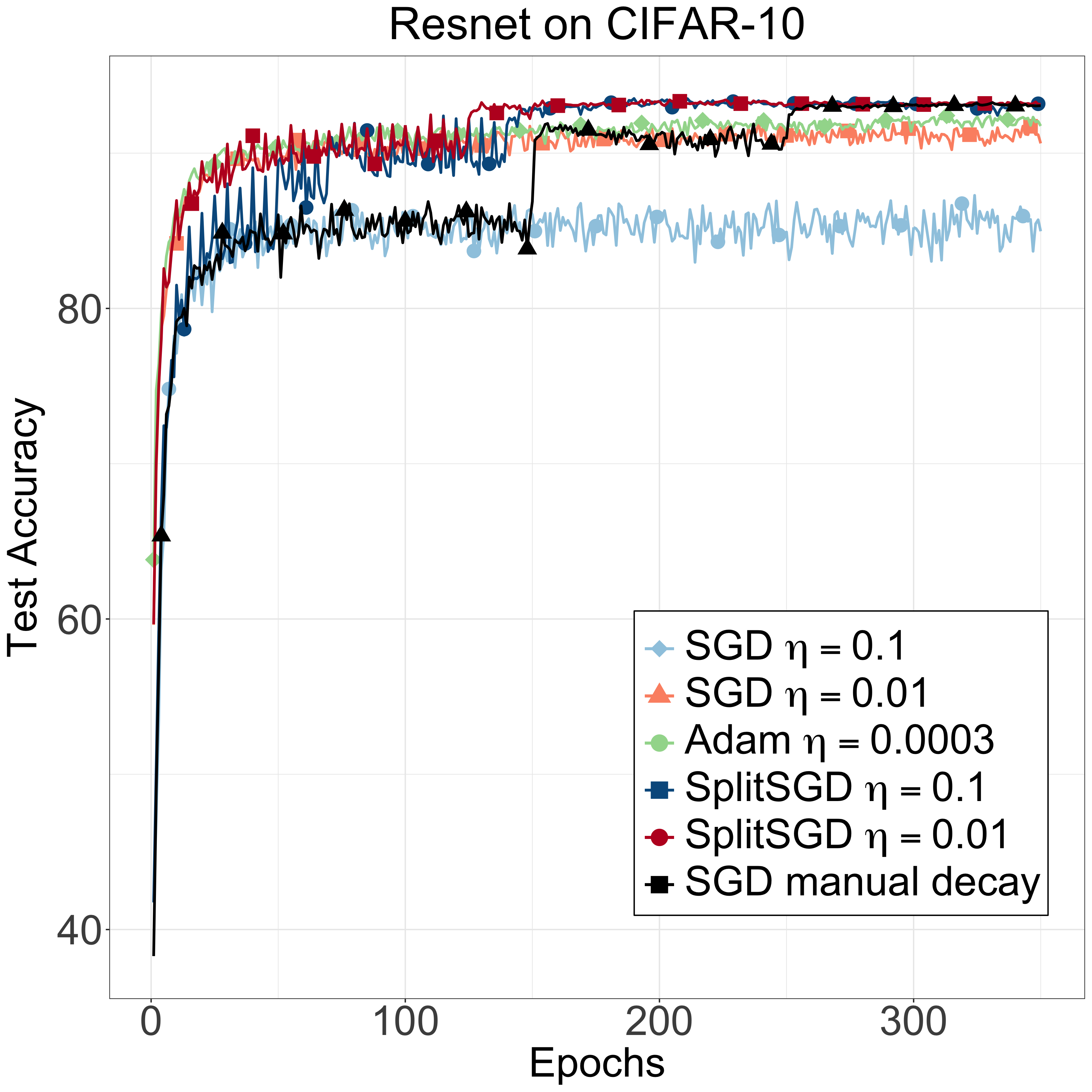
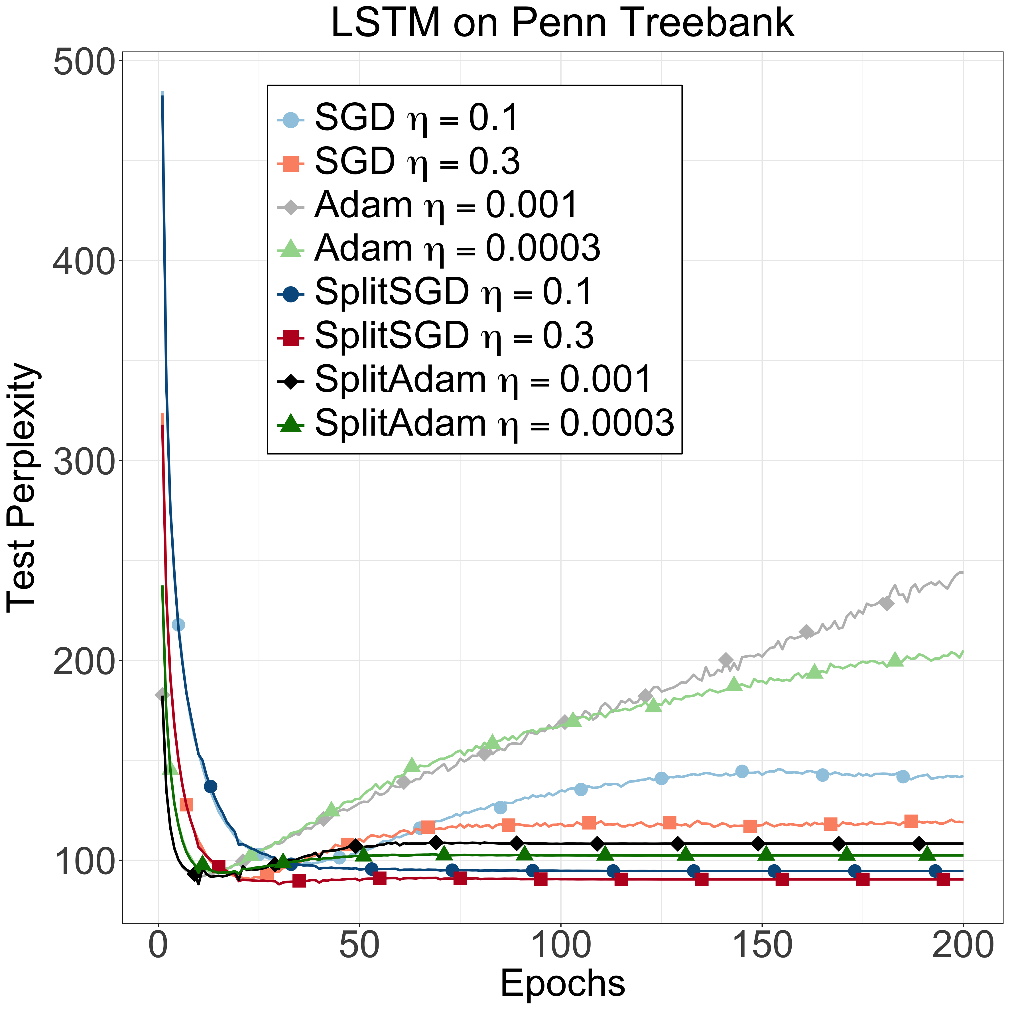
Figure 5: Performance of SGD, Adam and SplitSGD in training different neural networks. SplitSGD proved to be beneficial in (i) achieving higher test accuracy when possible, and (ii) reducing the effect of overfitting. Details of each plot are in Section 4.2.

To train deep neural networks, instead of using the simple SGD with a constant learning rate inside the SplitSGD procedure, we adopt SGD with momentum (Qian,, 1999), where the momentum parameter is set to $0.9$. SGD with momentum is a popular choice in training deep neural networks (Sutskever et al.,, 2013), and when the learning rate is constant, it still exhibits both transient and stationary phase. We introduce three more differences with respect to the convex setting: (i) the gradient coherences are defined for each layer of the network separately, then counted together to globally decay the learning rate for the whole network, (ii) the length of the single thread is not increased if stationarity is detected, and (iii) we consider the default parameters $q=0.25$ and $w=4$ for each layer. The length of the Diagnostic is again set to be one epoch. We compare SplitSGD with SGD with momentum and Adam (Kingma and Ba,, 2014). Notice that, although $\eta=$310-4$$ is the popular default value for Adam, this method is still sensitive to the choice of the learning rate, so the best performance can be achieved by other learning rates. It has also been proved that SGD generalises better than Adam (Keskar and Socher,, 2017; Luo et al.,, 2019). We will show that in many situations SplitSGD, using the same default set of parameters, can outperform both.

Feedforward neural networks (FNNs). We train a FNN with three hidden layers of size $256,128$ and $64$ on the Fashion-MNIST dataset (Xiao et al.,, 2017). The network is fully connected, with ReLu activation functions. The initial learning rates are $\eta\in\{$110-2$,$310-2$,$110-1$\}$ for SGD and SplitSGD and $\eta\in\{$310-4$,$110-3$,$310-3$\}$ for Adam. We report, here and in the next experiments, the ones that show the best results. In the first panel of Figure 5 we see that most methods achieve very good accuracy, but SplitSGD reaches the overall best test accuracy when $\eta=$110-1$$ and great accuracy with small oscillations when $\eta=$310-2$$. The peaks in the SplitSGD performance are usually due to the averaging, while the smaller oscillations are due to the learning rate decay.

Convolutional neural networks (CNNs). We consider a CNN with two convolutional layers and a final linear layer, again on the Fashion-MNIST dataset. Here we set $\eta\in\{$110-2$,$310-2$,$110-1$\}$ for SGD and SplitSGD and $\eta\in\{$310-4$,$110-3$,$310-3$,$110-2$\}$ for Adam. In the second panel of Figure 5 we observe the interesting fact that both SGD and Adam show obvious signs of overfitting, after reaching their peak around epoch $20$. SplitSGD, on the contrary, does not incur in this problem, probably for a combined effect of the averaging and learning rate decay.

Residual neural networks (ResNets). For ResNets, we consider a 18-layer ResNet and evaluate it on the CIFAR-10 dataset (Krizhevsky et al.,, 2009). We use the initial learning rates $\eta\in\{$110-3$,$110-2$,$110-1$\}$ for SGD and SplitSGD and $\eta\in\{$310-5$,$310-4$,$310-3$\}$ for Adam, and also consider the SGD procedure with manual decay that consists in setting $\eta=$110-1$$ and then decreasing it by a factor $10$ at epoch $150$ and $250$. In the third panel of Figure 5 we clearly see a classic behavior for SplitSGD. The averaging after the diagnostics makes the test accuracy peak, but the improvement is only momentary is the learning rate is not decreased. When the decay happens, the peak is maintained and the fluctuations get smaller. We can see that SplitSGD, with both initial learning rate $\eta=$110-2$$ and $\eta=$110-1$$ is better than both SGD and Adam and achieves the same final test accuracy of the manually tuned method in less epochs. In Appendix E.3 we see a very similar result obtained with the neural network VGG19.

Recurrent neural networks (RNNs). For RNNs, we evaluate a two-layer LSTM (Hochreiter and Schmidhuber,, 1997) model on the Penn Treebank (Marcus et al.,, 1993) language modeling task. We use $\eta\in\{0.1,0.3,1.0\}$ for both SGD and SplitSGD, $\eta\in\{$110-4$,$310-4$,$110-3$\}$ for Adam and introduce SplitAdam, a method similar to SplitSGD, but with Adam in place of SGD with momentum. As shown in the fourth panel of Figure 5, we can see that SplitSGD outperforms SGD and SplitAdam outperforms Adam with regard to both the best performance and the last performance. Similar to what already observed with the CNN, we need to note that our proposed splitting strategy has the advantage of reducing the effect of overfitting. We postpone the theoretical understanding for this phenomena as our future work.

For the four types of deep neural networks considered, FNNs, CNNs, ResNets, and RNNs, SplitSGD shows better results compared to SGD and Adam, and exhibits strong robustness to the choice of initial learning rates, which further verifies the effectiveness of SplitSGD in deep neural networks.

4.3 Sensitivity Analysis for SplitSGD

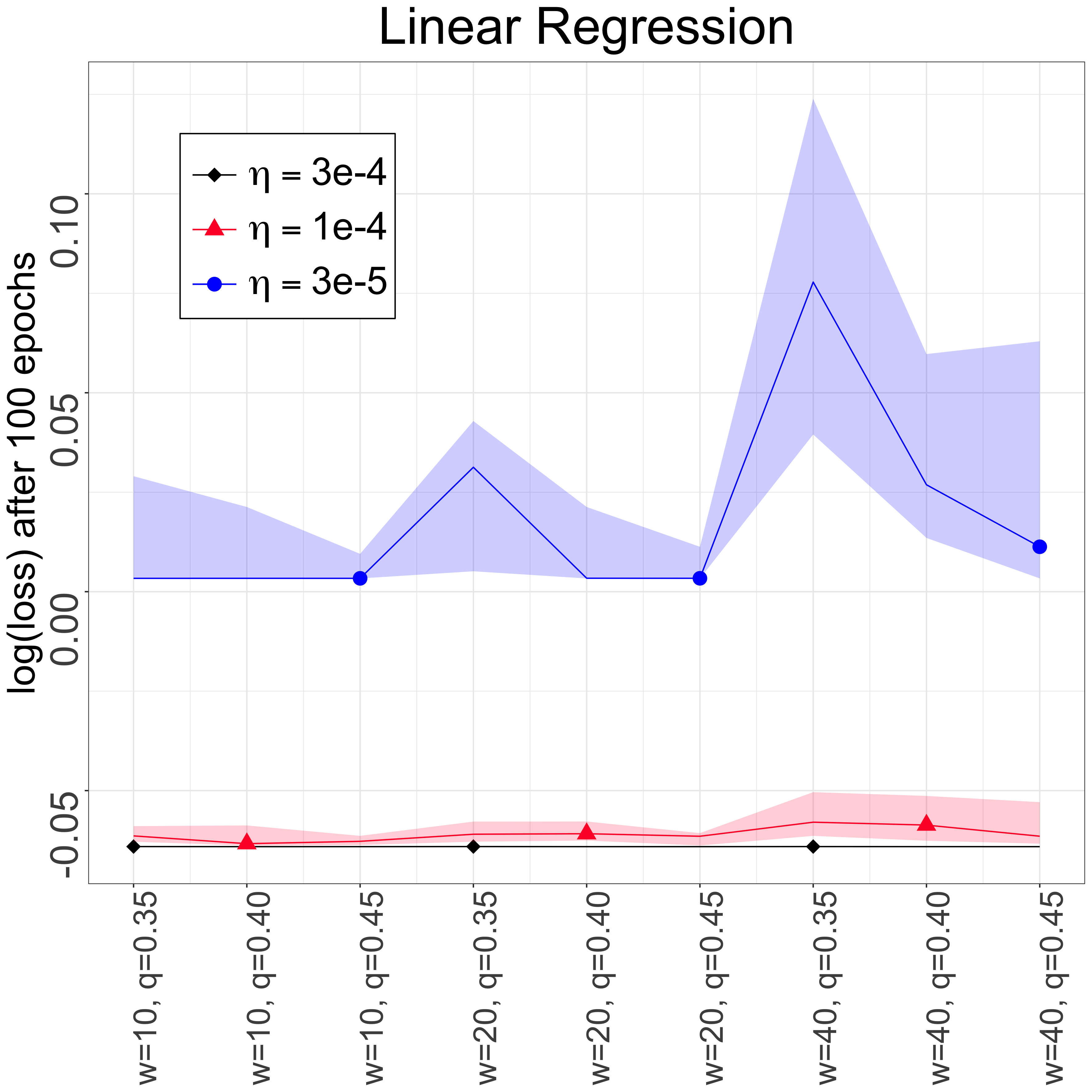
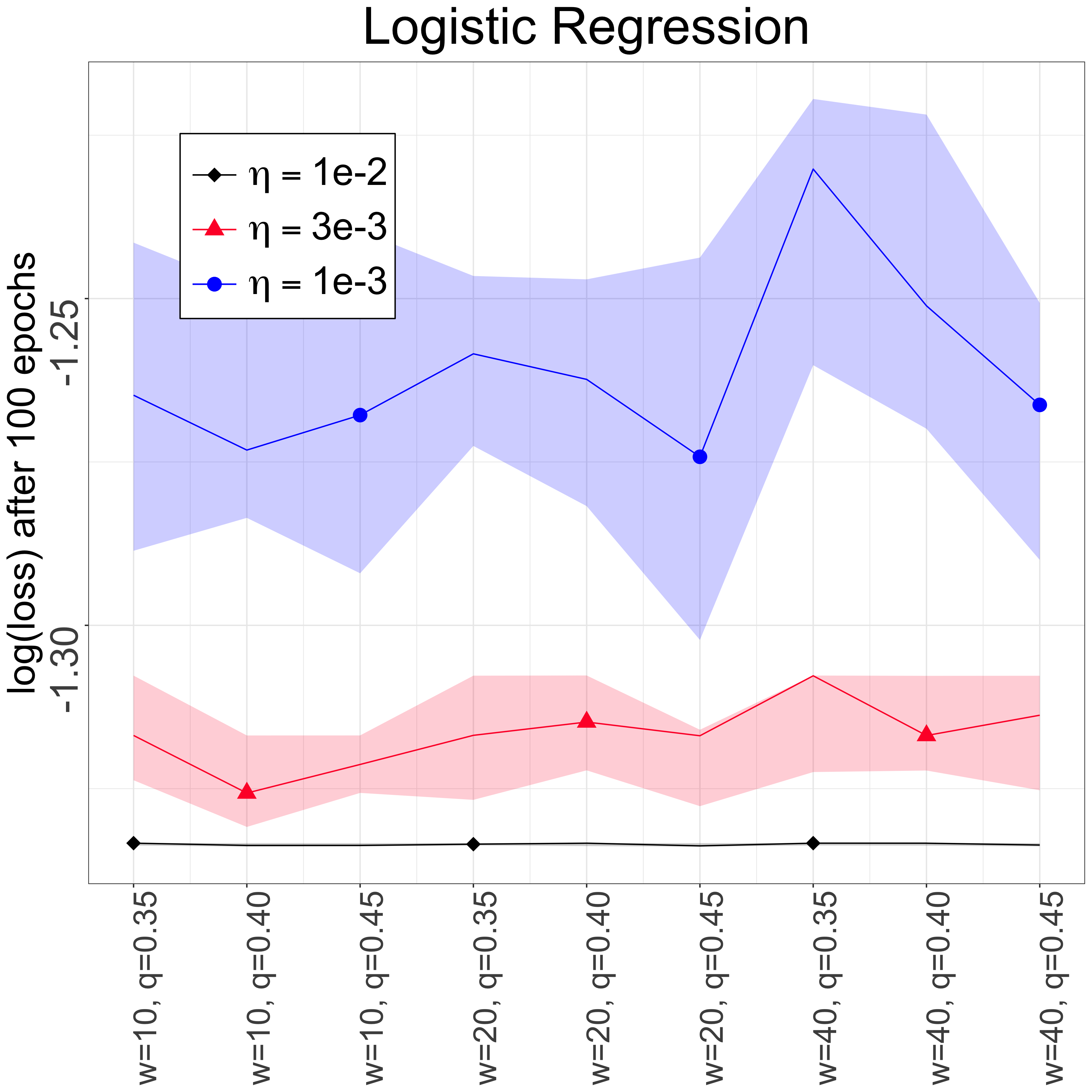
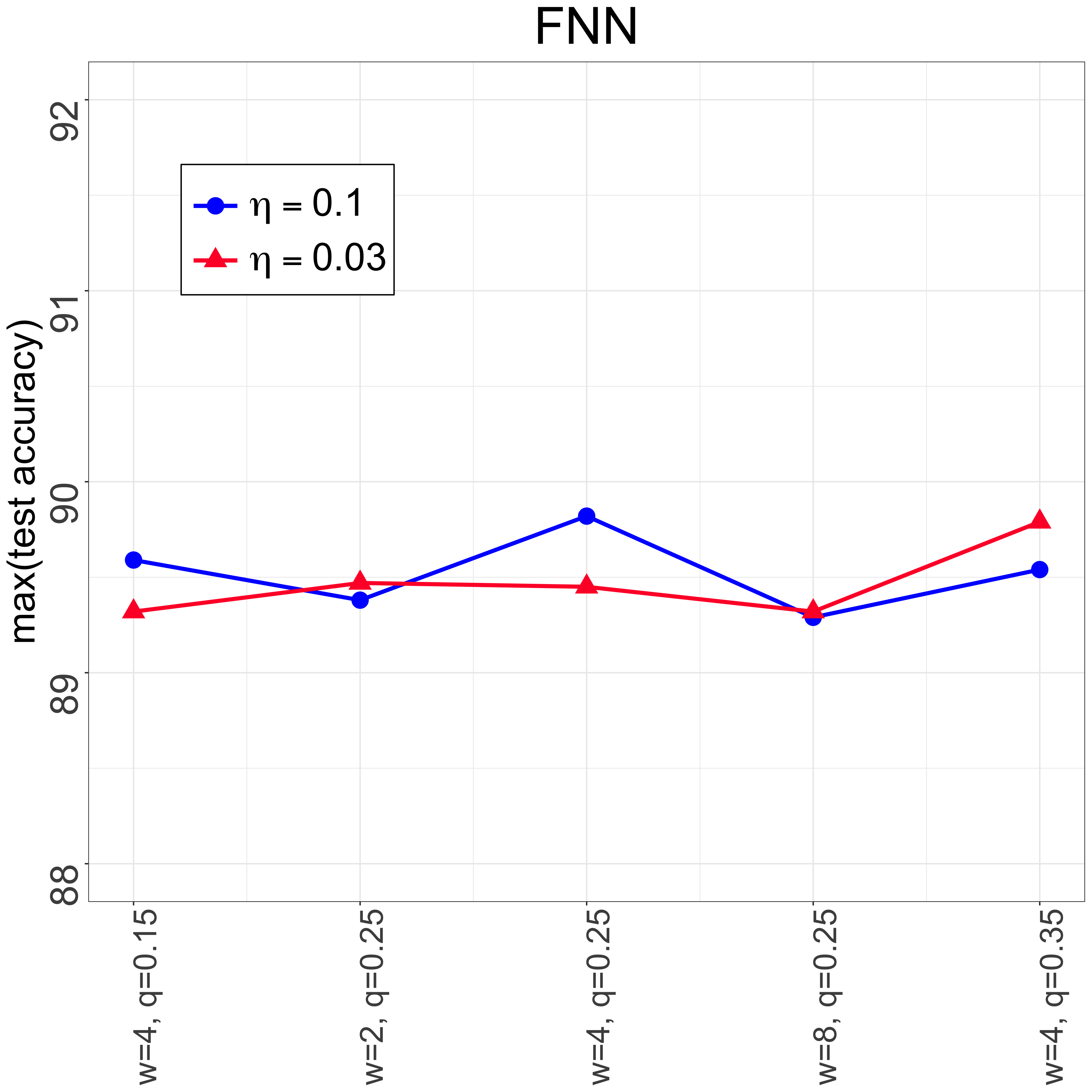
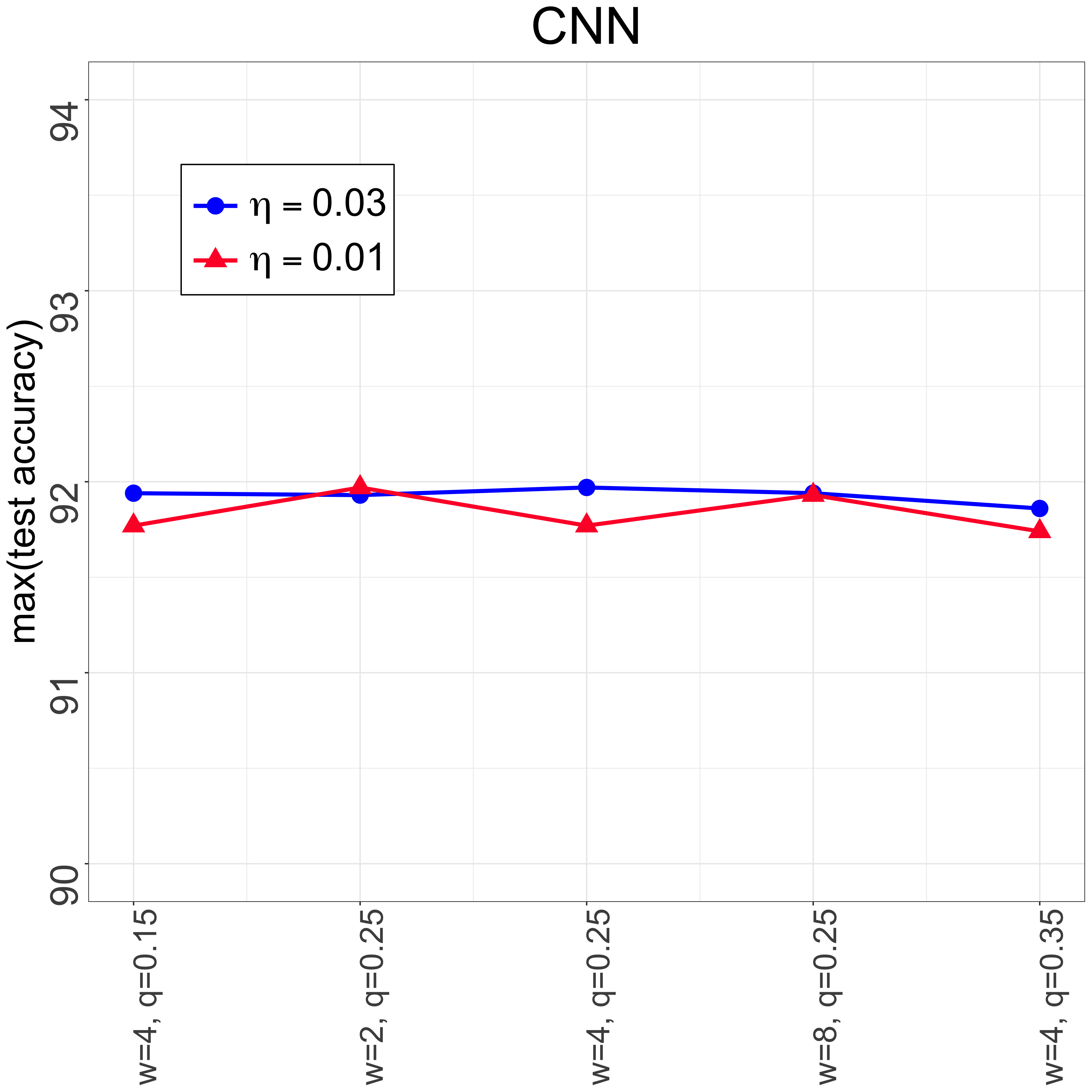
Figure 6: Sensitivity analysis for SplitSGD with respect to the parameters $w$ and $q$. In the convex setting (top) we consider the log loss achieved after $100$ epochs, while for deep neural networks (bottom) we report the maximum of the test accuracy. Details in Section 4.3.

In this section, we analyse the impact of the hyper-parameters in the SplitSGD procedure. We focus on $q$ and $w$, while $l$ changes so that the computational budget of each diagnostic is fixed at one epoch. In the left panels of Figure 6 we analyse the sensitivity of SplitSGD to these two parameters in the convex setting, and consider $w\in\{10,20,40\}$ and $q\in\{0.35,0.40,0.45\}$. We report the log(loss) after training for $100$ epochs. The results are as expected; when the initial learning rate is larger, the impact of these parameters is very modest. When the initial learning rate is small, having a quicker decay (i.e. setting $q$ smaller) worsen the performance.

In the right panels of Figure 6 we see the same analysis applied to the FNNs and the CNNs trained on Fashion-MNIST. Here we report the maximum test accuracy achieved when training for $100$ epochs, and on the x-axis we have various configurations for $w\in\{0.15,0,25,0.35\}$ and $q\in\{2,4,8\}$. The results are very encouraging, showing that SplitSGD is robust with respect to the choice of these parameters also in non-convex settings.

5 Conclusion and Future Work

We have developed an efficient optimization method called SplitSGD, by splitting the SGD thread for stationarity detection. Extensive simulation studies show that this method is robust to the choice of the initial learning rate in a variety of optimization tasks, compared to classic non-adaptive methods. Moreover, SplitSGD on certain deep neural network architectures outperforms classic SGD and Adam in terms of the test accuracy, and can sometime limit greatly the impact of overfitting. As the critical element underlying SplitSGD, the Splitting Diagnostic is a simple yet effective strategy that can possibly be incorporated into many optimization methods beyond SGD, as we already showed training SplitAdam on LSTM. One possible limitation of this method is the introduction of a new relevant parameter $q$, that regulates the rate at which the learning rate is adaptively decreased. Our simulations suggest the use of two different values depending on the context. A slower decrease, $q=0.4$, in convex optimization, and a more aggressive one, $q=0.25$, for deep learning. In the future, we look forward to seeing research investigations toward boosting the convergence of SplitSGD by allowing for different learning rate selection strategies across different layers of the neural networks.

Appendix A Lemmas

Lemma A.1.

If Assumptions 3.1, 3.2, 3.3 and 3.4 with $m=2$ hold, and $\eta\leq\frac{\mu}{L^{2}}$, then for any $t\geq 0$

$${}\operatorname{\mathbb{E}}\left[\|\theta_{t}-\theta^{*}\|^{2}\right] \leq\left(1-2\eta(\mu-L^{2}\eta)\right)^{t}\cdot\operatorname{\mathbb{E}}\left[\|\theta_{0}-\theta^{*}\|^{2}\right]$$

$$\quad+\frac{G^{2}\eta}{\mu-L^{2}\eta}.$$

Proof.

This proof can be easily adapted from Moulines and Bach, (2011). From the recursive definition of $\theta_{t}$ one has

$$\operatorname{\mathbb{E}}\left[||\theta_{t}-\theta^{*}||^{2}\right]\leq\left(1-2\eta(\mu-L^{2}\eta)\right)\cdot\operatorname{\mathbb{E}}\left[||\theta_{t-1}-\theta^{*}||^{2}\right]+2G^{2}\eta^{2}.$$

This inequality can be recursively applied to obtain the desired result

$$\operatorname{\mathbb{E}}\left[||\theta_{t}-\theta^{*}||^{2}\right] \leq\left(1-2\eta(\mu-L^{2}\eta)\right)^{t}\cdot\operatorname{\mathbb{E}}\left[||\theta_{0}-\theta^{*}||^{2}\right]+2G^{2}\eta^{2}\sum_{j=0}^{t-1}\left(1-2\eta(\mu-L^{2}\eta)\right)^{j}$$

$$\leq\left(1-2\eta(\mu-L^{2}\eta)\right)^{t}\cdot\operatorname{\mathbb{E}}\left[||\theta_{0}-\theta^{*}||^{2}\right]+\frac{G^{2}\eta}{\mu-L^{2}\eta}$$

∎

This lemma represents the dynamic of SGD with constant learning rate, where the dependence from the starting point vanishes exponentially fast, but there is a term dependent on $\eta$ that is not vanishing even for large $t$.

Lemma A.2.

If Assumption 3.4 with $m=4$ holds, then for any $t,i\in\mathcal{N}$ one has

$$\operatorname{\mathbb{E}}\left[||\theta_{t+i}-\theta_{t}||^{4}\ |\ \mathcal{F}_{t}\right]\leq\eta^{4}i^{4}G^{4}$$

Proof.

For any $j=1,...,l$, let $x_{j}$ be a vector of length $n$. Applying Cauchy-Schwarz inequality twice, we get

$${}||\sum_{j=1}^{l}x_{j}||^{4} =||\sum_{j=1}^{l}x_{j}||^{2}\cdot||\sum_{j=1}^{l}x_{j}||^{2}\leq\left(l\cdot\sum_{j=1}^{l}||x_{j}||^{2}\right)^{2}$$

$$=l^{2}\left(\sum_{j=1}^{l}||x_{j}||^{2}\right)^{2}\leq l^{3}\cdot\sum_{j=1}^{l}||x_{j}||^{4}$$ (A.1)

Since

$$\theta_{t+i}=\theta_{t}-\eta\sum_{j=0}^{i-1}g(\theta_{t+j},Z_{t+j+1}),$$

then we can use the fact that $\mathcal{F}_{k}\subseteq\mathcal{F}_{k+1}$ for any $k$, together with Assumption 3.4 and (A), to get that

$$\operatorname{\mathbb{E}}\left[||\theta_{t+i}-\theta_{t}||^{4}\ |\ \mathcal{F}_{t}\right] =\eta^{4}\cdot\operatorname{\mathbb{E}}\left[||\sum_{j=0}^{i-1}g(\theta_{t+j},Z_{t+j+1})||^{4}\ |\ \mathcal{F}_{t}\right]$$

$$\leq\eta^{4}i^{3}\sum_{j=0}^{i-1}\operatorname{\mathbb{E}}\left[||g(\theta_{t+j},Z_{t+j+1})||^{4}\ |\ \mathcal{F}_{t}\right]$$

$$=\eta^{4}i^{3}\sum_{j=0}^{i-1}\operatorname{\mathbb{E}}\big{[}\underbrace{\operatorname{\mathbb{E}}\left[||g(\theta_{t+j},Z_{t+j+1})||^{4}\ |\ \mathcal{F}_{t+j}\right]}_{\qquad\leq G^{4}}\ \big{|}\ \mathcal{F}_{t}\big{]}$$

$$\leq\eta^{4}i^{4}G^{4}$$

Note that this is a bound that considers the worst case in which all the noisy gradient updates point in the same direction and are of norm $G$. ∎

Remark A.3.

We can obviously use the same bound for the unconditional squared norm, since

$$\operatorname{\mathbb{E}}\left[||\theta_{t+i}-\theta_{t}||^{4}\right]=\operatorname{\mathbb{E}}\left[\operatorname{\mathbb{E}}\left[||\theta_{t+i}-\theta_{t}||^{4}\ |\ \mathcal{F}_{t}\right]\right]\leq\eta^{4}i^{4}G^{4}.$$

Lemma A.4.

If Assumption 3.2 and 3.4 with $m=2$ hold, then for any $i=1,...,l$ and $k=1,2$ we have that

$$\operatorname{\mathbb{E}}\left[||\nabla F(\theta_{t+i}^{(k)})-\nabla F(\theta_{0})||^{2}\ |\ \mathcal{F}_{t}\right]\leq(L||\theta_{t}-\theta_{0}||+L\eta Gi)^{2}$$

Proof.

By adding and subtracting $\nabla F(\theta_{t})$, and by Lemma A.2, we get.

$$\operatorname{\mathbb{E}}\left[||\nabla F(\theta_{t+i}^{(k)})-\nabla F(\theta_{0})||^{2}\ |\ \mathcal{F}_{t}\right]\leq\operatorname{\mathbb{E}}\left[||\nabla F(\theta_{t+i}^{(k)})-\nabla F(\theta_{t})+\nabla F(\theta_{t})-\nabla F(\theta_{0})||^{2}\ |\ \mathcal{F}_{t}\right]$$

$$\qquad\leq||\nabla F(\theta_{t})-\nabla F(\theta_{0})||^{2}+\operatorname{\mathbb{E}}\left[||\nabla F(\theta_{t+i}^{(k)})-\nabla F(\theta_{t})||^{2}\ |\ \mathcal{F}_{t}\right]$$

$$\qquad\quad+2||\nabla F(\theta_{t})-\nabla F(\theta_{0})||\cdot\operatorname{\mathbb{E}}\left[||\nabla F(\theta_{t+i}^{(k)})-\nabla F(\theta_{t})||\ |\ \mathcal{F}_{t}\right]$$

$$\qquad\leq L^{2}||\theta_{t}-\theta_{0}||^{2}+L^{2}\operatorname{\mathbb{E}}\left[||\theta_{t+i}^{(k)}-\theta_{t}||^{2}\ |\ \mathcal{F}_{t}\right]+2L^{2}||\theta_{t}-\theta_{0}||\cdot\operatorname{\mathbb{E}}\left[||\theta_{t+i}^{(k)}-\theta_{t}||\ |\ \mathcal{F}_{t}\right]$$

$$\qquad\leq L^{2}||\theta_{t}-\theta_{0}||^{2}+L^{2}\eta^{2}G^{2}i^{2}+2L^{2}||\theta_{t}-\theta_{0}||\eta Gi$$

$$\qquad=(L||\theta_{t}-\theta_{0}||+L\eta Gi)^{2}$$

∎

Remark A.5.

When we consider the unconditional distance of the gradients, we can simply use smoothness and Remark A.3 to get

$$\operatorname{\mathbb{E}}\left[||\nabla F(\theta_{t+i}^{(k)})-\nabla F(\theta_{0})||^{2}\right]\leq L^{2}\operatorname{\mathbb{E}}\left[||\theta_{t+i}^{(k)}-\theta_{0}||^{2}\right]\leq L^{2}\eta^{2}G^{2}(t+i)^{2}$$

which is the same result that we obtain from Lemma A.4 if at the end we bound $||\theta_{t}-\theta_{0}||$ with its expectation, and use the fact that $\operatorname{\mathbb{E}}\left[||\theta_{t}-\theta_{0}||\right]\leq\eta Gt$.

Lemma A.6.

If Assumption 3.2 and 3.4 with $m=2$ hold, then for any $i=1,...,l$ and $k=1,2$ we have that

• $\operatorname{\mathbb{E}}\left[||\nabla F(\theta_{t+i}^{(k)})||^{2}\ |\ \mathcal{F}_{t}\right]\leq(||\nabla F(\theta_{0})||+L||\theta_{t}-\theta_{0}||+L\eta Gi)^{2}$

• $\operatorname{\mathbb{E}}\left[||\nabla F(\theta_{t+i}^{(k)})||^{2}\ |\ \mathcal{F}_{t}\right]\leq(L||\theta_{t}-\theta^{*}||+L\eta Gi)^{2}$

Proof.

We add and subtract $\nabla F(\theta_{t})$ to the gradient on the left hand side, and apply Lemma A.2.

$$\operatorname{\mathbb{E}}\left[||\nabla F(\theta_{t+i}^{(k)})||^{2}\ |\ \mathcal{F}_{t}\right]=\operatorname{\mathbb{E}}\left[||\nabla F(\theta_{t+i}^{(k)})-\nabla F(\theta_{t})+\nabla F(\theta_{t})||^{2}\ |\ \mathcal{F}_{t}\right]$$

$$\qquad\leq||\nabla F(\theta_{t})||^{2}+\operatorname{\mathbb{E}}\left[||\nabla F(\theta_{t+i}^{(k)})-\nabla F(\theta_{t})||^{2}\ |\ \mathcal{F}_{t}\right]$$

$$\qquad\quad+2||\nabla F(\theta_{t})||\cdot\operatorname{\mathbb{E}}\left[||\nabla F(\theta_{t+i}^{(k)})-\nabla F(\theta_{t})||\ |\ \mathcal{F}_{t}\right]$$

$$\qquad\leq||\nabla F(\theta_{t})||^{2}+L^{2}\operatorname{\mathbb{E}}\left[||\theta_{t+i}^{(k)}-\theta_{t}||^{2}\ |\ \mathcal{F}_{t}\right]+2L||\nabla F(\theta_{t})||\cdot\operatorname{\mathbb{E}}\left[||\theta_{t+i}^{(k)}-\theta_{t}||\ |\ \mathcal{F}_{t}\right]$$

$$\qquad\leq||\nabla F(\theta_{t})||^{2}+L^{2}\eta^{2}G^{2}i^{2}+2||\nabla F(\theta_{t})||\cdot L\eta Gi$$ (A.2)

To get part $i)$ we repeat the same trick, this time adding and subtracting $\nabla F(\theta_{0})$ to the terms that contain $\nabla F(\theta_{t})$.

$$(\ref{gradient_condition_Ft_temp}) \leq||\nabla F(\theta_{0})||^{2}+||\nabla F(\theta_{t})-\nabla F(\theta_{0})||^{2}+2||\nabla F(\theta_{0})||\cdot||\nabla F(\theta_{t})-\nabla F(\theta_{0})||$$

$$\qquad\qquad+L^{2}\eta^{2}G^{2}i^{2}+2||\nabla F(\theta_{0})||\cdot L\eta Gi+2||\nabla F(\theta_{t})-\nabla F(\theta_{0})||\cdot L\eta Gi$$

$$\qquad\leq||\nabla F(\theta_{0})||^{2}+L^{2}||\theta_{t}-\theta_{0}||^{2}+2L||\nabla F(\theta_{0})||\cdot||\theta_{t}-\theta_{0}||$$

$$\qquad\qquad+L^{2}\eta^{2}G^{2}i^{2}+2||\nabla F(\theta_{0})||\cdot L\eta Gi+2||\theta_{t}-\theta_{0}||\cdot L^{2}\eta Gi$$

$$\qquad=(||\nabla F(\theta_{0})||+L||\theta_{t}-\theta_{0}||+L\eta Gi)^{2}$$

To get part $ii)$, instead, we can add $\nabla f(\theta^{*})$ and get

$$(\ref{gradient_condition_Ft_temp}) \leq L^{2}||\theta_{t}-\theta^{*}||^{2}+L^{2}\eta^{2}G^{2}i^{2}+2||\theta_{t}-\theta^{*}||\cdot L^{2}\eta Gi$$

$$=(L||\theta_{t}-\theta^{*}||+L\eta Gi)^{2}$$

∎

Remark A.7.

For the unconditional squared norm of the gradient we again obtain the same bound as if in Lemma A.6 we were considering $\operatorname{\mathbb{E}}[||\theta_{t}-\theta_{0}||]\leq\eta Gt$ instead of just the argument of the expectation.

$$\operatorname{\mathbb{E}}\left[||\nabla F(\theta_{t+i}^{(k)})||^{2}\right] =\operatorname{\mathbb{E}}\left[||\nabla F(\theta_{t+i}^{(k)})-\nabla F(\theta_{0})+\nabla F(\theta_{0})||^{2}\right]$$

$$\leq||\nabla F(\theta_{0})||^{2}+\operatorname{\mathbb{E}}\left[||\nabla F(\theta_{t+i}^{(k)})-\nabla F(\theta_{0})||^{2}\right]$$

$$\quad+2||\nabla F(\theta_{0})||\cdot\operatorname{\mathbb{E}}\left[||\nabla F(\theta_{t+i}^{(k)})-\nabla F(\theta_{0})||\right]$$

$$\leq||\nabla F(\theta_{0})||^{2}+L^{2}\eta^{2}G^{2}(t+i)^{2}+2||\nabla F(\theta_{0})||L\eta G(t+i)$$

$$=(||\nabla F(\theta_{0})||+L\eta G(t+i))^{2}$$

Appendix B Proof of Theorem 1

Proof.

To slightly simplify the notation, we consider only $Q_{1}$. For the following windows, the calculations are equal and just involve some more terms, that are negligible if $\eta$ is small enough. We assume that the Splitting Diagnostic starts after $t$ iterations have already been made. We use the idea that, for a fixed $t$, if the learning rate is sufficiently small, the SGD iterate $\theta_{t}$ and $\theta_{0}$ will not be very far apart. In particular we will use $\eta$ small enough such that $\eta\cdot(t+l)$ is small, making every term of order $O(\eta^{k}(t+l)^{k})$ negligible for $k>1$. Thanks to the conditional independence of the errors, the expectation of $Q_{1}$ can be written only in terms of the true gradients.

$${}\operatorname{\mathbb{E}}\left[Q_{1}\right] =\frac{1}{l^{2}}\sum_{i=0}^{l-1}\sum_{j=0}^{l-1}\operatorname{\mathbb{E}}\left[\langle g(\theta_{t+i}^{(1)}),g(\theta_{t+j}^{(2)})\rangle\right]$$

$$=\frac{1}{l^{2}}\sum_{i=0}^{l-1}\sum_{j=0}^{l-1}\operatorname{\mathbb{E}}\left[\langle\nabla F(\theta_{t+i}^{(1)})+\epsilon(\theta_{t+i}^{(1)}),\nabla F(\theta_{t+j}^{(2)})+\epsilon(\theta_{t+j}^{(2)})\rangle\right]$$

$$=\frac{1}{l^{2}}\sum_{i=0}^{l-1}\sum_{j=0}^{l-1}\operatorname{\mathbb{E}}\left[\langle\nabla F(\theta_{t+i}^{(1)}),\nabla F(\theta_{t+j}^{(2)})\rangle\right]$$ (B.1)

We now add and subtract $\nabla F(\theta_{0})$, and use L-smoothness and Remark A.3 to provide a lower bound for $\operatorname{\mathbb{E}}\left[Q_{1}\right]$. From (B) we get

$$\operatorname{\mathbb{E}}\left[Q_{1}\right]=\frac{1}{l^{2}}\sum_{i=0}^{l-1}\sum_{j=0}^{l-1}\left\{\langle\nabla F(\theta_{0}),\nabla F(\theta_{0})\rangle+\operatorname{\mathbb{E}}\left[\langle\nabla F(\theta_{t+i}^{(1)})-\nabla F(\theta_{0}),\nabla F(\theta_{t+j}^{(2)})-\nabla F(\theta_{0})\rangle\right]\right.$$

$$\qquad\quad\left.+\operatorname{\mathbb{E}}\left[\langle\nabla F(\theta_{0}),\nabla F(\theta_{t+j}^{(2)})-\nabla F(\theta_{0})\rangle\right]+\operatorname{\mathbb{E}}\left[\langle\nabla F(\theta_{t+i}^{(1)})-\nabla F(\theta_{0}),\nabla F(\theta_{0})\rangle\right]\right\}$$

$$\qquad\geq||\nabla F(\theta_{0})||^{2}-\frac{1}{l^{2}}\sum_{i=0}^{l-1}\sum_{j=0}^{l-1}\operatorname{\mathbb{E}}\left[||\nabla F(\theta_{t+i}^{(1)})-\nabla F(\theta_{0})||\cdot||\nabla F(\theta_{t+j}^{(2)})-\nabla F(\theta_{0})||\right]$$

$$\qquad\quad-\frac{1}{l}\sum_{j=0}^{l-1}\operatorname{\mathbb{E}}\left[||\nabla F(\theta_{0})||\cdot||\nabla F(\theta_{t+j}^{(2)})-\nabla F(\theta_{0})||\right]-\frac{1}{l}\sum_{i=0}^{l-1}\operatorname{\mathbb{E}}\left[||\nabla F(\theta_{0})||\cdot||\nabla F(\theta_{t+i}^{(1)})-\nabla F(\theta_{0})||\right]$$

$$\qquad\geq||\nabla F(\theta_{0})||^{2}-\frac{L^{2}}{l^{2}}\sum_{i=0}^{l-1}\sum_{j=0}^{l-1}\sqrt{\operatorname{\mathbb{E}}\left[||\theta_{t+i}^{(1)}-\theta_{0}||^{2}\right]\cdot\operatorname{\mathbb{E}}\left[||\theta_{t+j}^{(2)}-\theta_{0}||^{2}\right]}$$

$$\qquad\quad-\frac{2L}{l}\sum_{i=0}^{l-1}||\nabla F(\theta_{0})||\cdot\operatorname{\mathbb{E}}\left[||\theta_{t+i}^{(1)}-\theta_{0}||\right]$$

$$\qquad\geq||\nabla F(\theta_{0})||^{2}-L^{2}\eta^{2}G^{2}(t+l)^{2}-2L||\nabla F(\theta_{0})||\eta G(t+l)$$

$$\qquad=||\nabla F(\theta_{0})||^{2}-2L||\nabla F(\theta_{0})||\eta G(t+l)+O(\eta^{2}(t+l)^{2})$$ (B.2)

Notice that, in the extreme case where $\eta=0$, we simply have $\operatorname{\mathbb{E}}[Q_{1}]\geq||\nabla F(\theta_{0})||^{2}$ which is actually an equality, since we would have $\theta_{t}=\theta_{0}$ and the noisy gradient at step $t$ would be $g(\theta_{0},Z_{t})$, whose expectation is just $\nabla F(\theta_{0})$. We now expand the second moment, and there are a lot of terms to be considered separately.

$$l^{4}\cdot\operatorname{\mathbb{E}}\left[Q_{1}^{2}\right] =\operatorname{\mathbb{E}}\left[\left\langle\sum_{i=0}^{l-1}g(\theta_{t+i}^{(1)}),\sum_{j=0}^{l-1}g(\theta_{t+j}^{(2)})\right\rangle^{2}\right]$$

$$=\operatorname{\mathbb{E}}\left[\left\langle\sum_{i=0}^{l-1}\left(\nabla F(\theta_{t+i}^{(1)})+\epsilon(\theta_{t+i}^{(1)})\right),\sum_{j=0}^{l-1}\left(\nabla F(\theta_{t+j}^{(2)})+\epsilon(\theta_{t+j}^{(2)})\right)\right\rangle^{2}\right]$$

$$=\underbrace{\operatorname{\mathbb{E}}\left[\left\langle\sum_{i=0}^{l-1}\nabla F(\theta_{t+i}^{(1)}),\sum_{j=0}^{l-1}\nabla F(\theta_{t+j}^{(2)})\right\rangle^{2}\right]}_{I}+\underbrace{\operatorname{\mathbb{E}}\left[\left\langle\sum_{i=0}^{l-1}\nabla F(\theta_{t+i}^{(1)}),\sum_{j=0}^{l-1}\epsilon(\theta_{t+j}^{(2)})\right\rangle^{2}\right]}_{II}$$

$$\qquad+\underbrace{\operatorname{\mathbb{E}}\left[\left\langle\sum_{i=0}^{l-1}\epsilon(\theta_{t+i}^{(1)}),\sum_{j=0}^{l-1}\nabla F(\theta_{t+j}^{(2)})\right\rangle^{2}\right]}_{III}+\underbrace{\operatorname{\mathbb{E}}\left[\left\langle\sum_{i=0}^{l-1}\epsilon(\theta_{t+i}^{(1)}),\sum_{j=0}^{l-1}\epsilon(\theta_{t+j}^{(2)})\right\rangle^{2}\right]}_{IV}$$

$$\qquad+2\underbrace{\operatorname{\mathbb{E}}\left[\left\langle\sum_{i=0}^{l-1}\nabla F(\theta_{t+i}^{(1)}),\sum_{j=0}^{l-1}\nabla F(\theta_{t+j}^{(2)})\right\rangle\cdot\left\langle\sum_{h=0}^{l-1}\nabla F(\theta_{t+h}^{(1)}),\sum_{k=0}^{l-1}\epsilon(\theta_{t+k}^{(2)})\right\rangle\right]}_{V}$$

$$\qquad+2\underbrace{\operatorname{\mathbb{E}}\left[\left\langle\sum_{i=0}^{l-1}\nabla F(\theta_{t+i}^{(1)}),\sum_{j=0}^{l-1}\nabla F(\theta_{t+j}^{(2)})\right\rangle\cdot\left\langle\sum_{h=0}^{l-1}\epsilon(\theta_{t+h}^{(1)}),\sum_{k=0}^{l-1}\nabla F(\theta_{t+k}^{(2)})\right\rangle\right]}_{VI}$$

$$\qquad+2\underbrace{\operatorname{\mathbb{E}}\left[\left\langle\sum_{i=0}^{l-1}\nabla F(\theta_{t+i}^{(1)}),\sum_{j=0}^{l-1}\nabla F(\theta_{t+j}^{(2)})\right\rangle\cdot\left\langle\sum_{h=0}^{l-1}\epsilon(\theta_{t+h}^{(1)}),\sum_{k=0}^{l-1}\epsilon(\theta_{t+k}^{(2)})\right\rangle\right]}_{VII}$$

$$\qquad+2\underbrace{\operatorname{\mathbb{E}}\left[\left\langle\sum_{i=0}^{l-1}\nabla F(\theta_{t+i}^{(1)}),\sum_{j=0}^{l-1}\epsilon(\theta_{t+j}^{(2)})\right\rangle\cdot\left\langle\sum_{h=0}^{l-1}\epsilon(\theta_{t+h}^{(1)}),\sum_{k=0}^{l-1}\nabla F(\theta_{t+k}^{(2)})\right\rangle\right]}_{VIII}$$

$$\qquad+2\underbrace{\operatorname{\mathbb{E}}\left[\left\langle\sum_{i=0}^{l-1}\nabla F(\theta_{t+i}^{(1)}),\sum_{j=0}^{l-1}\epsilon(\theta_{t+j}^{(2)})\right\rangle\cdot\left\langle\sum_{h=0}^{l-1}\epsilon(\theta_{t+h}^{(1)}),\sum_{k=0}^{l-1}\epsilon(\theta_{t+k}^{(2)})\right\rangle\right]}_{IX}$$

$$\qquad+2\underbrace{\operatorname{\mathbb{E}}\left[\left\langle\sum_{i=0}^{l-1}\epsilon(\theta_{t+i}^{(1)}),\sum_{j=0}^{l-1}\nabla F(\theta_{t+j}^{(2)})\right\rangle\cdot\left\langle\sum_{h=0}^{l-1}\epsilon(\theta_{t+h}^{(1)}),\sum_{k=0}^{l-1}\epsilon(\theta_{t+k}^{(2)})\right\rangle\right]}_{X}$$

In the squared terms $I$ to $IV$, the errors are independent from the other argument of the dot product, conditional on $\mathcal{F}_{t}$, since they are evaluated on different threads. However, in the double products ($V$ to $X$), some errors are used to generate the subsequent values of the SGD iterates on the same thread. This means that we cannot just ignore them, but we instead have to carefully find an upper bound for each one.

• In $I$ we use the Cauchy-Schwarz inequality and Lemma A.6, after exploiting the independence of the two threads conditional on $\mathcal{F}_{t}$.

  $$\operatorname{\mathbb{E}}\left[\left\langle\sum_{i=0}^{l-1}\nabla F(\theta_{t+i}^{(1)}),\sum_{j=0}^{l-1}\nabla F(\theta_{t+j}^{(2)})\right\rangle^{2}\right]\leq l^{4}\cdot\max_{i,j}\ \operatorname{\mathbb{E}}\left[\left\langle\nabla F(\theta_{t+i}^{(1)}),\nabla F(\theta_{t+j}^{(2)})\right\rangle^{2}\right]$$

  $$\qquad\leq l^{4}\cdot\max_{i,j}\ \operatorname{\mathbb{E}}\left[\operatorname{\mathbb{E}}\left[||\nabla F(\theta_{t+i}^{(1)})||^{2}\ |\ \mathcal{F}_{t}\right]\cdot\operatorname{\mathbb{E}}\left[||\nabla F(\theta_{t+j}^{(2)})||^{2}\ |\ \mathcal{F}_{t}\right]\right]$$

  $$\qquad\leq l^{4}\cdot\operatorname{\mathbb{E}}\left[\left(||\nabla F(\theta_{0})||+L||\theta_{t}-\theta_{0}||+L\eta Gl\right)^{4}\right]$$

  $$\qquad\lesssim l^{4}\cdot\operatorname{\mathbb{E}}\left[||\nabla F(\theta_{0})||^{4}+4L||\nabla F(\theta_{0})||^{3}\cdot||\theta_{t}-\theta_{0}||+4||\nabla F(\theta_{0})||^{3}\cdot L\eta Gl+O(\eta^{2}(t+l)^{2})\right]$$

  $$\qquad\lesssim l^{4}\cdot\left(||\nabla F(\theta_{0})||^{4}+4L\eta G||\nabla F(\theta_{0})||^{3}(t+l)+O(\eta^{2}(t+l)^{2})\right)$$

  In the first approximate inequality denoted by $\lesssim$, we have included most of the terms of the expansion in the $O(\eta^{2}(t+l)^{2})$, even if technically we could have done it only after taking the expected value. Notice that here it was important to have a bound in Remark A.3 up to the fourth order.

• Terms $II$ and $III$ are equal, since the two threads are identically distributed, and the errors in one thread are a martingale difference sequence independent from the updates in the other thread. We will use the bound for the error norm

  $${}\operatorname{\mathbb{E}}\left[||\epsilon_{t}||^{2}\ |\ \mathcal{F}_{t}\right]=\operatorname{\mathbb{E}}\left[\epsilon_{t}^{T}\epsilon_{t}\ |\ \mathcal{F}_{t}\right]=\operatorname{\mathbb{E}}\left[\text{tr}(\epsilon_{t}\epsilon_{t}^{T})\ |\ \mathcal{F}_{t}\right]\leq d\cdot\sigma_{max}$$ (B.3)

  which is a consequence of Assumption 3.3, and condition on $\mathcal{F}_{t}$ to use independence of the errors. In the last line we use Remark A.7.

  $$\operatorname{\mathbb{E}}\left[\left\langle\sum_{i=0}^{l-1}\nabla F(\theta_{t+i}^{(1)}),\sum_{j=0}^{l-1}\epsilon_{t+j}^{(2)}\right\rangle^{2}\right]=\sum_{j=0}^{l-1}\operatorname{\mathbb{E}}\left[\left\langle\sum_{i=0}^{l-1}\nabla F(\theta_{t+i}^{(1)}),\epsilon_{t+j}^{(2)}\right\rangle^{2}\right]$$

  $$\qquad\qquad\leq l^{2}\max_{i}\sum_{j=0}^{l-1}\operatorname{\mathbb{E}}\left[\left|\left|\nabla F(\theta_{t+i}^{(1)})\right|\right|^{2}\cdot||\epsilon_{t+j}^{(2)}||^{2}\right]$$

  $$\qquad\qquad=l^{3}\cdot\max_{i}\ \operatorname{\mathbb{E}}\left[\operatorname{\mathbb{E}}\left[||\epsilon_{t}^{(2)}||^{2}\ |\ \mathcal{F}_{t}\right]\cdot\operatorname{\mathbb{E}}\left[\left|\left|\nabla F(\theta_{t+i}^{(1)})\right|\right|^{2}\ |\ \mathcal{F}_{t}\right]\right]$$

  $$\qquad\qquad\leq l^{3}\cdot d\sigma_{max}\cdot\max_{i}\ \operatorname{\mathbb{E}}\left[||\nabla F(\theta_{t+i}^{(1)})||^{2}\right]$$

  $$\qquad\qquad\lesssim l^{3}\cdot d\sigma_{max}\cdot\left(||\nabla f(\theta_{0})||^{2}+2||\nabla f(\theta_{0})||LG\eta(t+l)+O(\eta^{2}(t+l)^{2})\right)$$

• In $IV$, we use the conditional independence of the two threads, and the fact that the errors are a martingale difference sequence, to cancel out all the cross products. An upper bound is then

  $$\operatorname{\mathbb{E}}\left[\left\langle\sum_{i=0}^{l-1}\epsilon_{t+i}^{(1)},\sum_{j=0}^{l-1}\epsilon_{t+j}^{(2)}\right\rangle^{2}\right] =\sum_{i=0}^{l-1}\sum_{j=0}^{l-1}\operatorname{\mathbb{E}}\left[\left\langle\epsilon_{t+i}^{(1)},\epsilon_{t+j}^{(2)}\right\rangle^{2}\right]$$

  $$\leq\sum_{i=0}^{l-1}\sum_{j=0}^{l-1}\operatorname{\mathbb{E}}\left[||\epsilon_{t+i}^{(1)}||^{2}\cdot||\epsilon_{t+j}^{(2)}||^{2}\right]$$

  $$=\sum_{i=0}^{l-1}\sum_{j=0}^{l-1}\operatorname{\mathbb{E}}\left[\operatorname{\mathbb{E}}\left[||\epsilon_{t+i}^{(1)}||^{2}\ |\ \mathcal{F}_{t}\right]\cdot\operatorname{\mathbb{E}}\left[||\epsilon_{t+j}^{(2)}||^{2}\ |\ \mathcal{F}_{t}\right]\right]$$

  $$\leq l^{2}d^{2}\sigma^{2}_{max}$$

Now we start dealing with the double products. The problem here is that these terms are not all null, since the errors are used in the subsequent updates in the same thread, and they are then not independent.

• $V$ and $VI$ are distributed in the same way. We can cancel out some terms using the conditional independence given $\mathcal{F}_{t}$, and use the conditional version of Cauchy-Schwarz inequality separately on the two threads.

  $$\operatorname{\mathbb{E}}\left[\left\langle\sum_{i=0}^{l-1}\nabla F(\theta_{t+i}^{(1)}),\sum_{j=0}^{l-1}\nabla F(\theta_{t+j}^{(2)})\right\rangle\cdot\left\langle\sum_{h=0}^{l-1}\nabla F(\theta_{t+h}^{(1)}),\sum_{k=0}^{l-1}\epsilon(\theta_{t+k}^{(2)})\right\rangle\right]$$

  $$\qquad=\sum_{i,j,h,k=0}^{l-1}\operatorname{\mathbb{E}}\left[\left\langle\nabla F(\theta_{t+i}^{(1)}),\nabla F(\theta_{t+j}^{(2)})\right\rangle\cdot\left\langle\nabla F(\theta_{t+h}^{(1)}),\epsilon(\theta_{t+k}^{(2)})\right\rangle\right]$$

  $$\qquad=\sum_{i,j,h,k=0}^{l-1}\operatorname{\mathbb{E}}\left[\left\langle\nabla F(\theta_{0})+\left(\nabla F(\theta_{t+i}^{(1)})-\nabla F(\theta_{0})\right),\nabla F(\theta_{0})+\left(\nabla F(\theta_{t+j}^{(2)})-\nabla F(\theta_{0})\right)\right\rangle\times\right.$$

  $$\hskip 85.35826pt\left.\times\left\langle\nabla F(\theta_{0})+\left(\nabla F(\theta_{t+h}^{(1)})-\nabla F(\theta_{0})\right),\epsilon(\theta_{t+k}^{(2)})\right\rangle\right]$$

  $$\qquad=\sum_{i,j,h,k=0}^{l-1}\operatorname{\mathbb{E}}\left[\left\langle\nabla F(\theta_{0}),\nabla F(\theta_{t+j}^{(2)})-\nabla F(\theta_{0})\right\rangle\cdot\left\langle\nabla F(\theta_{0}),\epsilon(\theta_{t+k}^{(2)})\right\rangle\right]$$

  $$\qquad\quad+\sum_{i,j,h,k=0}^{l-1}\operatorname{\mathbb{E}}\left[\left\langle\nabla F(\theta_{0}),\nabla F(\theta_{t+j}^{(2)})-\nabla F(\theta_{0})\right\rangle\cdot\left\langle\nabla F(\theta_{t+h}^{(1)})-\nabla F(\theta_{0}),\epsilon(\theta_{t+k}^{(2)})\right\rangle\right]$$

  $$\qquad\quad+\sum_{i,j,h,k=0}^{l-1}\operatorname{\mathbb{E}}\left[\left\langle\nabla F(\theta_{t+i}^{(1)})-\nabla F(\theta_{0}),\nabla F(\theta_{t+j}^{(2)})-\nabla F(\theta_{0})\right\rangle\cdot\left\langle\nabla F(\theta_{0}),\epsilon(\theta_{t+k}^{(2)})\right\rangle\right]$$

  $$\qquad\quad+\sum_{i,j,h,k=0}^{l-1}\operatorname{\mathbb{E}}\left[\left\langle\nabla F(\theta_{t+i}^{(1)})-\nabla F(\theta_{0}),\nabla F(\theta_{t+j}^{(2)})-\nabla F(\theta_{0})\right\rangle\times\right.$$

  $$\qquad\qquad\qquad\left.\times\left\langle\nabla F(\theta_{t+h}^{(1)})-\nabla F(\theta_{0}),\epsilon(\theta_{t+k}^{(2)})\right\rangle\right]$$

  $$\qquad\leq l^{2}||\nabla F(\theta_{0})||^{2}\sum_{j,k=0}^{l-1}\operatorname{\mathbb{E}}\left[||\nabla F(\theta_{t+j}^{(2)})-\nabla F(\theta_{0})||\cdot||\epsilon(\theta_{t+k}^{(2)})||\right]$$

  $$\qquad\quad+l||\nabla F(\theta_{0})||\sum_{j,h,k=0}^{l-1}\operatorname{\mathbb{E}}\left[||\nabla F(\theta_{t+j}^{(2)})-\nabla F(\theta_{0})||\cdot||\nabla F(\theta_{t+h}^{(1)})-\nabla F(\theta_{0})||\cdot||\epsilon(\theta_{t+k}^{(2)})||\right]$$

  $$\qquad\quad+l||\nabla F(\theta_{0})||\sum_{i,j,k=0}^{l-1}\operatorname{\mathbb{E}}\left[||\nabla F(\theta_{t+i}^{(1)})-\nabla F(\theta_{0})||\cdot||\nabla F(\theta_{t+j}^{(2)})-\nabla F(\theta_{0})||\cdot||\epsilon(\theta_{t+k}^{(2)})||\right]$$

  $$\qquad\quad+\sum_{i,j,h,k=0}^{l-1}\operatorname{\mathbb{E}}\left[||\nabla F(\theta_{t+i}^{(1)})-\nabla F(\theta_{0})||\cdot||\nabla F(\theta_{t+j}^{(2)})-\nabla F(\theta_{0})||\times\right.$$

  $$\qquad\qquad\qquad\left.\times||\nabla F(\theta_{t+h}^{(1)})-\nabla F(\theta_{0})||\cdot||\epsilon(\theta_{t+k}^{(2)})||\right]$$

  We bound the four pieces separately. For the first, we can just apply Cauchy-Schwarz and $L$-smoothness, together with Remark A.3

  $$\operatorname{\mathbb{E}}\left[||\nabla F(\theta_{t+j}^{(2)})-\nabla F(\theta_{0})||\cdot||\epsilon(\theta_{t+k}^{(2)})||\right] \leq L\sqrt{\operatorname{\mathbb{E}}\left[||\theta_{t+j}^{(2)}-\theta_{0}||^{2}\right]\cdot\operatorname{\mathbb{E}}\left[||\epsilon(\theta_{t+k}^{(2)})||^{2}\right]}$$

  $$\leq\sqrt{d\sigma_{max}}\cdot L\eta G(t+l)$$

  The bound for the second and third term is equal. We use the conditional independence of the two threads and Lemma A.4.

  $$\operatorname{\mathbb{E}}\left[||\nabla F(\theta_{t+j}^{(2)})-\nabla F(\theta_{0})||\cdot||\nabla F(\theta_{t+h}^{(1)})-\nabla F(\theta_{0})||\cdot||\epsilon(\theta_{t+k}^{(2)})||\right]=$$

  $$\qquad=\operatorname{\mathbb{E}}\left[\operatorname{\mathbb{E}}\left[||\nabla F(\theta_{t+j}^{(2)})-\nabla F(\theta_{0})||\cdot||\epsilon(\theta_{t+k}^{(2)})||\ |\ \mathcal{F}_{t}\right]\cdot\operatorname{\mathbb{E}}\left[||\nabla F(\theta_{t+h}^{(1)})-\nabla F(\theta_{0})||\ |\ \mathcal{F}_{t}\right]\right]$$

  $$\qquad\leq\operatorname{\mathbb{E}}\left[\sqrt{\operatorname{\mathbb{E}}\left[||\nabla F(\theta_{t+j}^{(2)})-\nabla F(\theta_{0})||^{2}\ |\ \mathcal{F}_{t}\right]\cdot\operatorname{\mathbb{E}}\left[||\epsilon(\theta_{t+k}^{(2)})||^{2}\ |\ \mathcal{F}_{t}\right]}\times\right.$$

  $$\qquad\qquad\times\operatorname{\mathbb{E}}\left[||\nabla F(\theta_{t+h}^{(1)})-\nabla F(\theta_{0})||\ |\ \mathcal{F}_{t}\right]\bigg{]}$$

  $$\qquad\leq\sqrt{d\sigma_{max}}\cdot\operatorname{\mathbb{E}}\left[(L||\theta_{t}-\theta_{0}||+L\eta Gl)^{2}\right]$$

  $$\qquad\leq\sqrt{d\sigma_{max}}\cdot L^{2}\eta^{2}G^{2}(t+l)^{2}$$

  The last term again makes use of conditional independence and Lemma A.4.

  $$\operatorname{\mathbb{E}}\left[||\nabla F(\theta_{t+i}^{(1)})-\nabla F(\theta_{0})||\cdot||\nabla F(\theta_{t+j}^{(2)})-\nabla F(\theta_{0})||\cdot||\nabla F(\theta_{t+h}^{(1)})-\nabla F(\theta_{0})||\cdot||\epsilon(\theta_{t+k}^{(2)})||\right]=$$

  $$\qquad=\operatorname{\mathbb{E}}\left[\operatorname{\mathbb{E}}\left[||\nabla F(\theta_{t+i}^{(1)})-\nabla F(\theta_{0})||\cdot||\nabla F(\theta_{t+h}^{(1)})-\nabla F(\theta_{0})||\ |\ \mathcal{F}_{t}\right]\times\right.$$

  $$\qquad\quad\left.\times\ \operatorname{\mathbb{E}}\left[||\nabla F(\theta_{t+j}^{(2)})-\nabla F(\theta_{0})||\cdot||\epsilon(\theta_{t+k}^{(2)})||\ |\ \mathcal{F}_{t}\right]\right]$$

  $$\qquad\leq\operatorname{\mathbb{E}}\left[\sqrt{\operatorname{\mathbb{E}}\left[||\nabla F(\theta_{t+i}^{(1)})-\nabla F(\theta_{0})||^{2}\ |\ \mathcal{F}_{t}\right]\cdot\operatorname{\mathbb{E}}\left[||\nabla F(\theta_{t+h}^{(1)})-\nabla F(\theta_{0})||^{2}\ |\ \mathcal{F}_{t}\right]}\times\right.$$

  $$\qquad\quad\times\left.\sqrt{\operatorname{\mathbb{E}}\left[||\nabla F(\theta_{t+j}^{(2)})-\nabla F(\theta_{0})||^{2}\ |\ \mathcal{F}_{t}\right]\cdot\operatorname{\mathbb{E}}\left[||\epsilon(\theta_{t+k}^{(2)})||^{2}\ |\ \mathcal{F}_{t}\right]}\right]$$

  $$\qquad\leq\sqrt{d\sigma_{max}}\cdot\operatorname{\mathbb{E}}\left[(L||\theta_{t}-\theta_{0}||+L\eta Gl)^{3}\right]$$

  $$\qquad\leq\sqrt{d\sigma_{max}}\cdot L^{3}\eta^{3}G^{3}(t+l)^{3}$$

  The last inequality follows from the use of Remark A.3 to bound the moments of $||\theta_{t}-\theta_{0}||$ up to order three.

• The upper bound for $VII$ and $VIII$ is the same, even if the error terms are in different positions. Again we invoke conditional independence to get rid of the dot products that only contain $\nabla F(\theta_{0})$, and subsequently apply Cauchy-Schwarz inequality.

  $$\operatorname{\mathbb{E}}\left[\left\langle\sum_{i=0}^{l-1}\nabla F(\theta_{t+i}^{(1)}),\sum_{j=0}^{l-1}\nabla F(\theta_{t+j}^{(2)})\right\rangle\cdot\left\langle\sum_{i=0}^{l-1}\epsilon(\theta_{t+i}^{(1)}),\sum_{j=0}^{l-1}\epsilon(\theta_{t+j}^{(2)})\right\rangle\right]$$

  $$\qquad=\sum_{i,j,h,k=0}^{l-1}\operatorname{\mathbb{E}}\left[\left\langle\nabla F(\theta_{0})+\left(\nabla F(\theta_{t+i}^{(1)})-\nabla F(\theta_{0})\right),\nabla F(\theta_{0})+\left(\nabla F(\theta_{t+j}^{(2)})-\nabla F(\theta_{0})\right)\right\rangle\times\right.$$

  $$\hskip 85.35826pt\times\left.\left\langle\epsilon(\theta_{t+h}^{(1)}),\epsilon(\theta_{t+k}^{(2)})\right\rangle\right]$$

  $$\qquad=\sum_{i,j,h,k=0}^{l-1}\operatorname{\mathbb{E}}\left[\left\langle\nabla F(\theta_{t+i}^{(1)})-\nabla F(\theta_{0}),\nabla F(\theta_{t+j}^{(2)})-\nabla F(\theta_{0})\right\rangle\cdot\left\langle\epsilon(\theta_{t+h}^{(1)}),\epsilon(\theta_{t+k}^{(2)})\right\rangle\right]$$

  $$\qquad\leq L^{2}\sum_{i,j,h,k=0}^{l-1}\operatorname{\mathbb{E}}\left[||\theta_{t+i}^{(1)}-\theta_{0}||\cdot||\theta_{t+j}^{(2)}-\theta_{0}||\cdot||\epsilon(\theta_{t+h}^{(1)})||\cdot||\epsilon(\theta_{t+k}^{(2)})||\right]$$

  $$\qquad\leq L^{2}\sum_{i,j,h,k=0}^{l-1}\operatorname{\mathbb{E}}\left[\operatorname{\mathbb{E}}\left[||\theta_{t+i}^{(1)}-\theta_{0}||\cdot||\epsilon(\theta_{t+h}^{(1)})||\ |\ \mathcal{F}_{t}\right]\cdot\operatorname{\mathbb{E}}\left[||\theta_{t+j}^{(2)}-\theta_{0}||\cdot||\epsilon(\theta_{t+k}^{(2)})||\ |\ \mathcal{F}_{t}\right]\right]$$

  $$\qquad\leq L^{2}\sum_{i,j,h,k=0}^{l-1}\operatorname{\mathbb{E}}\left[\sqrt{\operatorname{\mathbb{E}}\left[||\theta_{t+i}^{(1)}-\theta_{0}||^{2}\ |\ \mathcal{F}_{t}\right]\cdot\operatorname{\mathbb{E}}\left[||\epsilon(\theta_{t+h}^{(1)})||^{2}\ |\ \mathcal{F}_{t}\right]}\times\right.$$

  $$\qquad\quad\left.\times\sqrt{\operatorname{\mathbb{E}}\left[||\theta_{t+j}^{(2)}-\theta_{0}||^{2}\ |\ \mathcal{F}_{t}\right]\cdot\operatorname{\mathbb{E}}\left[||\epsilon(\theta_{t+k}^{(2)})||^{2}\ |\ \mathcal{F}_{t}\right]}\right]$$

  $$\qquad\leq l^{4}L^{2}\eta^{2}G^{2}(t+l)^{2}d\sigma_{max}$$

• Also the upper bounds for $IX$ and $X$ are equal. In the first one, when $k\neq j$ we can condition on $\mathcal{F}^{(1)}_{t+l}$ and $\mathcal{F}^{(2)}_{t+\max\{k,j\}}$ to get that the expectation is null. Then we are only left with a sum on three indexes $i,j,h$ and $k=j$. In the last passage we again condition on the appropriate $\sigma$-algebras to bound separately the two threads.

  $$\operatorname{\mathbb{E}}\left[\left\langle\sum_{i=0}^{l-1}\nabla F(\theta_{t+i}^{(1)}),\sum_{j=0}^{l-1}\epsilon(\theta_{t+j}^{(2)})\right\rangle\cdot\left\langle\sum_{h=0}^{l-1}\epsilon(\theta_{t+h}^{(1)}),\sum_{k=0}^{l-1}\epsilon(\theta_{t+k}^{(2)})\right\rangle\right]$$

  $$\qquad=\sum_{i,j,h=0}^{l-1}\operatorname{\mathbb{E}}\left[\left\langle\nabla F(\theta_{0})+\left(\nabla F(\theta_{t+i}^{(1)})-\nabla F(\theta_{0})\right),\epsilon(\theta_{t+j}^{(2)})\right\rangle\cdot\left\langle\epsilon(\theta_{t+h}^{(1)}),\epsilon(\theta_{t+j}^{(2)})\right\rangle\right]$$

  $$\qquad=\sum_{i,j,h=0}^{l-1}\operatorname{\mathbb{E}}\left[\left\langle\nabla F(\theta_{t+i}^{(1)})-\nabla F(\theta_{0}),\epsilon(\theta_{t+j}^{(2)})\right\rangle\cdot\left\langle\epsilon(\theta_{t+h}^{(1)}),\epsilon(\theta_{t+j}^{(2)})\right\rangle\right]$$

  $$\qquad\leq\sum_{i,j,h=0}^{l-1}\operatorname{\mathbb{E}}\left[||\nabla F(\theta_{t+i}^{(1)})-\nabla F(\theta_{0})||\cdot||\epsilon(\theta_{t+j}^{(2)})||^{2}\cdot||\epsilon(\theta_{t+h}^{(1)})||\right]$$

  $$\qquad\leq\sum_{i,j,h=0}^{l-1}\operatorname{\mathbb{E}}\left[\operatorname{\mathbb{E}}\left[||\nabla F(\theta_{t+i}^{(1)})-\nabla F(\theta_{0})||\cdot||\epsilon(\theta_{t+h}^{(1)})||\ |\ \mathcal{F}_{t}\right]\cdot\operatorname{\mathbb{E}}\left[||\epsilon(\theta_{t+j}^{(2)})||^{2}\ |\ \mathcal{F}_{t}\right]\right]$$

  $$\qquad\leq l^{3}L\eta G(t+l)\left(d\sigma_{max}\right)^{3/2}$$

We put together all these upper bounds, leaving in extended form all the terms that are more significant than $O(\eta^{2}(t+l)^{2})$. We get

$$Var\left(Q_{1}\right) =\operatorname{\mathbb{E}}\left[Q_{1}^{2}\right]-\operatorname{\mathbb{E}}\left[Q_{1}\right]^{2}$$

$$\lesssim\frac{2||\nabla F(\theta_{0})||^{2}d\sigma_{max}}{l}+\frac{d^{2}\sigma^{2}_{max}}{l^{2}}$$

$$\quad+\eta\cdot\left(\frac{4d\sigma_{max}||\nabla F(\theta_{0})||LG(t+l)}{l}+\frac{2LG(t+l)(d\sigma_{max})^{3/2}}{l}\right)$$

$$\quad+\eta\cdot\left(8LG||\nabla F(\theta_{0})||^{3}(t+l)+2||\nabla F(\theta_{0})||^{2}LG(t+l)\sqrt{d\sigma_{max}}\right)+O(\eta^{2}(t+l)^{2})$$

which immediately translates to a bound for the standard deviation of the following form

$${}\operatorname{sd}\left(Q_{1}\right) \lesssim\frac{||\nabla F(\theta_{0})||\sqrt{2d\sigma_{max}}}{\sqrt{l}}+\frac{d\sigma_{max}}{l}$$ (B.4)

$$+\sqrt{\eta}\cdot\left(8LG||\nabla F(\theta_{0})||^{3}(t+l)+2||\nabla F(\theta_{0})||^{2}LG(t+l)\sqrt{d\sigma_{max}}\right)^{1/2}$$

$$+\sqrt{\eta}\cdot\left(\frac{4d\sigma_{max}||\nabla F(\theta_{0})||LG(t+l)}{l}+\frac{2LG(t+l)(d\sigma_{max})^{3/2}}{l}\right)^{1/2}+O(\eta(t+l))$$

We combine (B.4) with the fact, consequence of (B), that $\operatorname{\mathbb{E}}[Q_{1}]/||\nabla F(\theta_{0})||^{2}\gtrsim 1+O(\eta(t+l))$, to get the desired inequality

$$\operatorname{sd}(Q_{1})\lesssim C_{1}(\eta,l)\cdot\operatorname{\mathbb{E}}[Q_{1}]$$

where

$$C_{1}(\eta,l) =\frac{1}{||\nabla F(\theta_{0})||^{2}}\cdot\left\{\frac{||\nabla F(\theta_{0})||\sqrt{2d\sigma_{max}}}{\sqrt{l}}+\frac{d\sigma_{max}}{l}\right.$$

$$+\sqrt{\eta}\cdot\left(8LG||\nabla F(\theta_{0})||^{3}(t+l)+2||\nabla F(\theta_{0})||^{2}LG(t+l)\sqrt{d\sigma_{max}}\right)^{1/2}$$

$$+\left.\sqrt{\eta}\cdot\left(\frac{4d\sigma_{max}||\nabla F(\theta_{0})||LG(t+l)}{l}+\frac{2LG(t+l)(d\sigma_{max})^{3/2}}{l}\right)^{1/2}\right\}$$

This confirms that $C_{1}(\eta,l)=O(1/\sqrt{l})+O(\sqrt{\eta(t+l)})$. ∎

Appendix C Proof of Theorem 2

Proof.

As before, we only consider $Q_{1}$ for simplicity. To provide an upper bound for $|\operatorname{\mathbb{E}}[Q_{1}]|$, we use the fact that $\nabla F(\theta^{*})=0$ together with Assumption 3.2. Starting from (B) we have

$$|\operatorname{\mathbb{E}}\left[Q_{1}\right]| =\frac{1}{l^{2}}\left|\sum_{j=0}^{l-1}\sum_{k=0}^{l-1}\operatorname{\mathbb{E}}\left[\langle\nabla F(\theta_{t+j}^{(1)}),\nabla F(\theta_{t+k}^{(2)})\rangle\right]\right|$$

$$\leq\frac{1}{l^{2}}\sum_{j=0}^{l-1}\sum_{k=0}^{l-1}\operatorname{\mathbb{E}}\left[||\nabla F(\theta_{t+j}^{(1)})-\nabla F(\theta^{*})||\cdot||\nabla F(\theta_{t+k}^{(2)})-\nabla F(\theta^{*})||\right]$$

$$\leq\frac{L^{2}}{l^{2}}\sum_{j=0}^{l-1}\sum_{k=0}^{l-1}\operatorname{\mathbb{E}}\left[||\theta_{t+j}^{(1)}-\theta^{*}||\cdot||\theta_{t+k}^{(2)}-\theta^{*}||\right]$$

$$\leq\frac{L^{2}}{l^{2}}\sum_{j=0}^{l-1}\sum_{k=0}^{l-1}\sqrt{\operatorname{\mathbb{E}}\left[||\theta_{t+j}^{(1)}-\theta^{*}||^{2}\right]\cdot\operatorname{\mathbb{E}}\left[||\theta_{t+k}^{(2)}-\theta^{*}||^{2}\right]}$$

Now we can use Lemma A.1 that states that, for $\eta\leq\frac{\mu}{L^{2}}$,

$${}\operatorname{\mathbb{E}}\left[||\theta_{t}-\theta^{*}||^{2}\right]\leq\left(1-2\eta(\mu-L^{2}\eta)\right)^{t}\cdot\operatorname{\mathbb{E}}\left[||\theta_{0}-\theta^{*}||^{2}\right]+\frac{G^{2}\eta}{\mu-L^{2}\eta}.$$ (C.1)

As $t\to\infty$ we have that $\operatorname{\mathbb{E}}\left[||\theta_{t}-\theta^{*}||^{2}\right]\lesssim\frac{G^{2}\eta}{\mu-L^{2}\eta}$. $L$-smoothness combined with (C.1) also gets

$${}\operatorname{\mathbb{E}}\left[||\nabla F(\theta_{t})||^{2}\right]\lesssim\frac{L^{2}G^{2}\eta}{\mu-L^{2}\eta}\qquad\text{as }\ t\to\infty.$$ (C.2)

Since the first term of (C.1) is decreasing in $t$, our bound on the expectation of $Q_{1}$ is

$$|\operatorname{\mathbb{E}}\left[Q_{1}\right]|\leq L^{2}\cdot\left(\left(1-2\eta(\mu-L^{2}\eta)\right)^{t}\cdot\operatorname{\mathbb{E}}\left[||\theta_{0}-\theta^{*}||^{2}\right]+\frac{G^{2}\eta}{\mu-L^{2}\eta}\right)$$ (C.3)

To deal with the second moment, we introduce the notation

$$S_{k}:=\sum_{i=0}^{l-1}g(\theta_{t+i}^{(k)},Z_{t+i+1}^{(k)})=\sum_{i=0}^{l-1}\nabla F(\theta_{t+i}^{(k)})+\sum_{i=0}^{l-1}\epsilon(\theta_{t+i}^{(k)})=:G_{k}+e_{k}.$$

where $G_{k}$ is the true signal in the first window of thread $k$ and $e_{k}$ the related noise. Conditional on $\mathcal{F}_{t}$, the random variables $S_{1}$ and $S_{2}$ are independent and identically distributed. Then we can write

$$l^{4}\cdot\operatorname{\mathbb{E}}[Q_{1}^{2}] =\operatorname{\mathbb{E}}\left[\langle S_{1},S_{2}\rangle^{2}\right]=\operatorname{\mathbb{E}}\left[S_{2}^{T}S_{1}S_{1}^{T}S_{2}\right]$$

$$=\operatorname{\mathbb{E}}\left[\operatorname{Tr}(S_{2}^{T}S_{1}S_{1}^{T}S_{2})\right]=\operatorname{\mathbb{E}}\left[\operatorname{Tr}(S_{1}S_{1}^{T}S_{2}S_{2}^{T})\right]$$

$$=\operatorname{Tr}\left(\operatorname{\mathbb{E}}\left[S_{1}S_{1}^{T}S_{2}S_{2}^{T}\right]\right)=\operatorname{Tr}\left(\operatorname{\mathbb{E}}\big{\{}\operatorname{\mathbb{E}}\left[S_{1}S_{1}^{T}\ |\ \mathcal{F}_{t}\right]\cdot\operatorname{\mathbb{E}}\left[S_{2}S_{2}^{T}\ |\ \mathcal{F}_{t}\right]\big{\}}\right)$$

$$=\operatorname{Tr}\left(\operatorname{\mathbb{E}}\big{\{}\operatorname{\mathbb{E}}\left[S_{1}S_{1}^{T}\ |\ \mathcal{F}_{t}\right]^{2}\big{\}}\right)$$

The goal is now to show that the matrix $\operatorname{\mathbb{E}}\left[S_{1}S_{1}^{T}\ |\mathcal{F}_{t}\right]$ is positive definite, and provide a lower bound for its second moment using the fact that if $A\succeq\lambda I$ for $\lambda\geq 0$, then $A^{2}\succeq\lambda^{2}I$. We can write

$$\operatorname{\mathbb{E}}\left[S_{1}S_{1}^{T}\ |\mathcal{F}_{t}\right] =\operatorname{\mathbb{E}}\left[(G_{1}+e_{1})(G_{1}+e_{1})^{T}\ |\mathcal{F}_{t}\right]$$

$$=\operatorname{\mathbb{E}}\left[G_{1}G_{1}^{T}\ |\mathcal{F}_{t}\right]+\operatorname{\mathbb{E}}\left[G_{1}e_{1}^{T}\ |\mathcal{F}_{t}\right]+\operatorname{\mathbb{E}}\left[e_{1}G_{1}^{T}\ |\mathcal{F}_{t}\right]+\operatorname{\mathbb{E}}\left[e_{1}e_{1}^{T}\ |\mathcal{F}_{t}\right]$$

We immediately have that $\operatorname{\mathbb{E}}\left[G_{1}G_{1}^{T}\ |\mathcal{F}_{t}\right]\succeq 0$, because, for any $x\in\mathbb{R}^{d}$,

$$x^{T}\operatorname{\mathbb{E}}\left[G_{1}G_{1}^{T}\ |\mathcal{F}_{t}\right]x=\operatorname{\mathbb{E}}\left[x^{T}G_{1}G_{1}^{T}x\ |\mathcal{F}_{t}\right]=\operatorname{\mathbb{E}}\left[||x^{T}G_{1}||^{2}\ |\mathcal{F}_{t}\right]\geq 0.$$

Moreover we can also find an easy lower bound for the error term using Assumption 3.3,

$$\operatorname{\mathbb{E}}\left[e_{1}e_{1}^{T}\ |\mathcal{F}_{t}\right] =\operatorname{\mathbb{E}}\left[\left(\sum_{i=0}^{l-1}\epsilon(\theta_{t+i}^{(1)})\right)\left(\sum_{j=0}^{l-1}\epsilon(\theta_{t+j}^{(1)})\right)^{T}\ \bigg{|}\mathcal{F}_{t}\right]$$

$$=\sum_{i=0}^{l-1}\operatorname{\mathbb{E}}\left\{\operatorname{\mathbb{E}}\left[\epsilon(\theta_{t+i}^{(1)})\epsilon(\theta_{t+i}^{(1)})^{T}\ |\mathcal{F}_{t+i-1}\right]\right\}$$

$$\succeq l\cdot\sigma_{min}\cdot I$$

To lower bound the remaining terms we introduce a simple Lemma.

Lemma C.1.

If $u,v\in\mathbb{R}^{d}$, then $uv^{T}+vu^{T}\succeq-2||u||\cdot||v||\cdot I$

Proof.

We apply the Cauchy-Schwarz inequality and get, for any $x\in\mathbb{R}^{d}$,

$$x^{T}(uv^{T}+vu^{T}+2||u||\cdot||v||\cdot I)x =x^{T}uv^{T}x+x^{T}vu^{T}x+2||u||\cdot||v||\cdot x^{T}x$$

$$=\langle x,u\rangle\langle v,x\rangle+\langle x,v\rangle\langle u,x\rangle+2||u||\cdot||v||\cdot||x||^{2}\geq 0$$

∎

Using Lemma C.1, and Lemma A.6 $ii)$ in the last inequality, we immediately get that

$$\operatorname{\mathbb{E}}\left[G_{1}e_{1}^{T}\ |\mathcal{F}_{t}\right]+\operatorname{\mathbb{E}}\left[e_{1}G_{1}^{T}\ |\mathcal{F}_{t}\right] \succeq-2\operatorname{\mathbb{E}}\left[||G_{1}||\cdot||e_{1}||\ |\mathcal{F}_{t}\right]\cdot I$$

$$\succeq-2\sum_{i=1}^{l}\sum_{j=1}^{l}\operatorname{\mathbb{E}}\left[||\nabla F(\theta_{t+i}^{(1)})||\cdot||\epsilon(\theta_{t+j}^{(1)})||\ |\mathcal{F}_{t}\right]\cdot I$$

$$\succeq-2\sum_{i=0}^{l-1}\sum_{j=0}^{l-1}\sqrt{\operatorname{\mathbb{E}}\left[||\nabla F(\theta_{t+i}^{(1)})||^{2}\ |\mathcal{F}_{t}\right]\cdot\operatorname{\mathbb{E}}\left[||\epsilon(\theta_{t+j}^{(1)})||^{2}\ |\mathcal{F}_{t}\right]}\cdot I$$

$$\succeq-2l^{2}\cdot\sqrt{d\sigma_{max}}\cdot\left(L||\theta_{t}-\theta^{*}||+L\eta Gl\right)\cdot I$$

Notice that we could improve the bound using the fact that $\epsilon(\theta_{t+j}^{(1)})$ is independent from $\nabla F(\theta_{t+i}^{(1)})$ for any $j\geq i$. Putting the pieces together we get that

$$\operatorname{\mathbb{E}}\left[S_{1}S_{1}^{T}\ |\mathcal{F}_{t}\right] \succeq\left(l\sigma_{min}-2l^{2}\cdot\sqrt{d\sigma_{max}}\cdot\left(L||\theta_{t}-\theta^{*}||+L\eta Gl\right)\right)\cdot I$$

$$\Rightarrow\qquad\operatorname{\mathbb{E}}\left[S_{1}S_{1}^{T}\ |\mathcal{F}_{t}\right]^{2} \succeq\left(l\sigma_{min}-2l^{2}\cdot\sqrt{d\sigma_{max}}\cdot\left(L||\theta_{t}-\theta^{*}||+L\eta Gl\right)\right)^{2}\cdot I$$

$$\succeq\bigg{\{}l^{2}\sigma_{min}^{2}+4l^{4}d\sigma_{max}\cdot\left(L||\theta_{t}-\theta^{*}||+L\eta Gl\right)^{2}$$

$$\quad-4l^{3}\sigma_{min}\sqrt{d\sigma_{max}}\cdot\left(L||\theta_{t}-\theta^{*}||+L\eta Gl\right)\bigg{\}}\cdot I$$

and then, using the asymptotic bound in (C.1),

$$\operatorname{\mathbb{E}}\left[\operatorname{\mathbb{E}}\left[S_{1}S_{1}^{T}\ |\mathcal{F}_{t}\right]^{2}\right] \succeq\bigg{\{}l^{2}\sigma_{min}^{2}-4l^{3}\sigma_{min}\sqrt{d\sigma_{max}}\cdot\left(L\cdot\operatorname{\mathbb{E}}\left[||\theta_{t}-\theta^{*}||\right]+L\eta Gl\right)\bigg{\}}\cdot I$$

$$\stackrel{{\scriptstyle\stackrel{{\scriptstyle t\to\infty}}{{\to}}}}{{\succeq}}\bigg{\{}l^{2}\sigma_{min}^{2}-4l^{3}\sigma_{min}\sqrt{d\sigma_{max}}\cdot\left(\frac{LG\sqrt{\eta}}{\sqrt{\mu-L^{2}\eta}}+L\eta Gl\right)\bigg{\}}\cdot I$$

which finally gives the bound on the second moment, which is

$$l^{4}\cdot\operatorname{\mathbb{E}}[Q_{1}^{2}] \gtrsim d\cdot\left(l^{2}\sigma_{min}^{2}-4l^{3}\sigma_{min}\sqrt{d\sigma_{max}}LG\sqrt{\eta}\cdot\left(\frac{1}{\sqrt{\mu-L^{2}\eta}}+l\sqrt{\eta}\right)\right)$$

$$\geq dl^{2}\sigma_{min}^{2}-K_{1}l^{3}\sqrt{\eta}-K_{2}l^{4}\eta$$

Using the fact shown before, that

$$\operatorname{\mathbb{E}}[Q_{1}]^{2}\lesssim\frac{L^{4}G^{4}\eta^{2}}{(\mu-L^{2}\eta)^{2}}\qquad\text{as }\ t\to\infty,$$

we can bound the variance of $Q_{1}$ from below with

$$Var(Q_{1})=\operatorname{\mathbb{E}}[Q_{1}^{2}]-\operatorname{\mathbb{E}}[Q_{1}]^{2}\geq\frac{d\sigma_{min}^{2}}{l^{2}}-\frac{K_{1}\sqrt{\eta}}{l}-K_{2}\eta-\frac{L^{4}G^{4}\eta^{2}}{(\mu-L^{2}\eta)^{2}}$$

and then

$$Var(Q_{1})\gtrsim\left(\frac{d\sigma_{min}^{2}}{l^{2}}-\frac{K_{1}\sqrt{\eta}}{l}+O(\eta)\right)\cdot\frac{\operatorname{\mathbb{E}}[Q_{1}]^{2}(\mu-L^{2}\eta)^{2}}{L^{4}G^{4}\eta^{2}}.$$

The desired inequality is finally

$$|\operatorname{\mathbb{E}}[Q_{1}]|\lesssim C_{2}(\eta)\cdot\operatorname{sd}(Q_{1})$$

with

$$C_{2}(\eta)=\frac{L^{2}G^{2}\eta}{(\mu-L^{2}\eta)}\cdot\left(\frac{d\sigma_{min}^{2}}{l^{2}}-\frac{K_{1}\sqrt{\eta}}{l}+O(\eta)\right)^{-1/2}=C_{2}\cdot\eta+o(\eta).$$

∎

Appendix D Proof of Proposition 3.5

Proof.

We first notice that the averaging at the end of each diagnostic can be ignored, and replaced by simply considering each diagnostic as a single thread made of $wl$ iterates. For the first diagnostic, for example, we have that

$$\operatorname{\mathbb{E}}\big{[}\|\theta_{D_{1}}-\theta^{*}\|^{2}\big{]} \leq\operatorname{\mathbb{E}}\left[\|\frac{\theta_{t_{1}+wl}^{(1)}+\theta_{t_{1}+wl}^{(2)}-2\theta^{*}}{2}\|^{2}\right]$$

$$=\frac{1}{4}\left(\operatorname{\mathbb{E}}\big{[}\|\theta_{t_{1}+wl}^{(1)}-\theta^{*}\|^{2}\big{]}+\operatorname{\mathbb{E}}\big{[}\|\theta_{t_{1}+wl}^{(2)}-\theta^{*}\|^{2}\big{]}+2\cdot\operatorname{\mathbb{E}}\left[\langle\theta_{t_{1}+wl}^{(1)}-\theta^{*},\theta_{t_{1}+wl}^{(2)}-\theta^{*}\rangle\right]\right)$$

$$\leq\operatorname{\mathbb{E}}\big{[}\|\theta_{t_{1}+wl}^{(1)}-\theta^{*}\|^{2}\big{]}$$

where we have used the fact that each thread is identically distributed, together with the Cauchy-Schwarz inequality. The same inequality, with appropriate indexes, is true for all the diagnostics.

Our proof is now divided in two parts. First we show that, in the extreme case where each diagnostic detects stationarity deterministically, the learning rate does not decay too fast and we still have convergence to $\theta^{*}$. Then we prove that eventually the learning rate decreases to zero when the number of diagnostics goes to infinity. We initially notice that

$$\left(1-2\eta\gamma^{b}(\mu-L^{2}\eta\gamma^{b})\right)^{t_{1}/\gamma^{b}}\leq e^{-2\eta(\mu-L^{2}\eta)t_{1}}=:c_{1}$$

where $c_{1}\in(0,1)$. We also have

$$\frac{G^{2}\eta\gamma^{b}}{\mu-L^{2}\eta\gamma^{b}}\leq\frac{G^{2}\eta\gamma^{b}}{\mu-L^{2}\eta}=:c_{2}\cdot\gamma^{b}$$

We define $L_{b}$ to be the expected square distance from the minimizer, $\operatorname{\mathbb{E}}\big{[}\|\theta_{D_{b}}-\theta^{*}\|^{2}\big{]}$, at the end of the b^th diagnostic, and $L_{0}=\operatorname{\mathbb{E}}\big{[}\|\theta_{0}-\theta^{*}\|^{2}\big{]}$. If the learning rate decreases deterministically, then we have that after the b^th diagnostic, the learning rate is $\eta\gamma^{b}$ and the length of the single thread is $\lfloor t_{1}/\gamma^{b}\rfloor$. By recursion, using Lemma A.1 in the main text, we have that

$$L_{b+1} \leq\left(1-2\eta\gamma^{b}(\mu-L^{2}\eta\gamma^{b})\right)^{t_{1}/\gamma^{b}}\cdot L_{b}+\frac{G^{2}\eta\gamma^{b}}{\mu-L^{2}\eta\gamma^{b}}$$

$$\leq c_{1}\cdot L_{b}+c_{2}\cdot\gamma^{b}$$

$$\leq c_{1}^{b+1}\cdot L_{0}+c_{2}\cdot\sum_{i=0}^{b}\gamma^{b-i}c_{1}^{i}$$

$$\leq c_{1}^{b+1}\cdot L_{0}+c_{2}\cdot b\cdot\max\{\gamma,c_{1}\}^{b}$$

Since $\gamma,c_{1}\in(0,1)$, this proves that $L_{b}\to 0$ as the number of diagnostics $b\to\infty$.

To prove that it is impossible for the learning rate to remain fixed on a certain value for infinite many iterations, we show that the probability that the learning rate reaches a point where it never decreases is zero. We assume by contradiction that there exists a point in the SplitSGD procedure where the learning rate is $\eta^{*}$ and, from that moment on, it is never reduced again. Following Dieuleveut et al. (2017), we know that the Markov chain $\{\theta_{t}\}$ defined as (1.2 in the main text) with constant learning rate $\eta^{*}$ will converge in distribution to its stationary distribution $\pi_{\eta^{*}}$. This means that

$$\sup_{s,t\geq T}\|\operatorname{\mathbb{E}}[\theta_{t}]-\operatorname{\mathbb{E}}[\theta_{s}]\|\to 0\qquad\text{as }T\to\infty$$ (D.1)

and if we let $s=t+1$ we realise that $\|\operatorname{\mathbb{E}}[g(\theta_{t},Z_{t+1})]\|\to 0$ as $t\to\infty$. Notice that also the Markov chain $\{g(\theta_{t},Z_{t+1})\}$ converges to a stationarity distribution when $\{\theta_{t}\}$ does, so we can use the Central Limit Theorem for Markov chains (Maxwell and Woodroofe, 2000) to get that

$${}\frac{1}{\sqrt{l}}\sum_{j=1}^{l}g(\theta_{t+j},Z_{t+j+1})\stackrel{{\scriptstyle d}}{{\rightarrow}}N(0,\sigma^{2})\qquad\text{as }l\to\infty$$ (D.2)

where $\sigma^{2}>0$. We are now going to use the fact that $\operatorname{sign}{(Q_{i})}=\operatorname{sign}{(l\cdot Q_{i})}$. Thanks to (D.2) we can now write

$$l\cdot Q_{i} =\left\langle\frac{1}{\sqrt{l}}\sum_{j=1}^{l}g^{(1)}_{t+(i-1)l+j},\frac{1}{\sqrt{l}}\sum_{j=1}^{l}g^{(2)}_{t+(i-1)l+k}\right\rangle$$

$$=\langle X_{1}+o_{p}(1),X_{2}+o_{p}(1)\rangle$$

$$=\langle X_{1},X_{2}\rangle+o_{p}(1)$$

where $X_{1},X_{2}$ are independent $N(0,\sigma^{2})$ (the independence being true for $l\to\infty$ and $i=2,...,w$) and the $o_{p}(1)$ are defined as $l\to\infty$. Since $l\cdot Q_{i}$ is approximately distributed as $\langle X_{1},X_{2}\rangle$, which has mean zero and positive variance, then for any choice of $q<(w-1)/w$ we know that there is a positive probability $\alpha>0$ that the proportion of negative gradient coherences observed is greater than $q$, which means that stationarity is detected. The probability that the learning rate $\eta^{*}$ never decays is then bounded above by $\lim_{b\to\infty}(1-\alpha)^{b}=0$, so the learning rate gets eventually reduced with probability $1$. ∎

Appendix E More Comments on the Experiments Section

In this section we discuss some topics that for reasons of space did not fit in the main paper.

E.1 Description of the convex setting and choice of the tolerance parameter $q$

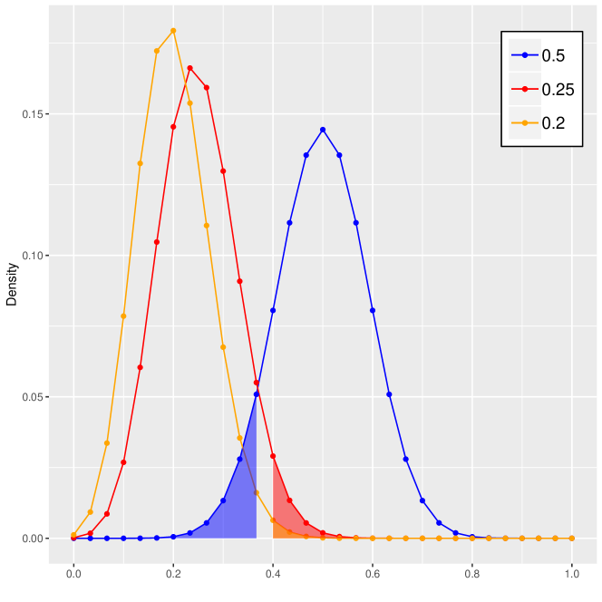
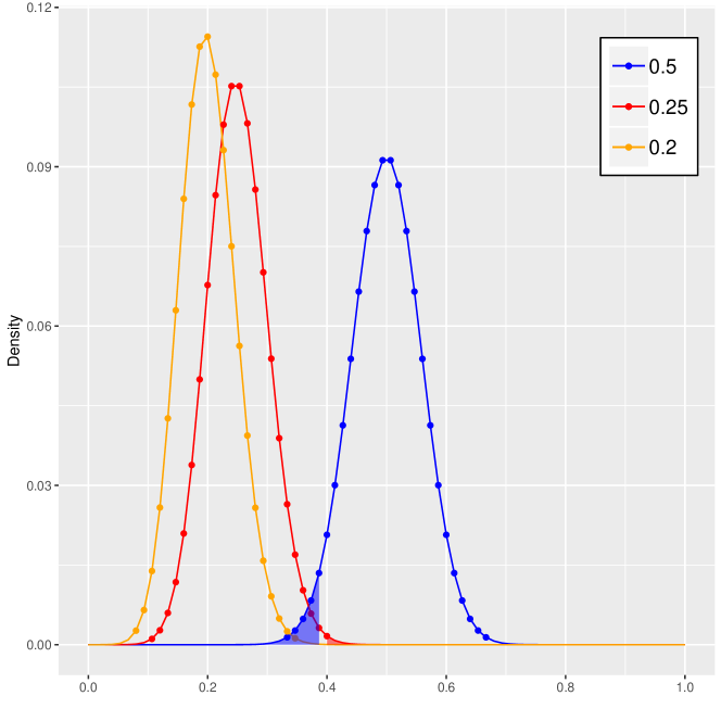
Figure 7: Continuous representation of the probability mass function of Binomial distributions. On the left we set $w=30$ and $q=0.4$, on the right $w=75$ and $q=0.4$, for both the probability of success (observing a negative gradient coherence) is $p\in\{0.2,0.25,0.5\}$. When $p=0.5$ (stationarity) the type I error happens with probability approximated by the shaded blue region. When $p<0.5$ (non stationarity) we erroneously declare stationarity with probability approximated by the shaded red and orange region.

For the experiments in the convex setting we use a feature matrix $X\in\mathbb{R}^{n\times d}$ with standard normal entries and $n=1000$, $d=20$. We set $\theta^{*}_{j}=5\cdot e^{-j/2}$ for $j=1,...,20$ to guarantee some difference in the entries. We generate the linear data as $y_{i}=X_{i}\cdot\theta^{*}+\epsilon_{i}$, where $\epsilon_{i}\sim N(0,1)$, and the data for logistic regression from a Bernoulli with probability $(1+e^{-X_{i}\cdot\theta^{*}})^{-1}$. The other parameters that are used through all Section 4.1 are the numbers of windows $w=20$ of size $l=50$ (so that each diagnostic consists of one epoch), the length of the first single thread $t_{1}=4$ epochs, and the acceptance proportion $q=0.4$.

As we say in the main text, in general we would like $w,l,t_{1}$ and the number of diagnostics $B$ to be as large as possible, given the computational budget that we have. The tolerance $q$, instead, is more tricky. In Theorem 2 and Figure 3 we shown that, as $t_{1}\to\infty$, the distribution of the sign of the gradient coherence is approximately a coin flip, provided that $\eta$ is small enough. This means that, once stationarity is reached, we want $q$ not to be too big, so that we will not observe a proportion of negative gradient coherences smaller than $q$ just by chance too often (and erroneously think that stationarity has not been reached yet). If we were then to assume independence between the $Q_{i}$, we should set $q$ to control the probability of a type I error (returning $T_{D}=N$ even though stationarity has been reached), which is

$$\frac{1}{2^{w}}\sum_{i=0}^{\lfloor w\cdot q\rfloor-1}\binom{w}{i}$$

However, if we set $q$ to be too small, then in the initial phases of the procedure we might think that we have already reached stationarity only because by chance we observed a proportion of negative dot products larger than $q$. This trade-off, represented in Figure 7, is particularly relevant if we cannot afford a large number of windows $w$, but it loses importance as $w$ grows.

E.2 Comparison with pflug Diagnostic with different parameters

In Figure 8 and Figure 9 we see other configurations for the experiment reported in the left panels of Figure 4. There, the starting point was set to be around $\theta_{s}$, where $\theta_{s,j}=5\cdot e^{-(d-j)/2}$ for $j=1,...,20$. Here we consider the same starting point for the panels on the right (for both linear and logistic regression) but a smaller learning rate. In both cases it is extremely clear that the pflug Diagnostic is detecting stationarity too late, and often (in the case of linear regression) running to the end of the budget. This can be a big problem in practice, because after stationarity has been reached all the iterations that keep using the same learning rate are not going to improve convergence, and are fundamentally wasted. In the left and middle panel of both figures we consider a starting point for the procedures around the minimizer $\theta^{*}$. In this scenario, for both larger and smaller learning rates, we see that both procedure are either very precise or detect stationarity a bit too early. This is a smaller problem in practice, since at that point the learning rate is reduced but the SGD procedures keep running, even if with a smaller learning rate. The speed of convergence is then slower, but the steps that we make are still important towards convergence.

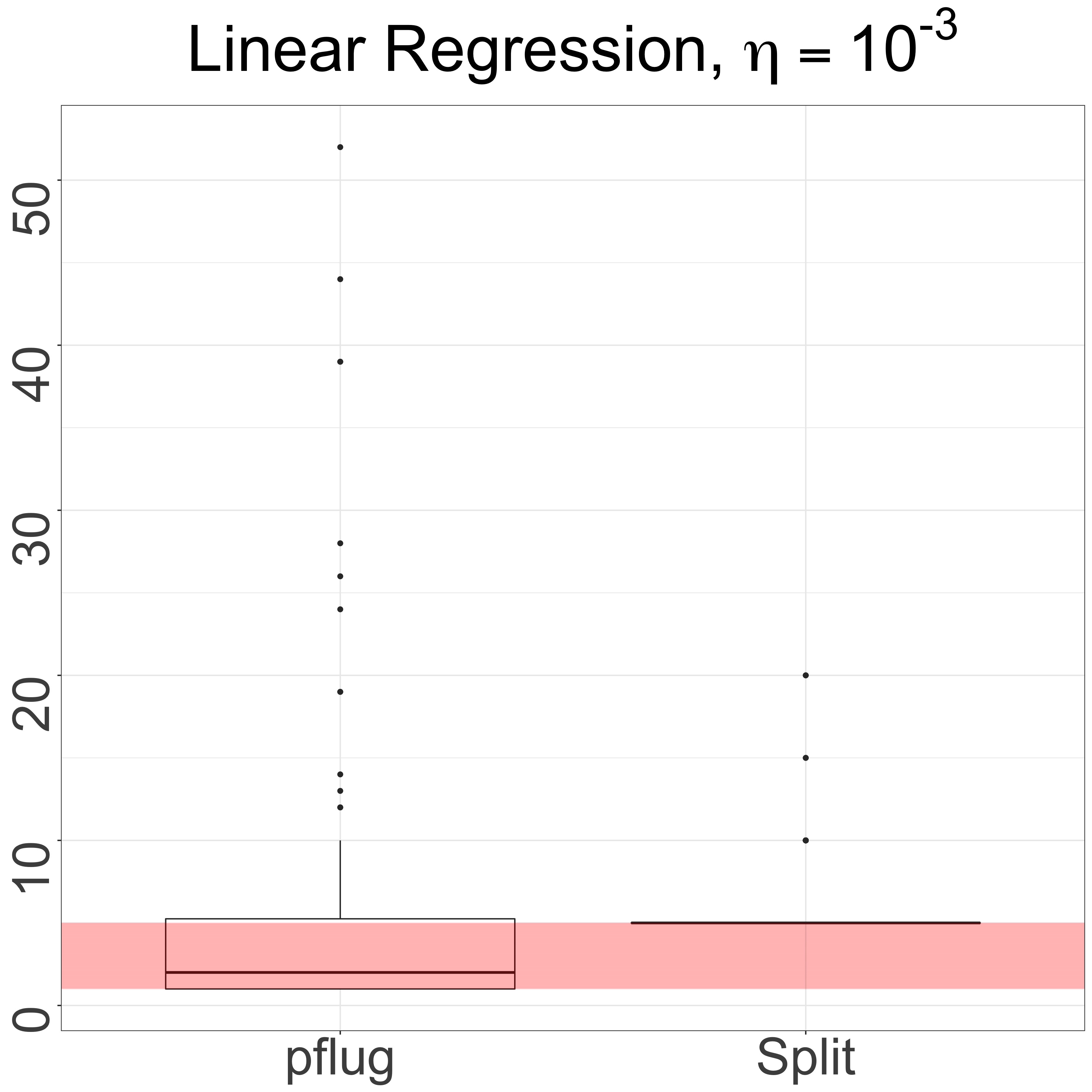
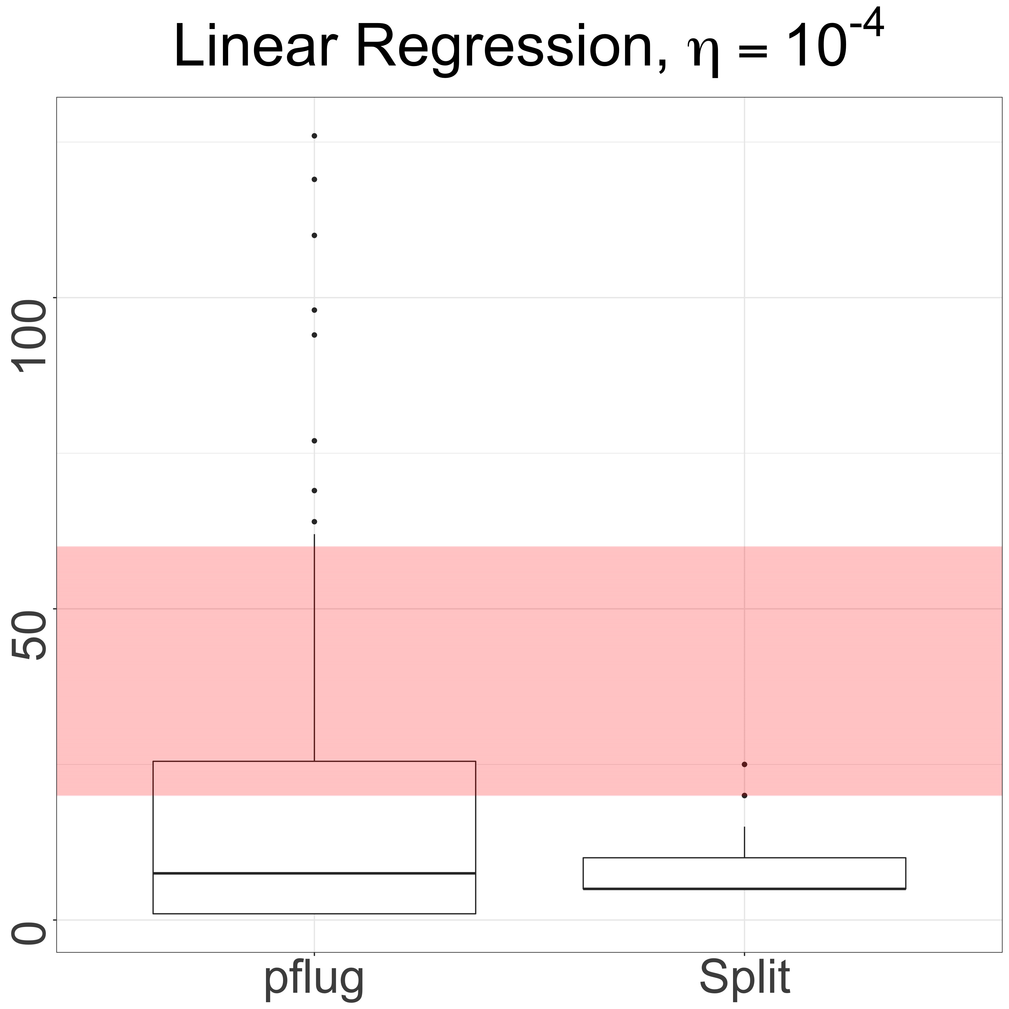
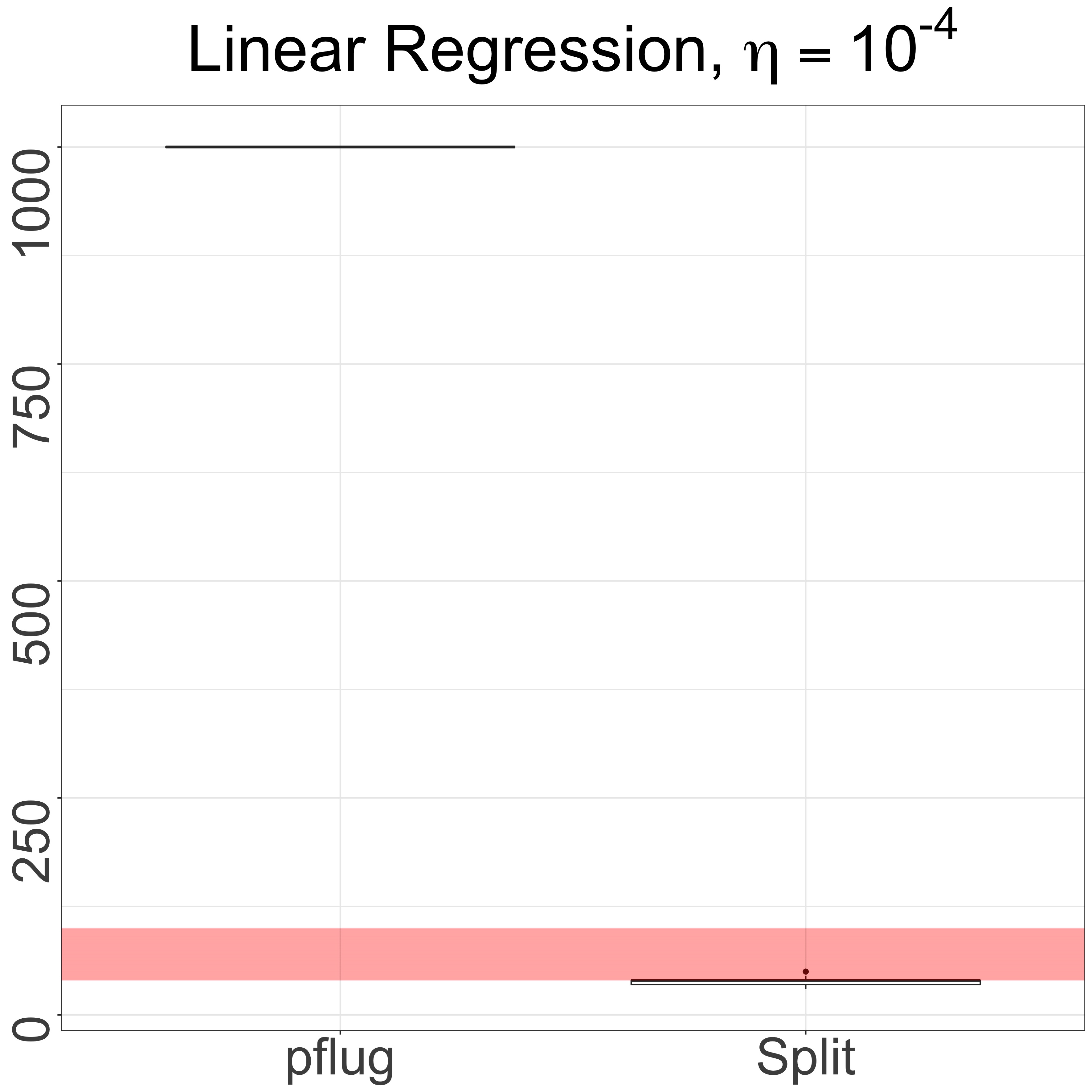
Figure 8: (left) starting around $\theta^{*}$, large learning rate. (middle) starting around $\theta^{*}$, small learning rate. (right) starting around $\theta_{s}$, small learning rate.

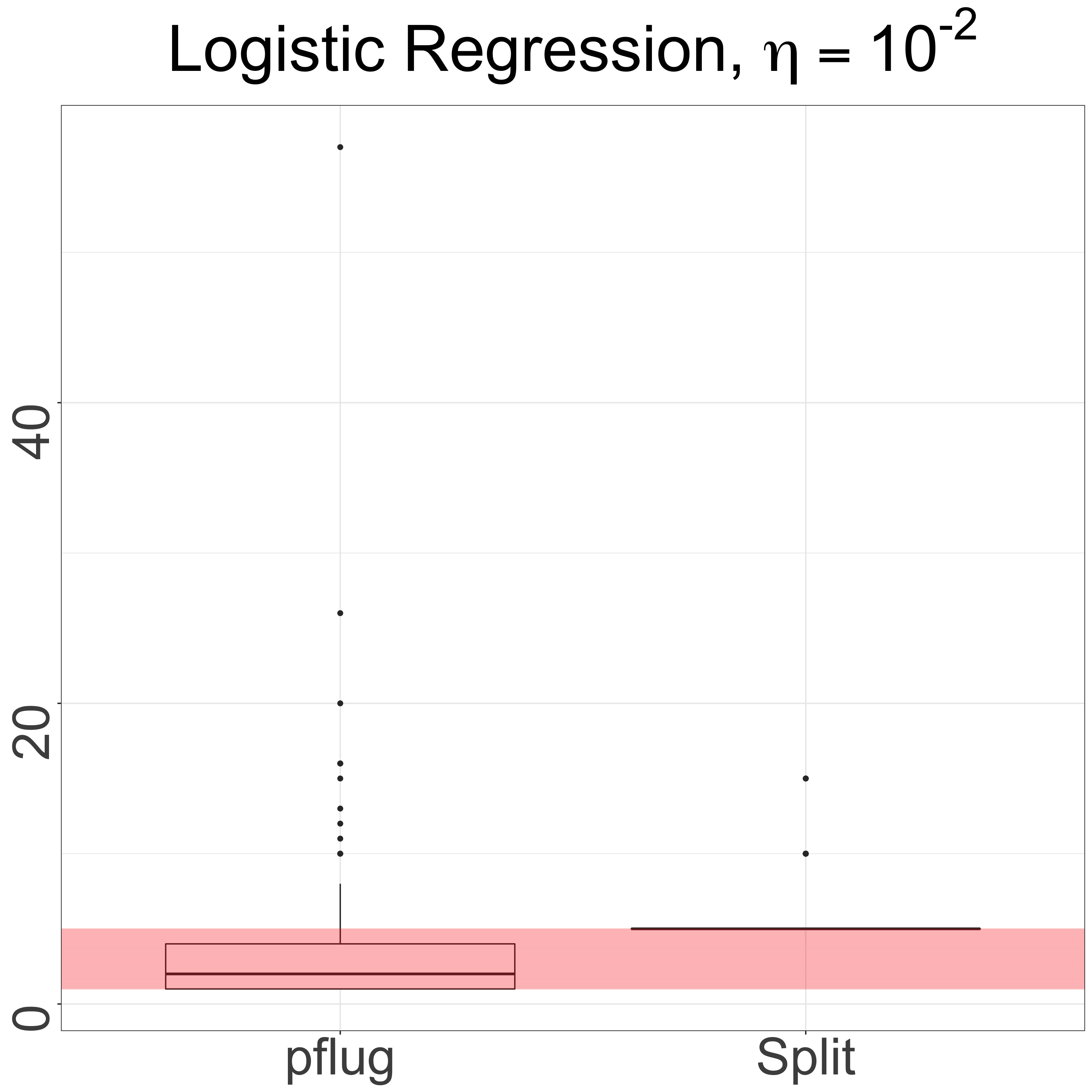
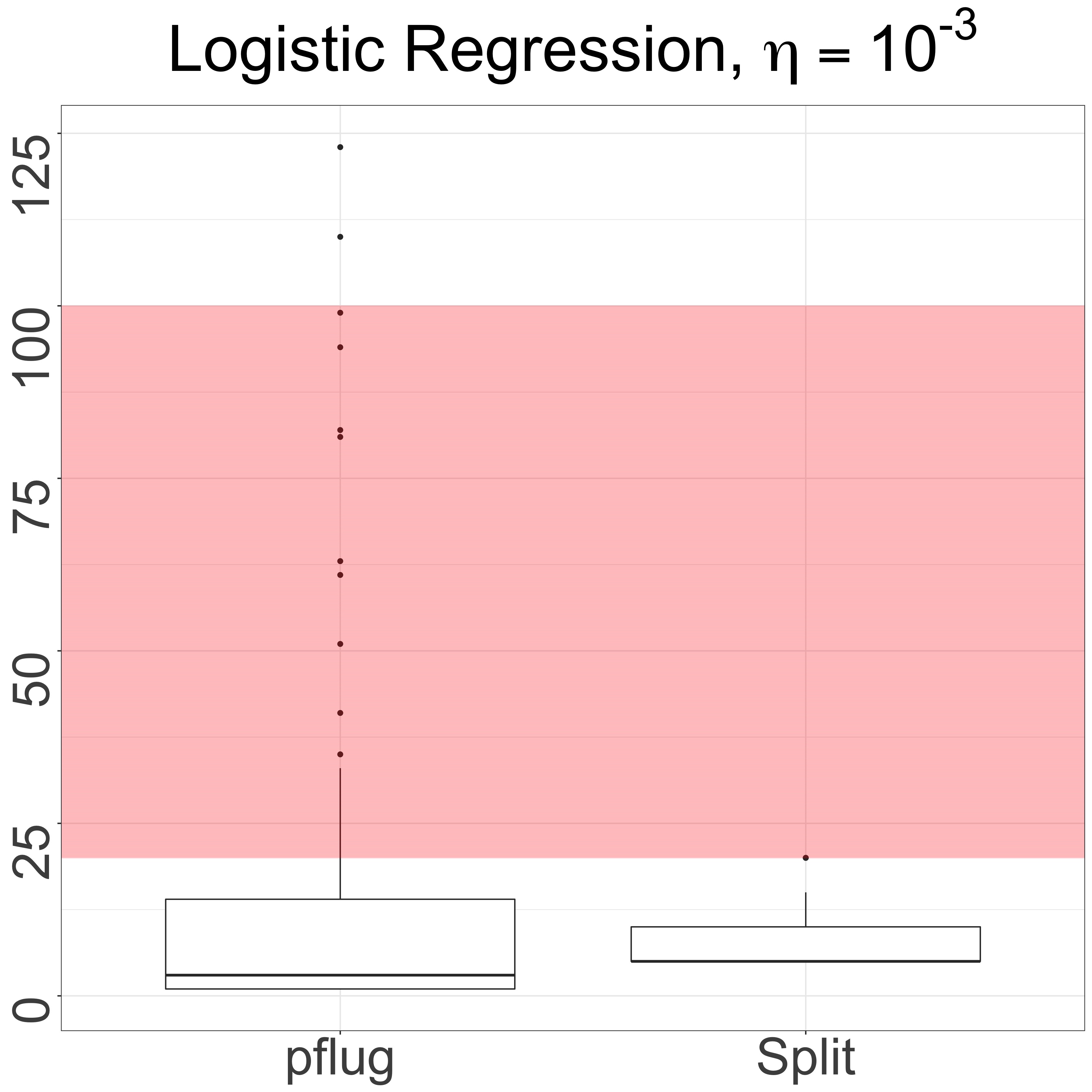
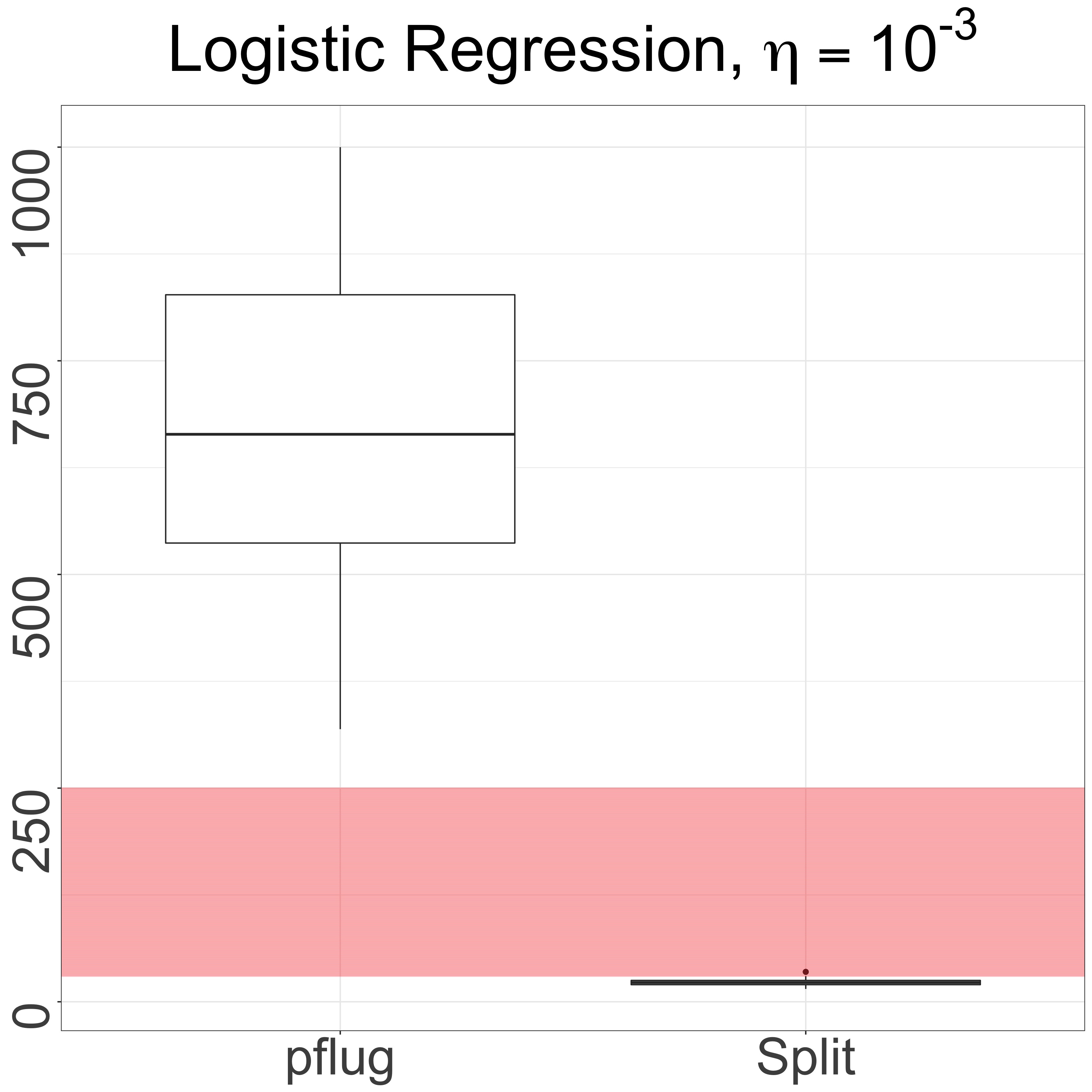
Figure 9: (left) starting around $\theta^{*}$, large learning rate. (middle) starting around $\theta^{*}$, small learning rate. (right) starting around $\theta_{s}$, small learning rate.

E.3 Another experiment in deep learning

When training the neural network VGG19 on CIFAR-10, we observe a similar behavior to what already shown in the third panel of Figure 5. SplitSGD, with both learning rates $110-1$ and $110-2$ achieves the same test accuracy of the manually tuned SGD, but in less epochs, and beats the performance of SGD and Adam. Also here it is possible to see the spikes given by the averaging, followed by the smoothing caused by the learning rate decay.

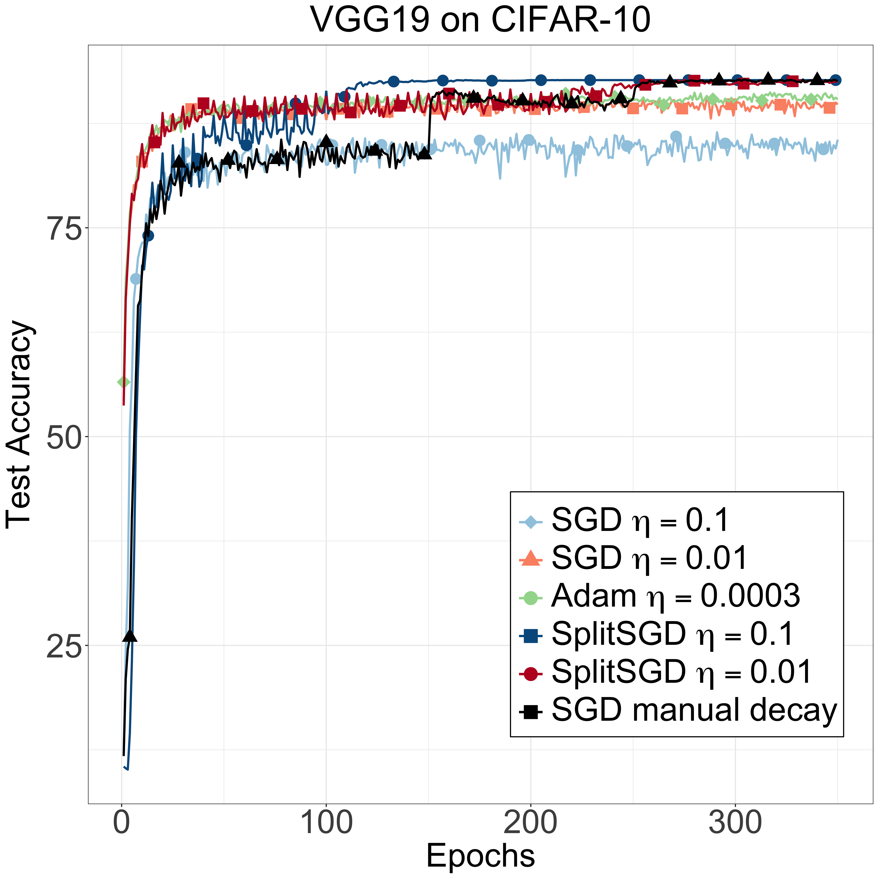
Figure 10: Compare the accuracy of SGD, Adam and SplitSGD in training VGG19 on CIFAR-10.

References

- Balles and Hennig, (2017) Balles, L. and Hennig, P. (2017). Dissecting adam: The sign, magnitude and variance of stochastic gradients. arXiv preprint arXiv:1705.07774.
- Balles et al., (2016) Balles, L., Romero, J., and Hennig, P. (2016). Coupling adaptive batch sizes with learning rates. arXiv preprint arXiv:1612.05086.
- Bengio, (2012) Bengio, Y. (2012). Practical recommendations for gradient-based training of deep architectures. In Neural networks: Tricks of the trade, pages 437–478. Springer.
- Bottou et al., (2018) Bottou, L., Curtis, F. E., and Nocedal, J. (2018). Optimization methods for large-scale machine learning. Siam Review, 60(2):223–311.
- Byrd et al., (2012) Byrd, R. H., Chin, G. M., Nocedal, J., and Wu, Y. (2012). Sample size selection in optimization methods for machine learning. Mathematical programming, 134(1):127–155.
- Chee and Toulis, (2018) Chee, J. and Toulis, P. (2018). Convergence diagnostics for stochastic gradient descent with constant learning rate. In Proceedings of the Twenty-First International Conference on Artificial Intelligence and Statistics, volume 84 of Proceedings of Machine Learning Research, pages 1476–1485. PMLR.
- Dauphin et al., (2015) Dauphin, Y., De Vries, H., and Bengio, Y. (2015). Equilibrated adaptive learning rates for non-convex optimization. In Advances in neural information processing systems, pages 1504–1512.
- De et al., (2017) De, S., Yadav, A., Jacobs, D., and Goldstein, T. (2017). Automated inference with adaptive batches. In Artificial Intelligence and Statistics, pages 1504–1513.
- Delyon and Juditsky, (1993) Delyon, B. and Juditsky, A. (1993). Accelerated stochastic approximation. SIAM Journal on Optimization, 3(4):868–881.
- Duchi et al., (2011) Duchi, J., Hazan, E., and Singer, Y. (2011). Adaptive subgradient methods for online learning and stochastic optimization. Journal of Machine Learning Research, 12(Jul):2121–2159.
- Hochreiter and Schmidhuber, (1997) Hochreiter, S. and Schmidhuber, J. (1997). Long short-term memory. Neural computation, 9(8):1735–1780.
- Keskar et al., (2016) Keskar, N. S., Mudigere, D., Nocedal, J., Smelyanskiy, M., and Tang, P. T. P. (2016). On large-batch training for deep learning: Generalization gap and sharp minima. arXiv preprint arXiv:1609.04836.
- Keskar and Socher, (2017) Keskar, N. S. and Socher, R. (2017). Improving generalization performance by switching from adam to sgd. arXiv preprint arXiv:1712.07628.
- Kingma and Ba, (2014) Kingma, D. P. and Ba, J. (2014). Adam: A method for stochastic optimization. arXiv preprint arXiv:1412.6980.
- Krizhevsky et al., (2009) Krizhevsky, A., Hinton, G., et al. (2009). Learning multiple layers of features from tiny images. Technical report, Citeseer.
- Lang et al., (2019) Lang, H., Zhang, P., and Xiao, L. (2019). Using statistics to automate stochastic optimization. arXiv preprint arXiv:1909.09785.
- Le Roux et al., (2013) Le Roux, N., Schmidt, M. W., and Bach, F. R. (2013). A stochastic gradient method with an exponential convergence rate for finite training sets. Advances in Neural Information Processing Systems, 25:3–6.
- Li et al., (2017) Li, C. J., Li, L., Qian, J., and Liu, J.-G. (2017). Batch size matters: A diffusion approximation framework on nonconvex stochastic gradient descent. stat, 1050:22.
- Li et al., (2014) Li, M., Zhang, T., Chen, Y., and Smola, A. J. (2014). Efficient mini-batch training for stochastic optimization. In Proceedings of the 20th ACM SIGKDD international conference on Knowledge discovery and data mining, pages 661–670. ACM.
- Luo et al., (2019) Luo, L., Xiong, Y., Liu, Y., and Sun, X. (2019). Adaptive gradient methods with dynamic bound of learning rate. arXiv preprint arXiv:1902.09843.
- Marcus et al., (1993) Marcus, M., Santorini, B., and Marcinkiewicz, M. A. (1993). Building a large annotated corpus of english: The penn treebank.
- McCandlish et al., (2018) McCandlish, S., Kaplan, J., Amodei, D., and Team, O. D. (2018). An empirical model of large-batch training. arXiv preprint arXiv:1812.06162.
- Moulines and Bach, (2011) Moulines, E. and Bach, F. R. (2011). Non-asymptotic analysis of stochastic approximation algorithms for machine learning. In Advances in Neural Information Processing Systems, pages 451–459.
- Murata, (1998) Murata, N. (1998). A statistical study of on-line learning. Online Learning and Neural Networks. Cambridge University Press, Cambridge, UK, pages 63–92.
- Pflug, (1990) Pflug, G. C. (1990). Non-asymptotic confidence bounds for stochastic approximation algorithms with constant step size. Monatshefte für Mathematik, 110(3-4):297–314.
- Polyak and Juditsky, (1992) Polyak, B. T. and Juditsky, A. B. (1992). Acceleration of stochastic approximation by averaging. SIAM Journal on Control and Optimization, 30(4):838–855.
- Qian, (1999) Qian, N. (1999). On the momentum term in gradient descent learning algorithms. Neural networks, 12(1):145–151.
- Robbins and Monro, (1951) Robbins, H. and Monro, S. (1951). A stochastic approximation method. The annals of mathematical statistics, pages 400–407.
- Ruppert, (1988) Ruppert, D. (1988). Efficient estimations from a slowly convergent Robbins–Monro process. Technical report, Operations Research and Industrial Engineering, Cornell University, Ithaca, NY.
- Smith et al., (2017) Smith, S. L., Kindermans, P.-J., Ying, C., and Le, Q. V. (2017). Don’t decay the learning rate, increase the batch size. arXiv preprint arXiv:1711.00489.
- Su and Zhu, (2018) Su, W. J. and Zhu, Y. (2018). Uncertainty quantification for online learning and stochastic approximation via hierarchical incremental gradient descent. arXiv preprint arXiv:1802.04876.
- Sutskever et al., (2013) Sutskever, I., Martens, J., Dahl, G., and Hinton, G. (2013). On the importance of initialization and momentum in deep learning. In International conference on machine learning, pages 1139–1147.
- Tan et al., (2016) Tan, C., Ma, S., Dai, Y.-H., and Qian, Y. (2016). Barzilai-borwein step size for stochastic gradient descent. In Advances in Neural Information Processing Systems, pages 685–693.
- Xiao et al., (2017) Xiao, H., Rasul, K., and Vollgraf, R. (2017). Fashion-mnist: a novel image dataset for benchmarking machine learning algorithms. arXiv preprint arXiv:1708.07747.
- Yaida, (2019) Yaida, S. (2019). Fluctuation-dissipation relations for stochastic gradient descent. In ICLR.
- Yin et al., (2017) Yin, D., Pananjady, A., Lam, M., Papailiopoulos, D., Ramchandran, K., and Bartlett, P. (2017). Gradient diversity: a key ingredient for scalable distributed learning. arXiv preprint arXiv:1706.05699.
- Yin, (1989) Yin, G. (1989). Stopping times for stochastic approximation. In Modern Optimal Control: A Conference in Honor of Solomon Lefschetz and Joseph P. LaSalle, pages 409–420.
- Zhang and Mitliagkas, (2017) Zhang, J. and Mitliagkas, I. (2017). Yellowfin and the art of momentum tuning. arXiv preprint arXiv:1706.03471.