Acceleration techniques for semiclassical Maxwell-Bloch systems: An application to discrete quantum dot ensembles

Abstract

The solution to Maxwell-Bloch systems using an integral-equation-based framework has proven effective at capturing collective features of laser-driven and radiation-coupled quantum dots, such as light localization and modifications of Rabi oscillations [1]. Importantly, it enables observation of the dynamics of each quantum dot in large ensembles in a rigorous, error-controlled, and self-consistent way without resorting to spatial averaging. Indeed, this approach has demonstrated convergence in ensembles containing up to $10^{4}$ interacting quantum dots [1]. Scaling beyond $10^{4}$ quantum dots tests the limit of computational horsepower, however, due to the $\mathcal{O}(N_{t}N_{s}^{2})$ scaling (where $N_{t}$ and $N_{s}$ denote the number of temporal and spatial degrees of freedom). In this work, we present an algorithm that reduces the cost of analysis to $\mathcal{O}(N_{t}N_{s}\log^{2}N_{s})$. While the foundations of this approach rely on well-known particle-particle/particle-mesh and adaptive integral methods, we add refinements specific to transient systems and systems with multiple spatial and temporal derivatives. Accordingly, we offer numerical results that validate the accuracy, effectiveness and utility of this approach in analyzing the dynamics of large ensembles of quantum dots.

1 Introduction

The computational simulation of the nonlinear propagation of laser pulses through materials presents formidable challenges, particularly in materials containing dispersed quantum dots or nanoparticles that have strong light-matter coupling. One phenomenon, Rabi oscillations, demonstrates nonlinear behavior that can arise from such coupling. These oscillations have a long history of study in single quantum dots [2, 3, 4], though understanding the collective Rabi dynamics of quantum dot ensembles requires a careful analysis of emission effects that couple quantum dots to produce many-body collective effects. Researchers have a significant interest in examining these effects from theoretical, numerical, and experimental perspectives [5, 6, 1, 7]. For instance, experiments on novel systems based on perovskite nanocrystals have recently demonstrated these effects [8]. These experiments could lead to novel composite materials with enhanced optical properties.

Typical theoretical and computational analyses use variations of the Maxwell-Bloch equations [9] to describe the collective behavior of ensembles of optically active centers in which classical radiation fields couple a quantum description of each center. To this end, methods such as homogenization [10, 11], differential-equation-based methods [12, 13, 14, 15, 16], and, more recently, integral-equation-based methods [1] all describe the dynamics of coupled quantum dot systems, each with a differing level of fidelity.

Approaches that do not rely on homogenization use coupled discrete methods to solve the classical Maxwell equations and local time evolution techniques to solve the Bloch equations for each quantum dot. Spatial homogenization, on the other hand, describes the near and far radiation characteristics of a quantum dot assuming homogeneous background material properties [17]. This approach has limited validity as it does not account for strong interactions between particles in each other’s nearfield, a shortcoming exacerbated by the non-linear regimes considered here. Differential equation methods [18] to solve the Maxwell system have included finite-difference, time-domain finite-element, and discontinuous Galerkin methods, though all succumb to various numerical inaccuracies due to the nature of discretization. The inaccuracies most pertinent to simulation of quantum dot systems extend from the need to include point dipole sources in the simulation and capture near field effects that behave as $1/r^{3}$ (where $r$ denotes the distance between centers). Accurately recovering these fields has numerous challenges and one needs dense discretization in the vicinity of dots together with equivalent/soft sources to accurately capture these effects [15]. Additionally, static null spaces that grow linearly with time present another challenge with conventional time-domain finite-element techniques [18]. On the plus side, these methods offer a high degree of flexibility and can accommodate different background linear bulk materials.

Our approach [1] differs significantly. We make use of an integral equation-based formulation that employs a retarded potential to compute fields radiated by every quantum dot. This approach does not rely on a particular discretization and only depends on the number of quantum dots under investigation. Demonstrations of the accuracy of this approach appear in [1], though this method faces a fundamental bottleneck: both the memory necessary and computational cost scale as $\mathcal{O}(N_{t}N_{s}^{2})$ which becomes prohibitive for extended ensembles. A traditional acceleration technique that readily adapts to these equations makes use of a rotated frame approximation to reduce the number of timesteps by a factor of $\sim\!1000$. This approximation exploits the narrowband nature of the nonlinearity which enables the use of envelope functions [16]. Physically, this arises due to the large difference between the characteristic Rabi energy associated with light-matter coupling and the optical transition energy. Computationally, this enables timestep sizes much larger than the inverse of the laser frequency. While this approximation offers significant acceleration, the key bottleneck IS the cost of evaluating retarded potentials, which scales quadratically with the number of quantum dots; thankfully, there exists extensive literature on reducing this cost that we examine next.

Two algorithms typically see use in accelerating the evaluation of retarded potentials: the Plane-Wave Time-Domain method (PWTD) and the Adaptive Integral Method (AIM, a variation of particle-particle/particle-mesh techniques) [19, 20]. Unfortunately, neither of these methods apply directly to the problem at hand. To set the stage for discussion, assume that one needs to evaluate the radiated electric field $\mathbf{E}_{R}(\mathbf{r},t)=\mathfrak{F}\{\mathbf{P}(\mathbf{r},t)\}$ [21] due to a polarization density $\mathbf{P}(\mathbf{r},t)$ via $\mathfrak{F}\{\mathbf{P}(\mathbf{r},t)\}=\mathcal{L}\quantity{g(\mathbf{r},t)}\star_{st}\mathbf{P}(\mathbf{r},t)$ where $g(\mathbf{r},t)=\delta(t-|\mathbf{r}|/c)/(4\pi|\mathbf{r}|)$ denotes the retarded potential, $\mathcal{L}\quantity{g(\mathbf{r},t)}=-\mu_{0}\quantity(\partial_{t}^{2}\mathrm{I}\cdot-c^{2}\nabla\nabla\cdot)g(\mathbf{r},t)$ denotes a dyadic differential operator, and $\mathrm{I}$ denotes the identity dyad.

PWTD exploits the properties of radiated fields due to quiescent sources that occupy a bounded spatial domain. These fields have a bandlimit (in momentum space) that PWTD leverages to reconstruct them to arbitrary precision using a tree-based approach; see [19] and references therein. However, the crux of this methodology lies in the fact that spatial variation scales with the temporal one (times $c$). Unfortunately, while this holds in the fixed frame, it does not in the rotated frame.

AIM, on the other hand, relies on moments around a uniform grid (independent of temporal variation) to reconstruct sources and their resulting field distributions. This idea—using grids for computing translationally-invariant functions by exploiting an underlying block Toeplitz structure—has seen extensive use in molecular dynamics simulations to evaluate Laplace, Helmholtz, and wave equation kernels [22, 20, 23]. In all these cases, one evaluates the space (and time) convolution with a scalar quantity, sans the operator $\mathcal{L}\quantity{\cdot}$ required herein. Unfortunately, the nature of $\mathcal{L}\quantity{\cdot}$ determines the number of potentials that need evaluation. As we will see in the ensuing sections, the $\mathcal{L}\quantity{\cdot}$ used for quantum dots contains numerous dyadic terms, each with different orders of temporal derivatives. As a result, a naïve application of AIM to each term of the expression quickly becomes untenable and we seek to develop a more expedient technique.

This paper has two principal contributions: (i) development and demonstration of techniques that overcome computational complexity (memory and CPU costs) associated with evaluation of integral equation operators, and (ii) demonstration of these algorithms to examine optical systems containing quantum dots. In developing these algorithms, we examine their runtime and accuracy and, more importantly, show that evaluating $\mathcal{L}\quantity{g(\mathbf{r},t)}$ incurs approximately the same cost as evaluating $g(\mathbf{r},t)$ albeit with lower error.

We organize the rest of this paper as follows: in section 2 we define the problem, and provide the means to a solution in section 3. Section 4 develops the AIM method for the Maxwell-Bloch problem and outlines its computational complexity. Next, in section 5, we present a number of results that verify the claims of accuracy, complexity, and applicability of this method to a collection of quantum dots. Finally, in section 6 we summarize the contributions of the paper and outline future research avenues.

2 Formulation

Consider a domain $\Omega$ that contains $N_{s}$ randomly distributed quantum dots. A time-varying electromagnetic field of central frequency $\omega$ impinges on $\Omega$ and excites each quantum dot. We wish to develop the means to study the evolution of these quantum dots in response to both the incident excitation as well as radiation produced by other quantum dots. Toward this end, we employ a semi-classical approach to understand the response of each quantum dot to the incident field that comprises the laser field as well as fields radiated by other dots (computed classically). In what follows, we provide a brief description of the requisite formulation for completeness; [1] provides a more detailed description.

Dipolar transitions govern the response of each quantum dot to the exciting field. Specifically, we write the time-dependence of a given quantum dot’s density matrix, $\hat{\rho}(t)$, as

$$\derivative{\hat{\rho}}{t}=\frac{-i}{\hbar}\commutator{\hat{\mathcal{H}}(t)}{\hat{\rho}}-\hat{\mathcal{D}}\quantity[\hat{\rho}].$$ (1)

For two-level systems, $\hat{\rho}(t)$ denotes a two by two matrix with three unique unknowns ($\rho_{00}$ and the real and imaginary parts of $\rho_{01}$), $\hat{\mathcal{H}}(t)$ represents a local Hamiltonian that governs the internal two-level structure of the quantum dot as well as its interaction with an external electromagnetic field, and $\hat{\mathcal{D}}$ provides dissipation terms that account for spontaneous emission effects phenomenologically. Explicitly,

where $\chi(t)\equiv\mathbf{d}\cdot\hat{\mathbf{E}}(\mathbf{r},t)/\hbar$, $\mathbf{d}\equiv\matrixelement{1}{e\hat{\mathbf{r}}}{0}$, and the kets represent the highest valence and lowest conduction states of the quantum dot under consideration. Finally, the $T_{1}$ and $T_{2}$ constants characterize average relaxation and decoherence times.

We compute the semi-classical interaction between quantum dots assuming coherent fields and negligible quantum statistical effects. Such assumptions imply classical electromagnetic interactions while preserving the two-level structure of individual quantum dots. To this end, we write the total electric field at any point in space and time as $\mathbf{E}(\mathbf{r},t)=\mathbf{E}_{L}(\mathbf{r},t)+\mathfrak{F}\{\mathbf{P}(\mathbf{r},t)\}$ where $\mathbf{E}_{L}(\mathbf{r},t)$ denotes the incident laser field, $\mathbf{P}(\mathbf{r},t)$ gives a polarization distribution arising from the off-diagonal elements (coherences) of $\hat{\rho}$, and

$$\begin{split}\mathfrak{F}\{\mathbf{P}(\mathbf{r},t)\}&\doteq-\mu_{0}\quantity(\partial^{2}_{t}\mathrm{I}-c^{2}\nabla\nabla)g\quantity(\mathbf{r},t)\star_{st}\mathbf{P}\quantity(\mathbf{r},t)\\ &\doteq\frac{-1}{4\pi\epsilon}\int\left(\mathrm{I}-\bar{\mathbf{r}}\!\otimes\!\bar{\mathbf{r}}\right)\cdot\frac{\partial_{t}^{2}\mathbf{P}(\mathbf{r}^{\prime},t_{R})}{c^{2}\absolutevalue{\mathbf{r}-\mathbf{r}^{\prime}}}+\left(\mathrm{I}-3\bar{\mathbf{r}}\!\otimes\!\bar{\mathbf{r}}\right)\cdot\quantity(\frac{\partial_{t}\mathbf{P}(\mathbf{r}^{\prime},t_{R})}{c\absolutevalue{\mathbf{r}-\mathbf{r}^{\prime}}^{2}}+\frac{\mathbf{P}(\mathbf{r}^{\prime},t_{R})}{\absolutevalue{\mathbf{r}-\mathbf{r}^{\prime}}^{3}})\differential[3]{\mathbf{r}^{\prime}}\end{split}$$ (2c)

(see [24, section §72]). In the above expression, $\bar{\mathbf{r}}\equiv\quantity(\mathbf{r}-\mathbf{r}^{\prime})/\absolutevalue{\mathbf{r}-\mathbf{r}^{\prime}}$, $\otimes$ represents the tensor product (i.e. $\quantity(\mathbf{a}\!\otimes\!\mathbf{b})_{ij}=a_{i}b_{j}$), $t_{R}\equiv t-\absolutevalue{\mathbf{r}-\mathbf{r}^{\prime}}/c$, and $\epsilon$ gives the dielectric constant of the inter-dot medium. Thus, in a system composed of multiple quantum dots, eq. 2c couples the evolution of each quantum dot by way of the off-diagonal matrix elements appearing in LABEL:eq:hamiltonian.

Note that this approach does not require an instantaneous dipole-dipole Coulomb term between (charge-neutral) quantum dots; the interactions between structures occur only via the electric field which propagates through space with finite velocity (see  [25, sections A${}_{\textsc{iv}}$ and C${}_{\textsc{iv}}$] for in-depth discussions of this point).

In the systems under consideration here, $\omega_{0}$ lies in the optical frequency band ($\sim$1500\text{\,}\mathrm{m}\mathrm{eV}\mathrm{/}\hbar$$). Consequently, integrating eq. 1 directly to resolve the Rabi dynamics that occur on the order of $1\text{\,}\mathrm{ps}$ quickly becomes computationally infeasible. Introducing $\tilde{\rho}=\hat{U}\hat{\rho}\hat{U}^{\dagger}$ where $\hat{U}=\mathrm{diag}(1,e^{i\omega t})$, we may instead write eq. 1 as

$$\derivative{\tilde{\rho}}{t}=\frac{-i}{\hbar}\commutator{\hat{U}\hat{\mathcal{H}}\hat{U}^{\dagger}-i\hbar\hat{V}}{\tilde{\rho}}-\hat{\mathcal{D}}\quantity[\tilde{\rho}],\quad\hat{V}\equiv\hat{U}\derivative{\hat{U}^{\dagger}}{t}$$ (2d)

which contains only terms proportional to $e^{i(\omega_{0}\pm\omega)t}$ if $\mathbf{E}(t)\sim\tilde{\mathbf{E}}(t)\cos(\omega t)$. Consequently, we ignore the high-frequency quantities (corresponding to $\omega_{0}+\omega$) under the assumption that such terms will integrate to zero in solving eq. 2d over appreciable timescales [26]. One can then construct efficient numerical strategies for solving eq. 2d. A similar transformation applies to the source distribution $\mathbf{P}(\mathbf{r},t)$; by assuming $\mathbf{P}(\mathbf{r},t)=\tilde{\mathbf{P}}(\mathbf{r},t)e^{i\omega t}$ in eq. 2c the radiated field envelope becomes

$$\begin{gathered}\tilde{\mathfrak{F}}\{\tilde{\mathbf{P}}(\mathbf{r},t)\}\equiv\frac{-1}{4\pi\epsilon}\int\quantity(\mathrm{I}-\bar{\mathbf{r}}\!\otimes\!\bar{\mathbf{r}})\cdot\frac{\quantity(\partial_{t}^{2}\tilde{\mathbf{P}}(\mathbf{r}^{\prime},t_{R})+2i\omega\partial_{t}\tilde{\mathbf{P}}(\mathbf{r}^{\prime},t_{R})-\omega^{2}\tilde{\mathbf{P}}(\mathbf{r}^{\prime},t_{R}))e^{-i\omega\absolutevalue{\mathbf{r}-\mathbf{r}^{\prime}}/c}}{c^{2}\absolutevalue{\mathbf{r}-\mathbf{r}^{\prime}}}+\\ \quantity(\mathrm{I}-3\bar{\mathbf{r}}\!\otimes\!\bar{\mathbf{r}})\cdot\frac{\quantity(\partial_{t}\tilde{\mathbf{P}}(\mathbf{r}^{\prime},t_{R})+i\omega\tilde{\mathbf{P}}(\mathbf{r}^{\prime},t_{R}))e^{-i\omega\absolutevalue{\mathbf{r}-\mathbf{r}^{\prime}}/c}}{c\absolutevalue{\mathbf{r}-\mathbf{r}^{\prime}}^{2}}+\quantity(\mathrm{I}-3\bar{\mathbf{r}}\!\otimes\!\bar{\mathbf{r}})\cdot\frac{\tilde{\mathbf{P}}(\mathbf{r}^{\prime},t_{R})e^{-i\omega\absolutevalue{\mathbf{r}-\mathbf{r}^{\prime}}/c}}{\absolutevalue{\mathbf{r}-\mathbf{r}^{\prime}}^{3}}\,\differential[3]{\mathbf{r}^{\prime}}.\end{gathered}$$ (2g)

Note that eq. 2g maintains the high-frequency phase relationship between sources oscillating at $\omega$ via the factors of $e^{-i\omega\absolutevalue{\mathbf{r}-\mathbf{r}^{\prime}}/c}$ that appear. As a result, we write

$$\tilde{\mathbf{E}}(\mathbf{r},t)=\tilde{\mathbf{E}}_{L}(\mathbf{r},t)+\tilde{\mathfrak{F}}\{\tilde{\mathbf{P}}(\mathbf{r},t)\}$$ (2h)

and the evolution of the ensemble relies on a self-consistent solution of eqs. 2d and 2h. As evident from eq. 2g, this comprises a large number of costly potential integrals arising from the number of dyadic components and number of time derivatives. As such, we now turn our attention to an efficient computational infrastructure for ameliorating this cost.

3 Discrete Solution

Solving eqs. 2d and 2h self-consistently proceeds via the following steps: (i) represent the time varying behavior of the polarization (ii) using (2h), evaluate $\tilde{\mathbf{E}}(\mathbf{r},t)$ at a given timestep, and (iii) use a predictor corrector approach to evaluate $\tilde{\rho}$ via (2d). Representing $\tilde{\mathbf{P}}(\mathbf{r},t)$ in terms of space and time basis functions such that

$$\tilde{\mathbf{P}}(\mathbf{r},t)\approx\sum_{\ell=0}^{N_{s}-1}\sum_{m=0}^{N_{t}-1}\tilde{\mathcal{A}}_{\ell}^{(m)}\mathbf{s}_{\ell}(\mathbf{r})T(t-m\,\Delta t),$$ (2i)

$\tilde{\mathcal{A}}_{\ell}^{(m)}=\tilde{\rho}_{\ell,01}(m\,\Delta t)$ gives the polarization associated with the $\ell$th quantum dot at the $m$th time step, and $\Delta t$ denotes a fixed time interval chosen to accurately sample the dynamics of the physical quantities involved. Both $\mathbf{s}_{\ell}(\mathbf{r})$ and $T(t)$ have finite support and $T(t)$ obeys (discrete) causality (i.e. $T(t)=0$ if $t<-\Delta t$). In particular, we consider shifted Lagrange polynomials for the $T(t)$ and assume dipolar transitions in the quantum dots allowing for $\mathbf{s}_{\ell}(\mathbf{r})=\mathbf{d}_{\ell}\delta(\mathbf{r}-\mathbf{r}_{\ell})$, though this analysis readily extends to accommodate any similar set of functions [27, 28].

Substituting eq. 2i into eq. 2g and projecting the resulting fields onto $\delta(t-m\,\Delta t)\mathbf{s}_{\ell}(\mathbf{r})$, we obtain

$$\tilde{\mathcal{E}}^{(m)}=\tilde{\mathcal{E}}_{\text{inc}}^{(m)}+\sum_{m^{\prime}=0}^{m}\tilde{\mathcal{F}}^{(m-m^{\prime})}\boldsymbol{\cdot}\tilde{\mathcal{A}}^{(m^{\prime})}$$ (2j)

where

$$\tilde{\mathcal{E}}^{(m)} =\langle\mathbf{s}_{\ell}(\mathbf{r}),\,\tilde{\mathbf{E}}(\mathbf{r},m\,\Delta t)\rangle$$ (2ka)

$$\tilde{\mathcal{E}}^{(m)}_{\text{inc},\ell} =\langle\mathbf{s}_{\ell}(\mathbf{r}),\,\tilde{\mathbf{E}}_{\text{inc}}(\mathbf{r},m\,\Delta t)\rangle$$ (2kb)

$$\tilde{\mathcal{F}}^{(k)}_{\ell\ell^{\prime}} =\big{\langle}\mathbf{s}_{\ell}(\mathbf{r}),\,\tilde{\mathfrak{F}}\quantity{\mathbf{s}_{\ell^{\prime}}(\mathbf{r})T(k\,\Delta t)}\big{\rangle}$$ (2kc)

and $\langle\cdot,\cdot\rangle$ denotes the inner product between functions.

A self-consistent solution to eqs. 2d and 2h then has the following prescription for any timestep: (i) predict $\tilde{\mathcal{A}}_{\ell}^{(m)}=\tilde{\rho}_{\ell,01}(m\,\Delta t)$ $\forall~{}\ell$ from the known prior history of the system, (ii) compute $\tilde{\mathcal{E}}^{(m)}_{\ell}$ using eq. 2j, (iii) find $\partial_{t}\,\tilde{\rho}_{\ell,01}(m\,\Delta t)$ using eq. 2d, and (iv) correct $\tilde{\rho}_{\ell,01}(m\,\Delta t)$ and iterate through steps (ii) through (iv) until converged.

The time complexity of the entire algorithm follows naturally from the above description: for $N_{s}$ particles and $N_{t}$ timesteps, the cost of evaluating eq. 2j scales as $\mathcal{O}(N_{t}N_{s}^{2})$ while the cost of solving eq. 2d for every quantum dot scales as $\mathcal{O}(N_{t}N_{s})$. As a result, the bottleneck arises from the discrete convolution/field evaluation at every timestep, and we address strategies to ameliorate this cost in the next section.

4 Acceleration via Fast Fourier Transforms

Figure 1: Illustration of the grid structure and related terminology. All of the sources within a box (shown as the central shaded square) map to the same set of expansion points (shown as open circles) indexed relative to $\mathbf{r}_{\text{box}}$.

As alluded to earlier, TD-AIM forms the basis our approach to reducing the computational complexity. Unfortunately, we cannot directly apply existing methodologies due to overhead induced by the multiplicity of terms as well as temporal derivatives. In what follows, we develop a variation of TD-AIM that relies on propagating the convolution of the retarded potential with the source function and local evaluation of spatial and temporal derivatives.

4.1 Algorithmic Details

In what follows, we give algorithmic steps for the fixed frame elements, $\mathcal{F}^{(k)}$. The algorithmic steps for the rotating wave elements, $\tilde{\mathcal{F}}^{(k)}$, proceed identically. To effect a sub-quadratic calculation of eq. 2j, we approximate $\mathcal{F}^{(k)}$ as a sum of near- and far-field contributions. The near-field matrix elements follow directly from eq. 2kc—sources within a prescribed distance threshold interact “directly” so as to avoid incurring unreasonable approximation error between adjacent basis functions. Sources beyond this threshold, however, interact via auxiliary spatial basis functions that reside at the vertices of a regular Cartesian grid. These auxiliary sources recover $\mathfrak{F}\quantity{\mathbf{P}(\mathbf{r},t)}=\mathcal{L}\quantity{g(\mathbf{r},t)}\star_{st}\mathbf{P}(\mathbf{r},t)$ at large distances and have two computational advantages: (i) they compress the interaction matrix by representing sources within the same spatial region in terms of the same auxiliary set (fig. 1) and (ii) they impose a Toeplitz structure on the resulting interaction matrix that lends itself to efficient diagonalization through application of an FFT. Mathematically,

$$\mathcal{F}^{\quantity(m-m^{\prime})} \approx\mathcal{F}^{\quantity(m-m^{\prime})}_{\text{direct}}+\Lambda_{\mathfrak{F}}\matrixquantity(\partial_{t}^{0}\mathcal{G}^{\quantity(m-m^{\prime})}\\ \partial_{t}^{1}\mathcal{G}^{\quantity(m-m^{\prime})}\\ \partial_{t}^{2}\mathcal{G}^{\quantity(m-m^{\prime})}\\ \vdots)\Lambda^{\dagger}$$ (2l)

$$\equiv\mathcal{F}^{\quantity(m-m^{\prime})}_{\text{direct}}+\mathcal{F}^{\quantity(m-m^{\prime})}_{\text{FFT}}$$

where

$$\mathcal{F}^{\quantity(m-m^{\prime})}_{\text{direct},\ell\ell^{\prime}} =\begin{cases}\mathcal{F}^{\quantity(m-m^{\prime})}_{\ell\ell^{\prime}}-\mathcal{F}^{\quantity(m-m^{\prime},\tau)}_{\text{FFT},\ell\ell}&R_{\ell\ell^{\prime}}\leqslant\gamma\\ 0&\text{otherwise},\end{cases}$$ (2ma)

$$\mathcal{G}^{\quantity(m-m^{\prime})}_{ab} =\left<\mathbf{u}_{a}(\mathbf{r})\delta\quantity\big(t-(m-m^{\prime})\,\Delta t),g(\mathbf{r},t)\ast\mathbf{u}_{b}(\mathbf{r})T(t)\right>$$ (2mb)

The $\Lambda$ matrices in eq. 2l denote the (sparse) projections to and from the grid (detailed in section 4.1.1), and $\mathbf{u}_{a}(\mathbf{r})$ indicates an auxiliary basis function on the spatial grid indexed by $a$. Finally, $\tau_{\text{max}}$ and $\gamma$ serve as adjustable input parameters to control the accuracy of the simulation and $R_{\ell\ell^{\prime}}$ gives the minimum distance (in integral units of the grid spacing) between the expansion regions enclosing $\mathbf{s}_{\ell}(\mathbf{r})$ and $\mathbf{s}_{\ell^{\prime}}(\mathbf{r})$ (fig. 2) via

$$R^{\text{grid}}_{\ell\ell^{\prime}}=\min\!\quantity{\norm{\mathbf{u}-\mathbf{u}^{\prime}}_{\infty}\,|\,\mathbf{u}\in C_{\ell},\,\mathbf{u}^{\prime}\in C_{\ell^{\prime}}}.$$ (2n)

Computationally, at every time step, our algorithm proceeds as follows:

1. Projection on to the uniform grid: At timestep $m$ project each of the $\mathbf{s}_{\ell}(\mathbf{r})\tilde{\mathcal{A}}^{\quantity(m)}_{\ell}$ onto the auxiliary sources. Aside from discretization/sampling criteria, the operators in eq. 2j do not affect these projections, thus the distribution of auxiliary sources on the grid, that we indicate as $\tilde{\mathbf{P}}_{\text{aux}}(\mathbf{r},t)$, mimics the distribution of $\tilde{\mathbf{P}}(\mathbf{r},t)$ at large distances.

2. Effect the convolution in eq. 2j between auxiliary sources: Having imposed a regular structure on $\tilde{\mathbf{P}}_{\text{aux}}(\mathbf{r},t)$, we may efficiently diagonalize the matrix representing this (discrete) convolution with (up to four-dimensional) blocked FFTs. Note that the algorithm thus far has essentially evaluated the potential, $g(\mathbf{r},t)\ast\tilde{\mathbf{P}}(\mathbf{r},t)$, at $t=m\,\Delta t$ at every point $\mathbf{u}$ in the grid.

3. Projection back from the grid: Recover the total field under the action of $\mathfrak{F}$ by projecting the potential on each $\mathbf{u}$ back onto the $\mathbf{s}_{\ell}(\mathbf{r})$. These projections make use of specialized projection matrices that depend on the derivatives contained inside $\mathfrak{F}$.

4. Correction of near fields: Subtract the fields determined by steps 1-3 for pairs of spatial basis functions within a prescribed distance threshold and replace it with eq. 2kc. The auxiliary grid approximations only remain accurate at large distances, thus this step corrects large approximation errors that occur between adjacent $\mathbf{s}_{\ell}(\mathbf{r})$. (Figure 3 gives a schematic illustration of this correction.)

Figure 2: Illustration of the nearfield criterion for a third order expansion and $\gamma=2$. The dashed line indicates the complete nearfield of the box associated with $\mathbf{r}_{0}$—i.e. all boxes that have an expansion point within $\gamma\Delta s$ (infinity norm) of the expansion around $\mathbf{r}_{0}$. Consequently, all of the $\mathbf{s}_{\ell}(\mathbf{r})$ within the central dark blue square have a pairwise interaction with the $\mathbf{s}_{\ell^{\prime}}(\mathbf{r})$ inside the dashed box.

Figure 3: Illustration of nearfield corrections between close boxes. Expansions in boxes $A$ and $B$ overlap, but only box $B$ lies in the nearfield of box $C$ for $\gamma=2$. The grid-based propagation strategy only remains accurate for distant source/observer pairs. To avoid incurring undue error, we remove the interaction “through the grid” between the $BC$ pair (red line) and replace it with a more accurate “direct” interaction (dashed blue line). The $AC$ pair requires no such treatment as they have well-separated expansion regions.

4.1.1 Auxiliary matrices

The construction of both $\Lambda^{\dagger}$ and $\Lambda_{\mathfrak{F}}$ critically underpins the above process. These operators map quantum dot onto the uniform grid and back, though the operator $\Lambda_{\mathfrak{F}}$ differs slightly from $\Lambda^{\dagger}$ as it accounts for all the derivatives contained within $\mathfrak{F}$. To start, we represent the primary $\mathbf{s}_{\ell}(\mathbf{r})$ basis functions as a weighted sum of $\delta$-functions on the surrounding gridpoints, thus $\mathbf{u}_{a}(\mathbf{r})\propto\delta(\mathbf{r}-\mathbf{r}_{a})$ and

$$\psi_{\ell}(\mathbf{r})\approx\sum_{\mathbf{u}\in C_{\ell}}\Lambda_{\ell\mathbf{u}}^{\dagger}\delta(\mathbf{r}-\mathbf{u}).$$ (2o)

Here, $\psi_{\ell}(\mathbf{r})\in\quantity{\mathbf{s}_{\ell}(\mathbf{r})\cdot\hat{\mathbf{x}},\mathbf{s}_{\ell}(\mathbf{r})\cdot\hat{\mathbf{y}},\mathbf{s}_{\ell}(\mathbf{r})\cdot\hat{\mathbf{z}}}$ and $C_{\ell}$ denotes the collection of grid points within the expansion region of $\mathbf{s}_{\ell}(\mathbf{r})$ (fig. 1). For an expansion of order $M$, this sum contains $(M+1)^{3}$ terms corresponding to the $(M+1)^{3}$ grid points nearest to $\mathbf{s}_{\ell}(\mathbf{r})$. Consequently, the $\Lambda_{\ell\mathbf{u}}^{\dagger}$ matrices contain few nonzero elements and we have elected to use a moment-matching scheme to capture the $(M+1)^{3}$ multipole moments of $\mathbf{s}_{\ell}(\mathbf{r})$ according to

$$\int\kern 1.00006pt(x-x_{0})^{m_{x}}(y-y_{0})^{m_{y}}(z-z_{0})^{m_{z}}\quantity[\psi_{\ell}(\mathbf{r})-\sum_{\mathbf{u}\in c_{\ell}}\Lambda_{\ell\mathbf{u}}^{\dagger}\delta(\mathbf{r}-\mathbf{u})]\differential[3]{\mathbf{r}}=0.$$ (2p)

In this expression, $0\leqslant m_{x},m_{y},m_{z}\leqslant M$ and $\mathbf{r}_{0}\equiv x_{0}\hat{\mathbf{x}}+y_{0}\hat{\mathbf{y}}+z_{0}\hat{\mathbf{z}}$ denotes the origin about which we compute the multipoles. To determine the $\Lambda_{\ell\mathbf{u}}^{\dagger}$, we solve the least-squares system

$$\sum_{\mathbf{u}\in C_{\ell}}W_{\mathbf{m}\mathbf{u}}\Lambda_{\ell\mathbf{u}}^{\dagger}=Q_{\ell\mathbf{m}}$$ (2q)

where

$$W_{\mathbf{m}\mathbf{u}} =(u_{x}-x_{0})^{m_{x}}(u_{y}-y_{0})^{m_{y}}(u_{z}-z_{0})^{m_{z}}$$ (2ra)

$$Q_{\ell\mathbf{m}} =\int\psi_{\ell}(\mathbf{r})(x-x_{0})^{m_{x}}(y-y_{0})^{m_{y}}(z-z_{0})^{m_{z}}\differential[3]{\mathbf{r}},$$ (2rb)

$\mathbf{u}\in C_{\ell}$, and $\mathbf{m}$ denotes the multi-index $\mathbf{m}=\quantity{m_{x},m_{y},m_{z}}$. With an infinite precision calculation, the choice of $\mathbf{r}_{0}=x_{0}\hat{\mathbf{x}}+y_{0}\hat{\mathbf{y}}+z_{0}\hat{\mathbf{z}}$ merely defines an origin for the polynomial expansion system. To minimize numerical issues, we choose $\mathbf{r}_{0}$ at the center of $\mathbf{s}_{\ell}(\mathbf{r})$.

As $\Lambda^{\dagger}$ arises purely as a function of space with no time component, differentiating eq. 2p with respect to $x$, $y$, or $z$ amounts to differentiating the polynomial that interpolates $\mathfrak{F}\quantity{\mathbf{P}(\mathbf{r},t)}$ between grid points and thus can recover spatial derivatives occurring in $\mathfrak{F}$. As a result, differentiating eq. 2p removes the high-order moments in eq. 2rb.

4.2 Convergence analysis

Next, we present a succinct analysis of convergence. While such analyses arise in different contexts [22], the analysis herein approaches it from an interpolation perspective and enables one to obtain an error bound on the overall operator. With no loss of generality, consider two point particles located at $x_{\text{src}}$ and $x_{\text{obs}}$. A time-independent Green’s function, $g(x_{\text{obs}}-x_{\text{src}})$, describes the interaction between the two particles and we wish to construct a polynomial approximation of $g(x-x_{\text{src}})$ for $x$ in the vicinity of $x_{\text{obs}}$ as in fig. 4.

To construct an interpolation polynomial over the expansion region of order $M$, we define a polynomial coördinate $x_{p}=\quantity(x-x_{0})/\Delta s$ in units of $\Delta s$ such that $x_{p}^{\text{min}}\leqslant x_{p}\leqslant x_{p}^{\text{min}}+M$ where $x_{p}^{\text{min}}\equiv-\left\lfloor M/2\right\rfloor$. Consequently, the expansion points about $x_{\text{obs}}$ correspond to $x_{p}\in\quantity{-\lfloor M/2\rfloor,-\lfloor M/2\rfloor+1,-\lfloor M/2\rfloor+2,\ldots}$ with the 0 order expansion point, $x_{0}$, equivalent to $x_{p}=0$. Such a coördinate system defines the Vandermonde’s linear equation $\sum_{j}V_{ij}w_{j}=g_{i}$ for the weights of an interpolating polynomial where

$$V_{ij} =(x_{p}^{\text{min}}+i)^{j}$$ (2sa)

$$g_{i} =g\quantity((x_{0}-x_{\text{src}})+(x_{p}^{\text{min}}+i)\,\Delta s)$$ (2sb)

and $0\leqslant i,j\leqslant M$. Approximating $g(x-x_{\text{src}})$ at $x_{\text{obs}}$ then becomes a matter of evaluating this polynomial at $x_{p}=\quantity(x_{\text{obs}}-x_{0})/\Delta s$, i.e.

$$g(x_{\text{obs}}-x_{\text{src}})=g\quantity((x_{0}-x_{\text{src}})+\quantity(\frac{x_{\text{obs}}-x_{0}}{\Delta s})\Delta s)\approx\sum_{i=0}^{M}w_{i}\quantity(\frac{x_{\text{obs}}-x_{0}}{\Delta s})^{i}.$$ (2t)

Accordingly, the polynomial approximation to $g(x_{\text{obs}}-x_{\text{src}})$ contains terms of order $\mathcal{O}(\Delta s^{-M})$ and we can expect the approximation error to scale as $\mathcal{O}(\Delta s^{-(M+1)})$. This also motivates using the approximation to calculate interactions involving differential operators; applying an $n$th-order derivative reduces the polynomial order by $n$, thus the error scales like $\mathcal{O}(\Delta s^{-(M+1)+n})$. The preceding analysis generalizes to three dimensions.

Figure 4: Polynomial interpolation of $g(x-x_{\text{src}})$ near $x_{\text{obs}}$. Here, the green curve represents the actual $g(x-x_{\text{src}})$ and the dashed black line its approximation. Evaluating the $m^{\text{th}}$-order approximation requires samples of the signal at $m+1$ grid points surrounding $x_{\text{obs}}$.

5 Numerical results

Next, we present a number of result using the methodologies developed in this paper. We seek to demonstrate controllable accuracy of the proposed scheme, the cost complexity in both computation time and memory, and finally some exemplar simulations of quantum dot systems.

5.1 Accuracy

To start, we examine error incurred in our approach in evaluating the space time convolution in (2h). To isolate the errors incurred, our experiment proceeds as follows. We set up two domains with sufficient separation such that the interactions between these occur only via AIM. Each domain contains 64 randomly distributed quantum dots, we prescribe the temporal variation of the polarization of each quantum dot, and we measure the total radiated field at each quantum dot. Finally, we fix the temporal interpolation basis order at 3 and the polarization of each quantum dot varies as

$$P(t)=e^{-\frac{(t-t_{0})^{2}}{2\sigma^{2}}}$$ (2u)

The simulation runs for 1024 timesteps of size $\Delta t=$0.1\text{\,}\mathrm{ps}$$, the width of the Gaussian $\sigma=1024\,\Delta t/12$ and its center $t_{0}=1024\,\Delta t/2$. This approach admits a readily available analytic solution via eq. 2c which we measure against the AIM solution. For this, we calculate the $\ell_{2}$ norm differences between the two solutions as a function of AIM grid size for different expansion orders to validate the error behavior described in section 4. Figure 6 gives geometric parameters and results; as shown by the figure, we observe excellent convergence.

Next, we examine errors incurred when conducting a similar experiment in the rotating frame. All quantum dots begin in the ground state $(\rho_{00},\rho_{01})|_{t=0}=(1,0)$, and their density matrix elements evolve according to eq. 2d. The dipole moment of each quantum dot aligns with the laser field, given by

$$\tilde{\mathbf{E}}(\mathbf{r},t)=\tilde{E}_{0}\>\hat{\mathbf{x}}\>e^{-\frac{(\mathbf{k}\cdot\mathbf{r}-\omega(t-t_{0}))^{2}}{2\sigma^{2}}}.$$ (2v)

We use a fifth order expansion with AIM spacing $\Delta s=5\times 10^{-3}\lambda$, and 1000 timesteps of size $\Delta t=$0.01\text{\,}\mathrm{ps}$$ (table 1 gives additional simulation parameters.) As before, we compare results from AIM (fig. 7) to those obtained using the direct method, as it permits us to normalize against the error in using temporal basis sets.

Quantity	Symbol	Value
Speed of light	$c$	$300\text{\,}\mathrm{\SIUnitSymbolMicro m}\text{\,}{\mathrm{ps}}^{-1}$
Transition frequency	$\omega_{0}$	$1500\text{\,}\mathrm{m}\mathrm{eV}\mathrm{/}\hbar$
Transition dipole moment (magnitude)	$|\vec{d}|$	$10\>ea_{0}$
Decoherence times	$T_{1}$, $T_{2}$	$10\text{\,}\mathrm{ps}$, $20\text{\,}\mathrm{ps}$
Laser frequency	$\omega$	$1500\text{\,}\mathrm{m}\mathrm{eV}\mathrm{/}\hbar$
Laser wavevector	$|\mathbf{k}|$	$7.6016\text{\,}{\mathrm{\SIUnitSymbolMicro m}}^{-1}$
Laser wavelength	$\lambda$	$827\text{\,}\mathrm{nm}$
Laser peak shift	$t_{0}$	$5\text{\,}\mathrm{ps}$
Pulse width	$\sigma/\omega$	$1\text{\,}\mathrm{ps}$
Pulse area	-	$\pi$

Table 1: Dynamic simulation parameters; $e$ and $a_{0}$ denote the elementary charge and Bohr radius. The decoherence times here, while shorter than those typical of optical resonance experiments, afford a shorter computational time but preserve dynamical emission phenomena.

5.2 Cost of evaluation of higher order spatial derivatives

Figure 5 shows walltime results for the calculation of $g(\mathbf{r},t)\ast\tilde{\mathbf{P}}(\mathbf{r},t)$ relative to $\tilde{\mathfrak{F}}\{\tilde{\mathbf{P}}(\mathbf{r},t)\}$—i.e. a “simple” scalar propagator relative to a complex one involving dyadics and derivatives—for various system sizes. Each experiment uses the same configuration of sources (arranged linearly at consistent density) and system parameters and we time only the timestepping procedure assuming pre-filled matrices. We attribute the correlated variation in fig. 5 to AIM—the efficiency of the grid-based acceleration scheme accutely depends on the geometry/density of sources—though we note both propagators appear to take roughly the same amount of computational effort to evaluate. This indicates that our modified TD-AIM formulation can accommodate any propagation kernel involving arbitrary spatiotemporal derivatives with little-to-no additional computational overhead.

Figure 5: Simulation time of $g(\mathbf{r},t)\ast\tilde{\mathbf{P}}(\mathbf{r},t)$ relative to $\tilde{\mathfrak{F}}\{\tilde{\mathbf{P}}(\mathbf{r},t)\}$ for various system sizes.

5.3 Complexity

Next, we present a set of experiments that demonstrate the $O(N_{s}\log(N_{s}))$ complexity scaling of AIM. For this, we perform simulations in both the fixed frame with prescribed polarizations, and the rotating frame with full Liouville equation dynamics. To ensure proper examination of computational complexity, we start with a box of side length $6\,\Delta s$ (chosen to minimize the number of nearfield pairs), and filled with quantum dots at random locations. We obtain each successive value of $N_{s}$ by doubling the sidelength and in effect, increasing the number of quantum dots by a factor of eight. We use a third order approximation with AIM spacings $\Delta s=\lambda/400$ and $\Delta s=\lambda/10$ for the fixed and rotating wave cases, respectively. Timesteps mirror those used in section 5.1. Figure 8 gives runtimes for both cases, demonstrating that the two FFT-accelerated simulations outpace their direct counterparts near $N_{s}=1000$ and $N_{s}=2000$, respectively.

Figure 6: $l_{2}$ error of the Rabi frequency magnitude $\absolutevalue{\chi}$ with respect to grid spacing for expansion orders 2 through 6, using source and observer boxes of volume $\lambda^{3}$ separated by $\Delta r=2\lambda(\hat{\mathbf{x}}+\hat{\mathbf{y}}+\hat{\mathbf{z}})$, each containing 64 randomly generated quantum dots. For an expansion order $M$ one expects the overall error to scale as $O(\Delta s^{M-1})$, consistent with the results above.

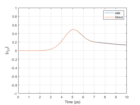
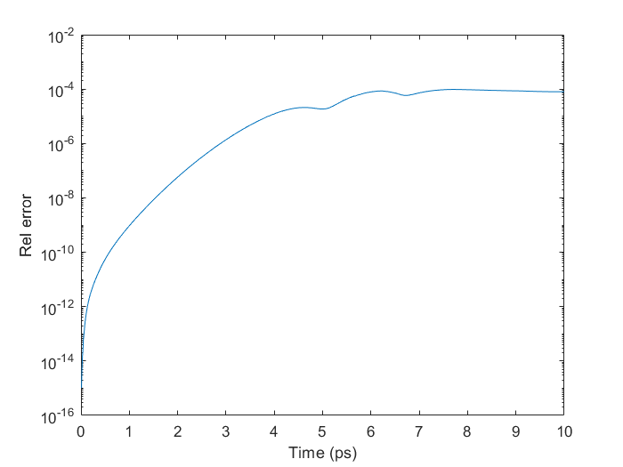
Figure 7: (Left) $|\tilde{\rho}_{01}|$ for a system of 128 quantum dots in a cube of length $\lambda/10$ (chosen to promote observable coupling effects through very close quantum dots), computed using the direct algorithm and AIM. (Right) Relative error of AIM algorithm against the direct algorithm for this simulation.

Figure 8: FFT runtime (excluding setup time) using a third-order expansion. (Top) 1024 timesteps with $\Delta s=\lambda/400$ and prescribed polarizations in the fixed frame. (Bottom) 1000 timesteps with $\Delta s=\lambda/10$ and Liouville-dynamics polarization in the rotating frame. Both cases have a quasi-quadratic scaling in the direct calculation, whereas the FFT-accelerated calculation performs slightly worse than linear.

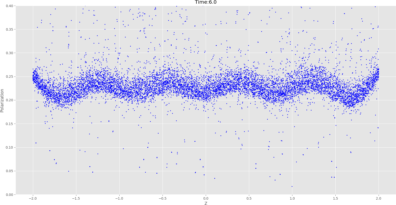
Figure 9: $\hat{\mathbf{z}}$-distribution of polarization $|\tilde{\rho}_{01}|$ for a $10\,000$-dot cylindrical simulation, replicating the parameters in [1]. The AIM calculation recovers the oscillatory long-range pattern that we obtained using a direct calculation [1].

5.4 Large scale physical simulations

The largest system simulated in [1] without TD-AIM consists of $10\,000$ quantum dots randomly distributed in a cylinder of radius $0.2\text{\,}\mathrm{\SIUnitSymbolMicro m}$ and length $4\text{\,}\mathrm{\SIUnitSymbolMicro m}$. Figure 9 shows an equivalent simulation with TD-AIM that reproduces features arising from quantum dot interactions; we conduct a very similar experiment here. The figure shows the polarization of each quantum dot in the cylinder as a function of their $\mathbf{z}$-coordinate (the axis of the cylinder), under the effect of a resonant $\pi$ pulse. Each of the quantum dots has an identical (fixed) dipole moment (see Ref.[1] for the details of the simulation parameters). Note how the secondary radiation produces random shifts in the polarization due to short-range effects in the local neighborhood of each quantum dot. In addition, the simulation shows an oscillation of the polarization due to long-range collective effects. This oscillation reflects the role of boundary conditions in the confinement of the macroscopic electric field in the system.

The algorithm introduced in this paper facilitates simulations of much larger systems. In figs. 10 and 11 we examine the response of a system of $100\,000$ quantum dots—randomly distributed throughout a cuboid—to an applied laser pulse traveling along $\hat{\mathbf{z}}$. The transition dipole moment of each quantum dot has a fixed magnitude but random orientation. Tables 1 and 2 list simulation parameters.

Quantity	Symbol	Value
Simulation timestep	$\Delta t$	$0.02$ ps
AIM spacing	$\Delta s$	$0.040\lambda=33.06$ nm
Transverse domain length	-	$16\>\Delta s=529$ nm
Longitudinal domain length	-	$1500\>\Delta s=49.59\>\mu$m

Table 2: AIM parameters for the simulation of Section 5.4

Fig 10 displays a color map of $\absolutevalue{\tilde{\rho}_{01}}$ as an indicator of the polarization $|\tilde{\textbf{P}}|$ of each quantum dot at different timesteps after the pulse peak. The figure shows only quantum dots located in a central segment of about $4\text{\,}\mathrm{\SIUnitSymbolMicro m}$ of the entire cuboid. The random orientation of the dipole moments creates a variation in the amplitude of the polarization with quantum dots whose dipole moments (anti-)align with the laser field having greatest amplitude. In addition, despite each quantum dot resonantly coupling to the pulse, inhomogeneity arises due to the inter-dot coupling. These simulation can resolve inhomogeneities at the microscopic level, taking into account the orientation of the transition dipole moment of each quantum dot, as well as the effect of local secondary fields.

To visualize long-range effects, fig. 11 shows $|\tilde{\rho}_{01}|$ as a function of the $\mathbf{z}$ coordinate of each quantum dot, corresponding to the color plots of fig. 10. Here we show the entire cuboid having sides of $20\text{\,}\mathrm{\SIUnitSymbolMicro m}$. In contrast to the results of fig. 9, we do not observe the oscillatory behavior due to confinement since the length of the system far exceeds the radiation wavelength. Moreover, we observe a dispersion of the polarization due to the random orientation of the transition dipoles. Since the strength of the coupling scales with $\mathbf{E}\cdot\mathbf{d}=\cos(\theta)$, the distribution peaks at the value of $|\tilde{\rho}_{01}|$ when $\theta=0$ or $\theta=\pi$, with a tail corresponding to all the intermediate values. Only a few quantum dots, for which the secondary fields constructively interfere, have a polarization larger than the peak value. Finally, note how the value of the peak polarization slightly increases from left to right due to pulse propagation.

Furthermore, we calculate the inverse participation ratio (IPR) of the dot polarization:

$$\text{IPR}(t)=\frac{\sum_{l}|\tilde{\rho}_{01}(t)|^{4}}{(\sum_{l}|\tilde{\rho}_{01}(t)|^{2})^{2}}$$ (2at)

with results shown in fig. 12. This quantity ranges from $1/N$ to $1$, and collectively measures the spatial localization of the polarization, with $1/N$ corresponding to a completely delocalized spatial distribution, and $1$ to the case of the polarization completely localised on as single site. For comparison, we also include an IPR plot for the case of uniform (pulse-aligned) dipoles. In the uniform case, all quantum dots participate equally until the onset of the pulse peak, whereupon inter-dot coupling leads certain quantum dots to retain their polarization longer than neighbors. This contrasts the non-uniform case, which exhibits localization of polarization to quantum dots that align with the laser pulse.

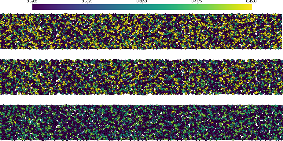
Figure 10: Coloration of $\absolutevalue{\tilde{\rho}_{01}}$ as an indicator of $|\tilde{\textbf{P}}|$ at $t_{1}=$2.0\text{\,}\mathrm{ps}$$ (top), $t_{2}=$3.0\text{\,}\mathrm{ps}$$ (middle), $t_{3}=$4.0\text{\,}\mathrm{ps}$$ (bottom) relative to the peak of a $1\text{\,}\mathrm{ps}$-wide pulse, for a system of $100\,000$ quantum dots.

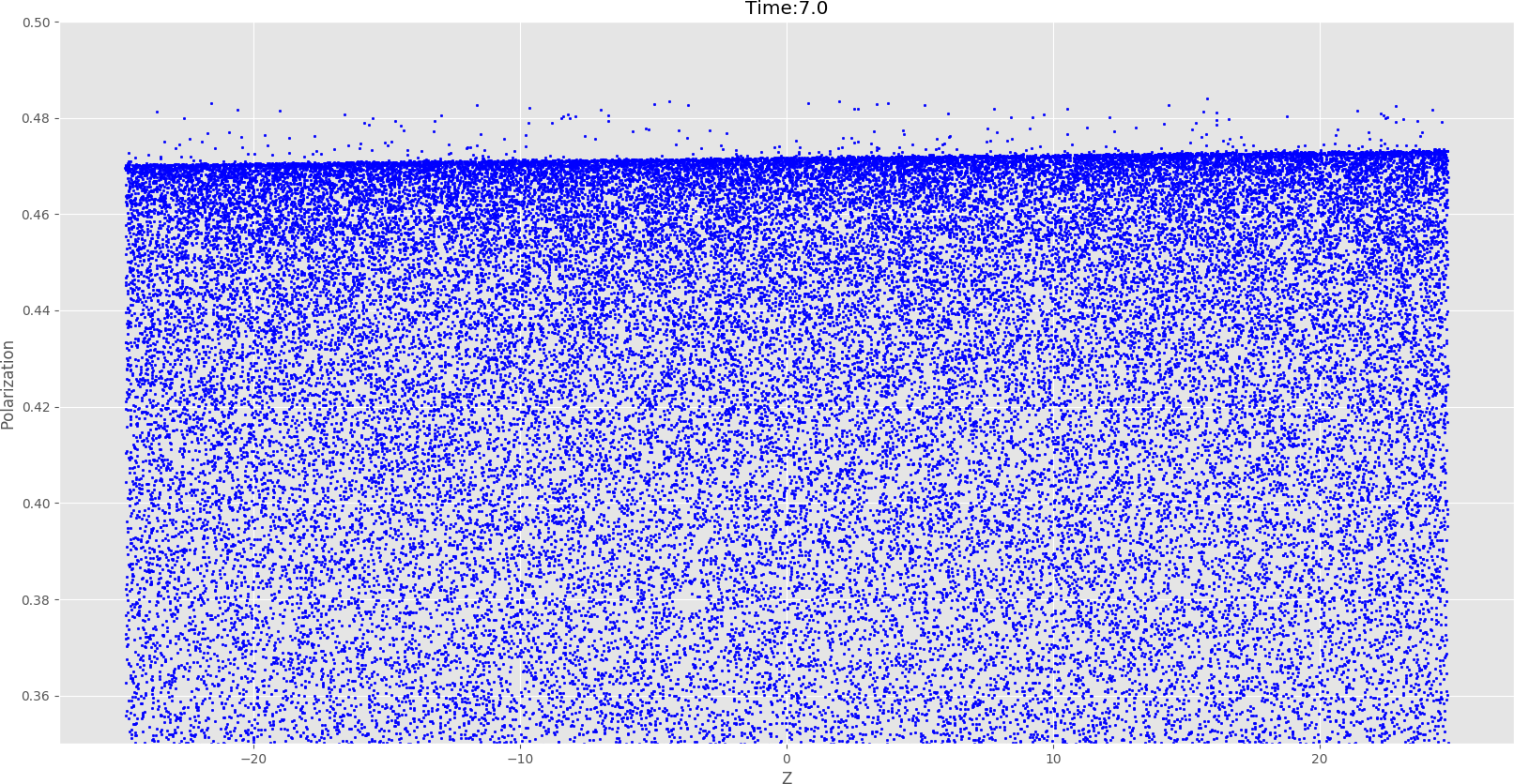
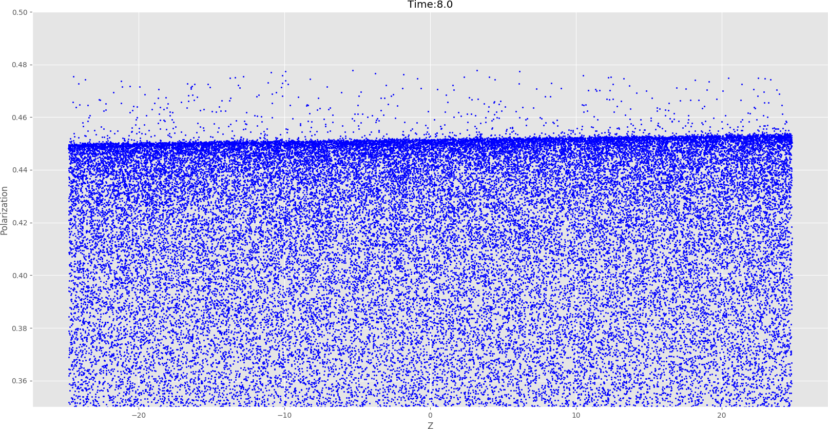
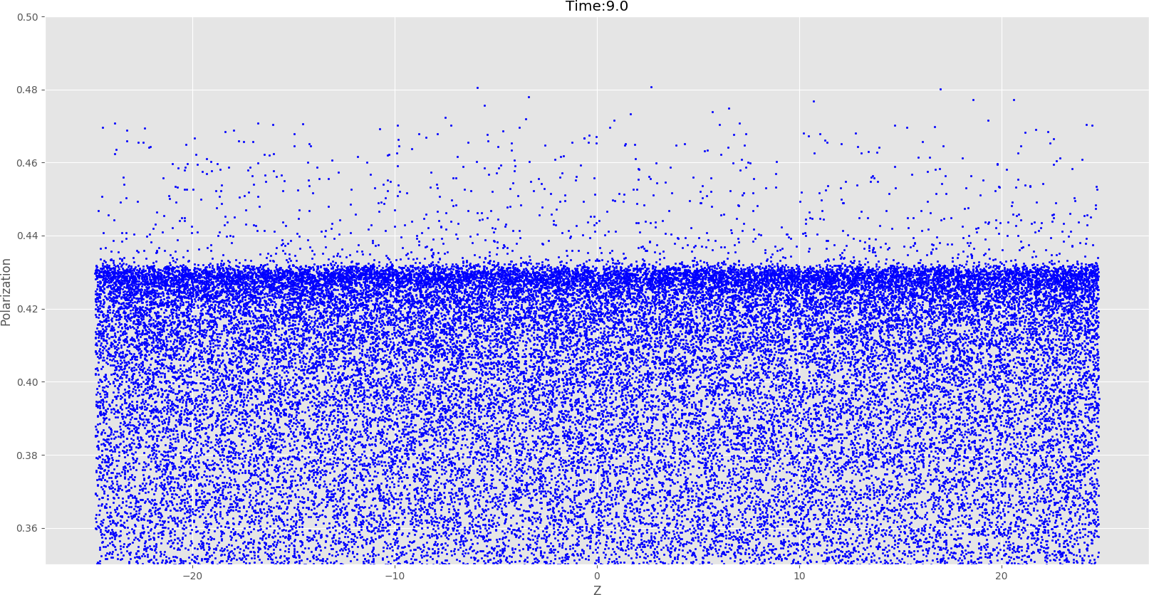
Figure 11: Scatterplots of $|\tilde{\rho}_{01}|$ corresponding to the color plots of fig. 10. There exists a single preferred polarization, represented by the linear region of greatest density, arising from quantum dots whose transition dipole moments (anti-)align with the laser field. Radiative coupling produces polarizations that exceeding this value.

Figure 12: Inverse Participation Ratio (IPR) for the system of fig. 10 (red) and a similar system of $100\,000$ quantum dots with uniform dipole orientations (blue).

6 Conclusions

Here we have presented novel variations to TD-AIM that enables analysis of large ensembles of quantum dots. We discuss Numerous features of the approach, including accuracy, convergence, and complexity. The latter for prescribed and fixed polarization, as well as when the polarization evolves. We validate the approach against “direct” simulations that use no acceleration techniques. Finally, we use the approach simulate a system with $100\,000$ dots. We observe identical results identical to direct solutions, thus these techniques can reliably simulate much larger systems. The next phase of our research focuses on additional functionality in both the physics as well as the computational infrastructure.

References

References

- [1] C. Glosser, B. Shanker, C. Piermarocchi, Collective rabi dynamics of electromagnetically coupled quantum-dot ensembles, Physical Review A 96 (3) (2017) 033816.
-
[2]
T. H. Stievater, X. Li, D. G. Steel, D. Gammon, D. S. Katzer, D. Park,
C. Piermarocchi, L. J. Sham,
Rabi
oscillations of excitons in single quantum dots, Phys. Rev. Lett. 87 (2001)
133603.
doi:10.1103/PhysRevLett.87.133603.
URL http://link.aps.org/doi/10.1103/PhysRevLett.87.133603 -
[3]
H. Kamada, H. Gotoh, J. Temmyo, T. Takagahara, H. Ando,
Exciton rabi
oscillation in a single quantum dot, Phys. Rev. Lett. 87 (2001) 246401.
doi:10.1103/PhysRevLett.87.246401.
URL https://link.aps.org/doi/10.1103/PhysRevLett.87.246401 -
[4]
H. Htoon, T. Takagahara, D. Kulik, O. Baklenov, A. L. Holmes, C. K. Shih,
Interplay of
rabi oscillations and quantum interference in semiconductor quantum dots,
Phys. Rev. Lett. 88 (2002) 087401.
doi:10.1103/PhysRevLett.88.087401.
URL https://link.aps.org/doi/10.1103/PhysRevLett.88.087401 -
[5]
G. Y. Slepyan, S. A. Maksimenko, A. Hoffmann, D. Bimberg,
Quantum optics of a
quantum dot: Local-field effects, Phys. Rev. A 66 (2002) 063804.
doi:10.1103/PhysRevA.66.063804.
URL http://link.aps.org/doi/10.1103/PhysRevA.66.063804 -
[6]
G. Y. Slepyan, A. Magyarov, S. A. Maksimenko, A. Hoffmann, D. Bimberg,
Rabi oscillations
in a semiconductor quantum dot: Influence of local fields, Phys. Rev. B 70
(2004) 045320.
doi:10.1103/PhysRevB.70.045320.
URL http://link.aps.org/doi/10.1103/PhysRevB.70.045320 -
[7]
K. Asakura, Y. Mitsumori, H. Kosaka, K. Edamatsu, K. Akahane, N. Yamamoto,
M. Sasaki, N. Ohtani,
Excitonic rabi
oscillations in self-assembled quantum dots in the presence of a local field
effect, Phys. Rev. B 87 (2013) 241301.
doi:10.1103/PhysRevB.87.241301.
URL https://link.aps.org/doi/10.1103/PhysRevB.87.241301 -
[8]
G. Rainò, M. A. Becker, M. I. Bodnarchuk, R. F. Mahrt, M. V. Kovalenko,
T. Stöferle,
Superfluorescence from lead
halide perovskite quantum dot superlattices, Nature 563 (7733) (2018)
671–675.
doi:10.1038/s41586-018-0683-0.
URL https://doi.org/10.1038/s41586-018-0683-0 -
[9]
M. Gross, S. Haroche,
Superradiance:
An essay on the theory of collective spontaneous emission, Physics Reports
93 (5) (1982) 301 – 396.
doi:http://dx.doi.org/10.1016/0370-1573(82)90102-8.
URL http://www.sciencedirect.com/science/article/pii/0370157382901028 - [10] S. L. McCall, E. L. Hahn, Self-induced transparency, Phys. Rev. 183 (1969) 457–485. doi:10.1103/PhysRev.183.457.
-
[11]
N. E. Rehler, J. H. Eberly,
Superradiance, Phys.
Rev. A 3 (1971) 1735–1751.
doi:10.1103/PhysRevA.3.1735.
URL http://link.aps.org/doi/10.1103/PhysRevA.3.1735 -
[12]
N. Bachelard, R. Carminati, P. Sebbah, C. Vanneste,
Linear and
nonlinear rabi oscillations of a two-level system resonantly coupled to an
anderson-localized mode, Phys. Rev. A 91 (2015) 043810.
doi:10.1103/PhysRevA.91.043810.
URL http://link.aps.org/doi/10.1103/PhysRevA.91.043810 - [13] A. Fratalocchi, C. Conti, G. Ruocco, Mode competitions and dynamical frequency pulling in Mie nanolasers: 3d ab-initio Maxwell-Bloch computations, Optics express 16 (12) (2008) 8342–8349.
-
[14]
C. Vanneste, P. Sebbah,
Selective
excitation of localized modes in active random media, Phys. Rev. Lett. 87
(2001) 183903.
doi:10.1103/PhysRevLett.87.183903.
URL http://link.aps.org/doi/10.1103/PhysRevLett.87.183903 - [15] A. Baczewski, Integral equation and discontinuous galerkin methods for the analysis of light-matter interaction, Ph.D. thesis, Michigan State University (2013).
- [16] D. Stynyk, Mathematical modeling of quantum dots with generalized envelope functions approximations and coupled partial differential equations, Master’s thesis, Wilfrid Laurier University (2009).
- [17] V. V. Temnov, U. Woggon, Photon statistics in the cooperative spontaneous emission, Optics express 17 (7) (2009) 5774–5782.
- [18] J. M. Jin, The Finite Element Method in Electromagnetics, Wiley, New York, 2002.
- [19] B. Shanker, A. A. Ergin, M. Lu, E. Michielssen, Fast analysis of transient electromagnetic scattering phenomena using the multilevel plane wave time domain algorithm, IEEE Transactions on Antennas and Propagation 51 (3) (2003) 628–641.
- [20] A. E. Yilmaz, J.-M. Jin, E. Michielssen, Time domain adaptive integral method for surface integral equations, IEEE Transactions on Antennas and Propagation 52 (10) (2004) 2692–2708. doi:10.1109/TAP.2004.834399.
- [21] G. Kobidze, J. Gao, B. Shanker, E. Michielssen, A fast time domain integral equation based scheme for analyzing scattering from dispersive objects, Antennas and Propagation, IEEE Transactions on 53 (3) (2005) 1215–1226. doi:10.1109/TAP.2004.841295.
- [22] E. Bleszynski, M. Bleszynski, T. Jaroszewicz, AIM: Adaptive integral method for solving large-scale electromagnetic scattering and radiation problems, Radio Science 31 (5) (1996) 1225–1251. doi:10.1029/96RS02504.
- [23] D. C. Rapaport, The Art of Molecular Dynamics Simulation, Cambridge University Press, 2004.
-
[24]
L. Landau, E. Lifshitz,
The Classical Theory of
Fields, Vol. 2 of Course of Theoretical Physics, Elsevier Science, 2013.
URL https://books.google.com/books?id=HudbAwAAQBAJ - [25] C. Cohen-Tannoudji, J. Dupont-Roc, G. Grynberg, Photons and atoms: introduction to quantum electrodynamics, Wiley Online Library, 1989.
-
[26]
L. Allen, J. Eberly,
Optical Resonance and
Two-level Atoms, Dover books on physics and chemistry, Dover, 1975.
URL https://books.google.com/books?id=1q0ae-XNmWwC - [27] A. J. Pray, N. V. Nair, B. Shanker, Stability properties of the time domain electric field integral equation using a separable approximation for the convolution with the retarded potential, IEEE Transactions on Antennas and Propagation 60 (8) (2012) 3772–3781. doi:10.1109/TAP.2012.2201101.
- [28] B. Shanker, A. A. Ergin, K. Aygun, E. Michielssen, Analysis of transient electromagnetic scattering from closed surfaces using a combined field integral equation, IEEE Transactions on Antennas and Propagation 48 (7) (2000) 1064–1074. doi:10.1109/8.876325.