Density estimation on an unknown submanifold

Abstract

We investigate density estimation from a $n$-sample in the Euclidean space $\mathbb{R}^{D}$, when the data are supported by an unknown submanifold $M$ of possibly unknown dimension $d<D$, under a reach condition. We investigate several nonparametric kernel methods, with data-driven bandwidths that incorporate some learning of the geometry via a local dimension estimator. When $f$ has Hölder smoothness $\beta$ and $M$ has regularity $\alpha$, our estimator achieves the rate $n^{-\alpha\wedge\beta/(2\alpha\wedge\beta+d)}$ for a pointwise loss. The rate does not depend on the ambient dimension $D$ and we establish that our procedure is asymptotically minimax for $\alpha\geq\beta$. Following Lepski’s principle, a bandwidth selection rule is shown to achieve smoothness adaptation. We also investigate the case $\alpha\leq\beta$: by estimating in some sense the underlying geometry of $M$, we establish in dimension $d=1$ that the minimax rate is $n^{-\beta/(2\beta+1)}$ proving in particular that it does not depend on the regularity of $M$. Finally, a numerical implementation is conducted on some case studies in order to confirm the practical feasibility of our estimators.

Mathematics Subject Classification (2010): 62C20, 62G05, 62G07.

Keywords: Point clouds, manifold reconstruction, nonparametric estimation, adaptive density estimation, kernel methods, Lepski’s method.

1 Introduction

1.1 Motivation

Suppose we observe an $n$-sample $(X_{1},\ldots,X_{n})$ of size $n$ distributed on an Euclidean space $\mathbb{R}^{D}$ according to some density function $f$. We wish to recover $f$ at some point arbitrary point $x\in\mathbb{R}^{D}$ nonparametrically. If the smoothness of $f$ at $x$ measured in a strong sense is of order $\beta$ – for instance by a Hölder condition or with a prescribed number of derivatives – then the optimal (minimax) rate for recovering $f(x)$ is of order $n^{-\beta/(2\beta+D)}$ and is achieved by kernel or projection methods, see e.g. the classical textbooks Silverman (1986); Devroye and Györfi (1985) or (Tsybakov, 2008, Sec. 1.2-1.3). Extension to data-driven bandwidths (Bowman, 1984; Chiu, 1991) offers the possibly to adapt to unknown smoothness, see (Goldenshluger and Lepski, 2008, 2011, 2014) for a modern mathematical formulation. More generally, recommended reference on adaptive estimation is the textbook by Giné and Nickl (2016). In many situations however, the dimension $D$ of the ambient space is large, hitherto disqualifying such methods for pratical applications. Opposite to the curse of dimensionality, a broad guiding principle in practice is that the observations $(X_{1},\ldots,X_{n})$ actually live on smaller dimensional structures and that the effective dimension of the problem is smaller if one can take advantage of the geometry of the data (Fefferman et al., 2016). This classical paradigm probably goes back to a conjecture of (Stone, 1982) that paved the way to the study of the celebrated single-index model in nonparametric regression, where a structural assumption is put in the form $f(x)=g(\langle\vartheta,x\rangle)$, where $\langle\cdot,\cdot\rangle$ is the scalar product on $\mathbb{R}^{D}$, for some unknown univariate function $g:\mathbb{R}\rightarrow\mathbb{R}$ and direction $\vartheta\in\mathbb{R}^{D}$. Under appropriate assumptions, the minimax rate of convergence for recovering $f(x)$ with smoothness $\beta$ drops to $n^{-\beta/(2\beta+1)}$ and does not depend on the ambient dimension $D$, see e.g. (Gaïffas and Lecué, 2007; Lepski and Serdyukova, 2014) and the references therein. Also, in the search for significant variables, one postulates that $f$ only depends on $d<D$ coordinates, leading to the structural assumption $f(x_{1},\ldots,x_{D})=F(x_{i_{1}},\ldots x_{i_{d}})$ for some unknown function $F:\mathbb{R}^{d}\rightarrow\mathbb{R}$ and $\{i_{1},\ldots,i_{d}\}\subset\{1,\ldots,D\}$. In an analogous setting, the minimax rate of convergence becomes $n^{-\beta/(2\beta+d)}$ and this is also of a smaller order of magnitude than $n^{-\beta/(2\beta+D)}$, see (Hoffmann and Lepski, 2002) in the white noise model.

The next logical step is to assume that the data $(X_{1},\ldots,X_{n})$ live on a $d$-dimensional submanifold $M$ of the ambient space $\mathbb{R}^{D}$. When the manifold is known prior to the experiment, nonparametric density estimation dates back to (Devroye and Györfi, 1985) when $M$ is the circle, and on a homogeneous Riemannian manifold by (Hendriks, 1990), see also Pelletier (2005). Several results are known for specific geometric structures like the sphere or the torus involved in many applied situations: inverse problems for cosmological data (Kim and Koo, 2002; Kim et al., 2009; Kerkyacharian et al., 2011), in geology (Hall et al., 1987) or flow calculation in fluid mechanics (Eugeciouglu and Srinivasan, 2000). For genuine compact homogeneous Riemannian manifolds, a general setting for smoothness adaptive density estimation and inference has recently been considered by Kerkyacharian et al. (2012), or even in more abstract metric spaces in Cleanthous et al. (2018). See also Baldi et al. (2009); Castillo et al. (2014) and the references therein. A common strategy adapts conventional nonparametric tools like projection or kernel methods to the underlying geometry, via the spectral analysis of the Beltrami-Laplace operator on $M$. Under appropriate assumptions, this leads to exact or approximate eigenbases (spherical harmonics for the sphere, needlets and so on) or properly modified kernel methods, according to the Riemannian metric on $M$.

If the submanifold $M$ itself is unknown, getting closer in spirit to a dimension reduction approach, the situation becomes drastically different: $M$ hence its geometry is unknown, and considered as a nuisance parameter. In order to recover the density $f$ at a given point $x\in\mathbb{R}^{D}$ of the ambient space, one has to understand the minimal geometry of $M$ that must be learned from the data and how this geometry affects the optimal reconstruction of $f$. This is the topic of the paper.

We consider in the paper a seemingly unusual framework where the support of a distribution is unknown while the aim is to recover the density at a point $x\in\mathbb{R}^{D}$ which is known to be on the support. As mentioned above, this actually covers at least two situations:

• The data are high-dimensional and it is reasonable to believe that they actually lie on a smaller dimensional subset of the ambient space $\mathbb{R}^{D}$, which can be assumed to be a submanifold. In that case, $x$ can be seen as an observation $X_{0}$ from our dataset, and the analysis can be (implicitly) performed conditional on $X_{0}$;

• The data naturally lie on a submanifold, like a spheroid for geological application, or a cell membrane in microbiology (see for instance Klein et al. (2014) who describe a technique that yields such a point cloud). In this case, $x$ can be seen as an observation $X_{0}$ like above, but there is also the situation where the statistician can know whether or not a given point $x$ is within the support (for instance a point on a cell membrane, or a geographical location on the Earth surface) without knowing the geometric feature of the latter and without needing to estimate them.

1.2 Main results

We construct a class of compact smooth submanifolds of dimension $d$ of the Euclidean space $\mathbb{R}^{D}$, without boundaries, that constitute generic models for the unknown support of the target density $f$ that we wish to reconstruct. We further need a reach condition, a somehow unavoidable notion in manifold reconstruction that goes back to Federer (1959): it is a geometric invariant that quantifies both local curvature conditions and how tightly the submanifold folds on itself. It is related to the scale at which the sampling rate $n$ can effectively recover the geometry of the submanifold, see Section 2.3 below. We consider regular manifolds $M$ with reach bounded below that satisfy the following property: $M$ admits a local parametrization at every point $x\in M$ by its tangent space $T_{x}M$, and this parametrization is sufficiently regular. A natural candidate is given by the exponential map $\exp_{x}:T_{x}M\rightarrow M\subset\mathbb{R}^{D}$. More specifically, for some regularity parameter $\alpha\geq 0$, we require a certain uniform bound for the $\alpha+1$-fold differential of the exponential map to hold, quantifying in some sense the regularity of the parametrization in a minimax spirit. Our approach is close to that of Aamari and Levrard (2019, Def. 1) that consider arbitrary parametrizations among those close to the inverse of the projection onto tangent spaces. Given a density function $f:M\rightarrow[0,\infty)$ with respect to the volume measure on $M$, we have a natural extension of smoothness spaces on $M$ by requiring that $f\circ\exp_{x}:T_{x}M\rightarrow\mathbb{R}$ is a smooth map in any reasonable sense, see for instance Triebel (1987) for the characterisation of function spaces on a Riemannian manifold.

Our main result is that in order to reconstruct $f(x)$ efficiently at a point $x\in\mathbb{R}^{D}$ when $f$ has smoothness $\beta$ and lives on an unknown submanifold of smoothness $\alpha$ and unknown dimension $d<D$, it is sufficient to consider estimators of the form

$$\widehat{f}_{h}(x)=\frac{1}{nh^{\widehat{d}(x)}}\sum_{i=1}^{n}K\left(\frac{x-X_{i}}{h}\right),~{}~{}x\in\mathbb{R}^{D},$$ (1)

where $K:\mathbb{R}^{D}\rightarrow\mathbb{R}$ is a certain kernel and $\widehat{d}(x)=\widehat{d}(x,X_{1},\ldots,X_{n})$ is an estimator of the local dimension of the support of $f$ in the vicinity of $x$ based on a scaling estimator as introduced in Farahmand et al. (2007). We prove in Theorem 3.1 that following a classical bias-variance trade-off for the bandwidth $h$, the rate $n^{-\alpha\wedge\beta/(2\alpha\wedge\beta+d)}$ is achievable for pointwise and global loss when the dimension of $M$ is $d$, irrespectively of the ambient dimension $D$. In particular, it is noteworthy that in terms of manifold learning, only the dimension of $M$ needs to be estimated. When $\alpha\geq\beta$, we also have a lower bound (Theorem 3.2) showing that our result is minimax optimal. Moreover, by implementing Lepski’s principle (Lepskii, 1992), we are able to construct a data driven bandwidth $\widehat{h}=\widehat{h}(x,X_{1}\ldots,X_{n})$ that achieves in Theorem 3.4 the rate $n^{-\alpha\wedge\beta/(2\alpha\wedge\beta+d)}$ up to a logarithmic term — unavoidable in the case of pointwise loss due to the Lepski-Low phenomenon (Lepskiĭ, 1990; Low, 1992). When the dimension $d$ is known, the estimator (1) has already been investigated in squared-error norm in Ozakin and Gray (2009) for a fixed manifold $M$ and smoothness $\beta=2$.

A remaining issue at this stage is to understand how the regularity of $M$ can affect the minimax rates of convergence for smooth functions, i.e. when $\alpha\leq\beta$. We only have a partial answer to that question, when we restrict our attention to the one-dimensional case $d=1$. When $M$ is known, Pelletier (2005) studied estimators of the form

$$\frac{1}{nh^{d}}\sum_{i=1}^{n}\frac{1}{\vartheta_{x}(X_{i})}K\left(\frac{d_{M}(x,X_{i})}{h}\right),$$ (2)

where $K:\mathbb{R}\rightarrow\mathbb{R}$ is a radial kernel, $d_{M}$ is the intrinsic Riemannian distance on $M$ and the correction term $\vartheta_{x}(X_{i})$ is the volume density function on $M$ (Besse, 1978, p. 154) that accounts for the value of the density of the volume measure at $X_{i}$ in normal coordinates around $x$, taking into account how the submanifold curves around $X_{i}$. By establishing in Lemma 3.9 that $\vartheta_{x}$ is constant (and identically equal to one) when $d=1$, we have another estimator by simply learning the geometry of $M$ via its intrinsic distance $d_{M}$ in (2). This can be done by efficiently estimating $d_{M}$ in dimension $d=1$ thanks to the Isomap method as coined by Tenenbaum et al. (2000). Therefore, in the special case when the dimension $d$ of $M$ is known and equal to $1$, we are able to construct an estimator that achieves in Theorem 3.3 the rate $n^{-\beta/(2\beta+1)}$, therefore establishing that in dimension $d=1$ at least, the regularity of the manifold $M$ does not affect the minimax rate for estimating $f$ even when $M$ is unknown. However, the volume density function $\vartheta_{x}$ is not constant as soon as $d\geq 2$ and obtaining a global picture in higher dimensions remains an open and presumably challenging problem.

1.3 Organisation of the paper

In Section 2, we provide with all the necessary material and notation from classical geometry for the unfamiliar reader. Section 2.1 together with the construction of smoothness spaces – here Hölder spaces on a submanifold in Section 2.2. We elaborate in particular on the reach of a subset of the Euclidean space in Section 2.3 and construct a statistical model for sampling $n$ data from a density $f$ with regularity $\beta$ living on an unknown submanifold $M$ of unknown dimension $d$ and smoothness $\alpha$ in an ambient space of dimension $D$ in Section 2.4. In this setting, we establish in Section 2.5 that a reach condition, i.e. assuming that the reach of $M$ is bounded below, is necessary in order to reconstruct $d$. This is stated precisely in Theorem 2.6.

We give our main results in Section 3.1 and more specifically in Section 3.1. When the dimension $d$ and the smoothness parameters $\alpha$ of the unknown manifold $M$ and the smoothness $\beta$ of $f$ are known, Theorem 3.1 states the existence of an estimator that achieves the rate $n^{-\alpha\wedge\beta/(2\alpha\wedge\beta+d)}$ in expected pointwise loss, and Theorem 3.2 establishes that a minimax lower bound is $n^{-\beta/(2\beta+d)}$. Theorem 3.3 shows the existence of estimators in dimension $d=1$ that achieve the rate $n^{-\beta/(2\beta+1)}$, which is therefore minimax in that case. Theorem 3.4 states the existence of smoothness and dimension adaptive estimators, when $\alpha,\beta$ and $d$ are unknown. Section 3.2 elaborates on special kernels upon which the estimators that achieve the aforementioned results are constructed, and their properties with respect to bias and variance analysis. The underlying geometry of $M$ makes the usual orthogonality to non-constant polynomials of a certain degree (the order of the kernel) irrelevant, and a specific construction must be undertaken. Section 3.3 focuses on the case of one-dimensional submanifolds $M$ when $d=1$, where we explicitly construct a kernel estimator that achieves the minimax rate of convergence, revisiting the estimator (2) of Pelletier (2005) and relying on the Isomap algorithm. In Section 3.4, we implement Lepski’s algorithm on the bandwidth of our kernel estimators, following Lepski et al. (1997); this achieves smoothness adaptation w.r.t. $\alpha\wedge\beta$. Finally, in Section 3.5, we build an estimator of the dimension $d$ of $M$, following ideas of Farahmand et al. (2007) and that enables us to obtain simultaneous adaptation w.r.t. $\alpha\wedge\beta$ and $d$ by plug-in.

Finally, numerical examples are developed in Section 4: we elaborate on examples of non-isometric embeddings of the circle and the torus in dimension 1 and 2 and explore in particular rates of convergence on Monte-Carlo simulations, illustrating how effective Lepski’s method can be in that context. The proof are delayed until Appendix A.

2 Manifold-supported probability distributions

2.1 Some material from classical geometry

We recall some basic notions of geometry of submanifolds of the Euclidean space $\mathbb{R}^{D}$ for the unfamiliar reader. We borrow material from the classical textbooks Gallot et al. (2004) and Lee (2006). We endow $\mathbb{R}^{D}$ with its usual Euclidean product and norm, respectively denoted by $\langle\cdot,\cdot\rangle$ and $\|\cdot\|$. We denote by $B(x,r)$ the open ball of $\mathbb{R}^{D}$ of center $x$ and radius $r$, and, for any supspace $H\subset\mathbb{R}^{D}$, $B_{H}(x,r)$ the open ball of in $H$ for the induced norm (namely $B_{H}(x,r)=H\cap B(x,r)$).

Classicaly, the smoothness of a submanifold is defined through the regularity of its parametrizations. Because we will need to compare quantitatively the smoothness of manifold within a large class, we will have to pick one canonical way of parametrizing them. For this reason, we consider the exponential map; for any smooth submanifold $M\subset\mathbb{R}^{D}$ and any $x\in M$, it defines a smooth parametrization

$$\exp_{x}:B_{T_{x}M}(0,\varepsilon)\to M$$

of $M$ around $x$, provided that $\varepsilon$ is chosen small enough (Gallot et al., 2004, Cor 2.89 p.86). The supremum of all such $\varepsilon$ is called the injectivity radius at $x$ and is denoted $\operatorname{inj}_{M}(x)$. When $M$ is a closed subset of $\mathbb{R}^{D}$, the exponential maps are well defined on the whole tangent spaces. This is (one side of) the Hopf-Rinow theorem (Lee, 2006, Thm 6.13 p.108).

Given a submanifold $M$ of dimension $d$, we will define the volume measure of $M$, denoted by $\mu_{M}$, as the restriction of the $d$-dimensionnal Hausdorff measure $\mathcal{H}^{d}$ to $M$, see Federer (1969, Sec 2.10.2 p.171) for a definition. It can be shown (Evans and Gariepy, 1992, Ex D p.102) that this definition coincides with the usual one of volume measure of a Riemaniann manifold, namely, if $\psi:M\rightarrow\mathbb{R}$ is a continuous fonction with support in $\exp_{x}(B_{T_{x}M}(0,\varepsilon))$ for $\varepsilon$ smaller than $\operatorname{inj}_{M}(x)$, we have

$$\mu_{M}(\psi)=\int_{B_{T_{x}M}(0,\varepsilon)}\psi\circ\exp_{x}(v)\sqrt{\det g_{ij}^{x}(v)}dv,$$

with $g_{ij}^{x}(v)=\langle d\exp_{x}(v)[e_{i}],d\exp_{x}(v)[e_{j}]\rangle$ and where $(e_{1},\dots,e_{d})$ is an arbitrary orthonormal basis of $T_{x}M$. See Gallot et al. (2004, Sec 3.H.1 and Sec 3.H.2) for further details on the volume measure. The volume of $M$, denoted by $\operatorname{vol}M$, is simply $\mu_{M}(\mathbbm{1})$. It is finite in particular when $M$ is a compact submanifold of $\mathbb{R}^{D}$.

2.2 Hölder spaces on submanifolds of $\mathbb{R}^{D}$

Let $M$ be a smooth submanifold of $\mathbb{R}^{D}$. We say that a vector-valued function $f:M\to\mathbb{R}^{m}$ with $m\geq 1$ is $\gamma$-Hölder with $\gamma>0$ if for all $x\in M$, the map

$$f\circ\exp_{x}:B_{T_{x}M}(0,\rho)\to\mathbb{R}^{m}~{}~{}~{}~{}\text{where}~{}~{}\rho=\operatorname{inj}_{M}(x)$$

is $\gamma$-Hölder in the usual sense, namely

• $f\circ\exp_{x}$ is $k=\lceil\gamma-1\rceil$-times differentiable;

• and verifies

  $$\forall v,w\in B_{T_{x}M}(0,\rho),~{}~{}~{}~{}\|d^{k}(f\circ\exp_{x})(v)-d^{k}(f\circ\exp_{x})(w)\|_{\operatorname{op}}\leq R\|v-w\|^{\delta}$$

  with $\delta=\gamma-k>0$ and for some $R>0$.

We will denote by $\mathcal{H}^{\alpha}(M,\mathbb{R}^{m})$ the space of all such functions, and define for $f\in\mathcal{H}^{\alpha}(M,\mathbb{R}^{m})$ the Hölder coefficient

$$\|f\|_{\mathcal{H}^{\alpha}}=\sup_{x\in M}\sup_{\begin{subarray}{c}v,w\in B_{T_{x}M}(0,\rho)\\ \rho=\operatorname{inj}_{M}(x)\end{subarray}}\frac{\|d^{k}(f\circ\exp_{x})(v)-d^{k}(f\circ\exp_{x})(w)\|_{\operatorname{op}}}{\|v-w\|^{\delta}}.$$

Remark 2.1.

The characterization of the smoothness of a function $f:M\to\mathbb{R}^{m}$ through the exponential maps is a classical way to define functional spaces over Riemannian manifolds, see for instance Triebel (1987).

2.3 The reach of a subset

One of the main concern when dealing with observations sampled from a geometrically structured probability measure is to determine the suitable scale at which one should look at the data. Indeed, given finite-sized point cloud in $\mathbb{R}^{D}$, there are infinitely many submanifolds that interpolate the point cloud, see Figure 1 for an illustration. A popular notion of regularity for a subset of the Euclidean space is the reach, introduced by Federer (1959).

Figure 1: An arbitrary points cloud (Left) for $D=2$, and two smooth one-dimensional submanifolds passing through all its points (Middle, Right). A reach condition tends to discard the Right manifold as a likely candidate among all possible submanifolds the point cloud is sampled from.

Definition 2.1.

Let $K$ be a compact subset of $\mathbb{R}^{D}$. The reach $\tau_{K}$ of $K$ is the supremum of all $r\geq 0$ such that the orthogonal projection $\operatorname{pr}_{K}$ on $K$ is well-defined on the $r$-neighbourhood $K^{r}$ of $K$, namely

$$\tau_{K}=\sup\{r\geq 0~{}|~{}\forall x\in\mathbb{R}^{D},~{}d(x,K)\leq r\Rightarrow\exists!y\in K,~{}d(x,K)=\|x-y\|\}.$$

When $M$ is a compact submanifold of $\mathbb{R}^{D}$, the reach $\tau_{M}$ quantifies two geometric invariants: locally, it measures how curved the manifold is, and globally, it measures how close it is to intersect itself (the so-called bottleneck effect). See Figure 2 for an illustration of the phenomenon. A reach condition, meaning that the reach is bounded below, is necessary in order to obtain minimax inference results in manifold learning. These include: homology inference Niyogi et al. (2008); Balakrishnan et al. (2012), curvature (Aamari and Levrard, 2019) and reach estimation itself (Aamari et al., 2019) as well as manifold estimation Genovese et al. (2012); Aamari and Levrard (2019).

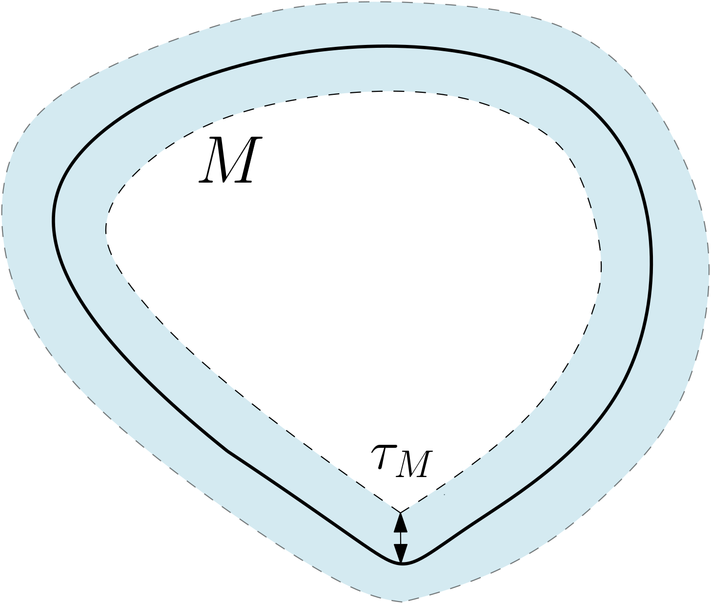
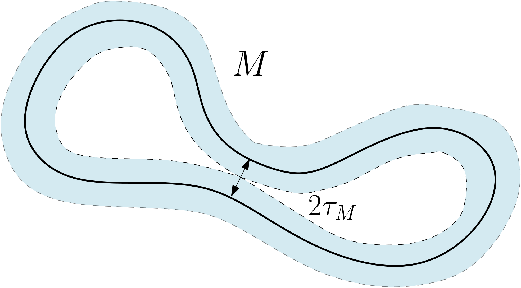
Figure 2: For the first manifold $M$ (Left), the value of the reach $\tau_{M}$ comes from its curvature. For the second one (Right), the reach is equal to $\tau_{M}$ because it is close to self intersecting (a bottleneck effect). The blue area represents the tubular neighbourhood over which the orthonormal projection on each manifold is well-defined.

2.4 A statistical model for sampling on a unknown manifold

In the following, we fix a point $x\in\mathbb{R}^{D}$ in the ambient space. See Section 1.1 for a discussion on such a setting. Our statistical model is characterized by two quantities: the regularity of its support and the regularity of the density defined on this support. The support belongs to a class of submanifolds $M$, for which we need to fix some kind of canonical parametrization. This is what Aamari and Levrard (2019) propose by asking the support $M$ to admit a local parametrization at all point $y\in M$ by $T_{y}M$, and that this parametrization is close to being the inverse of the projection over this tangent space. We follow this idea by imposing a constraint on the exponential map.

Definition 2.2.

Let $1\leq d<D$ be integers and $\tau>0$. We let $\mathcal{C}_{d}(\tau)$ define the set of submanifolds $M$ of $\mathbb{R}^{D}$ that contains $x$ and satisfying the following properties:

• (Dimension) $M$ is a smooth submanifold of dimension $d$ without boundaries;

• (Compactness) $M$ is compact;

• (Reach condition) We have $\tau_{M}\geq\tau$.

For $\alpha\geq 0$ and $L>0$, we define $\mathcal{C}_{d,\alpha}(\tau,L)$ as the set of $M\in\mathcal{C}_{d}(\tau)$ that fulfill the additional condition:

• The inclusion map $\iota_{M}:M\hookrightarrow\mathbb{R}^{D}$ is $(\alpha+1)$-Hölder with $\|\iota_{M}\|_{\mathcal{H}^{\alpha+1}}\leq L$.

Remark 2.2.

The definitions above endow our model with global constraints, even though most of them can be stated in a local fashion, with properties of the support holding in a neighborhood of our candidate point $x\in\mathbb{R}^{D}$. This meets two expectations:

• staying close to the existing manifold setting in statistics, like in Aamari and Levrard (2019);

• allowing for further developments, like estimation in global losses, such as $L^{p}$-norms, Wasserstein norms, or the sup-norm Wu and Wu (2020).

The reach condition $\tau_{M}\geq\tau>0$ in $(iii)$ is essential in estimating consistently a density at a point in our setting, as shown in Theorem 2.6 in Section 2.5. Furthermore, a reach constraint enables the use of a number of interesting geometric results.

Proposition 2.3.

Let $M$ be a compact smooth submanifold of $\mathbb{R}^{D}$ with $\tau_{M}\geq\tau$. Then the injectivity radius $\operatorname{inj}_{M}$ is everywhere greater than $\pi\tau$.

This result is a corollary of Alexander and Bishop (2006, Thm 1.3), as explained in Aamari and Levrard (2019, Lem A.1). Pick $M\in\mathcal{C}_{d}(\tau)$. For any $z\in M$, the map $v\mapsto\exp_{z}(v)-x$ is bounded on $B_{T_{z}M}(0,\pi\tau)$ by $\pi\tau$, since for any $v\in B_{T_{z}M}(0,\pi\tau)$, we have $\|\exp_{z}(v)-x\|\leq d_{M}(\exp_{z}(v),x)=\|v\|$, where $d_{M}$ is the intrinsic distance on $M$. This uniform bound along with the Hölder condition $(iv)$ allows one to obtain a uniform bound on the first derivatives of the exponential map

Lemma 2.4.

For $M\in\mathcal{C}_{d,\alpha}(\tau,L)$, any $z\in M$, and any $1\leq j\leq\lceil\alpha\rceil$, we have

$$\sup_{v\in B_{T_{z}M}(0,\pi\tau/2)}\|d^{j}\exp_{z}(v)\|_{\operatorname{op}}\leq L_{j},$$

with $L_{j}$ depending on $d$, $\tau$, $L$ and $\alpha$ only.

See Lemma A.6 in the appendix for further details on the proof. In the light of this result, the model of Definition 2.2 is thus quite close to the one proposed by Aamari and Levrard (2019). We are ready to define the class of density functions that we study, built upon submanifolds in the class $\mathcal{C}_{d}(\tau)$.

Definition 2.5.

Let $1\leq d\leq D-1$, $\alpha\geq 0$, $\beta\geq 0$, $\tau>0$, $L>0$, $R>0$ and $0\leq f_{\min}<f_{\max}$. We define $\Sigma^{d}_{\alpha,\beta}(\tau,L,f_{\min},f_{\max},R)$, or $\Sigma^{d}_{\alpha,\beta}$ for short, as the set of probability measures $P$ on $\mathbb{R}^{D}$ (endowed with its Borel $\sigma$-field) such that

• There exists $M_{P}\in\mathcal{C}_{d,\alpha}(\tau,L)$ such that $\operatorname{supp}P=M_{P}$;

• There exists a version of the Radon-Nikodym derivative $\frac{dP}{d\mu_{M_{P}}}$, denoted by $f_{P}$, that belongs to $\mathcal{H}^{\beta}(M_{P},\mathbb{R})$;

• This version satisfies $f_{\min}\leq f_{P}\leq f_{\max}$ and $\|f_{P}\|_{\mathcal{H}^{\beta}}\leq R$.

Some remarks: 1) By construction, the support of $P\in\Sigma^{d}_{\alpha,\beta}(\tau,L,f_{\min},f_{\max},R)$ all contains the candidate point $x$, see Definition 2.2. 2) Condition (i) discards the possibility that $f_{P}$ is zero on non-null subset of $M$; in particular $f_{P}$ is non zero around $x$ (but can be zero at $x$ nonetheless). This ensures that $x$ does not lie too far from the data. An alternate definition is to impose a condition like $P\ll\mu_{M}$. This leads to the same results in the next sections, but with a slight ambiguity in the choice of $M$. 3) The parameters in subscript or superscript $(d,\alpha,\beta)$ control the rate of convergence of the estimation, while the parameters $(\tau,L,f_{\min},f_{\max},R)$ control the pre-factor in the rates of convergence. For notational simplicity, we sometimes omit them when no confusion can be made.

2.5 Choice of a loss function and the reach assumption

For $P\in\Sigma^{d}_{\alpha,\beta}$ and a $n$-sample $(X_{1},\dots,X_{n})$ drawn from $P$, our goal is to recover the value of $f_{P}(x)$ thanks to an estimator $\widehat{f}(x)$ built on top of the data $(X_{1},\dots,X_{n})$. We measure the accuracy of estimation by the maximal expected risk or order $p$, for $p\geq 1$, defined by

$$\sup_{P\in\Sigma^{d}_{\alpha,\beta}}\mathbb{E}_{P^{\otimes n}}[|\widehat{f}(x)-f_{P}(x)|^{p}]^{1/p}$$

We look for an estimator with the smallest possible maximal risk as the number of observations $n$ goes to $\infty$. We first show that if we let $\tau=0$, i.e. if we do not impose a reach condition, then it is impossible to estimate $f(x)$ consistently as $n\to\infty$ for any estimator, thus establishing that the reach assumption $\tau>0$ unavoidable.

Theorem 2.6.

In the setting of Definition 2.5, if we let $\tau=0$, the following lower bound holds

$$\inf_{\widehat{f}(x)}\sup_{P\in\Sigma^{d}_{\alpha,\beta}}\mathbb{E}_{P^{\otimes n}}[|\widehat{f}(x)-f_{P}(x)|^{p}]^{1/p}\geq\frac{1}{2}(f_{\max}-f_{\min})>0,$$

where the infimum is taken over all estimators $\widehat{f}(x)$ of $f(x)$.

The proof is given in Appendix A.2. This result is in line with a reach condition $\tau>0$, a customary necessary condition in a minimax reconstruction in geometric inference, when the manifold is unknown, see (Niyogi et al., 2008; Genovese et al., 2012; Balakrishnan et al., 2012; Kim et al., 2016; Aamari and Levrard, 2019) and the references therein.

3 Density estimation at a fixed point

Recall that we fix the point $x\in\mathbb{R}^{D}$ where we wish to estimate $f$. Throughout the section, the symbols $\lesssim$ and $\gtrsim$ denote inequalities up to a constant that, unless specified otherwise, depend on the parameters $d,\alpha,\beta,\tau,L,f_{\min},f_{\max},R$ and $p$. The expression for $n$ large enough means for $n$ bigger than a constant that depends on the same parameters.

3.1 Main results

Let $D\geq 2$, $\tau>0$, $L>0$, $R>0$, $0\leq f_{\min}<f_{\max}$ and $p\geq 1$. Recall that we write $\Sigma^{d}_{\alpha,\beta}$ for short for $\Sigma^{d}_{\alpha,\beta}(\tau,L,f_{\min},f_{\max},R)$ as defined in Definition 2.5. The main results of this section are the following

Theorem 3.1 (Upper bound).

For any $1\leq d\leq D-1$, $\alpha\geq 0$ and $\beta\geq 0$, there exists an estimator $\widehat{f}(x)$ – explicitly constructed in Section 3.2 below – depending on $\alpha,\beta$ and $d$, such that, for $n$ large enough,

$$\sup_{P\in\Sigma^{d}_{\alpha,\beta}}\mathbb{E}_{P^{\otimes n}}[|\widehat{f}(x)-f_{P}(x)|^{p}]^{1/p}\lesssim n^{-\alpha\wedge\beta/(2\alpha\wedge\beta+d)}.$$

The estimator of Theorem 3.1 is a kernel density estimator that depends on $\alpha,\beta$ and $d$ through the choice of the kernel and its order (in a certain sense specified below), together with its bandwidth. Its analysis si given in Section 3.2. The estimator is indeed optimal in a minimax sense, as soon as $\alpha\geq\beta$

Theorem 3.2 (Lower bound).

Let $1\leq d\leq D-1$, $\alpha\geq 0$ and $\beta\geq 0$. If $L$ and $f_{\max}$ are large enough and if $f_{\min}$ is small enough (depending on $\tau$), then

$$\liminf_{n\to\infty}n^{\beta/(2\beta+d)}\inf_{\widehat{f}(x)}\sup_{P\in\Sigma^{d}_{\alpha,\beta}}\mathbb{E}_{P^{\otimes n}}[|\widehat{f}(x)-f_{P}(x)|^{p}]^{1/p}\geq C_{*}>0$$

where $C_{*}$ only depends on $\tau$ and $R$.

See Appendix A.3 for a proof. The rates from Theorem 3.1 and Theorem 3.2 agree, provided the underlying manifold $M$ is regular enough, namely that $\alpha\geq\beta$. This probably covers most cases of interest in practice. However, when $\alpha<\beta$ the question of optimality remains. We investigate in Section 3.3 below the simpler case $d=1$ and show that it is then possible to achieve the rate $n^{-\beta/(2\beta+1)}$, at the extra cost of learning the geometry of $M$ in a specific sense.

Theorem 3.3 (One-dimensional case).

Let $d=1$ and $\beta\geq 0$. Assume that $f_{\min}>0$. Then there exists an estimator $\hat{f}^{\operatorname{1D}}(x)$ – explicitly constructed in Section 3.3 below – depending on $\beta$, such that, for any $\alpha\geq 0$ and for $n$ large enough,

$$\sup_{P\in\Sigma_{\alpha,\beta}^{1}}\mathbb{E}_{P^{\otimes n}}[|\hat{f}^{\operatorname{1D}}(x)-f_{P}(x)|^{p}]^{1/p}\lesssim n^{-\beta/(2\beta+1)},$$

The estimator described in Theorem 3.1 requires the specification of $\alpha$, $\beta$ and $d$, that are usually unknown in practice. We can circumvent this impediment by building an adaptative procedure with respect to these parameters. In Section 3.4 we adapt to the smoothness parameters $\alpha$ and $\beta$ by implementing Lepski’s method Lepskii (1992); in Section 3.5, we adapt to $d$ by plugging-in a dimension estimator. We obtain the following result:

Theorem 3.4 (Adaptation).

Let $\ell\geq 0$. Assume that $f_{\min}>0$. Then, there exists an estimator $\hat{f}^{\operatorname{adapt}}(x)$ – explicitly constructed in Section 3.5 below – depending on $\ell$ such that, for any $\alpha,\beta$ in $[0,\ell]$ and any $1\leq d\leq D-1$, we have, for $n$ large enough,

$$\sup_{P\in\Sigma^{d}_{\alpha,\beta}}\mathbb{E}_{P^{\otimes n}}[|\hat{f}^{\operatorname{adapt}}(x)-f_{P}(x)|^{p}]^{1/p}\lesssim\left(\frac{\log n}{n}\right)^{\frac{\alpha\wedge\beta}{2\alpha\wedge\beta+d}}.$$

We were unable to obtain oracle inequalities in the spirit of the Goldenshluger-Lepski method, see (Goldenshluger and Lepski, 2008, 2011, 2014), due to the non-Euclidean character of the support of $f$: our route goes along the more classical approach of Lepski et al. (1997). Obtaining oracle inequalities in this framework remain an open problem.

3.2 Kernel estimation

Classical nonparametric density estimation methods are based on kernel smoothing (Parzen, 1962; Silverman, 1986). In this section, we combine kernel density estimation with the minimal geometric features needed in order to recover efficiently their density. Since the intrinsic dimension $d$ is not prone to change in this section, we further drop $d$ in (most of) the notation. The proofs of this section can be found in Appendix A.4.

Let $K:\mathbb{R}^{D}\rightarrow\mathbb{R}$ be a smooth function vanishing outside the unit ball $B(0,1)$. Given an $n$-sample $(X_{1},\dots,X_{n})$ drawn from a distribution $P$ on $\mathbb{R}^{D}$, we are interested in the behaviour of the kernel estimator

$$\widehat{f}_{h}(x)=\frac{1}{nh^{d}}\sum_{j=1}^{n}K\left(\frac{x-X_{i}}{h}\right),~{}~{}~{}~{}h>0.$$ (3)

Note that the normalization here is $h^{d}$ and not $h^{D}$ as one would set for a classical kernel estimator in $\mathbb{R}^{D}$. Our main result is that $\widehat{f}_{h}(x)$ behaves well when $P$ is supported on a $d$-dimensional submanifold of $\mathbb{R}^{D}$.

We need some notations. For $P\in\Sigma^{d}_{\alpha,\beta}$ we define

$$f_{h}(P,x)=\mathbb{E}_{P^{\otimes n}}[\widehat{f}_{h}(x)],$$

$$\mathcal{B}_{h}(P,x)=f_{h}(P,x)-f_{P}(x),$$

and

$$\widehat{\xi}_{h}(P,x)=\widehat{f}_{h}(x)-f_{h}(P,x),$$

that correspond respectively to the mean, bias and stochastic deviation of the estimator $\widehat{f}_{h}(x)$. We also introduce the quantity

$$\Omega(h)=\sqrt{\frac{2\omega}{nh^{d}}}+\frac{\|K\|_{\infty}}{nh^{d}}~{}~{}~{}~{}\text{with}~{}~{}~{}\omega=4^{d}\zeta_{d}\|K\|_{\infty}^{2}f_{\max},$$

where $\zeta_{d}$ is the volume of the unit ball in $\mathbb{R}^{d}$. The quantity $\Omega(h)$ will prove to be a good majorant of the stochastic deviations of $\widehat{f}_{h}(x)$. The usual bias-stochastic decomposition of $\widehat{f}_{h}(x)$ leads to

$$\mathbb{E}_{P^{\otimes n}}[|\widehat{f}_{h}(x)-f_{P}(x)|^{p}]^{1/p}\leq|\mathcal{B}_{h}(P,x)|+\big{(}\mathbb{E}_{P^{\otimes n}}\big{[}|\widehat{\xi}_{h}(P,x)|^{p}\big{]}\big{)}^{1/p}.$$ (4)

We study each term separately. The stochastic term can readily be bounded.

Proposition 3.5.

Let $p\geq 1$. There exists a constant $c_{p}>0$ depending on $p$ only such that or any $P\in\Sigma^{d}_{\alpha,\beta}$ and any $h<\tau/2$:

$$\left(\mathbb{E}_{P^{\otimes n}}\big{[}|\widehat{\xi}_{h}(P,x)|^{p}\big{]}\right)^{1/p}\leq c_{p}\Omega(h).$$

Now we turn to the bias term. We need certain properties for the kernel $K$. More precisely, we assume that

Assumption 3.6.

1. $K$ is smooth and supported on the unit ball $B(0,1)$;

2. For any $d$-dimensional subspace $H$ of $\mathbb{R}^{D}$, we have $\int_{H}K(v)dv=1$.

One way to obtain Assumption 3.6 is to set $\Lambda(z)=\exp\big{(}-1/(1-\|z\|^{2})\big{)}$ for $z\in B(0,1)$ and $\Lambda(x)=0$ otherwise. Since $\Lambda$ is rotationally invariant, its integral is the same over any $d$-subspace $H$ of $\mathbb{R}^{D}$. Thus, with $\lambda_{d}=\int_{H_{0}}\Lambda(v)dv$ where $H_{0}=\mathbb{R}^{d}\times\{0_{\mathbb{R}^{D-d}}\}$, the function $K(z)=\lambda_{d}^{-1}\Lambda(z)$ is a smooth kernel, supported on the unit ball of the ambient space $\mathbb{R}^{D}$ that satisfies Assumption 3.6. In the following, we pick an arbitrary kernel $K$ such that Assumption 3.6 is satisfied.

Lemma 3.7.

For $P\in\Sigma^{d}_{\alpha,\beta}$ and any $h<\tau/2$, setting $k=\lceil\alpha\wedge\beta-1\rceil$, we have

$$f_{h}(P,x)=f(x)+\sum_{j=1}^{k}h^{j}G_{j}(P,x)+R_{h}(P,x),$$ (5)

with $|G_{j}(P,x)|\lesssim 1$ and $|R_{h}(P,x)|\lesssim h^{\alpha\wedge\beta}$.

The existence of such an expansion allows, by carefully choosing the kernel, to cancel the intermediate terms. Starting from a kernel $K$ satisfying Assumption 3.6, we recursively define a sequence of smooth kernels $(K^{(d,\ell)})_{\ell\geq 1}$, simply denoted by $K^{(\ell)}$ in this section, with support in $B(0,1)$ as follows (see Figure 3). For $z\in\mathbb{R}^{D}$, we put

$$\begin{cases}K^{(1)}(z)=K(z)\\ K^{(\ell+1)}(z)=2^{1+d/\ell}K^{(\ell)}(2^{1/\ell}z)-K^{(\ell)}(z)~{}~{}~{}\forall\ell\geq 1.\end{cases}$$ (6)

A few remarks can be made: 1) In a classical kernel density estimation framework, the integer $\ell-1$ plays the role of the order of the kernel. 2) The assumption that $K$ is compactly supported is seemingly quite strong. This is a way to make sure that the support of $y\mapsto K\left((y-x)/h\right)$ is within the injectivity ball of the map $\exp_{x}$ for any $h<\pi\tau$. 3) The construction of $K$ is simply an example of a Richardson’s extrapolation as coined by Richardson (1911). 4) This construction somewhat differs from the classical constructions than can be found in textbooks such as Tsybakov (2008). There is one practical reason: we require that all the kernels satisfy Assumption 3.6; another reason that appears to be more intrinsically related to our model: because the Euclidean distance is only a second order approximation of the Riemannian distance on $M$, defining a kernel through orthogonality relations with respect to a family of polynomials is not sufficient in our framework.

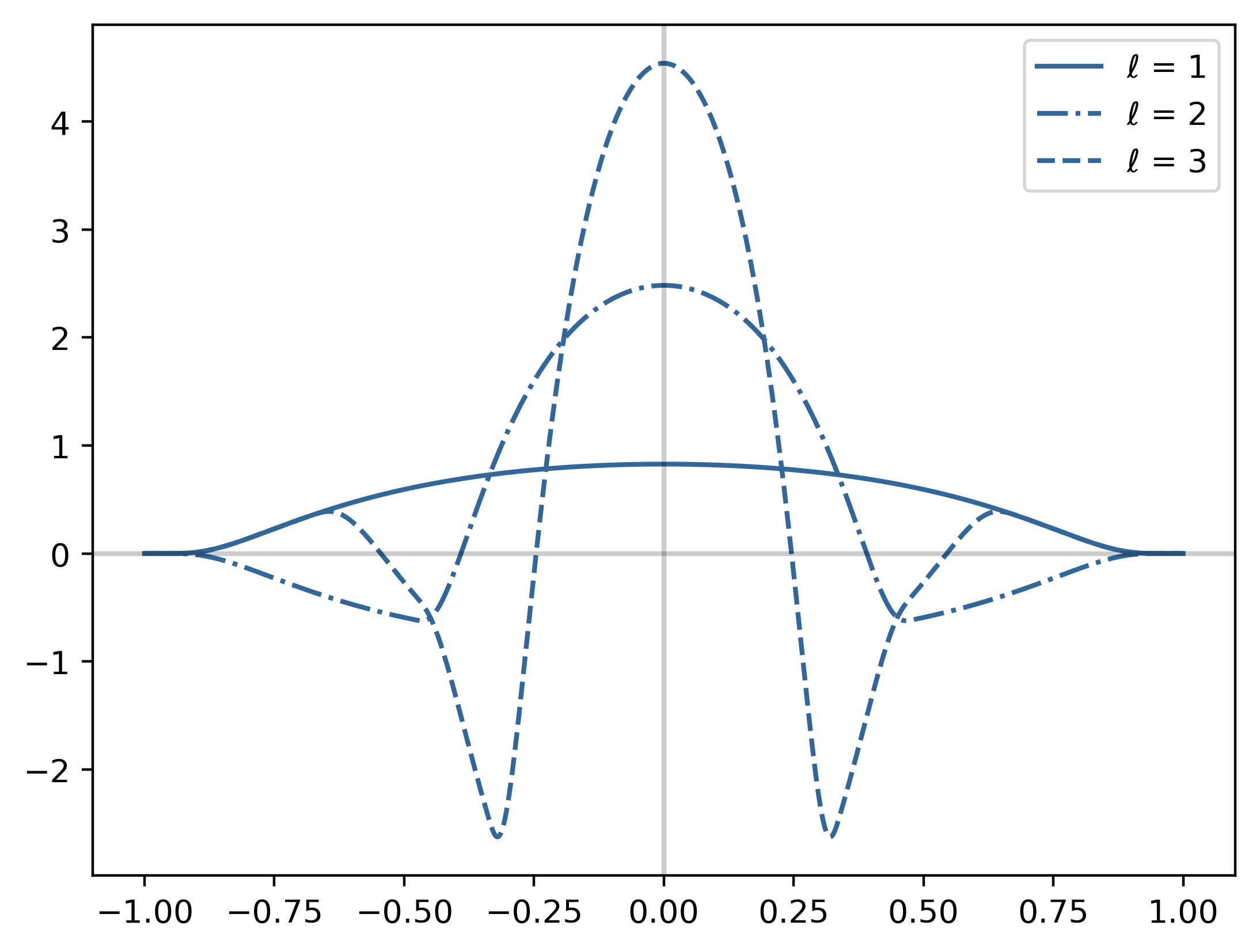
Figure 3: Plots of the kernel $K^{(d,\ell)}$ for $d=1$ and $\ell=1,2,3$.

Proposition 3.8.

Let $\ell$ be an integer greater than $\alpha$ and $\beta$, and let $K^{(\ell)}$ be the kernel defined in (6) starting from a kernel $K$ satisfying Assumption 3.6. Then, for any $P\in\Sigma^{d}_{\alpha,\beta}$ and any bandwidth $h<\tau/2$, the estimator $\widehat{f}_{h}(x)$ defined as in (3) using $K^{(\ell)}$ is such that

$$|\mathcal{B}_{h}(P,x)|\lesssim h^{\alpha\wedge\beta}.$$ (7)

Patching together Proposition 3.5 and Proposition 3.8 yields

$$\sup_{P\in\Sigma^{d}_{\alpha,\beta}}\mathbb{E}_{P^{\otimes n}}[|\widehat{f}_{h}(x)-f_{P}(x)|^{p}]^{1/p}\lesssim\Omega(h)+h^{\alpha\wedge\beta},$$

for any $h<\tau/2$. Therefore the estimator $\widehat{f}(x)=\widehat{f}_{h}(x)$ specified with $h=n^{-1/(2\alpha\wedge\beta+d)}$ indeed satisfies the conclusion of Theorem 3.1, for $n$ large enough.

3.3 A minimax estimator in the case $d=1$ that covers the case $\alpha<\beta$

The gap we observe between the two rates in Theorem 3.1 and Theorem 3.2 leads to the following question: does the regularity $\alpha\geq 0$ of $M$ have a genuine limiting effect in the estimation of $f(x)$, or does it rather reveal a weakness of the estimator described in Section 3.2. We do not have a definitive answer to this question except for $d=1$ i.e. when $M$ is a closed curve in an Euclidean space. We can then show that the parameter $\alpha$ does not interfere at all with the density estimation. The proofs of this section can be found in Appendix A.5.

If $d=1$, any submanifold $M$ in $\mathcal{C}_{1}(\tau)$ is a closed smooth injective curve that can be parametrized by a unit-speed path $\gamma_{M}:[0,L_{M}]\rightarrow\mathbb{R}^{D}$ with $\gamma_{M}(0)=\gamma_{M}(L_{M})$ and with $L_{M}=\operatorname{vol}M$ being the length of the curve. In that case, the volume density function is trivial.

Lemma 3.9.

For $M\in\mathcal{C}_{1}(\tau)$, for any $z\in M$ and any $v\in T_{z}M$, we have $\det g^{z}(v)=1$.

Thanks to Lemma 3.9, the estimator proposed by Pelletier (2005) takes a simpler form, which we will try to take advantage of. Indeed, in the representation (2) of Pelletier (2005), only $d_{M}$ remains unknown. We now show how to efficiently estimate $d_{M}$ thanks to the Isomap method as coined by Tenenbaum et al. (2000). The analysis of this algorithm essentially comes from Bernstein et al. (2000) and is pursued in Arias-Castro and Le Gouic (2019), but the bounds obtained there are manifold dependent. We thus propose a slight modification of their proofs in order to obtain uniform controls over $\mathcal{C}_{1}(\tau)$, and make use of the simplifications coming from the dimension $1$. Indeed, for $d=1$, we have the following simple and explicit formula for the intrinsic distance on $M$:

$$d_{M}(\gamma_{M}(s),\gamma_{M}(t))=|t-s|\wedge(L_{M}-|t-s|)~{}~{}~{}\forall s,t\in[0,L_{M}].$$

The Isomap method can be described as follows: let $\varepsilon>0$, and let $\mathcal{G}_{\varepsilon}$ be the $\varepsilon$-neighbourhood graph built upon the data $(X_{1},\dots,X_{n})$ and $x$ — namely, $\mathcal{G}_{\varepsilon}=(V,E)$ where $V=\left(x,X_{1},\dots,X_{n}\right)$, and where $E=\{(y,z)\in V~{}|~{}\|y-z\|\leq\varepsilon\}$. For a path in $\mathcal{G}_{\varepsilon}$ (meaning: a sequence of adjacent vertices) $s=(p_{0},\dots,p_{m})$, we define its length as $L_{s}=\|p_{1}-p_{0}\|+\dots+\|p_{m}-p_{m-1}\|$. The distance between $x$ and a vertice $y$ in the graph $\mathcal{G}_{\varepsilon}$ is then defined as

$$\widehat{d}_{\varepsilon}(x,y)=\min\big{\{}L_{s}~{}|~{}s~{}\text{path in}~{}\mathcal{G}_{\varepsilon}~{}\text{connecting $x$ to $y$}\big{\}},$$ (8)

and we set this distance to $\infty$ if $x$ and $y$ are not connected. We are now ready to describe our estimators $\hat{f}^{\operatorname{1D}}(x)$. For any $h,\varepsilon>0$, we set

$$\hat{f}_{h}^{\operatorname{1D}}(x)=\frac{1}{nh}\sum_{i=1}^{n}K^{\operatorname{1D}}\big{(}\widehat{d}_{\varepsilon}(x,X_{i})/h\big{)},$$ (9)

for some kernel $K^{\operatorname{1D}}:\mathbb{R}\rightarrow\mathbb{R}$. Notice that the kernel $K^{(1,\ell)}(\cdot):\mathbb{R}^{D}\rightarrow\mathbb{R}$ defined in Section 3.2 starting from kernel $K=\lambda_{1}^{-1}\Lambda$ can be put in the form $K^{(1,\ell)}(y)=K^{(1,\ell)}(\|y\|)$ with $K^{(1,\ell)}(\cdot)$ denoting thus (with a slight abuse of notation) both functions starting from either $\mathbb{R}$ or $\mathbb{R}^{D}$. We choose this kernel in the next statement.

Proposition 3.10.

Assume that $f_{\min}>0$. The estimator defined in (9) above and specified with $K^{\operatorname{1D}}=K^{(1,\ell)}(\cdot)$ satisfies the following property: for any $\beta\in[0,\ell]$ and any $\alpha\geq 0$, we have

$$\sup_{P\in\Sigma_{\alpha,\beta}^{1}}\mathbb{E}_{P^{\otimes n}}[|\hat{f}^{\operatorname{1D}}_{h}(x)-f_{P}(x)|^{p}]^{1/p}\lesssim\frac{\varepsilon^{2}}{h^{2}}+\Omega(h)+h^{\beta}+\frac{1}{nh}~{}~{}~{}~{}\text{with}~{}~{}~{}\varepsilon=\frac{32(p+1)}{f_{\min}}\times\frac{\log n}{n},$$

for $h<\tau/4$ and $n$ large enough.

The proof of Theorem 3.3 readily follows from Proposition 3.10 using the estimator $\hat{f}^{\operatorname{1D}}=\hat{f}^{\operatorname{1D}}_{h}$ with $h=n^{-1/(2\beta+1)}$.

3.4 Smoothness adaptation

We implement Lepski’s algorithm, following closely Lepski et al. (1997) in order to automatically select the bandwidth from the data $(X_{1},\ldots,X_{n})$. We know from Section 3.2 that the optimal bandwidth on $\Sigma^{d}_{\alpha,\beta}$ is of the form $n^{-1/(2\alpha\wedge\beta)+d}$. Hence, without prior knowledge of the value of $\alpha$ and $\beta$, we can restrict our search for a bandwidth in a bounded interval of the form $[h^{-},1]$ discretized as follow

$$\mathbb{H}=\big{\{}2^{-j},~{}~{}\text{for}~{}~{}0\leq j\leq\log_{2}(1/h^{-})\big{\}}$$

We choose to pick

$$h^{-}=\left(\frac{\|K\|_{\infty}}{2\omega}\right)^{1/d}\frac{1}{n^{1/d}};$$

this bandwidth is always smaller than the optimal bandwidth $n^{-1/(2\alpha\wedge\beta+d)}$ on $\Sigma^{d}_{\alpha,\beta}$ for $n$ large, and is such that $\Omega(h)\leq 2\sqrt{2\omega/(nh^{d})}$ for all $h\geq h^{-}$. For $h,\eta\in\mathbb{H}$, we introduce the following quantities:

$$\lambda(h) =1\vee\sqrt{\Theta d\log(1/h)},$$

$$\psi(h,\eta) =\Omega(h)\lambda(h)+\Omega(\eta)\lambda(\eta)$$ (10)

where $\Theta$ is a positive constant (to be specified). For $h\in\mathbb{H}$ we define the subset of bandwidths $\mathbb{H}(h)=\{\eta\in\mathbb{H},~{}\eta\leq h\}$ The selection rule for $h$ is the following:

$$\widehat{h}(x)=\max\Big{\{}h\in\mathbb{H}~{}|~{}\forall\eta\in\mathbb{H}(h),~{}|\widehat{f}_{h}(x)-\widehat{f}_{\eta}(x)|\leq\psi(h,\eta)\Big{\}},$$

and we finally consider the estimator

$$\widehat{f}(x)=\widehat{f}_{\widehat{h}(x)}(x).$$ (11)

where we recall that $f_{h}$ is defined at (3).

Proposition 3.11.

Assume $\Theta>p$. Let $\ell\in\mathbb{N}$, and let $\widehat{f}(x)$ be the estimator defined in (11) using $K^{(\ell)}$ originated from a kernel $K$ satisfying Assumption 3.6. Then, for any $\alpha,\beta\in[0,\ell]$, we have, for $n$ large enough

$$\sup_{P\in\Sigma^{d}_{\alpha,\beta}}\mathbb{E}_{P^{\otimes n}}[|\widehat{f}(x)-f_{P}(x)|^{p}]^{1/p}\lesssim\left(\frac{\log n}{n}\right)^{\alpha\wedge\beta/(2\alpha\wedge\beta+d)}.$$

The proof of Proposition 3.11 can be found in Appendix A.6. Some remarks: 1) Proposition 3.11 provides us with a classical smoothness adaptation result in the spirit of (Lepski et al., 1997): the estimator $\widehat{f}$ has the same performance as the estimator $\widehat{f}_{h}$ selected with the optimal bandwidth $n^{-1/(2\alpha\wedge\beta+d)}$, up to a logarithmic factor on each model $\Sigma^{d}_{\alpha,\beta}$ without the prior knowledge of $\alpha\wedge\beta$ over the range $[0,\ell]$. 2) The extra logarithmic term is the unavoidable payment for the Lepski-Low phenomenon Lepskiĭ (1990); Low (1992) when recovering a function in pointwise or in a uniform loss.

3.5 Simultaneous adaptation to smoothness and dimension

The estimators considered in Theorem 3.1 or Proposition 3.11 heavily rely on the intrinsic dimension $d$ through the choice a of kernel satisfying Assumption 3.6, through the normalization $h^{d}$ and either through the choice of an optimal bandwidth $h$, or the selection procedure (10)-(11). We now show how to adapt to $d$ considered as an unknown and nuisance parameter.The proofs of this section can be found in Appendix A.7.

We redefine all the quantities introduced before as now depending on $d$. Namely, for $h,\eta>0$, and a given family of kernel $K(d;\cdot)$, we set

$$\widehat{f}_{h}(d;x) =\frac{1}{nh^{d}}\sum_{i=1}^{n}K(d;(X_{i}-x)/h).$$

$$\Omega(d;h) =\sqrt{\frac{2\omega_{d}}{nh^{d}}}+\frac{\|K(d;\cdot)\|_{\infty}}{nh^{d}}~{}~{}~{}\text{with}~{}~{}~{}\omega_{d}=4^{d}\zeta_{d}\|K(d;\cdot)\|_{\infty}^{2}f_{\max},$$

$$\lambda(d;h) =1\vee\sqrt{\Theta d\log(1/h)},$$

$$\psi(d;h,\eta) =v(d;h)\lambda(d;h)+v(d;\eta)\lambda(d;\eta),$$

$$h^{-}_{d} =(\|K(d;\cdot)\|_{\infty}/2\Omega_{d})^{1/d}n^{1/d},$$

$$\mathbb{H}_{d} =\{2^{-j},~{}\text{for}~{}~{}0\leq j\leq\log_{2}(1/h_{d}^{-})\},$$

where $\Theta$ is a constant. We also define

$$\widehat{h}(d;x)=\max\{h\in\mathbb{H}_{d}~{}|~{}\forall\eta\in\mathbb{H}_{d}(h),~{}~{}|\widehat{f}_{h}(d;x)-\widehat{f}_{\eta}(d;x)|\leq\psi(d;h,\eta)\}$$ (12)

with $\mathbb{H}_{d}(h)=\{\eta\in\mathbb{H}_{d},~{}\eta\leq h\}$. We are now left with the choice of kernel family $K(d;\cdot)$. For any $1\leq d\leq D-1$ and $h>0$, we define

$$K^{(1)}(d;x)=\lambda_{d}^{-1}\Lambda(x)$$

where $\Lambda$ and $\lambda_{d}$ have been introduced in Section 3.2. We then pick an integer $\ell\in\mathbb{N}$ and choose

$$K(d;\cdot)=K^{(d,\ell)}(d;\cdot)$$ (13)

where $K^{(d,\ell)}(d;\cdot)$ is defined by recursion in (6) starting from the kernel $K^{(1)}(d;\cdot)$.

We assume that we have an estimator $\widehat{d}$ of the dimension $d$ of $M$ with values in $\{1,\dots,D\}$. More precisely, we require the following property

Assumption 3.12.

For any $1\leq d<D$ and all real numbers $\alpha,\beta\in[0,\ell]$, we have

$$\sup_{P\in\Sigma^{d}_{\alpha,\beta}}P^{\otimes n}\left(\widehat{d}\neq d\right)\lesssim n^{-3p/2}.$$

If we are given such a estimator of the dimension $d$, then we can built a estimator that adapts to this parameter.

Proposition 3.13.

Let $\widehat{f}(x)=\widehat{f}_{\widehat{h}}(\widehat{d},x)$ built with the kernel family (13), where $\widehat{d}$ is a estimator satisfying Assumption 3.12 and where $\widehat{h}=\widehat{h}(\widehat{d},x)$ is defined at (12). Then, for any $1\leq d\leq D-1$, and any $\alpha,\beta\in[0,\ell]$, we have, for $n$ large enough

$$\sup_{P\in\Sigma^{d}_{\alpha,\beta}}\mathbb{E}_{P^{\otimes n}}[|\widehat{f}(x)-f_{P}(x)|^{p}]^{1/p}\lesssim\left(\frac{\log n}{n}\right)^{\alpha\wedge\beta/(2\alpha\wedge\beta+d)}$$

It only remains to show that there exists an estimator $\widehat{d}$ satisfying Assumption 3.12 to obtain Theorem 3.4. There are various way to define such an estimator, see Farahmand et al. (2007) or even Kim et al. (2016) where an estimator with super-exponential minimax rate on a wide class of probability measures is constructed. For sake of completeness and simplicity, we will mildly adapt the work of Farahmand et al. (2007) to our setting. The resulting estimator will behave well as soon as we add the assumption that $f_{\min}>0$.

Definition 3.14.

For a probability measure $P$, we write $P_{\eta}=P(B(x,\eta))$ for any $\eta>0$, and $\widehat{P}_{\eta}=\widehat{P}_{n}(B(x,\eta))$ where $\widehat{P}_{n}=n^{-1}\sum_{i=1}^{n}\delta_{X_{i}}$ denotes the empirical measure of the sample $(X_{1},\ldots,X_{n})$. Define

$$\widehat{\delta}_{\eta}=\log_{2}\widehat{P}_{2\eta}-\log_{2}\widehat{P}_{\eta},$$

and set $\widehat{\delta}_{\eta}=D$ when $\widehat{P}_{\eta}=0$. We define $\widehat{d}_{\eta}$ to be the closest integer of $\{1,\dots,D\}$ to $\widehat{\delta}_{\eta}$, namely $\widehat{d}_{\eta}=\lfloor\widehat{\delta}_{\eta}+1/2\rfloor$.

Proposition 3.15.

Assume that $f_{\min}>0$. Then, for any $1\leq d\leq D-1$, and any $\alpha,\beta\geq 0$, the estimator $\widehat{d}=\widehat{d}_{\eta}$ for $\eta=n^{-1/(2D+2)}$ verifies for $n$ large enough

$$\sup_{P\in\Sigma^{d}_{\alpha,\beta}}P^{\otimes n}\left(\widehat{d}\neq d\right)\leq 4\exp\left(-2n^{1-(d+1)/(D+1)}\right).$$

4 Numerical illustration

In this section we propose a few simulations to illustrate the results presented above. The goal is two-fold

• To highlight the rate obtained in Theorem 3.1 using estimator $\widehat{f}_{h}$, in the case where $\beta\leq\alpha$, on arbitrary submanifold and for a carefully chosen bandwidth $h$;

• To show the computational feasability and performance of estimator $\hat{f}^{\operatorname{adapt}}$ described in Section 3.4.

For the sake of visualisation and simplicity, we focus on two typical examples of submanifold of $\mathbb{R}^{D}$, namely non-isometric embeddings of the flat circle $\mathbb{T}^{1}=\mathbb{R}/\mathbb{Z}$ and of the flat torus $\mathbb{T}^{2}=\mathbb{T}^{1}\times\mathbb{T}^{1}$. In particular, these embeddings will be chosen in such way that their images, as submanifolds of $\mathbb{R}^{D}$, are not homogeneous compact Riemannian manifolds, so that the work of Kerkyacharian et al. (2012) for instance cannot be of use here.

For a given embedding $\Phi:N\rightarrow M\subset\mathbb{R}^{D}$ where $N$ is either $\mathbb{T}^{1}$ of $\mathbb{T}^{2}$, we construct absolutely continuous probabilities on $M$ by pushing forward probability densities of $N$ w.r.t. their volume measure. Indeed, if $Q=g\cdot\mu_{N}$, the push-forward measure $P=\Phi_{*}Q$ has density $f$ with respect to $\mu_{M}$ given by

$$\forall z\in M,~{}~{}~{}f(z)=\frac{g(\Phi^{-1}(z))}{\left|\det d\Phi(\Phi^{-1}(z))\right|}$$ (14)

where the determinant is taken in an orthonormal basis of $T_{\Phi^{-1}(x)}N$ and $T_{x}M$, so that, if $\Phi$ is chosen smooth enough, $f$ has the same regularity as $g$. If $\Phi$ is an embedding of $\mathbb{T}^{1}$, we simply have $\left|\det d\Phi(y)\right|=\|\Phi^{\prime}(y)\|$ for all $y\in\mathbb{T}^{1}$. If now $\Phi$ maps $\mathbb{T}^{2}$ to $M$, we have

$$\left|\det d\Phi(y)\right| =\sqrt{\det\langle d\Phi(y)[e_{i}],d\Phi(y)[e_{j}]\rangle_{1\leq i,j\leq 2}}$$

$$=\sqrt{\left\|d\Phi(y)[e_{1}]\right\|^{2}\left\|d\Phi(y)[e_{2}]\right\|^{2}-\langle d\Phi(y)[e_{1}],d\Phi(y)[e_{2}]\rangle^{2}}$$ (15)

where $(e_{1},e_{2})$ is an orthonormal basis of $\mathbb{R}^{2}\simeq T_{y}\mathbb{T}^{2}$.

Strictly speaking, the probability measures $P$ exhibited below are not elements of the models $\Sigma^{d}_{\alpha,\beta}$, but we know that they locally coincide with some $\widetilde{P}\in\Sigma^{d}_{\alpha,\beta}$ around our candidate point $x$, meaning that

$$P_{|B(x,r)}=\widetilde{P}_{|B(x,r)}~{}~{}~{}\text{for some}~{}~{}r>0.$$

This ensures that all the results displayed in Section 3 hold for $P$ — see Remark 2.2 for a discussion on the local character of our setting.

4.1 An example of a density supported by a one-dimensional submanifold

Let $\beta\in\mathbb{N}^{*}$ and define the following function for $v\in[-1/2,1/2]$

$$g_{\beta}(v)=C_{\beta}\times\left(1-(-2v)^{\beta}\right)\mathbbm{1}_{[-1/2,0)}(v)+C_{\beta}\left(1-(2v)^{\beta+1}\right)\mathbbm{1}_{[0,1/2]}.$$ (16)

where $C_{\beta}$ is an explicit normalisation constant. The function $g_{\beta}$ is positive and $\int_{0}^{1}g_{\beta}(v)dt=1$; it defines a probability density over [-1/2,1/2]. Also, because the $(\beta-1)$-th derivative of $g_{\beta}$ is $1$-Lipschitz, but its $\beta$-derivative is discontinuous at $v=0$, the function $g_{\beta}$ is $\beta$-Hölder but not $(\beta+\varepsilon)$-Hölder for any $\varepsilon>0$. See Figure 4 for a few plots of the functions $g_{\beta}$.

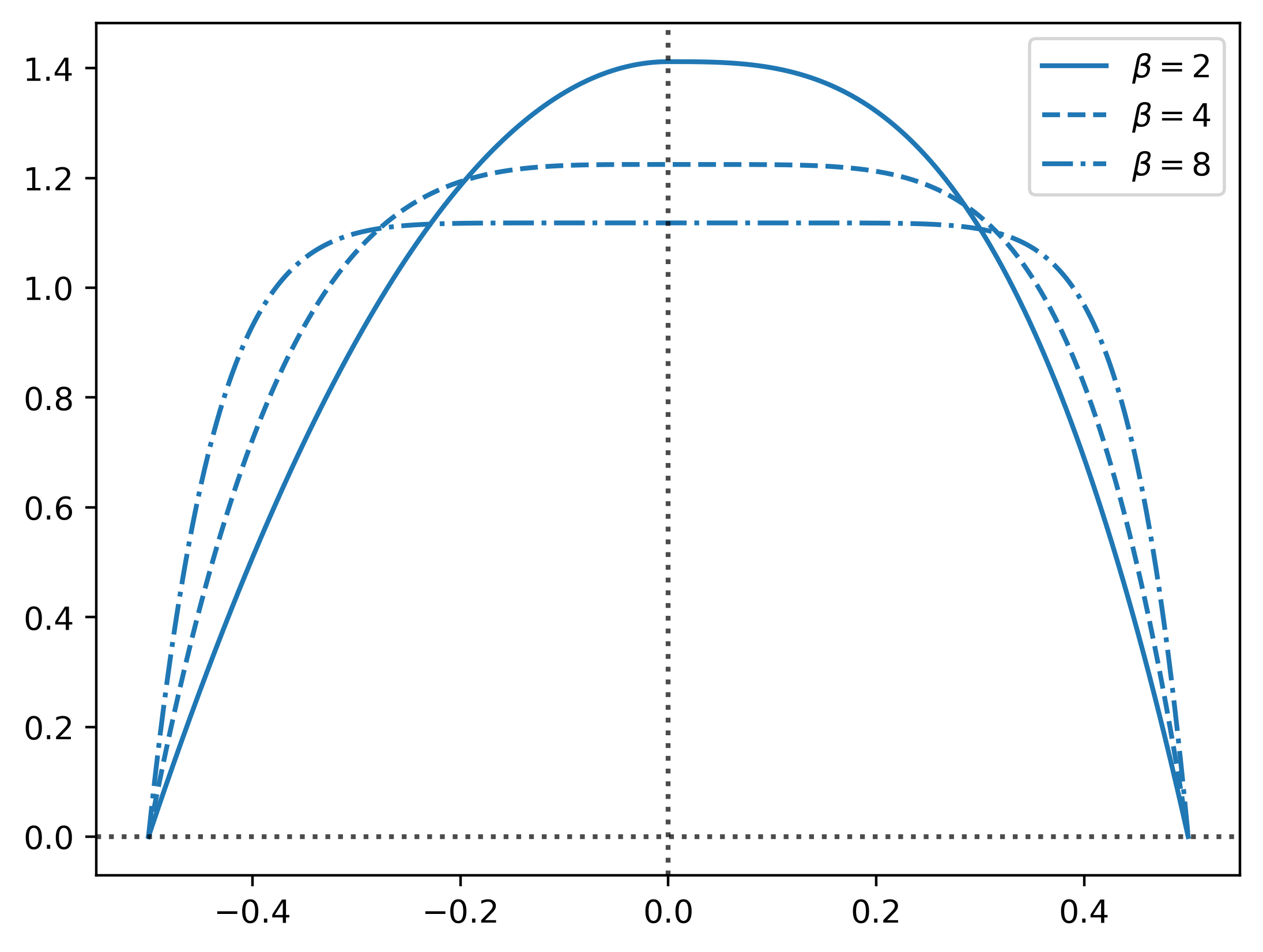
Figure 4: Plots of the densities $g_{\beta}$ for $\beta=2,4,8$.

We next consider the parametric curve

$$\Phi:\begin{cases}\mathbb{T}^{1}\rightarrow\mathbb{R}^{2}\\ t\mapsto\left(\cos(2\pi v)+a\cos(2\pi\omega v),\sin(2\pi v)+a\sin(2\pi\omega v)\right).\end{cases}$$

Short computations show that $\Phi$ is indeed an embedding as soon as $a\omega<1$, in which case $M=\Phi(\mathbb{T}^{1})$ is indeed a smooth compact submanifold of $\mathbb{R}^{2}$. For the rest of this section, we set $a=1/8$ and $\omega=6$. See Figure 5 for a plot of $M$ with these parameters.

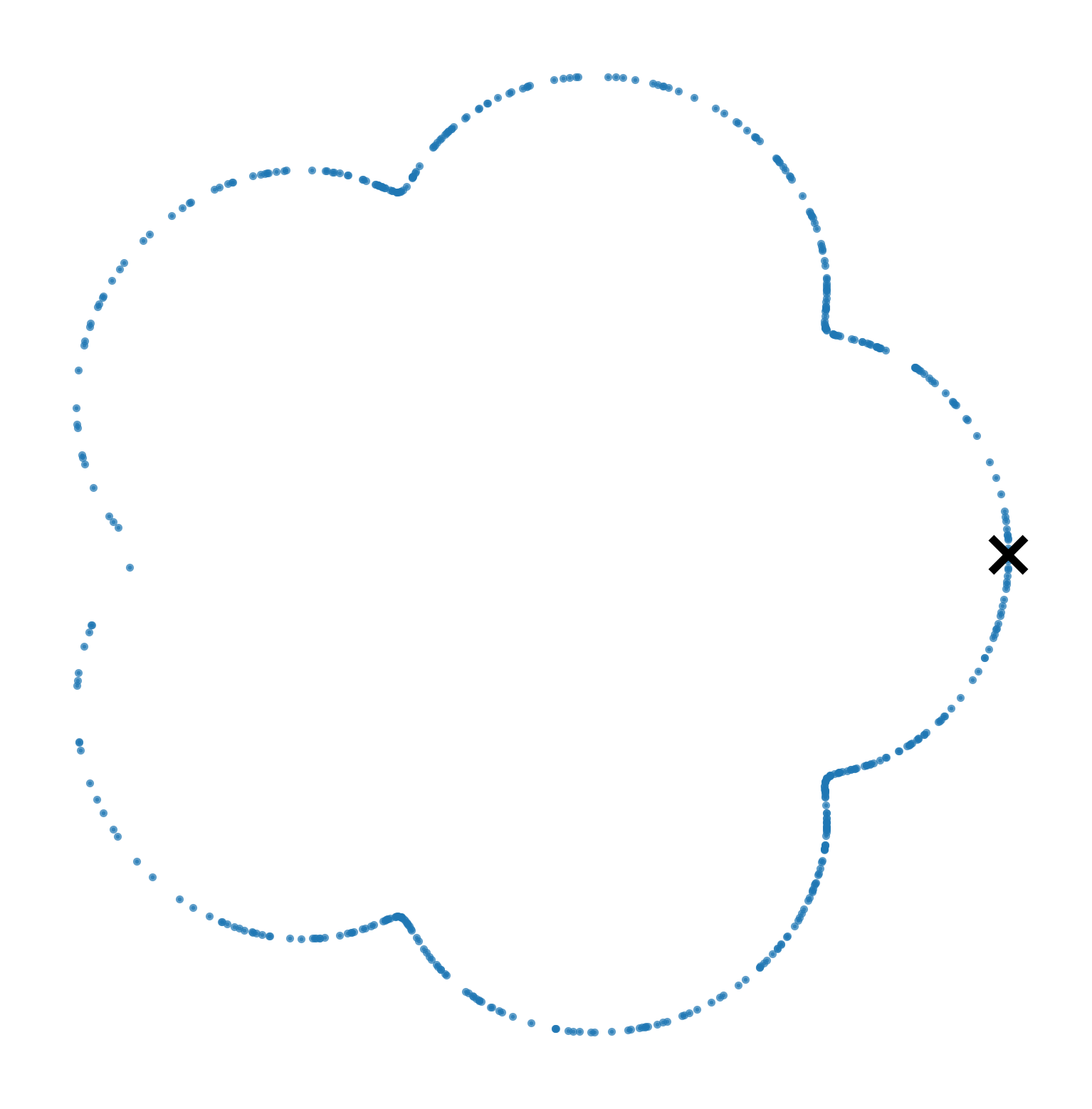
Figure 5: Plot of the submanifold M (Left) for parameters $a=1/8$ and $\omega=6$, and 500 points sampled independently from $\Phi_{*}g_{\beta}\cdot\mu_{\mathbb{T}^{1}}$ for $\beta=3$ (Right). The black cross denotes the point $x=\Phi(0)$.

We are interested in estimating the density $f_{\beta}$ with respect to $d\mu_{M}$ of the push-forward measure $P_{\beta}=\Phi_{*}g_{\beta}\cdot\mu_{\mathbb{T}^{1}}$, at point $x=(1+a,0)\in M$. We use formula (14) to compute $f_{\beta}(x)$: We have $\Phi^{-1}(x)=0$ and $\|\Phi^{\prime}(0)\|=2\pi(1+a\omega)$ hence

$$f_{\beta}(x)=\frac{C_{\beta}}{2\pi(1+a\omega)}\;\;\text{at}\;\;x=(1+a,0).$$

Our aim here is to provide an empirical measure for the convergence of the risk $n\mapsto\mathbb{E}_{{P_{\beta}}^{\otimes n}}[|\widehat{f}_{h}(x)-f_{\beta}(x)|^{p}]^{1/p}$ when $h$ is tuned optimally (in an oracle way). We pick $p=2$. Our numerical procedure is detailed in Algorithm 1 below, and the numerical results are presented in Figure 8.

Algorithm 1 MSE rate of convergence estimation

1:Provide integers $\beta\geq 1$ and $\ell\geq\beta$.

2:Set a grid of increasing number of points $\mathbf{n}=(n_{1},\dots,n_{k})\in\mathbb{N}^{k}$ and a number of repetition $N$.

3:for $n_{i}\in\mathbf{n}$ do

4:     Sample $n_{i}$ points independently from $P_{\beta}$,

5:     Compute $\widehat{f}_{h_{i}}(x)$ with kernel $K^{(\ell)}$ and bandwidth $h_{i}=n_{i}^{-1/(2\beta+1)}$,

6:     Compute the square error $(\widehat{f}_{h_{i}}(x)-f_{\beta}(x))^{2}$,

7:     Repeat the three previous steps $N$ times,

8:     Average the errors to get a Monte-Carlo approximation $\widehat{R}(n_{i})$ of $\mathbb{E}_{{P_{\beta}}^{\otimes n_{i}}}[|\widehat{f}_{h}(x)-f_{\beta}(x)|^{2}]$.

9:end for

10:Perform an Ordinary Least Square Linear Regression on the curve $\log n_{i}\mapsto\log\widehat{R}(n_{i})$.

11:return The coefficient of the linear regression.

4.2 An example of a density supported by a two-dimensional submanifold

We consider a non-isometric embedding of the flat torus $\mathbb{T}^{2}$. We first construct a density function. For and integer $\beta\geq 1$, define

$$G_{\beta}:(v,u)\in[-1/2,1/2]^{2}\mapsto g_{\beta}(v)g_{\beta}(u)\noindent$$ (17)

where $g_{\beta}$ is defined as in (16). Obviously, $G_{\beta}$ defines a density function on $\mathbb{T}^{2}$ that is $\beta$-Hölder (but not $(\beta+\varepsilon)$-Hölder for any $\varepsilon>0$).

Figure 6: Plot of the probability density function $G_{\beta}$ for $\beta=3$.

We next consider the parametric surface

$$\Psi:\begin{cases}\mathbb{T}^{2}\rightarrow\mathbb{R}^{3}\\ (v,u)\mapsto\begin{pmatrix}(b+\cos(2\pi v))\cos(2\pi u)+a\sin(2\pi\omega v)\\ (b+\cos(2\pi v))\sin(2\pi u)+a\cos(2\pi\omega v)\\ \sin(2\pi v)+a\sin(2\pi\omega u)\end{pmatrix}\end{cases}$$

for some $a,b,\omega\in\mathbb{R}$. In the remaining of the section, we set $a=1/8$, $b=3$ and $\omega=5$. We show that $\Phi$ indeed defines an embedding. See Figure 7 for a plot of the submanifold $M=\Psi(\mathbb{T}^{2})$. For an integer $\beta\geq 1$, we denote by $F_{\beta}$ the density of the push forward measure $Q_{\beta}=\Psi_{*}G_{\beta}\cdot\mu_{\mathbb{T}^{2}}$ with respect to the volume measure $\mu_{M}$. Let $x=(b+1,a,0)$ be the image of $0$ by $\Psi$.

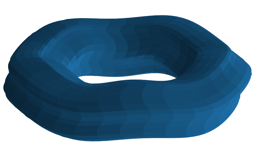
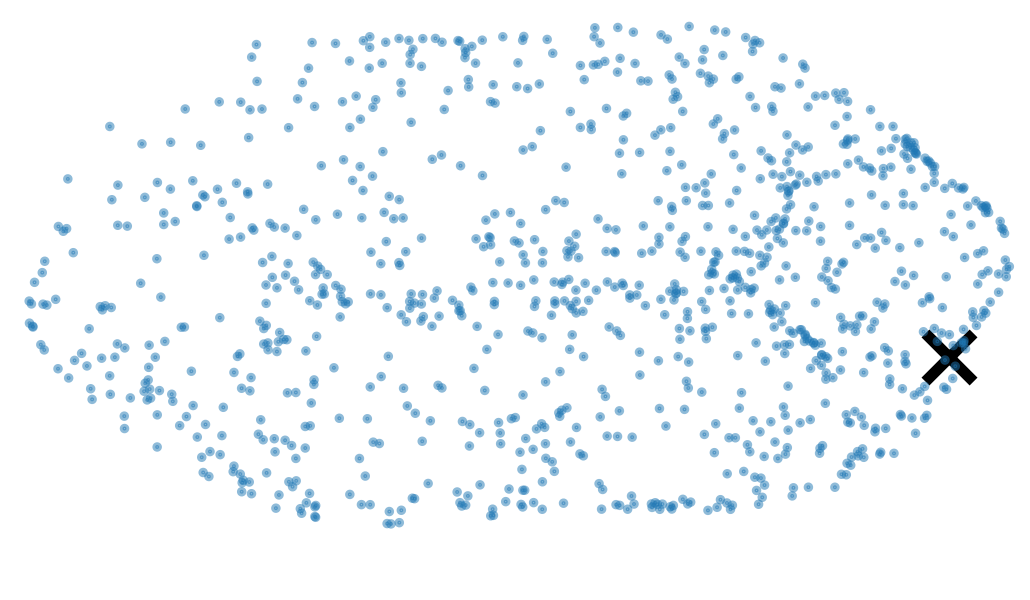
Figure 7: Plot of the submanifold $M$ (Left) for parameters $a=1/8$, $b=3$ and $\omega=6$, and 500 points sampled independently from $\Psi_{*}G_{\beta}\cdot\mu_{\mathbb{T}^{2}}$ with $\beta=3$ (Right). The black cross marks the point $x$.

Simple calculations show that the differential of $\Psi$ at $0$ evaluated at $e_{1}=(1,0)\in T_{0}\mathbb{T}^{2}$ and $e_{2}=(0,1)\in T_{0}\mathbb{T}^{2}$ is equal to respectively $d\Psi(0)[e_{1}]=2\pi(a\omega,0,1)$ and $d\Psi(0)[e_{2}]=2\pi(0,b+1,a\omega)$. Hence formula (4) yields

$$\det d\Psi(0)=(2\pi)^{2}\left(\left(1+a^{2}\omega^{2}\right)\left((b+1)^{2}+a^{2}\omega^{2}\right)-a^{2}\omega^{2}\right)^{1/2}$$ (18)

and we obtain

$$F_{\beta}(x)=\frac{C_{\beta}^{2}}{4\pi^{2}}\left(\left(1+a^{2}\omega^{2}\right)\left((b+1)^{2}+a^{2}\omega^{2}\right)-a^{2}\omega^{2}\right)^{-\frac{1}{2}}.$$

In the same way as in the previous section, we aim at providing an empirical measure for the rate of convergence of the risk $\mathbb{E}_{{P_{\beta}}^{\otimes n}}[|\widehat{f}_{h}(x)-f_{\beta}(x)|^{2}]$ when $h$ is suitably tuned with respect to $n$ and $\beta$. This is done using again Algorithm 1. The results are presented in Figure 8.

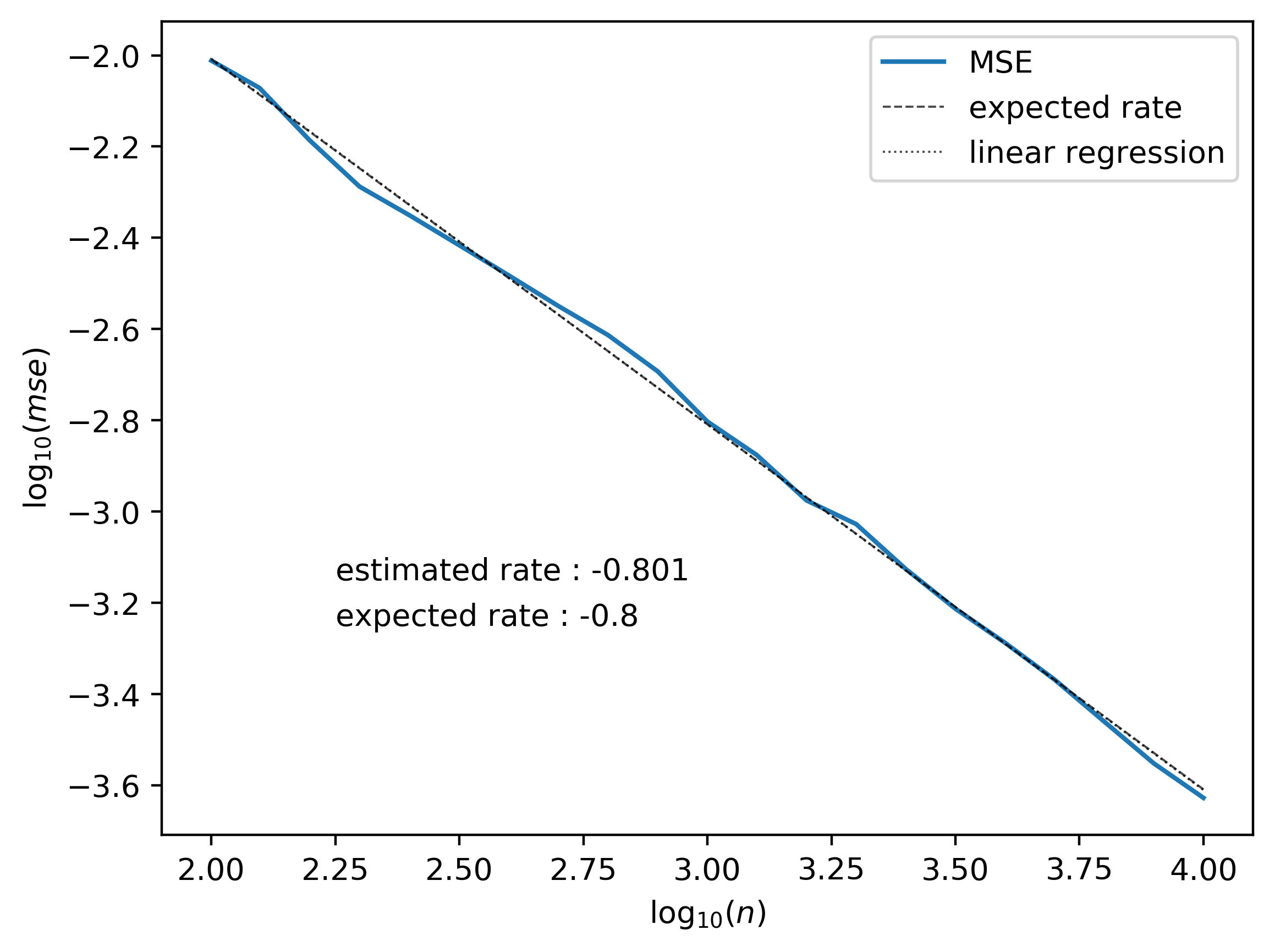
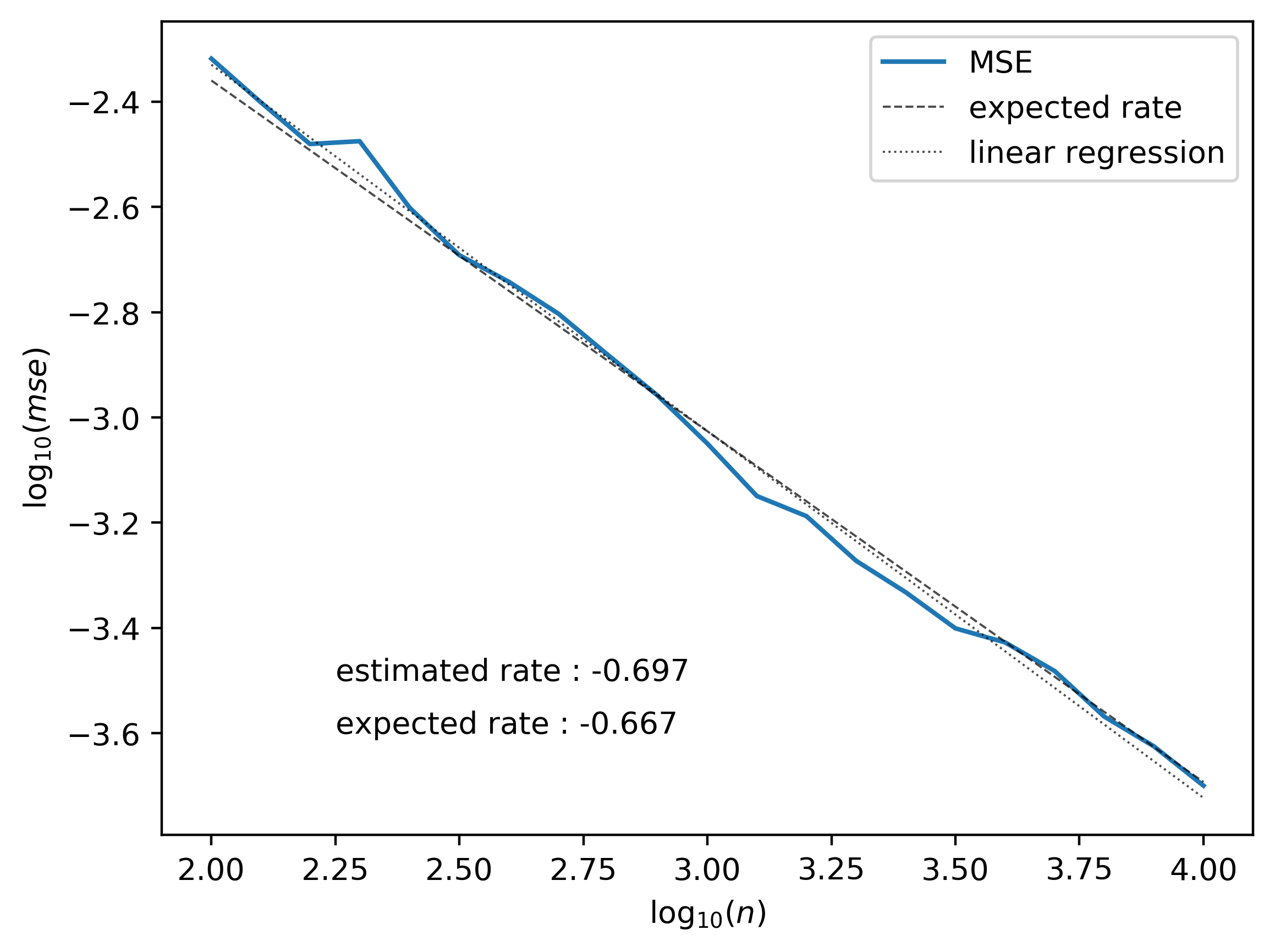
Figure 8: Plot of the empirical mean square error (blue) for a density supported by a one-dimensional submanifold (Left) and two-dimensional submanifold (Right) with parameter $\beta=2$. We use a log-regular grid $\mathbf{n}$ of $21$ points ranging from $100$ to $10^{4}$. Each experiment is repeated $N=500$ times.

4.3 Adaptation

In this section we estimate a density when its regularity is unknown, contrary to the previous simulation where the regularity parameter $\beta$ is pugged in the bandwidth choice $n^{-1/(2\beta+d)}$. This is performed using Lepski’s method presented in Section 3.4. The rate is computed using Algorithm 1, for both the one-dimensional and the two-dimensional synthetic datasets.

For the adaptive estimation on the two-dimensional manifold, we observe that the corrective term $\det d\Psi(0)$ computed in (18) results in a density $F_{\beta}(x)$ that is quite small, while the function $\psi$ defined at (10) and used to tune the bandwidth soars dramatically because of the retained value of $\omega_{d}=4^{d}\zeta_{d}\|K^{(d,\ell)}\|^{2}_{\infty}f_{\max}$, so that the values of $\hat{f}_{h}$ and $\psi(h,\cdot)$ (defined at (10)) are not of the same order anymore at this scale (using maximum $10^{6}$ observations). To circumvent this effect, we introduce a scaling parameter $\lambda$ as follows

$$G_{\beta,\lambda}=v,u\mapsto\lambda^{2}G_{\beta}(\lambda v,\lambda u).$$

Like before, we consider the push-forward probability measure $\Psi_{*}G_{\beta,\lambda}\cdot\mu_{\mathbb{T}^{2}}$ which has density $F_{\beta,\lambda}$ with respect to $\mu_{M}$. For $\lambda=4$, we find that $F_{\beta,\lambda}(x)$ is of order $1$ for most values of $\beta$, and we use the function $\psi^{\text{num}}(h,\eta)=\Omega^{\text{num}}(h)\lambda(h)+\Omega^{\text{num}}(\eta)\lambda(\eta)$ using simply $\Omega^{\text{num}}(h)=\sqrt{1/nh^{d}}$. We have no theoretical guarantee that such a method will work but we recover nonetheless the right rate in the estimation of the value of the density, see Figure 9 for a plot of the estimated rate.

We find a highly dispersive empirical error, hence our choice to represent the median of the squared error instead of the more traditional mean squared error.

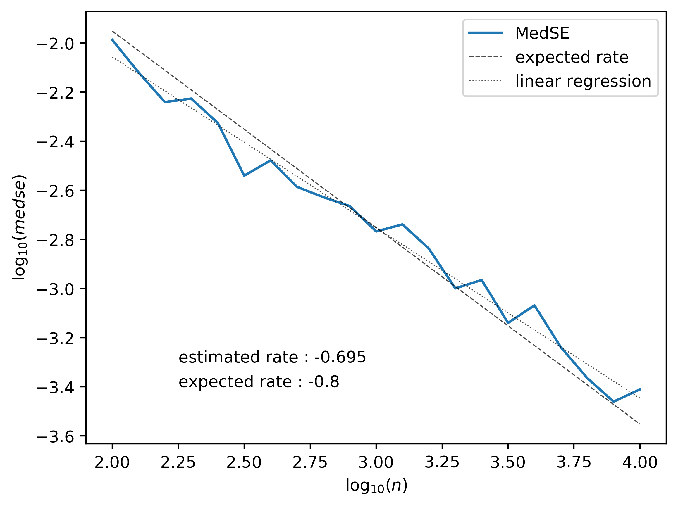
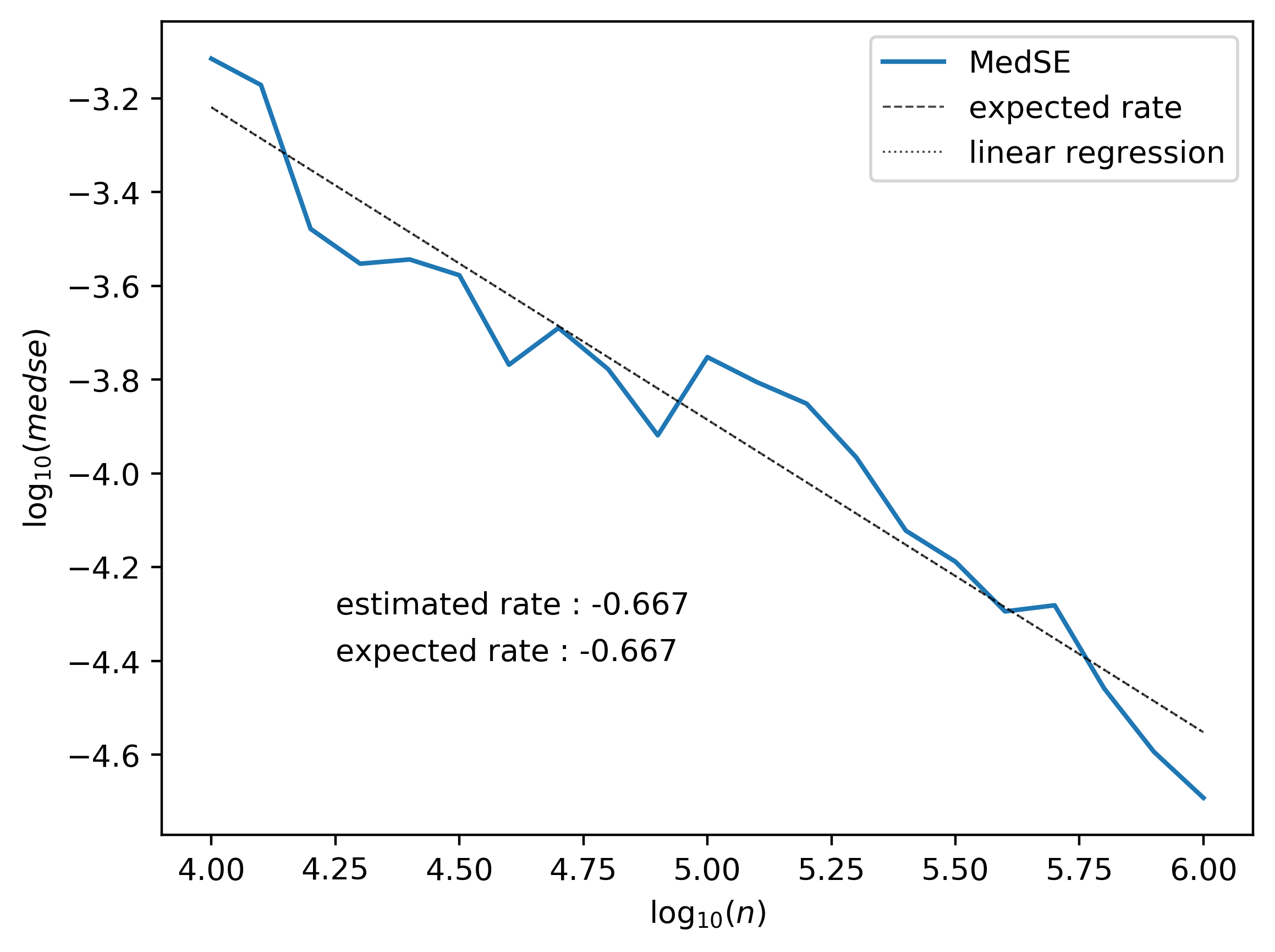
Figure 9: (Left) Plot of the empirical median square error for the one-dimensional submanifold with $\beta=2$. The bandwidth $h$ is chosen adaptively using Lepski’s method of order $\ell=3$ as in Section 3.4. We used a log-regular grid $\bf n$ of $11$ points ranging from $100$ to $10^{4}$ and each experience was repeated $N=500$ times. (Right) Same experiment but for the two dimensional manifold, with a grid ranging from $10^{4}$ to $10^{6}$ and $N=100$ repetitions.

Acknowledgements We are grateful to Krishnan (Ravi) Shankar and Hippolyte Verdier for insightful discussions and comments. The valuable input of two referees is greatly acknowledged.

A Appendix

A.1 Additional results of geometry

We first state a few classical results that we will need in the upcoming proofs. We start with a quantitative bound that link the reach to the curvature of a submanifold. We denote by $\operatorname{I\!I}$ the second fundamental form.

Proposition A.1.

(Niyogi et al., 2008, Prp. 6.1) Let $M$ be a compact smooth submanifold of $\mathbb{R}^{D}$. Then, for any $z\in M$, we have $\|\operatorname{I\!I}_{z}\|_{\operatorname{op}}\leq 1/\tau_{M}$.

Since $\operatorname{I\!I}_{z}$ is the differential of order two of the mapping $\exp_{z}$ at the $0\in T_{x}M$, Proposition A.1 has several convenient implications. First, it gives a uniform lower bound for the injectivity radii of $M$ as stated in Proposition 2.3. Second, it also yields nice bounds on how well the Euclidean distance on $\mathbb{R}^{D}$ approximates the Riemannian distance $d_{M}$ on $M\times M$.

Proposition A.2.

(Niyogi et al., 2008, Prp. 6.3) For any compact submanifold $M$ of $\mathbb{R}^{D}$ and any $x,y\in M$ such that $\|x-y\|\leq\tau_{M}/2$, we have

$$\|x-y\|\leq d_{M}(x,y)\leq\tau_{M}\left(1-\sqrt{1-\frac{2\|x-y\|}{\tau_{M}}}\right).$$

Proposition A.2 allows in turn to compare the volume measure $\mu_{M}$ to the Lebesgue measure on its tangent spaces.

Lemma A.3.

For any $d$-dimensional compact smooth submanifold $M$ of $\mathbb{R}^{D}$, for any $z\in M$ and any $\eta\leq\tau_{M}/2$, we have

$$(1-\eta^{2}/6\tau_{M}^{2})^{d}\zeta_{d}\eta^{d}\leq\mu_{M}(B(z,\eta))\leq\{(1+(\xi(\eta/\tau_{M})\eta)^{2}/\tau_{M}^{2})\xi(\eta/\tau_{M})\}^{d}\zeta_{d}\eta^{d}$$

where $\xi(s)=(1-\sqrt{1-2s})/s$ and $\zeta_{d}$ is the volume of the unit Euclidean ball in $\mathbb{R}^{d}$.

Proof.

This result already appears in (Aamari, 2017, Lem III.23) but we prove it here to make constants explicit. Let us denote by $\operatorname{Leb}$ the Lebesgue measure on $T_{x}M$. Using (Aamari, 2017, Prp III.22.v), we know that, as long as $\xi(\eta/\tau_{M})\eta\leq\tau_{M}$ (which holds if $\eta\leq\tau_{M}/2$),

$$(1-\eta^{2}/6\tau^{2})^{d}\operatorname{Leb}(B_{T_{z}M}(0,\eta)) \leq\mu_{M}\big{(}\exp_{z}(B_{T_{z}M}(0,\eta))\big{)}$$

$$\leq\mu_{M}\big{(}\exp_{z}(B_{T_{z}M}(0,\xi(\eta/\tau_{M})\eta))\big{)}$$

$$\leq(1+(\xi(\eta/\tau_{M})\eta)^{2}/\tau_{M}^{2})^{d}\operatorname{Leb}(B_{T_{z}M}(0,\xi(\eta/\tau_{M})\eta)).$$

Thanks to Proposition A.2, if $\eta\leq\tau_{M}/2$, then $\exp_{z}\big{(}B_{T_{z}M}(0,\eta)\big{)}\subset M\cap B(x,\eta)\subset\exp_{z}\big{(}B_{T_{z}M}(0,\xi(\eta/\tau_{M})\eta)\big{)}$. These inclusions combined with the last inequalities yield the result. ∎

A.2 Proof of Theorem 2.6

We go along a classical line of arguments, thanks to a Bayesian two-point inequality by means of Le Cam’s lemma (Yu, 1997, Lem. 1), restated here in our context. For two probability measures $P_{1},P_{2}$, we write $\operatorname{TV}(P_{1},P_{2})=\sup_{A}|P_{1}(A)-P_{2}(A)|$ for their variational distance and $H^{2}(P_{1},P_{2})=\int\left(\sqrt{dP_{1}}-\sqrt{dP_{2}}\right)^{2}$ for their (squared) Hellinger distance.

Lemma A.4.

(Le Cam) For any $P_{1},P_{2}\in\Sigma^{d}_{\alpha,\beta}$, we have,

$$\inf_{\widehat{f}}\sup_{P\in\Sigma^{d}_{\alpha,\beta}}\mathbb{E}_{P^{\otimes n}}[|\widehat{f}(x)-f_{P}(x)|^{p}]^{1/p} \geq\frac{1}{2}|f_{P_{1}}(x)-f_{P_{2}}(x)|\left(1-\operatorname{TV}\left(P_{1}^{\otimes n},P_{2}^{\otimes n}\right)\right)$$ (19)

$$\geq\frac{1}{2}|f_{P_{1}}(x)-f_{P_{2}}(x)|\left(1-\sqrt{2-2(1-H^{2}(P_{1},P_{2})/2)^{n}}\right).$$

Proof.

The proof of (19) can be found in Yu (1997, Lem. 1). It only remains to see that $\operatorname{TV}\left(P_{1}^{\otimes n},P_{2}^{\otimes n}\right)\leq\sqrt{2-2(1-H^{2}(P_{1},P_{2})/2)^{n}}$. This comes from classical inequalities on the Hellinger distance, see Tsybakov (2008, Lem. 2.3 p.86) and Tsybakov (2008, Prp.(i)-(iv) p.83). ∎

Proof of Theorem 2.6.

With no loss of generality, we pick $x=0$. We work in $\mathbb{R}^{d+1}\subset\mathbb{R}^{D}$, and denote $(e_{1},\dots,e_{d+1})$ the canonical basis of $\mathbb{R}^{d+1}$. We consider a family of submanifolds $M_{\delta}\subset\mathbb{R}^{d+1}$ such that

$$M_{\delta}~{}\bigcap~{}\{(z,t)\in\mathbb{R}^{d}\times\mathbb{R}~{}|~{}\|z\|\leq 1\}=O(\delta)\cup O(-\delta)$$

where $O(t)=\{(z,t)~{}|~{}z\in\mathbb{R}^{d},\|z\|\leq 1\}$. We do not give the construction explicitly, but refer instead to Figure 10 for a diagram of such a manifold.

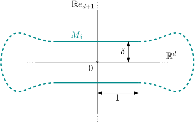
Figure 10: Diagram of a candidate for $M_{\delta}$.

We endow each $M_{\delta}$ with a density $f_{\delta}$ such that

$$\forall z\in O(\delta),~{}~{}f_{\delta}(z)=f_{\max}~{}~{}~{}\text{and}~{}~{}~{}\forall z\in O(-\delta),~{}~{}f_{\delta}(z)=f_{\min}$$

and we denote $Q_{\delta}=f_{\delta}d\mu_{M_{\delta}}$. If $f_{\min}$ is small enough (due to the constraint $\operatorname{vol}\operatorname{supp}P\leq 1/f_{\min}$ for any $P\in\Sigma^{d}_{\alpha,\beta}$) we can always choose $M_{\delta}$ and $f_{\delta}$ so that $\|\iota_{M_{\delta}}\|_{\mathcal{H}^{\alpha+1}}\leq R/2$ and $\|f_{\delta}\|_{\mathcal{H}^{\beta}}\leq L/2$.

Let now $\Phi:\mathbb{R}^{d+1}\to\mathbb{R}$ be a smooth, positive, radial function with support in $B(0,1)$ with $\Phi(0)=1$. Because the exponential map smoothly depends on the metric, for any $h<1$, there exists $\delta_{h}\in(0,h)$ sufficiently small such that the push-forward measures of $Q_{\delta_{h}}$ through the mappings

$$\Psi^{+}_{h}(z)=\operatorname{Id}-\delta_{h}\Phi\left(\frac{z-\delta_{h}e_{d+1}}{h}\right)e_{d+1}~{}~{}~{}~{}\text{and}~{}~{}~{}~{}\Psi^{-}_{h}(z)=\operatorname{Id}+\delta_{h}\Phi\left(\frac{z+\delta_{h}e_{d+1}}{h}\right)e_{d+1}$$

are both in $\Sigma^{d}_{\alpha,\beta}$. We write $N_{h}^{\pm}=\Psi^{\pm}_{h}(M_{\delta_{h}})$, $P_{h}^{\pm}=\left(\Psi^{\pm}_{h}\right)_{*}(Q_{\delta_{h}})$ and $g_{h}^{\pm}$ for the continuous version of the density $dP_{h}^{\pm}/d\mu_{N_{h}^{\pm}}$. See Figure 11 for a diagram of $N_{h}^{+}$ and $N_{h}^{-}$.

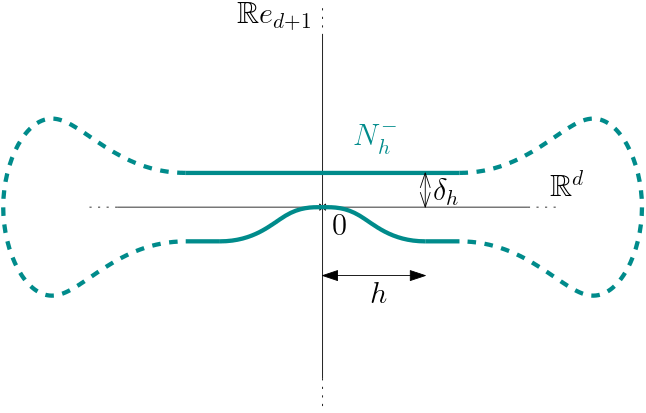
Figure 11: Diagram of manifolds $N_{h}^{+}$ (Left) and $N_{h}^{-}$ (right).

Using Lemma A.4, we obtain

$$\inf_{\widehat{f}}\sup_{P\in\Sigma^{d}_{\alpha,\beta}}\mathbb{E}_{P^{\otimes n}}[|\widehat{f}(0)-f_{P}(0)|^{p}]^{1/p}\geq\frac{1}{2}|g_{h}^{+}(0)-g_{h}^{-}(0)|\left(1-n\operatorname{TV}\left(P_{h}^{+},P_{h}^{-}\right)\right).$$

But now $g_{h}^{+}(0)=f_{\delta_{h}}(\delta_{h}e_{d+1})\times|\det d\Psi_{h}^{+}(\delta_{h}e_{d+1})|^{-1}=f_{\max}$ and, likewise, $g_{h}^{-}(0)=f_{\min}$. As for the total variation distance, we get

$$\operatorname{TV}\left(P_{h}^{+},P_{h}^{-}\right) =P_{h}^{+}(\Psi_{h}^{+}(hO(\delta_{h}))+P_{h}^{+}(hO(-\delta_{h}))+P_{h}^{-}(\Psi_{h}^{-}(hO(-\delta_{h}))+P_{h}^{-}(hO(\delta_{h}))$$

$$=2\operatorname{vol}(hO(\delta_{h}))\times\left(f_{\min}+f_{\max}\right)=2\zeta_{d}h^{d}\left(f_{\min}+f_{\max}\right)$$

where we recall that $\zeta_{d}$ is the volume of the $d$-dimensional unit-ball. Putting all the estimates together, we conclude

$$\inf_{\widehat{f}}\sup_{P\in\Sigma^{d}_{\alpha,\beta}}\mathbb{E}_{P^{\otimes n}}[|\widehat{f}(0)-f_{P}(0)|^{p}]^{1/p}\geq\frac{1}{2}(f_{\max}-f_{\min})\left(1-2n\zeta_{d}h^{d}\left(f_{\min}+f_{\max}\right)\right).$$

Letting $h$ goes to $0$ yields the result. ∎

A.3 Proof of Theorem 3.2

Proof of Theorem 3.2.

Suppose without loss of generality that $x=0$ and consider a smooth submanifold $M$ of $\mathbb{R}^{d+1}\subset\mathbb{R}^{D}$ that contains the disk $B_{\mathbb{R}^{d}}(0,1)\subset\mathbb{R}^{d}\times\{0_{\mathbb{R}^{D-d}}\}$ with reach greater than $\tau$, see Figure 12 for a diagram of such an $M$. By smoothness and compacity of $M$, there exists $L_{*}$ (depending on $\tau$) such that $M\in\mathcal{C}_{d,\alpha}(\tau,L_{*})$. Let $P$ be the uniform probability measure over $M$, with density $f:x\mapsto 1/\operatorname{vol}M$. We have $P\in\Sigma^{d}_{\alpha,\beta}$ as long as $L^{*}\leq L$ and $f_{\min}\leq 1/\operatorname{vol}M\leq f_{\max}$ an assumption we make from now on. For $0<\delta\leq 1$, let $P_{\delta}=f_{\delta}\cdot d\mu_{M}$ with

$$f_{\delta}(y)=\begin{cases}f(y)+\delta^{\beta}G(y/\delta)~{}~{}~{}\text{if}~{}~{}y\in B(0,\delta)\\ f(y)~{}~{}~{}\text{otherwise}\end{cases}$$

with $G:\mathbb{R}^{d}\rightarrow\mathbb{R}$ a smooth function with support in $B_{\mathbb{R}^{d}}(0,1)$ and such that $\int_{\mathbb{R}^{d}}G(y)dy=0$. We pick $G$ such that $f_{\delta}\in\mathcal{F}_{\beta}$ for small enough $\delta$, depending on $\tau$. Such a $G$ can be chosen to depend on $R$ only.

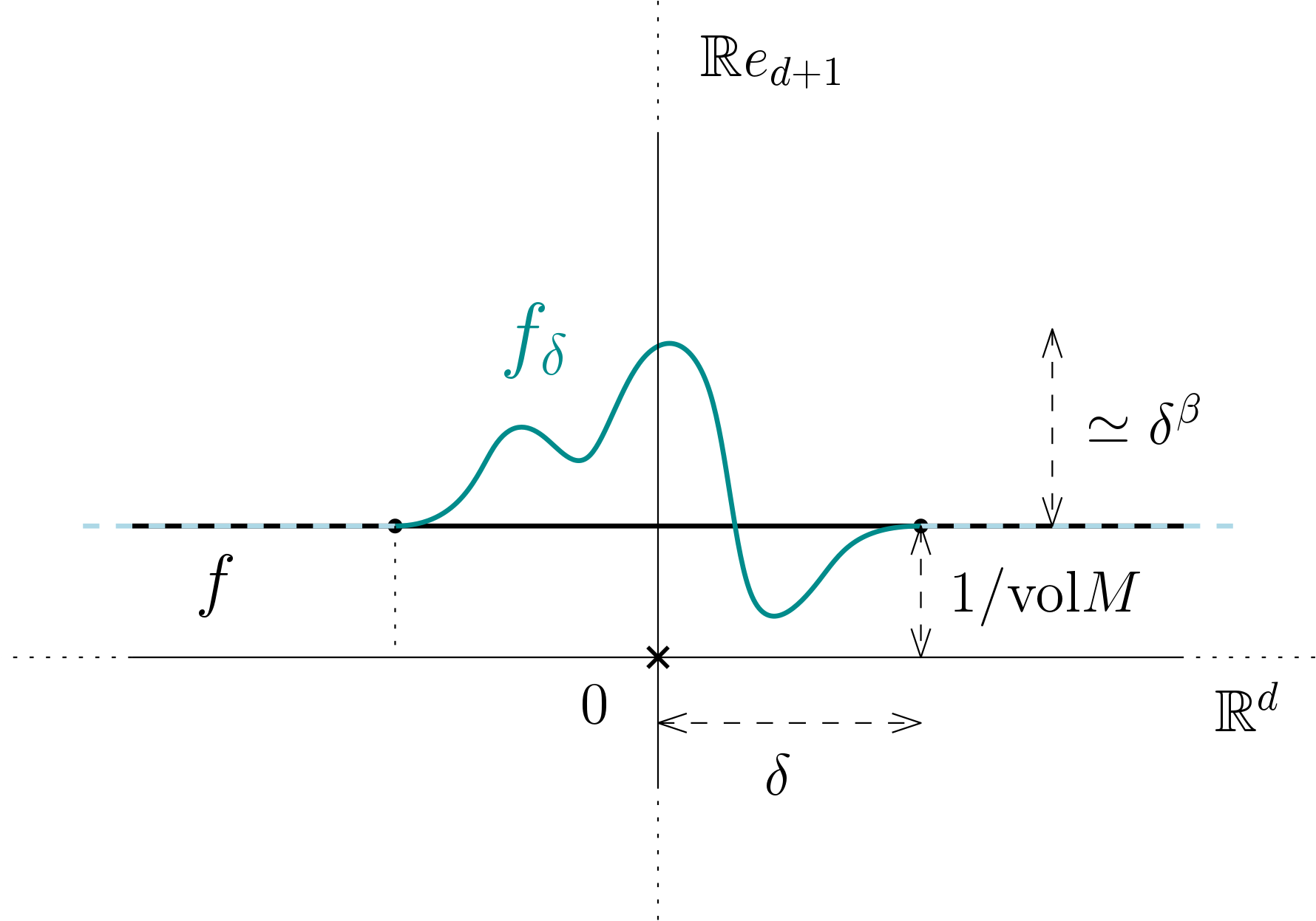
Figure 12: Diagram of a candidate for $M$ (Left) and of the densities $f$ and $f_{\delta}$ around $0$ (Right).

For $\delta$ small enough (depending on $\tau$), we thus have $P_{\delta}\in\Sigma^{d}_{\alpha,\beta}$ as well. By Lemma A.4, we infer

$$\inf_{\widehat{f}}\sup_{P\in\Sigma^{d}_{\alpha,\beta}}\mathbb{E}_{P^{\otimes n}}[|\widehat{f}(x)-f_{P}(x)|^{p}]^{1/p}\geq\tfrac{1}{2}\delta^{\beta}|G(0)|\left(1-\sqrt{2-2(1-H^{2}(P,P_{\delta}))^{n}}\right)$$

so that it remains to compute $H^{2}(P,P_{\delta})$. We have the following bound

$$H^{2}(P,P_{\delta}) =\int_{B_{\mathbb{R}^{d}}(0,\delta)}(1-\sqrt{1+\operatorname{vol}M\delta^{\beta}G(z/\delta)})^{2}dz$$

$$\leq\int_{B_{\mathbb{R}^{d}}(0,\delta)}(\operatorname{vol}M)^{2}\delta^{2\beta}G^{2}(z/\delta)dz$$

$$\leq(C\vee 1)\delta^{2\beta+d}$$

with $C=\operatorname{vol}M\times\int_{B(0,1)}G(z)^{2}dz$ depending on $\tau$ and $R$ only. Taking $\delta=(1/(C\vee 1)n)^{1/(2\beta+d)}$ we obtain, for large enough $n$ (depending on $\tau$)

$$\inf_{\widehat{f}}\sup_{P\in\Sigma^{d}_{\alpha,\beta}}\mathbb{E}_{P^{\otimes n}}[|\widehat{f}(x)-f_{P}(x)|^{p}]^{1/p}\geq\tfrac{1}{2}\big{(}(C\vee 1)n\big{)}^{-\beta/(2\beta+d)}\sqrt{2-2(1-1/n)^{n}}\geq C_{*}n^{-\beta/(2\beta+d)},$$

with $C_{*}=(C\vee 1)^{-1/2}$ depending on $\tau$ and $R$. ∎

A.4 Proofs of Section 3.2

We set $K_{h}(z)=h^{-d}K(z/h)$ and start with bounding the variance of $K_{h}(X-x)$ when $X$ is distributed according to $P\in\Sigma^{d}_{\alpha,\beta}$. Let first observe that

$$|K_{h}(X-x)|\leq\frac{\|K\|_{\infty}}{h^{d}}\mathbbm{1}_{B_{D}(x,h)}(X)\leq\frac{\|K\|_{\infty}}{h^{d}}$$ (20)

Lemma A.5.

For any $P\in\Sigma^{d}_{\alpha,\beta}$ and for any $h\leq\tau/2$,

$$\operatorname{Var}_{P}(K_{h}(X-x))\leq\frac{\omega}{h^{d}}~{}~{}~{}\text{where}~{}~{}\omega=4^{d}\zeta_{d}\|K\|_{\infty}^{2}b.$$

with $\zeta_{d}$ being the volume of the unit ball in $\mathbb{R}^{d}$.

Proof.

We have

$$\operatorname{Var}_{P}(K_{h}(X-x))\leq\mathbb{E}_{P}[K_{h}(X-x)^{2}]\leq\frac{\|K\|_{\infty}^{2}}{h^{2d}}P(B(x,h))\leq\frac{4^{d}\zeta_{d}f_{\max}\|K\|_{\infty}^{2}}{h^{d}}$$

where we used (20) and Lemma A.3 with $\eta=\tau/2$. ∎

Using Bernstein inequality (Boucheron et al., 2013, Thm. 2.10 p.37), for any $P\in\Sigma^{d}_{\alpha,\beta}$ and any $t>0$, we infer

$$\mathbb{P}\left(\big{|}\widehat{\xi}_{h}(P,x)\big{|}\geq\sqrt{\frac{2\omega t}{nh^{d}}}+\frac{\|K\|_{\infty}t}{nh^{d}}\right)\leq 2e^{-t},$$ (21)

where $\mathbb{P}$ is a short-hand notation for the distribution $P^{\otimes n}$ of the $n$-sample $X_{1},\ldots,X_{n}$ taken under $P$. The bound (21) is the main ingredient needed to bound the $L_{p}$-norm of the stochastic deviation of $\widehat{f}_{h}$.

Proof of Proposition 3.5.

We denote by $u_{+}=\max\{u,0\}$ the positive part of a real number $u$. We start with

$$\mathbb{E}_{P^{\otimes n}}\big{[}|\widehat{\xi}_{h}(P,x)|^{p}\big{]}\leq 2^{p-1}\left(\Omega(h)^{p}+\mathbb{E}_{P^{\otimes n}}\big{[}\big{(}|\widehat{\xi}_{h}(P,x)|-\Omega(h)\big{)}^{p}_{+}\big{]}\right).$$

The first term has the right order. For the second one, we make use of (21) to infer

$$\mathbb{E}_{P^{\otimes n}}\big{[}\big{(}|\widehat{\xi}_{h}(P,x)|-\Omega(h)\big{)}^{p}_{+}\big{]} =\int_{0}^{\infty}\mathbb{P}\left(|\widehat{\xi}_{h}(P,x)|>\Omega(h)+u\right)pu^{p-1}du$$

$$=p\Omega(h)^{p}\int_{0}^{\infty}\mathbb{P}\left(|\widehat{\xi}_{h}(P,x)|>\Omega(h)(1+u)\right)u^{p-1}du$$

$$\leq p\Omega(h)^{p}\left(1+\int_{1}^{\infty}\mathbb{P}\left(|\widehat{\xi}_{h}(P,x)|>\sqrt{\frac{2\omega(1+u)}{nh^{d}}}+\frac{\|K\|_{\infty}(1+u)}{nh^{d}}\right)u^{p-1}du\right)$$

$$\leq p\Omega(h)^{p}\left(1+\int_{1}^{\infty}2e^{-1-u}u^{p-1}du\right)$$

$$\leq p\Omega(h)^{p}(1+\Gamma(p))$$

which ends the proof. ∎

The proof of Lemma 3.7 partly relies on the following elementary lemma.

Lemma A.6.

Let $\gamma\geq 0$ be a real number and let $g:\mathbb{R}^{m}\rightarrow\mathbb{R}$ for $m\in\mathbb{N}^{*}$ satisfying that $\|g\|_{\infty}\leq b$ and that the restriction of $g$ to $B(0,r)$ (denoting here the open ball in $\mathbb{R}^{m}$) is $\beta$-Hölder, meaning that

$$\forall v,w\in B(0,r),~{}~{}~{}~{}\|d^{k}g(v)-d^{k}g(w)\|\leq A\|v-w\|^{\delta}$$

for some $A>0$ with $k=\lceil\gamma-1\rceil$ and $\delta=\gamma-k$. Then there exists a constant $C$ (depending on $m,\gamma,r,b$ and $A$, and depending on $m$ and $\gamma$ when $r=\infty$) such that, for all $1\leq j\leq k$,

$$\sup_{v\in B(0,r/2)}\|d^{j}g(v)\|_{\operatorname{op}}\leq Cb^{1-j/\gamma}A^{j/\gamma}.$$

Proof.

Let $v\in B(0,r/2)$. Since $g$ is $\gamma$-Hölder on $B(0,r)$, we know that there exists a function $R_{v}$ such that, for any $z$ such that $v+z\in B(0,r)$, we have

$$g(v+z)-\sum_{j=0}^{k}\frac{1}{j!}d^{j}g(v)[z^{\otimes k}]=R_{v}(z)$$

with $|R_{v}(z)|\leq A\|z\|^{\beta}/k!$. Let $h=(2b{k}!/A)^{1/\gamma}$, and $z_{0}\in\mathbb{R}^{m}$ be unit-norm. Pick $a_{1},\dots,a_{k}\in(0,1)$ all distincts and small enough such that $ha_{k}z_{0}\in B(0,r/2)$ for all $k$ (if $r=\infty$, then we can pick the $a_{i}$ independently from $A$, $b$ and $\gamma$). Introducing the vectors of $\mathbb{R}^{k}$

$$X =\left(hdg(v)[z_{0}],\dots,\frac{h^{k}}{k!}d^{k}g(v)[z^{\otimes k}_{0}]\right)~{}~{}~{}~{}\text{and}$$

$$Y =\left(g(v+ha_{1}z_{0})-g(v)-R_{v}(ha_{1}z_{0}),\dots,g(v+ha_{k}z_{0})-g(v)-R_{v}(ha_{k}z_{0})\right)$$

we have $Y=VX$ with $V$ being the Vandermonde matrix associated with the real numbers $(a_{1},\dots,a_{k})$. The former being invertible, we have $\|X\|\leq\|V^{-1}\|_{\operatorname{op}}\|Y\|$ and thus, for any $1\leq j\leq k$

$$\left|\frac{h^{j}}{j!}d^{j}g(v)[z_{0}^{\otimes k}]\right|\leq\|V^{-1}\|_{\operatorname{op}}\left(2b+\frac{A}{k!}h^{\gamma}\right).$$

Substituing the value of $h$ and noticing that the former inequality holds for every unit-norm vector $z_{0}$, we can conclude.

∎

Proof of Lemma 3.7.

We set $B_{h}=B(x,h)$. Since $\tau/2$ is smaller than the injectivity radius of $\exp_{x}$ (see Proposition 2.3) we can write

$$f_{h}(P,x)=\int_{B_{h}}K_{h}\left(p-x\right)f(p)d\mu_{M}(p)=\int_{\exp_{x}^{-1}B_{h}}K_{h}(\exp_{x}v-x)f(\exp_{x}v)\zeta(v)dv$$ (22)

with $\zeta(v)=\sqrt{\det g^{x}(v)}$. We set $\gamma=\alpha\wedge\beta$ and $k=\lceil\gamma-1\rceil$. Let $F$ denote the map $f\circ\exp_{x}$. For $h$ smaller than $\tau/2$, we have $\exp_{x}^{-1}B_{h}\subset B_{T_{x}M}(0,2h)\subset B_{T_{x}M}(0,\tau)$ (see Proposition A.2). We can thus write the following expansion, valid for all $v\in\exp_{x}^{-1}B_{h}$ and all $w\in T_{x}M$,

$$\exp_{x}(v)=x+v+\sum_{j=2}^{k+1}\frac{1}{j!}d^{j}\exp_{x}(0)[v^{\otimes j}]+R_{1}(v)~{}~{}~{} \text{with}~{}~{}\|R_{1}(v)\|\leq C_{1}\|v\|^{\gamma+1},$$ (23)

$$F(v)=f(x)+\sum_{j=1}^{k}\frac{1}{j!}d^{j}F(0)[v^{\otimes j}]+R_{2}(v)~{}~{}~{} \text{with}~{}~{}|R_{2}(v)|\leq C_{2}\|v\|^{\gamma},$$ (24)

$$K(v+w)=\mathbbm{1}_{\{\|v+w\|\leq 1\}}\left(K(v)+\sum_{j=1}^{k}\frac{1}{j!}d^{j}K(v)[w^{\otimes j}]+R_{3}(v,w)\right)~{}~{}~{} \text{with}~{}~{}|R_{3}(v,w)|\leq C_{3}\|w\|^{\gamma},$$ (25)

with $C_{1}$ depending on $\alpha,\tau$ and $L$, $C_{2}$ depending on $\beta,\tau,f_{\max}$ and $R$ (see Lemma A.6), and $C_{3}$ depending on $K$. Since now we know that $g^{x}_{ij}(v)=\langle d\exp_{x}(v)[e_{i}],d\exp_{x}(v)[e_{j}]\rangle$, we have a similar expansion for the mapping $\zeta(v)=\sqrt{\det g^{x}(v)}$

$$\zeta(v)=1+\sum_{j=1}^{k}\frac{1}{j!}d^{j}\zeta(0)[v^{\otimes j}]+R_{4}(v)~{}~{}~{} \text{with}~{}~{}|R_{4}(v)|\leq C_{4}\|v\|^{\gamma}$$ (26)

with $C_{4}$ depending on $\alpha,\tau$ and $L$. Making the change of variable $v=hw$ in (22), we get

$$f_{h}(P,x)=\sum_{k=0}^{k}G_{j}(h,P,x)+R_{h}(P,x)$$

with $G_{j}$ corresponding to the integration of the $j$-th order terms in the expansion around $0$ of the function $v\mapsto K\left(\frac{p-\exp_{p}(hw)}{h}\right)F(hw)\zeta(hw)$. In particular $G_{j}$ can be written as a sum of terms of the type

$$I=h^{j}\int_{\frac{1}{h}\exp_{x}^{-1}B_{h}}d^{m}K(w)[\phi(w)^{\otimes m}]\psi(w)dw$$

where $\psi$ and $\phi$ are monomials in $w$ satisfying $m\deg\phi+\deg\psi=j$, with coefficients bounded by constants depending on $\alpha,\tau,L,\beta,f_{\max}$ and $R$ (again, use Lemma A.6 to bound the derivatives). Since now $B_{T_{x}M}(0,1)\subset\frac{1}{h}\exp_{x}^{-1}B_{h}$, and since $d^{j}K$ is zero outside of $B(0,1)$, we have that $G_{j}$ can actually be written $G_{j}(h,P,x)=h^{j}G_{j}(P,x)$ with $|G_{j}(P,x)|\leq C$ for some $C$ depending on $K,\alpha,\tau,L,\beta,f_{\max}$ and $R$. Similar reasoning leads to $R_{h}(P,x)\leq Ch^{\gamma}$ with $C$ depending again on $K,\alpha,\tau,L,\beta,f_{\max}$ and $R$. To conclude, it remains to compute $G_{0}(P,x)$. Looking at the zero-th order terms in the expansions (23) to (26), we find that

$$G_{0}(P,x)=\int_{B_{T_{x}M}(0,1)}K(w)f(x)dw=f(x)$$

where we used Assumption 3.6. The proof of Lemma 3.7 is complete. ∎

Proof of Proposition 3.8.

For a positive integer $\ell\geq 1$, let $f_{h}^{(\ell)}(P,x)$ be the mean of the estimator $\widehat{f}_{h}(x)$ computed using $K^{(\ell)}$. Let $\gamma=\alpha\wedge\beta$ and $k=\lceil\gamma-1\rceil$. We recursively prove on $1\leq\ell<\infty$ the following identity

$$\forall h\leq\tau/2,~{}~{}~{}f^{(\ell)}_{h}(P,x)=f(x)+\sum_{j=\ell}^{k}h^{j}G^{(\ell)}_{j}(P,x)+R^{(\ell)}_{h}(P,x)$$ (27)

where $|R^{(\ell)}_{h}(P,x)|\leq C^{(\ell)}h^{\gamma}$ for some constant $C^{(\ell)}$ depending on $\tau,\ell,L,R,f_{\max}$ and $\beta$. The initialisation step $\ell=1$ has been proven in Lemma 3.7. Let now $1\leq\ell\leq k$. By linearity of $f_{h}(P,x)$ with respect to $K$, we have

$$f^{(\ell+1)}_{h}(P,x)=2f^{(\ell)}_{2^{-1/\ell}h}(P,x)-f^{(\ell)}_{h}(P,x).$$

Since $2^{-1/\ell}h\leq h$, we can use our induction hypothesis (27) and find

$$f^{(\ell+1)}_{h}(P,x)=f(x)+\sum_{j=\ell}^{k}(2^{1-j/\ell}-1)h^{j}G^{(\ell)}_{j}(P,x)+2R^{(\ell)}_{2^{-1/\ell}h}(P,x)-R^{(\ell)}_{h}(P,x).$$

We conclude noticing that $2^{1-j/\ell}-1=0$ for $j=\ell$, and setting $G^{(\ell+1)}_{j}(P,x)=(2^{1-j/\ell}-1)G^{(\ell)}_{j}(P,x)$ and $R^{(\ell+1)}_{h}(P,x)=2R^{(\ell)}_{2^{-1/\ell}h}(P,x)-R^{(\ell)}_{h}(P,x)$. The new remainder term verifies

$$|R^{(\ell+1)}_{h}(P,x)|\leq(2^{1-\gamma/\ell}+1)C^{(\ell)}h^{\gamma}\leq 3C^{(\ell)}h^{\gamma}$$ (28)

ending the induction by setting $C^{(\ell+1)}=3C^{(\ell)}$. When $\ell\geq k+1$, the induction step is trivial. ∎

A.5 Proofs of Section 3.3

Proof of Lemma 3.9.

Let $\gamma:[0,L_{M}]\rightarrow M$ be a unit speed parametrization of $M$ and extend $\gamma$ to a smooth function on $\mathbb{R}$ by $L_{M}$-periodicity. Suppose without loss of generality that $\gamma(0)=z$. For any $t\in\mathbb{R}$, there is a canonical identification between $T_{\gamma(t)}M$ and $\mathbb{R}$ through the map $v\mapsto\langle\dot{\gamma}(t),v\rangle$. With such an identification, we can write that for $s\in\mathbb{R}\simeq T_{z}M$, $\exp_{z}(s)=\gamma(s)$ because $\gamma$ is unit-speed. We thus have $d\exp_{z}(s)[h]=h\dot{\gamma}(s)$ for any $h\in T_{\gamma(s)}M\simeq\mathbb{R}$. It follows that $\det g^{z}(s)=\|d\exp_{z}(s)[1]\|^{2}=\|\dot{\gamma}(s)\|^{2}=1$ and this completes the proof. ∎

We write $V=\left(x,X_{1},\dots,X_{n}\right)$ for the vertices of $\mathcal{G}_{\varepsilon}$ and $\widehat{\eta}=\sup_{z\in M}d(z,V)$. For small enough $\widehat{\eta}$ we have that $\mathcal{G}_{\varepsilon}$ is connected, therefore the distance $\widehat{d}_{\varepsilon}$ is well-defined on $V$. We have in that case a good reverse control of $d_{M}$ by $\widehat{d}_{\varepsilon}$, as shown in the next two lemmata.

Lemma A.7.

If $\varepsilon\leq 8\tau$ and $16\widehat{\eta}\leq\varepsilon$, then $\widehat{d}_{\varepsilon}(y,z)\leq d_{M}(y,z)$ for any $y,z\in V$.

Lemma A.8.

If $\varepsilon\leq\tau/2$, then $d_{M}(y,z)\leq\left(1+\frac{\pi^{2}}{48\tau^{2}}\varepsilon^{2}\right)\widehat{d}_{\varepsilon}(p,q)$ for any $y,z\in V$.

Proof of Lemma A.7.

We can take the shortest path in $M$ between $y$ and $z$ as a unit-speed path of the form $\gamma:[0,\ell]\rightarrow\mathbb{R}^{D}$ with $\ell=d_{M}(y,z)\leq L_{M}/2$. We let $\delta=\ell/(4\lfloor\ell/\varepsilon\rfloor)$ and $N=4\lfloor\ell/\varepsilon\rfloor$. Notice that $\varepsilon/4\leq\delta\leq\varepsilon/2$. Let us define $p_{j}=\gamma(j\delta)$, so that $p_{0}=y$ and $p_{N}=z$. Since $\widehat{\eta}\leq\varepsilon/16$, for every $1\leq j\leq N-1$, there exists among our vertices $V$ a point denoted by $\widehat{p}_{j}$ such that $\|p_{j}-\widehat{p}_{j}\|\leq\varepsilon/16$. We set $\widehat{t}_{j}\in[0,L_{M}]$ for its coordinate, namely $\widehat{p}_{j}=\gamma(\widehat{t}_{j})$.

Let us show first that for $1\leq j<N$, we have $\widehat{t}_{j}\in[0,\ell]$. Indeed, thanks to Proposition A.2, since $\varepsilon/16\leq\tau/2$, we have $|t_{j}-\widehat{t}_{j}|\leq 2\|p_{j}-\widehat{p}_{j}\|\leq\varepsilon/8$. Since $\delta\geq\varepsilon/4$, we thus have $0\leq\widehat{t}_{1}\leq\dots\leq\widehat{t}_{N-1}\leq\ell$. Furthermore, writing $\widehat{p}_{0}=y$ and $\widehat{p}_{N}=z$, we have

$$\|\widehat{p}_{j}-\widehat{p}_{j+1}\|\leq\|\widehat{p}_{j}-p_{j}\|+\|p_{j}-p_{j+1}\|+\|p_{j+1}-\widehat{p}_{j+1}\|\leq\varepsilon$$

for any $0\leq j<\ell$. The sequence $s=(\widehat{p}_{0},\dots,\widehat{p}_{N})$ is thus a path in $\mathcal{G}_{\varepsilon}$ and so

$$\widehat{d}_{\varepsilon}(p,q)\leq L_{s}=\|\widehat{p}_{1}-\widehat{p}_{0}\|+\dots+\|\widehat{p}_{N}-\widehat{p}_{N-1}\|\leq|\widehat{t}_{1}-\widehat{t}_{0}|+\dots+|\widehat{t}_{N}-\widehat{t}_{N-1}|=\widehat{t}_{N}-\widehat{t}_{0}$$

where we set $\widehat{t}_{0}=0$ and $\widehat{t}_{N}=\ell=d_{M}(p,q)$, ending the proof. ∎

Proof of Lemma A.8.

Following the proof of (Arias-Castro and Le Gouic, 2019, Lem. 5) if there exists $\delta>0$ such that $\|y-z\|\leq\delta$ implies $d_{M}(y,z)\leq\pi\tau$ for all $y,z\in M$, then we must have that for any $y,z\in M$ satisfying $\|y-z\|\leq\delta$,

$$d_{M}(x,y)\leq\left(1+\frac{\pi^{2}}{48\tau^{2}}\|y-z\|^{2}\right)\|y-z\|.$$

Thanks to Proposition A.2, this must hold for $\delta=\tau/2$. Now let $p_{0},\dots,p_{m}$ be the shortest path in $\mathcal{G}_{\varepsilon}$ between $y$ and $z$. Since $\varepsilon\leq\tau/2$, we have

$$d_{M}(p,q) \leq\sum_{j=1}^{m}d_{M}(p_{j},p_{j-1})\leq\sum_{j=1}^{m}\left(1+\frac{\pi^{2}}{48\tau^{2}}\|p_{j}-p_{j-1}\|^{2}\right)\|p_{j}-p_{j-1}\|$$

$$\leq\left(1+\frac{\pi^{2}}{48\tau^{2}}\varepsilon^{2}\right)\widehat{d}_{\varepsilon}(p,q)$$

which ends the proof. ∎

In view of Lemma A.7 and Lemma A.8, we want to tune $\varepsilon$ so that it is the smallest possible and so that $16\widehat{\eta}\leq\varepsilon$ holds with high probability. This is achieved for $\varepsilon$ of order $\log n/n$.

Lemma A.9.

Setting $\varepsilon=\frac{32(p+1)\log n}{f_{\min}n}$, for every $n\geq 3$, we have $\mathbb{P}\left(16\widehat{\eta}\leq\varepsilon\right)\geq 1-1/n^{p}$.

Proof.

Let $\delta>0$, and let $N=\lfloor L_{M}/\delta\rfloor$. We split $[0,L_{M}]$ into $N$ intervals $I_{1},\dots,I_{N}$ of length $L_{M}/N$. We denote $\mathcal{A}$ the event for which each $I_{j}$ contains at least one coordinate among those of the sample of observations $(X_{1},\dots,X_{n})$. On $\mathcal{A}$, we have $\widehat{\eta}\leq L_{M}/N\leq 2\delta$. Moreover,

$$\mathbb{P}(\mathcal{A}) =1-\mathbb{P}\left(\exists j,~{}\gamma(I_{j})~{}\text{contains no observation}\right)$$

$$\geq 1-N\left(1-\min_{1\leq j\leq N}P(\gamma(I_{j}))\right)^{n}\geq 1-N\left(1-\frac{aL_{M}}{N}\right)^{n}.$$

Using that $N\leq L_{M}/\delta$ and that $L_{M}\leq 1/a$ we infer

$$\mathbb{P}\left(\widehat{\eta}\leq 2\delta\right)\geq 1-\frac{1}{a\delta}(1-a\delta)^{n}\geq 1-\frac{e^{-a\delta n}}{a\delta}.$$

Setting $\delta=\frac{(p+1)\log n}{an}$ and $\varepsilon=32\delta$ yields

$$\mathbb{P}\left(16\widehat{\eta}\leq\varepsilon\right)\geq 1-\frac{n}{(p+1)n^{p+1}\log n}\geq 1-\frac{1}{n^{p}}$$

as soon as $\log n\geq 1$, i.e. for $n\geq 3$. ∎

Proof of Proposition 3.10.

Recall that we set $K^{\operatorname{1D}}=K^{(1,\ell)}$ where $K^{(1,\ell)}$ is defined starting from kernel $\lambda_{1}^{-1}\Lambda$. Let $\mathcal{A}$ be the event $\{16\widehat{\eta}\leq\varepsilon\}$. By triangle inequality, $\mathbb{E}_{P^{\otimes n}}[|\hat{f}^{\operatorname{1D}}_{h}(x)-f_{P}(x)|^{p}]^{1/p}\leq\mathcal{R}_{\mathcal{A}}+\mathcal{R}_{\mathcal{A}^{c}}$, with

$$\mathcal{R}_{\mathcal{A}}=\left(\mathbb{E}_{P^{\otimes n}}\big{[}|\hat{f}^{\operatorname{1D}}_{h}(x)-f_{P}(x)|^{p}\mathbbm{1}_{\mathcal{A}}\big{]}\right)^{1/p}~{}~{}~{}\text{and}~{}~{}~{}\mathcal{R}_{\mathcal{A}^{c}}=\left(\mathbb{E}_{P^{\otimes n}}\big{[}|\hat{f}^{\operatorname{1D}}_{h}(x)-f_{P}(x)|^{p}\mathbbm{1}_{\mathcal{A}^{c}}\big{]}\right)^{1/p}.$$

On $\mathcal{A}$, we have, for $n$ large enough (depending on $p,f_{\min}$ and $\tau$) such that $\varepsilon\leq\tau/2$ holds, $|\widehat{d}_{\varepsilon}(X_{i},x)-d_{M}(X_{i},x)|\leq C_{1}\varepsilon^{2}$ with $C_{1}$ depending on $\tau$ only. This is infered by Lemmas A.7 and A.8. We deduce that, on this event,

$$\left|\hat{f}_{h}^{\operatorname{1D}}(x)-\hat{g}^{\operatorname{1D}}_{h}(x)\right|\leq\frac{C_{1}\|{K^{\operatorname{1D}}}^{\prime}\|_{\infty}\varepsilon^{2}}{h^{2}}~{}~{}~{}\text{with}~{}~{}~{}\hat{g}^{\operatorname{1D}}_{h}(x)=\frac{1}{n}\sum_{i=1}^{n}K^{\operatorname{1D}}_{h}(d_{M}(X_{i},x)).$$

It follows that

$$\mathcal{R}_{\mathcal{A}} \leq\frac{C_{1}\|{K^{\operatorname{1D}}}^{\prime}\|_{\infty}\varepsilon^{2}}{h^{2}}+\left(\mathbb{E}_{P^{\otimes n}}\big{[}|\hat{g}^{\operatorname{1D}}_{h}(x)-f_{P}(x)|^{p}\big{]}\right)^{1/p}$$

$$\leq\frac{C_{1}\|{K^{\operatorname{1D}}}^{\prime}\|_{\infty}\varepsilon^{2}}{h^{2}}+\left(\mathbb{E}_{P^{\otimes n}}\big{[}|\widehat{\xi}_{h}^{*}(P,x)|^{p}\big{]}\right)^{1/p}+|\mathcal{B}_{h}^{*}(P,x)|$$

with $\mathcal{B}_{h}^{*}$ and $\widehat{\xi}_{h}^{*}$ denoting the bias and stochastic deviation of estimator $\hat{g}^{\operatorname{1D}}_{h}(x)$. Following the same arguments as in proof of Proposition 3.5, we have $\mathbb{E}_{P^{\otimes n}}[|\widehat{\xi}_{h}^{*}(P,x)|^{p}]^{1/p}\leq c_{p}\Omega(h)^{p}$ with $c_{p}$ depending only on $p$. For the bias term, as soon as $h\leq\pi\tau$, we have

$$\mathcal{B}^{*}_{h}(P,x) =\mathbb{E}_{P^{\otimes n}}[\hat{g}^{\operatorname{1D}}_{h}(x)]-f(x)=\int_{M}K^{\operatorname{1D}}_{h}(d(p,x))f(p)d\mu_{M}(p)-f(x)$$

$$=\int_{B_{T_{x}M}(0,1)}K^{\operatorname{1D}}(\|v\|)\left(f\circ\exp_{x}(hv)-f(x)\right)dv.$$

Since now $f\circ\exp_{x}$ is $\beta$-Hölder on $B_{T_{x}M}(0,\pi\tau)$, we know that all the terms in the development of $\mathcal{B}_{h}^{*}(P,x)$ up to order $\lceil\beta-1\rceil$ cancels. We deduce $|\mathcal{B}_{h}^{*}(P,x)|\leq C_{2}h^{\beta}$ with $C_{2}$ depending on $\ell$ and $R$ only. For the other term $\mathcal{R}_{\mathcal{A}^{c}}$, we write $|\hat{f}^{\operatorname{1D}}_{h}(x)-f(x)|\leq\frac{\|K^{\operatorname{1D}}\|_{\infty}}{h}+f_{\max},$ so that, according to Lemma A.9,

$$\mathcal{R}_{\mathcal{A}^{c}}\leq\left(\frac{\|K^{\operatorname{1D}}\|_{\infty}}{h}+f_{\max}\right)\mathbb{P}(\mathcal{A}^{c})^{1/p}\leq C_{3}\frac{1}{nh}$$

with $C_{3}$ depending on $\ell$ and $f_{\max}$. Putting all these estimates together yields the result. ∎

A.6 Proofs of Section 3.4

Lemma A.10.

For any $P\in\Sigma^{d}_{\alpha,\beta}$, and $\Theta>p$, we have

$$\mathbb{E}_{P^{\otimes n}}[|\widehat{f}(x)-f_{P}(x)|^{p}]^{1/p}\lesssim\Omega(h^{*}(P,x))\lambda(h^{*}(P,x))$$

up to a constant depending on $p$ and $\Theta$, with

$$h^{*}(P,x)=\max\big{\{}h\in\mathbb{H}~{}|~{}\forall\eta\in\mathbb{H}(h),~{}|f_{\eta}(P,x)-f(x)|\leq\frac{1}{2}\Omega(h)\lambda(h)\big{\}}.$$

Proof.

We fix $P\in\Sigma^{d}_{\alpha,\beta}$ and write $\widehat{h}$ and $h^{*}$ for $\widehat{h}(x)$ and $h^{*}(P,x)$ respectively. Let $\mathcal{A}=\{\widehat{h}\geq h^{*}\}$. We can write $\mathbb{E}_{P^{\otimes n}}[|\widehat{f}(x)-f_{P}(x)|^{p}]=\mathcal{R}_{\mathcal{A}}+\mathcal{R}_{\mathcal{A}^{c}}$, where

$$\mathcal{R}_{\mathcal{A}}=\mathbb{E}_{P^{\otimes n}}[|\widehat{f}(x)-f_{P}(x)|^{p}\mathbbm{1}_{\mathcal{A}}]~{}~{}~{}\text{and}~{}~{}~{}\mathcal{R}_{\mathcal{A}^{c}}=\mathbb{E}_{P^{\otimes n}}[|\widehat{f}(x)-f_{P}(x)|^{p}\mathbbm{1}_{\mathcal{A}^{c}}].$$

We start with bounding $\mathcal{R}_{\mathcal{A}}$. Firstly,

$$\begin{split}\mathcal{R}_{\mathcal{A}}\leq 3^{p-1}\big{(}&\mathbb{E}_{P^{\otimes n}}[|\widehat{f}_{\widehat{h}}(x)-\widehat{f}_{h^{*}}(x)|^{p}\mathbbm{1}_{\mathcal{A}}]+\mathbb{E}_{P^{\otimes n}}[|\widehat{f}_{h^{*}}(x)-f_{h^{*}}(P,x)|^{p}\mathbbm{1}_{\mathcal{A}}]\\ &+\mathbb{E}_{P^{\otimes n}}[|f_{h^{*}}(P,x)-f_{P}(x)|^{p}\mathbbm{1}_{\mathcal{A}}]\big{)}.\end{split}$$

Next, by definition of $\widehat{h}$ and $\mathcal{A}$, we have

$$|\widehat{f}_{\widehat{h}}(x)-\widehat{f}_{h^{*}}(x)|\mathbbm{1}_{\mathcal{A}}\leq\psi(\widehat{h},h^{*})\mathbbm{1}_{\mathcal{A}}\leq 2\Omega(h^{*})\lambda(h^{*}).$$

By definition of $h^{*}$, we also have $|f_{h^{*}}(P,x)-f(x)|\leq\frac{1}{2}\Omega(h^{*})\lambda(h^{*})$. Finally, using Proposition 3.5

$$\mathbb{E}_{P^{\otimes n}}[|\widehat{f}_{h^{*}}(x)-f_{h^{*}}(P,x)|^{p}\mathbbm{1}_{\mathcal{A}}]\leq c_{p}\Omega(h^{*})^{p}\leq c_{p}(\Omega(h^{*})\lambda(h^{*}))^{p}$$

holds as well. Putting all three inequalities together yields

$$\mathcal{R}_{\mathcal{A}}\leq C_{\mathcal{A}}(\Omega(h^{*})\lambda(h^{*}))^{p}~{}~{}~{}\text{with}~{}~{}~{}C_{\mathcal{A}}=3^{p-1}\left(2^{p}+c_{p}+2^{-p}\right).$$

We now turn to $\mathcal{R}_{\mathcal{A}^{c}}$. Notice that for any $h\in\mathbb{H}(h^{*})$, we have

$$|f_{h}(P,x)-f(x)|\leq\frac{1}{2}\Omega(h^{*})\lambda(h^{*})\leq\frac{1}{2}\Omega(h)\lambda(h),$$

hence

$$|\widehat{f}_{h}(x)-f(x)|\leq\frac{1}{2}\Omega(h^{*})\lambda(h^{*})+|\widehat{\xi}_{h}(P,x)|.$$

We can thus write

$$\mathcal{R}_{\mathcal{A}^{c}}=\sum_{h\in\mathbb{H}(h^{*}/2)}\mathbb{E}_{P^{\otimes n}}[|\widehat{f}_{h}(x)-f(x)|^{p}\mathbbm{1}_{\{\widehat{h}=h\}}]\leq\sum_{h\in\mathbb{H}(h^{*}/2)}\mathbb{E}_{P^{\otimes n}}\big{[}\big{(}\frac{1}{2}\Omega(h^{*})\lambda(h^{*})+|\widehat{\xi}_{h}(P,x)|]\big{)}^{p}\mathbbm{1}_{\{\widehat{h}=h\}}\big{]}.$$

Now, for any $h\in\mathbb{H}(h^{*}/2)$, we have

$$\{\widehat{h}=h\} \subset\{\exists\eta\in\mathbb{H}(h),~{}|\widehat{f}_{2h}(x)-\widehat{f}_{\eta}(x)|>\psi(2h,\eta)\}$$

$$\subset\bigcup_{\eta\in\mathbb{H}(h)}\left\{\Omega(h^{*})\lambda(h^{*})+|\widehat{\xi}_{2h,\eta}(P,x)|>\psi(2h,\eta)\right\},$$

where $\widehat{\xi}_{2h,\eta}(P,x)=\widehat{\xi}_{2h}(P,x)-\widehat{\xi}_{\eta}(P,x)$, and where we used the triangle inequality and the definition of $h^{*}$. Now, we have $\Omega(h^{*})\lambda(h^{*})\leq\Omega(2h)\lambda(2h)$ since $2h\leq h^{*}$ and by definition of $\psi(2h,\eta)$, we infer

$$\{\widehat{h}=h\}\subset\bigcup_{\eta\in\mathcal{H}(h)}\left\{|\widehat{\xi}_{2h,\eta}(P,x)|>\Omega(\eta)\lambda(\eta)\right\}$$

so that

$$\mathbb{P}(\widehat{h}=h) \leq\sum_{\eta\in\mathbb{H}(h)}\mathbb{P}\left(|\widehat{\xi}_{2h,\eta}(P,x)|>\Omega(\eta)\lambda(\eta)\right)$$ (29)

$$\leq\sum_{\eta\in\mathbb{H}(h)}\mathbb{P}\left(|\widehat{\xi}_{2h,\eta}(P,x)|>\sqrt{\frac{8\omega\lambda(\eta)}{n\eta^{d}}}+\frac{2\|K\|_{\infty}\lambda(\eta)}{n\eta^{d}}\right)$$

$$\leq\sum_{\eta\in\mathbb{H}(h)}2\exp(-\lambda(\eta)^{2}).$$ (30)

For (29) we use the fact that $\lambda(\eta)\geq 1$ and Bernstein’s inequality on the random variable $\widehat{\xi}_{2h,\eta}(P,x)$ for (30). Noticing now that $\lambda(\eta)^{2}\geq d\Theta\log(1/\eta)$, we further obtain

$$\mathbb{P}(\widehat{h}=h) \leq 2h^{\Theta d}\times\sum_{j=0}^{\lfloor\log_{2}(1/h^{-})\rfloor}2^{-j\Theta d}\leq\frac{2}{1-2^{-\Theta d}}h^{\Theta d}.$$

For any $h\in\mathbb{H}(h^{*}/2)$, we thus get the following bound, using Cauchy-Schwarz inequality

$$\mathbb{E}_{P^{\otimes n}}\big{[}\big{(}\frac{1}{2}\Omega(h^{*})\lambda(h^{*}) +|\widehat{\xi}_{h}(P,x)|]\big{)}^{p}\mathbbm{1}_{\{\widehat{h}=h\}}\big{]}$$

$$\leq\mathbb{P}(\widehat{h}=h)^{1/2}E_{P^{\otimes n}}\big{[}\big{(}\frac{1}{2}\Omega(h^{*})\lambda(h^{*})+|\widehat{\xi}_{h}(P,x)|]\big{)}^{2p}\big{]}^{1/2}$$

$$\leq 2^{(2p-1)/2}\sqrt{\frac{2}{1-2^{-\Theta d}}}h^{\Theta d/2}\left(2^{-p}\Omega(h^{*})^{p}\lambda(h^{*})^{p}+c_{2p}^{1/2}\Omega(h)^{p}\right).$$ (31)

We plan to sum over $h\in\mathbb{H}(h^{*}/2)$ the RHS of (31). Notice first that

$$\sum_{h<h^{*}}h^{\Theta d/2}\leq(h^{*})^{\Theta d/2}(1-2^{-\Theta d/2})^{-1}.$$

Moreover, for any $h\geq h^{-}$, we have $\Omega(h)\leq 2\sqrt{2\omega/(nh^{d})}$ by definition of $h^{-}$. It follows that

$$\Omega(h^{*})\leq\Omega(h)\leq 2\Omega(h^{*})\left(\frac{h^{*}}{h}\right)^{d/2}.$$

for any $h\leq h^{*}$. This enables us to bound the following sum

$$\sum_{h\in\mathbb{H}(h^{*}/2)}h^{\Theta d/2}\Omega(h)^{p} \leq 2^{p}\Omega(h^{*})^{p}{h^{*}}^{pd/2}\sum_{h\in\mathbb{H}(h^{*}/2)}h^{\Theta d/2-pd/2}$$

$$\leq\frac{2^{p}}{1-2^{(p-\Theta)d/2}}\Omega(h^{*}){h^{*}}^{\Theta d/2}$$

where we used that $\Theta>p$. Putting all these estimates together, using that $h^{*}\leq 1$ and $\lambda(h^{*})\geq 1$, we eventually obtain

$$\mathcal{R}_{\mathcal{A}^{c}}\leq C_{\mathcal{A}^{c}}\Omega(h^{*})^{p}\lambda(h^{*})^{p}~{}~{}\text{with}~{}~{}C_{\mathcal{A}^{c}}=\frac{2^{p}}{\sqrt{1-2^{-\Theta d}}}\left(\frac{2^{-p}}{1-2^{-\Theta d/2}}+\frac{\sqrt{c_{2p}}2^{p}}{1-2^{(p-\Theta)d/2}}\right).$$

In conclusion $\mathbb{E}_{P^{\otimes n}}[|\widehat{f}(x)-f_{P}(x)|^{p}]^{1/p}\leq(C_{\mathcal{A}}+C_{\mathcal{A}^{c}})\Omega(h^{*})^{p}\lambda(h^{*})^{p}$ which completes the proof. ∎

Proof of Theorem 3.4..

Let $P\in\Sigma^{d}_{\alpha,\beta}$ and let $\bar{h}=(\rho\log n/n)^{1/(2\gamma+d)}$ with $\gamma=\alpha\wedge\beta$ and for some constant $\rho$ to be specified later. By Proposition 3.8 we know that for $n$ large enough (depending on $\rho,\alpha,\beta,d$) such that $\bar{h}\leq\tau/2$, we have $|f_{\eta}(P,x)-f(x)|\leq C_{1}\eta^{\gamma}$ for all $\eta\leq\bar{h}$ with $C_{1}$ depending on $K,\ell,\alpha,\tau,L,\beta,f_{\max}$ and $R$. Moreover, we also have

$$\frac{2^{-2}\Omega(\bar{h})^{2}\lambda(\bar{h})^{2}}{C_{1}^{2}\bar{h}^{2\gamma}}\geq\frac{d\Theta 2\omega\log(1/\bar{h})}{4C_{1}^{2}n\bar{h}^{2\gamma+d}}=\frac{d\Theta\omega(2\gamma+d)^{-1}}{2C_{1}^{2}\rho}\frac{\log n-\log\log n-\log\rho}{\log n}.$$

Thus, picking $\rho=d\Theta\omega(2\gamma+d)^{-1}/(2C_{1}^{2})$ yields $C_{1}\bar{h}^{\gamma}\leq\frac{1}{2}\Omega(\bar{h})\lambda(\bar{h})$ for $n$ large enough (depending on $\rho$), and therefore $\bar{h}\leq h^{*}(P,x)$. By Lemma A.10 this implies

$$\mathbb{E}_{P^{\otimes n}}[|\widehat{f}(x)-f_{P}(x)|^{p}]^{1/p}\leq C_{2}\Omega(\bar{h})\lambda(\bar{h})$$

where $C_{2}$ depends on $p$ and $\Theta$. But using that both $\bar{h}\geq h^{-}$ and $\lambda(\bar{h})^{2}=d\Theta\log(1/\bar{h})$ for $n$ large enough (depending on $\rho,d,K$ and $\Theta$), we also obtain

$$\Omega(\bar{h})^{2}\lambda(\bar{h})^{2}\leq\frac{8\omega d\Theta\log(1/\bar{h})}{n\bar{h}^{d}}=\frac{8\omega d\Theta(2\gamma+d)^{-1}}{\rho}\frac{\log n-\log\log n-\log\omega}{\log n}\bar{h}^{2\gamma}\leq 16C_{1}^{2}\bar{h}^{2\gamma}.$$

This last estimate yields

$$\mathbb{E}_{P^{\otimes n}}[|\widehat{f}(x)-f_{P}(x)|^{p}]^{1/p}\leq\left(4C_{1}C_{2}\rho^{\gamma/(2\gamma+d)}\right)\left(\frac{\log n}{n}\right)^{\gamma/(2\gamma+d)}$$

for $n$ large enough depending on $\rho,\alpha,\beta,d,K$ and $\Theta$, which completes the proof. ∎

A.7 Proofs of Section 3.5

Proof of Proposition 3.13.

By the triangle inequality, for any $P\in\Sigma^{d}_{\alpha,\beta}$, we write

$$\mathbb{E}_{P^{\otimes n}}\big{[}|\widehat{f}_{\widehat{h}}(\widehat{d};x)-f_{P}(x)|^{p}\big{]}^{1/p}\leq\Big{(}\mathbb{E}_{P^{\otimes n}}\left[\left|\widehat{f}_{\widehat{h}}(\widehat{d};x)-f(x)\right|^{p}\mathbbm{1}_{\{\widehat{d}=d\}}\right]\Big{)}^{1/p}+\Big{(}\mathbb{E}_{P^{\otimes n}}\left[\left|\widehat{f}_{\widehat{h}}(\widehat{x};\cdot)-f(x)\right|^{p}\mathbbm{1}_{\{\widehat{d}\neq d\}}\right]\Big{)}^{1/p}.$$

The first term in the right-hand side has the right order thanks to Theorem 3.4. For the second one, using that $|f(x)|\leq f_{\max}$ and

$$|f_{\widehat{h}}(\widehat{d},x)|\leq\sup_{1\leq d<D}\frac{\|K^{(\ell)}(d,\cdot)\|_{\infty}}{(h_{d}^{-})^{d}}\lesssim n$$

up to a constant that depend on $D,K$ and $\ell$, we infer

$$\Big{(}\mathbb{E}_{P}\left[\left|\widehat{f}_{\widehat{h}}(\widehat{d};x)-f(x)\right|^{p}\mathbbm{1}_{\widehat{d}\neq d}\right]\Big{)}^{1/p}\lesssim\mathbb{P}\left(\widehat{d}\neq d\right)^{1/p}\times n.$$

Finally, since $\widehat{d}$ satisfies Assumption 3.12, we have

$$\mathbb{E}_{P^{\otimes n}}\big{[}|\widehat{f}_{\widehat{h}}(\widehat{d};x)-f_{P}(x)|^{p}\big{]}^{1/p}\lesssim\left(\frac{\log n}{n}\right)^{\alpha\wedge\beta/(2\alpha\wedge\beta+d)}+n^{-1/2}$$

for $n$ large enough depending on $p,\Theta,K,\ell,\alpha,\tau,L,\beta,f_{\max},f_{\min}$ and $R$, so that the result indeed holds up to a constant depending on the same parameters and $D$. ∎

Proof of Proposition 3.15.

Let $P\in\Sigma^{d}_{\alpha,\beta}$ and $\eta>0$. Assume that $\widehat{P}_{\eta}>0$. We have

$$|\widehat{\delta}_{\eta}-d| \leq|\log_{2}\widehat{P}_{2\eta}-\log_{2}P_{2\eta}|+|\log_{2}\widehat{P}_{\eta}-\log_{2}P_{\eta}|+|\log_{2}P_{2\eta}-\log_{2}P_{\eta}-d|$$

$$\leq\frac{1}{\log 2}\left(\frac{|\widehat{P}_{2\eta}-P_{2\eta}|}{\widehat{P}_{2\eta}\wedge P_{2\eta}}+\frac{|\widehat{P}_{\eta}-P_{\eta}|}{\widehat{P}_{\eta}\wedge P_{\eta}}\right)+\left|\log_{2}\left(P_{2\eta}/(2^{d}P_{\eta})\right)\right|$$

We first consider the determinist term. For $\eta\leq\tau/2$, we have, writing $r_{\eta}=\xi(\eta/\tau)\eta$ and using Lemma A.3,

$$L_{2\eta}(1-\eta^{2}/6\tau^{2})(2\eta)^{2}\zeta_{d}\leq P_{2\eta}\leq U_{2\eta}(1+r_{2\eta}^{2}/\tau^{2})r_{2\eta}^{d}\zeta_{d}$$

and

$$L_{\eta}(1-\eta^{2}/6\tau^{2})\eta^{d}\zeta_{d}\leq P_{\eta}\leq U_{\eta}(1+r_{\eta}^{2}/\tau^{2})r_{\eta}^{d}\zeta_{d},$$

where $L_{\eta}=\inf_{M\cap B(x,\eta)}f$ and $U_{\eta}=\sup_{M\cap B(x,\eta)}f$. Using again Lemma A.3, we have that for $\eta\leq\tau/2$, $M\cap B(x,\eta)\subset\exp_{x}B_{T_{x}M}(0,2\eta)$, and, since $2\eta\leq\pi\tau/2$ and that $f\in\mathcal{F}_{\beta}$, we know, using Lemma A.6, that there exists $R_{1}>0$ (depending on $\beta,\tau,f_{\max}$ and $R$) such that $f(x)-R_{1}\eta\leq L_{\eta}\leq U_{\eta}\leq f(x)+R_{1}\eta$. If $\eta<\tau/4$, the same bounds apply for $2\eta$ and we thus obtain

$$(f(x)-R_{1}2\eta)(1-\eta^{2}/6\tau^{2})(2\eta)^{d}\zeta_{d}\leq P_{2\eta}\leq(f(x)+R_{1}2\eta)(1+r_{2\eta}^{2}/\tau^{2})r_{2\eta}^{d}\zeta_{d}$$

and

$$(f(x)-R_{1}\eta)(1-\eta^{2}/6\tau^{2})\eta^{d}\zeta_{d}\leq P_{\eta}\leq(f(x)+R_{1}\eta)(1+r_{\eta}^{2}/\tau^{2})r_{\eta}^{d}\zeta_{d}.$$ (32)

Using these two inequalities, and the fact that $r_{\eta}/\eta\rightarrow 1$ as $\eta\rightarrow 0$, we find that $|P_{2\eta}/(2^{d}P_{\eta})-1|\lesssim\eta$ up to a constant that depends on $R_{1},\tau$ and $f_{\min}$, for $\eta$ small enough (depending on $R_{1},\tau$ and $f_{\min}$ as well). For the other terms, a simple use of Hoeffding’s inequality yields for any $\eta,\varepsilon>0$,

$$\mathbb{P}\left(|\widehat{P}_{\eta}-P_{\eta}|>\varepsilon\right)\leq 2\exp(-2n\varepsilon^{2}).$$

On the event $\mathcal{A}_{\eta}=\{|\widehat{P}_{\eta}-P_{\eta}|\leq\varepsilon\}$, we have moreover $\widehat{P}_{\eta}\wedge P_{\eta}\geq P_{\eta}-\varepsilon$. Setting $\varepsilon=\eta^{d+1}$, and using (32), we see that $P_{\eta}-\varepsilon\gtrsim\eta^{d}$ for $\eta$ small enough (depending on $R_{1},\tau$ and $f_{\min}$). Thus, on the event $\mathcal{A}_{\eta}\cap\mathcal{A}_{2\eta}$, with probability at least $1-4\exp(-2n\eta^{2d+2})$, we derive

$$|\widehat{\delta}_{\eta}-d|\lesssim\eta+\frac{\varepsilon}{P_{\eta}-\varepsilon}+\frac{\varepsilon}{P_{2\eta}-\varepsilon}\lesssim\eta,$$ (33)

for $\eta$ small enough (depending on $R_{1},\tau$ and $f_{\min}$), up to a constant that depends on $R_{1},\tau$ and $f_{\min}$. Now setting $\eta=n^{-1/(2D+2)}$, we have $\widehat{d}=\widehat{\delta}_{\eta}=d$ on the event $\mathcal{A}_{\eta}\cap\mathcal{A}_{2\eta}$ as soon as $n$ is large enough so that the LHS of (33) is strictly smaller than $1/2$, ending the proof. ∎

References

- Aamari (2017) Aamari, E. (2017). Vitesses de convergence en inférence géométrique. Ph. D. thesis, Paris Saclay.
- Aamari et al. (2019) Aamari, E., J. Kim, F. Chazal, B. Michel, A. Rinaldo, and L. Wasserman (2019). Estimating the reach of a manifold. Electron. J. Stat. 13(1), 1359–1399.
- Aamari and Levrard (2019) Aamari, E. and C. Levrard (2019). Nonasymptotic rates for manifold, tangent space and curvature estimation. Ann. Statist. 47(1), 177–204.
- Alexander and Bishop (2006) Alexander, S. B. and R. L. Bishop (2006). Gauss equation and injectivity radii for subspaces in spaces of curvature bounded above. Geometriae Dedicata 117(1), 65–84.
- Arias-Castro and Le Gouic (2019) Arias-Castro, E. and T. Le Gouic (2019). Unconstrained and curvature-constrained shortest-path distances and their approximation. Discrete & Computational Geometry 62(1), 1–28.
- Balakrishnan et al. (2012) Balakrishnan, S., A. Rinaldo, D. Sheehy, A. Singh, and L. Wasserman (2012). Minimax rates for homology inference. In Artificial Intelligence and Statistics, pp. 64–72.
- Baldi et al. (2009) Baldi, P., G. Kerkyacharian, D. Marinucci, D. Picard, et al. (2009). Adaptive density estimation for directional data using needlets. The Annals of Statistics 37(6A), 3362–3395.
- Bernstein et al. (2000) Bernstein, M., V. De Silva, J. C. Langford, and J. B. Tenenbaum (2000). Graph approximations to geodesics on embedded manifolds. Technical report, Technical report, Department of Psychology, Stanford University.
- Berry and Sauer (2017) Berry, T. and T. Sauer (2017). Density estimation on manifolds with boundary. Computational Statistics & Data Analysis 107, 1–17.
- Besse (1978) Besse, A. (1978). Manifolds all of whose Geodesics are Closed, Volume 93. Springer Science & Business Media.
- Boucheron et al. (2013) Boucheron, S., G. Lugosi, and P. Massart (2013). Concentration inequalities: A nonasymptotic theory of independence. Oxford university press.
- Bowman (1984) Bowman, A. W. (1984). An alternative method of cross-validation for the smoothing of density estimates. Biometrika 71(2), 353–360.
- Castillo et al. (2014) Castillo, I., G. Kerkyacharian, and D. Picard (2014). Thomas Bayes’ walk on manifolds. Probability Theory and Related Fields 158(3-4), 665–710.
- Chiu (1991) Chiu, S.-T. (1991). Bandwidth selection for kernel density estimation. Ann. Statist. 19(4), 1883–1905.
- Cleanthous et al. (2018) Cleanthous, G., A. Georgiadis, G. Kerkyacharian, P. Petrushev, and D. Picard (2018). Kernel and wavelet density estimators on manifolds and more general metric spaces. arXiv preprint arXiv:1805.04682.
- Devroye and Györfi (1985) Devroye, L. and L. Györfi (1985). Nonparametric density estimation. Wiley Series in Probability and Mathematical Statistics: Tracts on Probability and Statistics. John Wiley & Sons, Inc., New York. The view.
- Dubins (1957) Dubins, L. E. (1957). On curves of minimal length with a constraint on average curvature, and with prescribed initial and terminal positions and tangents. American Journal of mathematics 79(3), 497–516.
- Eugeciouglu and Srinivasan (2000) Eugeciouglu, Ö. and A. Srinivasan (2000). Efficient nonparametric density estimation on the sphere with applications in fluid mechanics. SIAM Journal on Scientific Computing 22(1), 152–176.
- Evans and Gariepy (1992) Evans, L. C. and R. F. Gariepy (1992). Measure theory and fine properties of functions. Chapman and Hall/CRC.
- Farahmand et al. (2007) Farahmand, A. M., C. Szepesvári, and J.-Y. Audibert (2007). Manifold-adaptive dimension estimation. In Proceedings of the 24th international conference on Machine learning, pp. 265–272. ACM.
- Federer (1959) Federer, H. (1959). Curvature measures. Transactions of the American Mathematical Society 93(3), 418–491.
- Federer (1969) Federer, H. (1969). Geometric measure theory. Springer.
- Fefferman et al. (2016) Fefferman, C., S. Mitter, and H. Narayanan (2016). Testing the manifold hypothesis. Journal of the American Mathematical Society 29(4), 983–1049.
- Gaïffas and Lecué (2007) Gaïffas, S. and G. Lecué (2007). Optimal rates and adaptation in the single-index model using aggregation. Electron. J. Stat. 1, 538–573.
- Gallot et al. (2004) Gallot, S., D. Hulin, and J. Lafontaine (2004). Riemannian geometry, Volume 3. Springer.
- Genovese et al. (2012) Genovese, C., M. Perone-Pacifico, I. Verdinelli, and L. Wasserman (2012). Minimax manifold estimation. Journal of machine learning research 13(May), 1263–1291.
- Giné and Nickl (2016) Giné, E. and R. Nickl (2016). Mathematical foundations of infinite-dimensional statistical models, Volume 40. Cambridge University Press.
- Goldenshluger and Lepski (2008) Goldenshluger, A. and O. Lepski (2008). Universal pointwise selection rule in multivariate function estimation. Bernoulli 14(4), 1150–1190.
- Goldenshluger and Lepski (2011) Goldenshluger, A. and O. Lepski (2011). Bandwidth selection in kernel density estimation: oracle inequalities and adaptive minimax optimality. Ann. Statist. 39(3), 1608–1632.
- Goldenshluger and Lepski (2014) Goldenshluger, A. and O. Lepski (2014). On adaptive minimax density estimation on . Probab. Theory Related Fields 159(3-4), 479–543.
- Hall et al. (1987) Hall, P., G. Watson, and J. Cabrera (1987). Kernel density estimation with spherical data. Biometrika 74(4), 751–762.
- Hartman (1951) Hartman, P. (1951). On geodesic coordinates. American Journal of Mathematics 73(4), 949–954.
- Hendriks (1990) Hendriks, H. (1990). Nonparametric estimation of a probability density on a Riemannian manifold using Fourier expansions. The Annals of Statistics, 832–849.
- Henry et al. (2013) Henry, G. S., A. L. Muñoz, and D. A. Rodriguez (2013). Locally adaptative density estimation on Riemannian manifolds.
- Hoffmann and Lepski (2002) Hoffmann, M. and O. Lepski (2002). Random rates in anisotropic regression. Ann. Statist. 30(2), 325–396. With discussions and a rejoinder by the authors.
- Izeddin et al. (2012) Izeddin, I., J. Boulanger, V. Racine, C. Specht, A. Kechkar, D. Nair, A. Triller, D. Choquet, M. Dahan, and J. Sibarita (2012). Wavelet analysis for single molecule localization microscopy. Optics express 20(3), 2081–2095.
- Kerkyacharian et al. (2012) Kerkyacharian, G., R. Nickl, and D. Picard (2012). Concentration inequalities and confidence bands for needlet density estimators on compact homogeneous manifolds. Probability Theory and Related Fields 153(1-2), 363–404.
- Kerkyacharian et al. (2011) Kerkyacharian, G., T. M. Pham Ngoc, and D. Picard (2011). Localized spherical deconvolution. Ann. Statist. 39(2), 1042–1068.
- Kim et al. (2016) Kim, J., A. Rinaldo, and L. Wasserman (2016). Minimax rates for estimating the dimension of a manifold. arXiv preprint arXiv:1605.01011.
- Kim and Koo (2002) Kim, P. T. and J.-Y. Koo (2002). Optimal spherical deconvolution. J. Multivariate Anal. 80(1), 21–42.
- Kim et al. (2009) Kim, P. T., J.-Y. Koo, and Z.-M. Luo (2009). Weyl eigenvalue asymptotics and sharp adaptation on vector bundles. J. Multivariate Anal. 100(9), 1962–1978.
- Klein et al. (2014) Klein, T., S. Proppert, and M. Sauer (2014). Eight years of single-molecule localization microscopy. Histochemistry and cell biology 141(6), 561–575.
- Lee (2006) Lee, J. M. (2006). Riemannian manifolds: an introduction to curvature, Volume 176. Springer Science & Business Media.
- Lepski and Serdyukova (2014) Lepski, O. and N. Serdyukova (2014). Adaptive estimation under single-index constraint in a regression model. Ann. Statist. 42(1), 1–28.
- Lepski et al. (1997) Lepski, O. V., E. Mammen, V. G. Spokoiny, et al. (1997). Optimal spatial adaptation to inhomogeneous smoothness: an approach based on kernel estimates with variable bandwidth selectors. The Annals of Statistics 25(3), 929–947.
- Lepskii (1992) Lepskii, O. (1992). Asymptotically minimax adaptive estimation. i: Upper bounds. optimally adaptive estimates. Theory of Probability & Its Applications 36(4), 682–697.
- Lepskiĭ (1990) Lepskiĭ, O. V. (1990). A problem of adaptive estimation in Gaussian white noise. Teor. Veroyatnost. i Primenen. 35(3), 459–470.
- Low (1992) Low, M. G. (1992). Nonexistence of an adaptive estimator for the value of an unknown probability density. Ann. Statist. 20(1), 598–602.
- Nikol’skii (2012) Nikol’skii, S. M. (2012). Approximation of functions of several variables and imbedding theorems, Volume 205. Springer Science & Business Media.
- Niyogi et al. (2008) Niyogi, P., S. Smale, and S. Weinberger (2008). Finding the homology of submanifolds with high confidence from random samples. Discrete & Computational Geometry 39(1-3), 419–441.
- Ozakin and Gray (2009) Ozakin, A. and A. G. Gray (2009). Submanifold density estimation. In Advances in Neural Information Processing Systems, pp. 1375–1382.
- Parzen (1962) Parzen, E. (1962). On estimation of a probability density function and mode. Ann. Math. Statist. 33, 1065–1076.
- Pelletier (2005) Pelletier, B. (2005). Kernel density estimation on Riemannian manifolds. Statistics & probability letters 73(3), 297–304.
- Richardson (1911) Richardson, L. F. (1911). Ix. the approximate arithmetical solution by finite differences of physical problems involving differential equations, with an application to the stresses in a masonry dam. Philosophical Transactions of the Royal Society of London. Series A, Containing Papers of a Mathematical or Physical Character 210(459-470), 307–357.
- Rudemo (1982) Rudemo, M. (1982). Empirical choice of histograms and kernel density estimators. Scand. J. Statist. 9(2), 65–78.
- Silverman (1986) Silverman, B. W. (1986). Density estimation for statistics and data analysis. Monographs on Statistics and Applied Probability. Chapman & Hall, London.
- Silverman (1998) Silverman, B. W. (1998). Density estimation for statistics and data analysis. Routledge.
- Stone (1982) Stone, C. J. (1982). Optimal global rates of convergence for nonparametric regression. Ann. Statist. 10(4), 1040–1053.
- Tenenbaum et al. (2000) Tenenbaum, J. B., V. De Silva, and J. C. Langford (2000). A global geometric framework for nonlinear dimensionality reduction. science 290(5500), 2319–2323.
- Triebel (1987) Triebel, H. (1987). Characterizations of function spaces on a complete Riemannian manifold with bounded geometry. Mathematische Nachrichten 130(1), 321–346.
- Tsybakov (2008) Tsybakov, A. (2008). Introduction to Nonparametric Estimation. Springer Series in Statistics. Springer New York.
- Van der Vaart (2000) Van der Vaart, A. W. (2000). Asymptotic statistics, Volume 3. Cambridge university press.
- Watson and Williams (1956) Watson, G. S. and E. J. Williams (1956). On the construction of significance tests on the circle and the sphere. Biometrika 43, 344–352.
- Wu and Wu (2020) Wu, H.-T. and N. Wu (2020). Strong uniform consistency with rates for kernel density estimators with general kernels on manifolds. arXiv preprint arXiv:2007.06408.
- Yu (1997) Yu, B. (1997). Assouad, Fano, and Le Cam. In Festschrift for Lucien Le Cam, pp. 423–435. Springer.