Optimal Approximate Quantum Error Correction for Quantum Metrology

Abstract

For a generic set of Markovian noise models, the estimation precision of a parameter associated with the Hamiltonian is limited by the $1/\sqrt{t}$ scaling where $t$ is the total probing time, in which case the maximal possible quantum improvement in the asymptotic limit of large $t$ is restricted to a constant factor. However, situations arise where the constant factor improvement could be significant, yet no effective quantum strategies are known. Here we propose an optimal approximate quantum error correction (AQEC) strategy asymptotically saturating the precision lower bound in the most general adaptive parameter estimation scheme where arbitrary and frequent quantum controls are allowed. We also provide an efficient numerical algorithm finding the optimal code. Finally, we consider highly-biased noise and show that using the optimal AQEC strategy, strong noises are fully corrected, while the estimation precision depends only on the strength of weak noises in the limiting case.

Introduction.–

Quantum metrology is one of the most important state-of-the-art quantum technologies, studying the precision limit of parameter estimation in quantum systems giovannetti2006quantum ; giovannetti2011advances ; degen2017quantum ; braun2018quantum ; pezze2018quantum ; pirandola2018advances . The task involves preparing a suitable initial state of the system, allowing it to evolve under quantum controls for a specific time, performing a suitable measurement, and inferring the value of the unknown system parameter from the measurement outcome. To enhance the estimation precision, a variety of quantum strategies have been proposed, such as squeezing the initial state caves1981quantum ; wineland1992spin ; kitagawa1993squeezed ; huelga1997improvement ; ulam2001spin ; demkowicz2013fundamental , optimizing the probing time chaves2013noisy , monitoring the environment plenio2016sensing ; albarelli2017ultimate ; albarelli2019restoring , exploiting non-Markovian effects matsuzaki2011magnetic ; chin2012quantum ; smirne2016ultimate , optimizing the control Hamiltonian yuan2016sequential ; liu2017quantum ; xu2019transferable and quantum error correction kessler2014quantum ; arrad2014increasing ; dur2014improved ; ozeri2013heisenberg ; reiter2017dissipative ; lu2015robust ; sekatski2017quantum ; demkowicz2017adaptive ; zhou2018achieving ; layden2018spatial ; layden2019ancilla ; gorecki2019quantum .

Quantum mechanics places a fundamental limit on estimation precision, the Heisenberg limit (HL), where the estimation precision scales like $1/N$ for $N$ probes; or equivalently, $1/t$ for a total probing time $t$. In the noiseless case, the HL is achievable using the maximally entangled state among probes leibfried2004toward ; giovannetti2006quantum . In practice, decoherence plays an indispensible role. Under many typical noise models, the estimation precision will follow the standard quantum limit (SQL) with scaling $1/\sqrt{N}$ (or $1/\sqrt{t}$) fujiwara2008fibre ; escher2011general ; ji2008parameter ; demkowicz2012elusive ; demkowicz2014using ; kolodynski2013efficient ; sekatski2017quantum ; demkowicz2017adaptive ; zhou2018achieving , the same as the central limit theorem scaling using classical strategies. Nevertheless, the superiority of quantum strategies over classical strategies by a constant-factor improvement, as opposed to a scaling improvement, was proven in several cases ulam2001spin ; escher2011general ; demkowicz2014using . There were also situations where the HL is achievable using quantum strategies even in the presence of noise zhou2018achieving ; albarelli2019restoring .

Due to the difficulty in obtaining the exact precision limits for general noise models using different quantum strategies, several asymptotical lower bounds have been proposed fujiwara2008fibre ; ji2008parameter ; escher2011general ; demkowicz2012elusive ; kolodynski2013efficient ; demkowicz2014using ; sekatski2017quantum ; demkowicz2017adaptive ; zhou2018achieving ; czajkowski2019many . For example, the channel simulation method was used to prove the SQL lower bound for programmable channels ji2008parameter ; demkowicz2012elusive ; demkowicz2014using . A necessary and sufficient condition of achieving the HL under Markovian noise was established using the channel extension method sekatski2017quantum ; demkowicz2017adaptive ; zhou2018achieving . Although these bounds have been successful at showing the scaling limit of quantum strategies, only in several special cases, the saturability of these lower bounds was established, e.g. for dephasing and erasure noise demkowicz2014using and for teleportation-covariant channels as a special type of programmable channels pirandola2017ultimate ; laurenza2018channel . A saturability statement of the SQL lower bound under general noise models and an efficient algorithm solving the optimal strategy remain missing up to the present day.

We address both of these open questions in this work. Here we consider parameter estimation under general Markovian noise using the most general adaptive sequential strategy (see Fig. 1). We propose an approximate quantum error correction (AQEC) strategy saturating the SQL lower bound of precision (asymptotically) and an efficient numerical algorithm solving the optimal AQEC codes for different noises. The saturability of the precision lower bound we prove here not only answers an important question in quantum metrology theory, but also paves the way for identifying the optimal quantum strategies in future experiments.

Quantum error correction (QEC) nielsen2002quantum was first shown useful in quantum metrology in a typical scenario where the dephasing noise in a qubit probe is corrected by QEC, while the $X$ (the Pauli-X operator) signal remains intact kessler2014quantum ; arrad2014increasing ; dur2014improved ; ozeri2013heisenberg . Later on, the result was generalized to arbitrary Markovian noise demkowicz2017adaptive ; zhou2018achieving , stating that the HL is achievable using the sequential QEC strategy if and only if the HNLS condition is satisfied, i.e. the signal Hamiltonian is not in the Lindblad span—an operator subspace defined using Lindblad operators gorini1976completely ; lindblad1976generators ; breuer2002theory . In practice, however, HNLS is often violated and the estimation precision is limited by the SQL, for example, sensing any single-qubit signal under depolarizing noise. Standard QEC strategies would be useless in this case, as the signal will be completely eliminated if the noise is fully corrected. However, here we show that by performing the QEC in an approximate fashion, the highest possible precision limit is achievable, marking another triumph of the QEC strategy in quantum metrology.

In this Letter, we first review the SQL precision lower bound under Markovian noise using the sequential strategy when HNLS is violated. Then we describe our AQEC strategy consisting of both a two-dimensional AQEC code and an optimal recovery channel. This allows the original quantum channel to be reduced to an effective channel where a $Z$ (the Pauli-Z operator) signal was sensed under dephasing noise—a special case where the precision lower bound was known to be saturable ulam2001spin ; escher2011general ; demkowicz2014using . Finally, we optimize the achievable precision over all possible AQEC codes, which coincides with the precision lower bound, completing the proof.

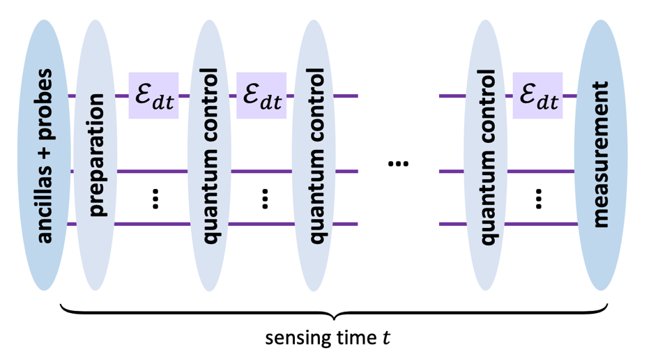
Figure 1: The most general adaptive sequential strategy where one probe sequentially senses the parameter for time $t$, with quantum controls (arbitrary completely positive and trace-preserving (CPTP) maps) applied every $dt$ and an arbitrary number of noiseless ancillas available. ${\mathcal{E}}_{dt}(\rho)=\rho+(-i[\omega H,\rho]+\sum_{i=1}^{r}L_{i}\rho L_{i}^{\dagger}-\frac{1}{2}\{L_{i}^{\dagger}L_{i},\rho\})dt+O(dt^{2})$ describes the evolution of the probe in an infinitesimally small time interval $dt$.

Precision lower bound.–

We assume the evolution of the quantum system is described by the following quantum master equation gorini1976completely ; lindblad1976generators ; breuer2002theory :

$$\frac{d\rho}{dt}=-i[\omega H,\rho]+\sum_{i=1}^{r}\Big{(}L_{i}\rho L_{i}^{\dagger}-\frac{1}{2}\{L_{i}^{\dagger}L_{i},\rho\}\Big{)},$$ (1)

where $\omega$ is the unknown parameter, $\rho\in{\mathcal{H}}_{S}\otimes{\mathcal{H}}_{A}$, ${\mathcal{H}}_{S}$ is the probe space $H$ and $\{L_{i}\}_{i=1}^{r}$ acting on ($H$, $L_{i}$ are shorthand for $H\otimes{\mathbbm{1}}$, $L_{i}\otimes{\mathbbm{1}}$, respectively) and ${\mathcal{H}}_{A}$ is the noiseless ancillary space (see Fig. 1). We assume $I,\{L_{i}\}_{i=1}^{r}$ are linearly independent, $\dim{\mathcal{H}}_{S}=d$ and $\dim{\mathcal{H}}_{A}=2d$. The Lindblad span associated with Eq. (1) is ${\mathcal{S}}={\rm span}\{{\mathbbm{1}},L_{i},L_{i}^{\dagger},L_{i}^{\dagger}L_{j},\forall i,j\}$, where ${\rm span}\{\cdot\}$ denotes the real linear subspace of Hermitian operators spanned by $\{\cdot\}$. According to the quantum Cramér-Rao bound helstrom1968minimum ; helstrom1976quantum ; braunstein1994statistical ; paris2009quantum , the standard deviation $\delta\omega$ of the $\omega$-estimator is bounded by $\delta\omega\geq(N_{\rm expr}F(t))^{-1/2}$, where $N_{\rm expr}$ is the number of experiments and $F(t)$ is the so-called quantum Fisher information (QFI) as a function of the final state $\rho(t)$. The bound is asymptotically saturable using the maximum likelihood estimator as $N_{\rm expr}$ goes to infinity casella2002statistical ; lehmann2006theory . Therefore, finding the optimal sequential strategy boils down to maximizing $F(t)$ over all input states and quantum controls. For an input state $\ket{\psi}$ evolving noiselessly under Hamiltonian $\omega H$, $F(t)=4t^{2}(\bra{\psi}H^{2}\ket{\psi}-(\bra{\psi}H\ket{\psi})^{2})$ and $\delta\omega\propto 1/t$ follows the HL. In the noisy case, it was proven that the HL is achievable if and only if $H\notin{\mathcal{S}}$ (the HNLS condition) and there exists a QEC strategy achieving the HL demkowicz2017adaptive ; zhou2018achieving .

The HNLS condition holds usually when the noise has a special structure, e.g. rank-one noise sekatski2017quantum or spacially correlated noise layden2018spatial ; layden2019ancilla . For generic noise, however, the HNLS condition is often violated. In this Letter, we focus on the latter situation where $H\in{\mathcal{S}}$ and the QFI follows the SQL demkowicz2017adaptive ; zhou2018achieving :

$$F(t)\leq 4t\min_{h,{\mathbf{h}},{\mathfrak{h}}|\beta=0}\left\|\alpha\right\|,$$ (2)

where $\left\|\cdot\right\|$ is the operator norm of a matrix, $h\in{\mathbb{R}}$, ${\mathbf{h}}\in{\mathbb{C}}^{r}$, ${\mathfrak{h}}\in{\mathbb{C}}^{r\times r}$ is hermitian,

$$\alpha =({\mathbf{h}}{\mathbbm{1}}+{\mathfrak{h}}{\mathbf{L}})^{\dagger}({\mathbf{h}}{\mathbbm{1}}+{\mathfrak{h}}{\mathbf{L}}),$$ (3)

$$\beta =H+h{\mathbbm{1}}+{\mathbf{h}}^{\dagger}{\mathbf{L}}+{\mathbf{L}}^{\dagger}{\mathbf{h}}+{\mathbf{L}}^{\dagger}{\mathfrak{h}}{\mathbf{L}},$$ (4)

where ${\mathbf{L}}:=(L_{1},L_{2},\ldots,L_{r})^{T}$ and ${\mathbf{h}}{\mathbbm{1}}:=({\mathbf{h}}_{1}{\mathbbm{1}},\ldots,{\mathbf{h}}_{r}{\mathbbm{1}})^{T}$. Here we introduce an AQEC strategy which (asymptotically) saturates the QFI upper bound up to an arbitrarily small error under arbitrary Markovian noise. That is, for any small $\delta>0$, there exists an AQEC strategy such that

$${\mathfrak{F}}:=\max_{t>0}\frac{F(t)}{t}=4\min_{h,{\mathbf{h}},{\mathfrak{h}}|\beta=0}\left\|\alpha\right\|-\delta,$$ (5)

where we define the normalized QFI ${\mathfrak{F}}$ as the objective function we maximize. The upper bound is saturated asymptotically in the sense that $\lim_{t\rightarrow\infty}F(t)/t={\mathfrak{F}}$.

Approximate quantum error correction.–

Here we propose a set of AQEC codes for quantum metrology and show that the effective channel under fast AQEC is an effective qubit dephasing channel in the logical space. In this way, identifying the optimal recovery channel for quantum metrology is equivalent to minimizing the noise rate of the dephasing channel where a closed-form solution exists, as opposed to generic AQEC scenarios where many known AQEC recovery channels are only suboptimal barnum2002reversing ; fletcher2007optimum ; beny2010general ; ng2010simple ; tyson2010two ; albert2018performance .

Let $P$ be the projection on to the code space $\ket{0_{\textsc{l}}}\bra{0_{\textsc{l}}}+\ket{1_{\textsc{l}}}\bra{1_{\textsc{l}}}$, where $\ket{0_{\textsc{l}}}$ and $\ket{1_{\textsc{l}}}$ are the logical zero and one states. Applying the AQEC quantum operation ${\mathcal{P}}+{\mathcal{R}}\circ{\mathcal{P}}_{\perp}$ infinitely fast, the effective evolution would be (up to the first order of $dt$ zhou2018achieving ; layden2019ancilla )

$$\frac{d\rho}{dt}=-i[\omega{\mathcal{P}}(H),\rho]+\sum_{i=1}^{r}\Big{(}{\mathcal{P}}(L_{i}\rho L_{i}^{\dagger})+\\ {\mathcal{R}}({\mathcal{P}}_{\perp}(L_{i}\rho L_{i}^{\dagger}))-\frac{1}{2}\{{\mathcal{P}}(L_{i}^{\dagger}L_{i}),\rho\}\Big{)},$$ (6)

where $P_{\perp}=1-P$, ${\mathcal{P}}(\cdot)=P(\cdot)P$, ${\mathcal{P}}_{\perp}(\cdot)=P_{\perp}(\cdot)P_{\perp}$ and ${\mathcal{R}}$ is a CPTP map describing the AQEC recovery channel. We define the following class of AQEC codes

$$\ket{0_{\textsc{l}}/1_{\textsc{l}}}=\sum_{ij}A_{0/1,ij}\ket{i}_{{\mathcal{H}}_{S}}\ket{j,0/1}_{{\mathcal{H}}_{A}},$$ (7)

where $A_{0},A_{1}\in{\mathbb{C}}^{d\times d}$ and $A_{0/1,ij}=C_{ij}\pm\varepsilon D_{ij}$ satisfy $\mathrm{Tr}(A_{0}A_{0}^{\dagger})=\mathrm{Tr}(A_{1}A_{1}^{\dagger})=1$ and $\mathrm{Tr}(C^{\dagger}D)=0$. Here $C$ describes the part of the code which $\ket{0_{\textsc{l}}}$ and $\ket{1_{\textsc{l}}}$ have in common and $D$ describes the part distinguishing $\ket{0_{\textsc{l}}}$ from $\ket{1_{\textsc{l}}}$ which generates non-zero signal and noise. In the special case where $\varepsilon=0$, the effective signal and noise are zero. Let ${\mathcal{H}}_{A}={\mathcal{H}}_{A^{\prime}}\otimes{\mathcal{H}}_{2}$ where $\dim{\mathcal{H}}_{A^{\prime}}=d$ and $\dim{\mathcal{H}}_{2}=2$, the last ancillary qubit in ${\mathcal{H}}_{2}$ makes the signal and noises both diagonal in the code space, i.e. $\braket{0_{\textsc{l}}}{H}{1_{\textsc{l}}}=\braket{0_{\textsc{l}}}{S}{1_{\textsc{l}}}=0$ for all $S\in{\mathcal{S}}$. Later on, we will assume $\varepsilon$ is a small parameter and consider the perturbation expansion of the effective dynamics around $\varepsilon=0$. We consider the recovery channel restricted to the structure (we will show that this type of recovery channels is sufficient for our purpose)

$${\mathcal{R}}(\cdot)=\sum_{m}\left(\ket{0_{\textsc{l}}}\bra{R_{m},0}+\ket{1_{\textsc{l}}}\bra{S_{m},1}\right)(\cdot)\\ \left(\ket{R_{m},0}\bra{0_{\textsc{l}}}+\ket{S_{m},1}\bra{1_{\textsc{l}}}\right),$$ (8)

where $\{\ket{R_{m}}\},\{\ket{S_{m}}\}\subset{\mathcal{H}}_{S}\otimes{\mathcal{H}}_{A^{\prime}}$ are two sets of orthonormal basis and ${\mathcal{R}}$ is CPTP. A few lines of calculation shows the effective channel (Eq. (6)) under the AQEC code (Eq. (7)) and the recovery channel (Eq. (8)) is

$$\frac{d\rho}{dt}\!=\!-\!i\left[\frac{\omega\mathrm{Tr}(HZ_{\textsc{l}})}{2}Z_{\textsc{l}}\!+\!H_{{\textsc{s}}},\rho\right]\!+\!\frac{\gamma({\mathcal{R}})}{2}\left(Z_{\textsc{l}}\rho Z_{\textsc{l}}\!-\!\rho\right),$$ (9)

where $Z_{\textsc{l}}=\ket{0_{\textsc{l}}}\bra{0_{\textsc{l}}}-\ket{1_{\textsc{l}}}\bra{1_{\textsc{l}}}$, $H_{{\textsc{s}}}$ is independent of $\omega$, and

$$\gamma({\mathcal{R}})=-{\mathrm{Re}}\Big{[}\sum_{i=1}^{r}\bra{0_{\textsc{l}}}\Big{(}{\mathcal{R}}({\mathcal{P}}_{\perp}(L_{i}\ket{0_{\textsc{l}}}\bra{1_{\textsc{l}}}L_{i}^{\dagger}))+\\ {\mathcal{P}}(L_{i}\ket{0_{\textsc{l}}}\bra{1_{\textsc{l}}}L_{i}^{\dagger})-\frac{1}{2}\{{\mathcal{P}}(L_{i}^{\dagger}L_{i}),\ket{0_{\textsc{l}}}\bra{1_{\textsc{l}}}\}\Big{)}\ket{1_{\textsc{l}}}\Big{]}.$$ (10)

We can remove the term $H_{{\textsc{s}}}$ in Eq. (9) by applying a reverse Hamiltonian constantly sekatski2017quantum . For dephasing channels, the optimal ${\mathfrak{F}}$ is reached using a special type of spin-squeezed state as the input kitagawa1993squeezed ; huelga1997improvement ; ulam2001spin ; escher2011general ; demkowicz2014using , where we have

$${\mathfrak{F}}=\frac{\mathrm{Tr}(HZ_{\textsc{l}})^{2}}{2\gamma({\mathcal{R}})}.$$ (11)

To simulate the evolution of multipartite spin-squeezed states using the sequential strategy where we have only a single probe, one could first prepare the desired spin-squeezed state in $\bigotimes_{i=1}^{N}{\mathcal{H}}_{i}$ by entangling the logical qubit in the effective dephasing channel (${\mathcal{H}}_{1}={\mathcal{H}}_{S}\otimes{\mathcal{H}}_{A}$) with a large number of ancillas ($\bigotimes_{i=2}^{N}{\mathcal{H}}_{i}$) where $\dim{\mathcal{H}}_{i}=\dim{\mathcal{H}}_{1}$ for $2\leq i\leq N$, and then perform swap operations between ${\mathcal{H}}_{1}$ and ${\mathcal{H}}_{i}$ for $i=2,\ldots,N$ successively every time $t/N$. The optimal ${\mathfrak{F}}$ in Eq. (11) is asymptotically attainable at $N\rightarrow\infty$ ulam2001spin .

For simplicity in furture calculation, we perform a two-step gauge transformation on the Lindblad operators $\{L_{i}\}_{i=1}^{r}$ to simplify the dynamics: (1) Let $L_{i}\leftarrow L_{i}-\mathrm{Tr}(C^{\dagger}L_{i}C)\cdot{\mathbbm{1}}$, such that $L_{i}$ satisfies $\mathrm{Tr}(C^{\dagger}L_{i}C)=0$ for all $L_{i}$. (2) Perform a unitary transformation $u\in{\mathbb{C}}^{r\times r}$ on the Lindblad operators ${\mathbf{L}}\leftarrow u{\mathbf{L}},$ such that $\mathrm{Tr}(C^{\dagger}L_{i}^{\dagger}L_{j}C)$ is a diagonal matrix. Note that above transformations only induce another parameter-independent shift $H_{\textsc{s}}$ in the Hamiltonian which could be eliminated by a reverse Hamiltonian. Now we have a new set of Lindblad operators $\{J_{i}\}_{i=1}^{r}$, satisfying

$$\mathrm{Tr}(C^{\dagger}J_{i}C)=0,\quad\mathrm{Tr}(C^{\dagger}J_{i}^{\dagger}J_{j}C)=\lambda_{i}\delta_{ij},$$ (12)

and we replace $\{L_{i}\}_{i=1}^{r}$ with $\{J_{i}\}_{i=1}^{r}$ in Eq. (10).

First, we maximize $\mathfrak{F}$ over the recovery ${\mathcal{R}}$, which is equivalent to minimizing $\gamma({\mathcal{R}})$ over ${\mathcal{R}}$. We claim that the minimum noise rate $\gamma=\min_{\mathcal{R}}\gamma({\mathcal{R}})$ is

$$\gamma=-\Big{\|}\sum_{i=1}^{r}{\mathcal{P}}_{\perp}(J_{i}\ket{0_{\textsc{l}}}\bra{1_{\textsc{l}}}J_{i}^{\dagger})\Big{\|}_{1}-{\mathrm{Re}}\Big{[}\sum_{i=1}^{r}\bra{0_{\textsc{l}}}\\ \Big{(}{\mathcal{P}}(J_{i}\ket{0_{\textsc{l}}}\bra{1_{\textsc{l}}}J_{i}^{\dagger})-\frac{1}{2}\{{\mathcal{P}}(J_{i}^{\dagger}J_{i}),\ket{0_{\textsc{l}}}\bra{1_{\textsc{l}}}\}\Big{)}\ket{1_{\textsc{l}}}\Big{]},$$ (13)

where we have used $\max_{U:U^{\dagger}U={\mathbbm{1}}}\mathrm{Tr}(MU+M^{\dagger}U^{\dagger})=2\left\|M\right\|_{1}$ for arbitrary square matrices $M$ and $U$, where $\left\|\cdot\right\|_{1}$ is the trace norm (see details in Appx. A of SM ).

Next, we could like to maximize ${\mathfrak{F}}$ over all possible AQEC codes of the form Eq. (7). It is not clear yet how that could be done mathematically with the presence of trace norm in the denominator. To arrive at an expression of $\gamma$ free of the trace norm, we further sacrifice the generality of our AQEC code and assume $\varepsilon\ll 1$. We call it the “perturbation” code in the sense that the signal and the noise are both infinitesimally small when $\varepsilon\rightarrow 0$. Under the limit $\varepsilon\rightarrow 0$, we have $\mathrm{Tr}(HZ_{\textsc{l}})=2\varepsilon\mathrm{Tr}(H\tilde{C})+O(\varepsilon^{2})$, where

$$\tilde{C}=CD^{\dagger}+DC^{\dagger},$$ (14)

and the noise rate is (ignoring all $o(\varepsilon^{2})$ terms)

$$\gamma=\varepsilon^{2}\bigg{(}\!\sum_{i}2\big{|}\mathrm{Tr}(J_{i}\tilde{C})\big{|}^{2}\!+\!\sum_{ij:\lambda_{i}+\lambda_{j}\neq 0}\!\frac{|\mathrm{Tr}(J_{i}^{\dagger}J_{j}\tilde{C})|^{2}}{(\lambda_{i}+\lambda_{j})}\!\bigg{)}.$$ (15)

For a detailed derivation of the noise rate, see Appx. B of SM and zhou2019an . Finally, we have the following expression of the normalized QFI (up to the lowest order of $\varepsilon$)

$${\mathfrak{F}}(C,\tilde{C})\!\approx\!\frac{\mathrm{Tr}(H\tilde{C})^{2}}{\sum_{i}\big{|}\mathrm{Tr}(J_{i}\tilde{C})\big{|}^{2}\!+\!\sum_{ij:\lambda_{i}+\lambda_{j}\neq 0}\!\frac{|\mathrm{Tr}(J_{i}^{\dagger}J_{j}\tilde{C})|^{2}}{2(\lambda_{i}+\lambda_{j})}},$$ (16)

as a function of $\tilde{C}$ and $C$ (implicitly through the choice of $\{J_{i}\}_{i=1}^{r}$). The effective dynamics of the perturbation code has the feature that both the signal and the noises are equally weak and only the ratio between them matters. Therefore the exact value of $\varepsilon$ will not influence the normalized QFI ${\mathfrak{F}}$ as long as it is sufficiently small. On the other hand, it does influence how fast $F(t)/t$ reaches its optimum ${\mathfrak{F}}$, characterized by a coherence time $O(1/\varepsilon^{2})$.

Saturating the bound.–

Now we maximize the normalized QFI (up to the lowest order of $\varepsilon$) over $C$ and $\tilde{C}$ and show that the optimal ${\mathfrak{F}}$ is exactly equal to its upper bound in Eq. (2). The domain of $C$ is all complex matrices satisfying $\mathrm{Tr}(C^{\dagger}C)=1$. We assume the domain of $\tilde{C}$ is all traceless Hermitian matrices satisfying $\mathrm{Tr}(J^{\dagger}_{i}J_{j}\tilde{C})=0$ for all $i,j\in{\mathfrak{n}}:=\{i|\lambda_{i}=0\}$. When $C$ is full-rank, ${\mathfrak{n}}$ is empty and for arbitrary traceless $\tilde{C}$, we could always take $D^{\dagger}=\frac{1}{2}C^{-1}\tilde{C}$ such that Eq. (14) is satisfied. When $C$ is singular, we could replace it with an approximate full-rank version (e.g. $C\leftarrow C+\delta{\mathbbm{1}}$). In this case, ${\mathfrak{F}}$ will only be decreased by an infinitesimal small amount when $\varepsilon=o(\delta^{2})$ because the numerator in Eq. (16) is only slightly perturbed after the replacement.

Consider the following optimization problem over $h,{\mathbf{h}},{\mathfrak{h}}$ and $C$,

$$\begin{split}&\max_{C}\min_{h,{\mathbf{h}},{\mathfrak{h}}}~{}~{}4\mathrm{Tr}(C^{\dagger}\alpha C),\\ &\;\text{subject~{}to~{}}~{}\beta=0,\quad\mathrm{Tr}(C^{\dagger}C)=1,\end{split}$$ (17)

Fixing $C$, we introduce a Hermitian matrix $\tilde{C}$ as the Lagrange multiplier associated with the constraint $\beta=0$ boyd2004convex . Strong duality implies Eq. (17) has the same solution as the following dual program (see Appx. C of SM )

$$\begin{split}\max_{C,\tilde{C}}~{}{\mathfrak{F}}(C,\tilde{C}),&\text{~{}~{}subject~{}to~{}}\mathrm{Tr}(C^{\dagger}C)=1,\,\mathrm{Tr}(\tilde{C})=0,\\ &~{}~{}\text{~{}and~{}}\mathrm{Tr}(J^{\dagger}_{i}J_{j}\tilde{C})=0,\forall i,j\in{\mathfrak{n}}.\end{split}$$ (18)

whose optimal value could be achieved using the perturbation code up to an infinitesimal small error according to the discussion above. On the other hand, thanks to Sion’s minimax theorem komiya1988elementary ; do2001introduction , we can exchange the order of the maximization and minimization in Eq. (17) because we could always confine $({\mathbf{h}},{\mathfrak{h}})$ in a convex and compact set (see Appx. D of SM ) such that the solution of Eq. (17) is not altered and the objective function $4\mathrm{Tr}(C^{\dagger}\alpha C)$ is concave (linear) with respect to $CC^{\dagger}$ and convex (quadratic) with respect to $({\mathbf{h}},{\mathfrak{h}})$. Therefore, the optimal value of Eq. (18) is also equal to $4\min_{h,{\mathbf{h}},{\mathfrak{h}}|\beta=0}\left\|\alpha\right\|$, the upper bound of the normalized QFI.

Numerical algorithm.–

It is known that the upper bound in Eq. (2) could be calculated via a semidefinite program (SDP) demkowicz2017adaptive ; czajkowski2019many ,

$$F(t)\leq 4t\min_{h,{\mathbf{h}},{\mathfrak{h}}|\beta=0}x,\text{~{}subject~{}to~{}}{\mathscr{A}}\succeq 0,\;\beta=0,$$ (19)

where ${\mathscr{A}}=\begin{pmatrix}\sqrt{x}{\mathbbm{1}}&{\mathbf{h}}^{\dagger}{\mathbbm{1}}+{\mathbf{L}}^{\dagger}{\mathfrak{h}}\\ {\mathbf{h}}{\mathbbm{1}}+{\mathfrak{h}}{\mathbf{L}}&\sqrt{x}{\mathbbm{1}}^{\otimes r}\\ \end{pmatrix}$ and “$\succeq 0$” means positive semidefinite. However, the minimax theorem does not guaranteed an efficient algorithm to solve Eq. (18) after exchanging the order of the maximization and minimization in Eq. (17). Now we provide an efficient numerical algorithm obtaining an optimal $(C^{\diamond},\tilde{C}^{\diamond})$ in three steps. The validity of this algorithm is proven in Appx. E of SM . The algorithm runs as follows: (a) Solving $\min_{h,{\mathbf{h}},{\mathfrak{h}}|\beta=0}\left\|\alpha\right\|$ using the SDP gives us an optimal $\alpha^{\diamond}$ (and corresponding $h^{\diamond},{\mathbf{h}}^{\diamond},{\mathfrak{h}}^{\diamond}$) satisfying $\left\|\alpha^{\diamond}\right\|=\min_{h,{\mathbf{h}},{\mathfrak{h}}|\beta=0}\left\|\alpha\right\|$. (b) Suppose $\Pi^{\diamond}$ is the projection onto the subspace spanned by all eigenstates corresponding to the largest eigenvalue of $\alpha^{\diamond}$, we find an optimal $C^{\diamond}C^{\diamond\dagger}$ satisfying $\Pi^{\diamond}C^{\diamond}C^{\diamond\dagger}\Pi^{\diamond}=C^{\diamond}C^{\diamond\dagger}$ and

$${\mathrm{Re}}[\mathrm{Tr}(C^{\diamond}C^{\diamond\dagger}({\Delta\mathbf{h}}{\mathbbm{1}}+{\Delta\mathfrak{h}}{\mathbf{L}})^{\dagger}({\mathbf{h}}^{\diamond}{\mathbbm{1}}+{\mathfrak{h}}^{\diamond}{\mathbf{L}}))]=0,$$ (20)

for all $({\Delta\mathbf{h}},{\Delta\mathfrak{h}})$ such that $\Delta h{\mathbbm{1}}+{\Delta\mathbf{h}}^{\dagger}{\mathbf{L}}+{\mathbf{L}}^{\dagger}{\Delta\mathbf{h}}+{\mathbf{L}}^{\dagger}{\Delta\mathfrak{h}}{\mathbf{L}}=0$ for some $\Delta h$. Note that this step is simply solving a system of linear equations. (c) Find $\{J_{i}\}_{i=1}^{r}$ via the gauge transformation. Let ${\mathcal{S}}_{0}={\rm span}\{I,J_{i}^{\dagger}J_{j},\forall i,j\in{\mathfrak{n}}\}$. Decompose $M=J_{i}$ or $J_{ij}$ ($:=J_{i}^{\dagger}J_{j}$) into $M=M^{h}+iM^{ah}+M_{0}^{h}+iM_{0}^{ah}$ where $M^{h,ah}$, $M_{0}^{h,ah}$ are Hermitian, $M_{0}^{h,ah}\in{\mathcal{S}}_{0}$ and $M^{h,ah}\perp{\mathcal{S}}_{0}$ (in terms of the Hilbert-Schmidt norm). Using the vectorization of matrices $|{\cdot}\rangle\!\rangle=\sum_{jk}\bra{j}(\cdot)\ket{k}\ket{j}\ket{k}$, let

$$B=\sum_{i}|{J_{i}^{h}}\rangle\!\rangle\langle\!\langle{J_{i}^{h}}|+|{J_{i}^{ah}}\rangle\!\rangle\langle\!\langle{J_{i}^{ah}}|+\\ \sum_{ij:\lambda_{i}+\lambda_{j}\neq 0}\frac{|{J_{ij}^{h}}\rangle\!\rangle\langle\!\langle{J_{ij}^{h}}|+|{J_{ij}^{ah}}\rangle\!\rangle\langle\!\langle{J_{ij}^{ah}}|}{2(\lambda_{i}+\lambda_{j})}.$$ (21)

According to the Cauchy-Schwarz inequality,

$$\max_{\tilde{C}}{\mathfrak{F}}(C^{\diamond},\tilde{C})=\max_{\tilde{C}}\frac{|\langle\!\langle{H|\tilde{C}}\rangle\!\rangle|^{2}}{\langle\!\langle{\tilde{C}|B|\tilde{C}}\rangle\!\rangle}=\langle\!\langle{H^{h}|B^{-1}|H^{h}}\rangle\!\rangle,$$ (22)

and the optimal $|{\tilde{C}^{\diamond}}\rangle\!\rangle=B^{-1}|{H^{h}}\rangle\!\rangle$. Here ^-1 means the Moore-Penrose pseudoinverse.

Highly-biased noise.–

We consider a special case where noises are separated into two groups – strong ones and weak ones zhou2018achieving ; layden2018spatial ; layden2019ancilla . To be specific, we consider the following quantum master equation

$$\frac{d\rho}{dt}=-i[\omega H,\rho]+\sum_{i\in{\bar{\mathfrak{s}}}}\eta\Big{(}L_{i}\rho L_{i}^{\dagger}-\frac{1}{2}\{L_{i}^{\dagger}L_{i},\rho\}\Big{)}\\ +\sum_{i\in{\mathfrak{s}}}\Big{(}L_{i}\rho L_{i}^{\dagger}-\frac{1}{2}\{L_{i}^{\dagger}L_{i},\rho\}\Big{)},$$ (23)

where the indices of Lindblad operators $\{L_{i}\}_{i=1}^{r}$ are separated into ${\bar{\mathfrak{s}}}$ and ${\mathfrak{s}}$, representing weak and strong noises respectively. $\eta\ll 1$ is a small parameter characterizing the relative strength of the weak noises. Moreover, we assume that $H\notin{\rm span}\{{\mathbbm{1}},L_{i},L_{i}^{\dagger},L_{i}^{\dagger}L_{j},\,i,j\in{\mathfrak{s}}\}$ so that it is possible to fully correct all strong noises and also preserve a non-trivial signal in the code space. Taking $\eta\rightarrow 0$, it is easy to show that (see Appx. F of SM ), the optimal ${\mathfrak{F}}$ in this case is equal to

$${\mathfrak{F}}^{\diamond}=\frac{1}{\eta}\left\|\bar{\alpha}\right\|_{h,{\mathbf{h}},{\mathfrak{h}}|\beta=0}+O(1),$$ (24)

where $\bar{\alpha}=({\mathbf{h}}{\mathbbm{1}}+{\mathfrak{h}}{\mathbf{L}})^{\dagger}\Pi_{\bar{\mathfrak{s}}}({\mathbf{h}}{\mathbbm{1}}+{\mathfrak{h}}{\mathbf{L}})$ and $\Pi_{\bar{\mathfrak{s}}}$ is a diagonal matrix whose $i$-th diagonal element is one when $i\in{\bar{\mathfrak{s}}}$ and zero when $i\in{\mathfrak{s}}$. This reduces the running time of the SDP in Eq. (19) by reducing ${\mathscr{A}}$ from a $d(r+1)\times d(r+1)$ matrix to a $d(\left|{\bar{\mathfrak{s}}}\right|+1)\times d(\left|{\bar{\mathfrak{s}}}\right|+1)$ matrix. Using the optimal AQEC strategy, ${\mathfrak{F}}$ is boosted by a factor of $O(1/\eta)$, compared to the case where no QEC is performed. To find the optimal AQEC code, we can solve the dual program of a modified version of Eq. (17) where $\alpha$ is replaced with $\bar{\alpha}$:

$$\max_{C,\tilde{C}}~{}\overline{{\mathfrak{F}}}(C,\tilde{C}), \text{~{}~{}subject~{}to~{}}\mathrm{Tr}(C^{\dagger}C)=1,\,\mathrm{Tr}(\tilde{C})=0,$$ (25)

$$~{}~{}\forall_{i,j\in{\mathfrak{s}}},\;\mathrm{Tr}(L^{\dagger}_{i}L_{j}\tilde{C})=\mathrm{Tr}(L_{i}\tilde{C})=0,$$ (26)

and some other linear contraints on $\tilde{C}$ when $\mathrm{Tr}(C{\mathbf{L}}^{\dagger}{\mathbf{L}}C)-\mathrm{Tr}(C{\mathbf{L}}^{\dagger}C)\mathrm{Tr}(C{\mathbf{L}}C)$ is singular. Here $\overline{{\mathfrak{F}}}$ is the dominant part of ${\mathfrak{F}}$ such that ${\mathfrak{F}}=\overline{{\mathfrak{F}}}/\eta+O(1)$. Detailed calculations including the expression of $\overline{{\mathfrak{F}}}$ and the dual program are provided in Appx. F of SM . The constraint Eq. (26) on $\tilde{C}$ is equivalent to the Knill-Laflamme condition for Lindblad operators $\{L_{i}\}_{i\in{\mathfrak{s}}}$ knill1997theory ; beny2011perturbative . It implies strong noises are fully corrected by the optimal AQEC code and explains why the estimation precision depends only on the strength of weak noises in Eq. (24).

Conclusions and outlook.–

In this Letter, we proposed an AQEC strategy such that the optimal SQL in Hamiltonian parameter estimation could be achieved asymptotically. An interesting open question is whether the perturbation code we introduced here could be turned into non-pertubative ones. We provide an example in Appx. G of SM , where by slightly modifying the ancilla-free QEC code (non-perturbation) proposed in Ref. layden2019ancilla , we show that the optimal ${\mathfrak{F}}$ could be achieved in the correlated dephasing noise model. However, it is unclear how to generalize the result to generic noise models. Another two interesting open questions are (1) how to characterize the power of QEC in improving quantum metroloy for parameters encoded in generic quantum channels demkowicz2012elusive ; demkowicz2014using , for example when the rate of quantum controls is constant, rather than infinitely fast; (2) how to optimize the QEC strategy when considering a constant probing time, rather than an infinitely long probing time.

Appendix A Minimizing the noise rate $\gamma({\mathcal{R}})$ over recovery channels ${\mathcal{R}}$

In this appendix we prove Eq. (13) in the main text. According to Eq. (10),

$$\gamma({\mathcal{R}})=-{\mathrm{Re}}\Big{[}\sum_{i=1}^{r}\bra{0_{\textsc{l}}}\Big{(}{\mathcal{R}}({\mathcal{P}}_{\perp}(J_{i}\ket{0_{\textsc{l}}}\bra{1_{\textsc{l}}}J_{i}^{\dagger}))+{\mathcal{P}}(J_{i}\ket{0_{\textsc{l}}}\bra{1_{\textsc{l}}}J_{i}^{\dagger})-\frac{1}{2}\{{\mathcal{P}}(J_{i}^{\dagger}J_{i}),\ket{0_{\textsc{l}}}\bra{1_{\textsc{l}}}\}\Big{)}\ket{1_{\textsc{l}}}\Big{]}.$$ (27)

In order to calculate $\gamma=\min_{\mathcal{R}}\gamma({\mathcal{R}})$, we only need to calculate the first term minimized over ${\mathcal{R}}$:

$$\begin{split}&\quad-\max_{\mathcal{R}}{\mathrm{Re}}\bigg{[}\sum_{i}\bra{0_{\textsc{l}}}{\mathcal{R}}({\mathcal{P}}_{\perp}(J_{i}\ket{0_{\textsc{l}}}\bra{1_{\textsc{l}}}J_{i}^{\dagger}))\ket{1_{\textsc{l}}}\bigg{]}\\ &=-\max_{\ket{R_{m}},\ket{S_{m}}}{\mathrm{Re}}\bigg{[}\sum_{i,m}\bra{R_{m},0}P_{\perp}J_{i}\ket{0_{\textsc{l}}}\bra{1_{\textsc{l}}}J_{i}^{\dagger}P_{\perp}\ket{S_{m},1}\bigg{]}\\ &=-\frac{1}{2}\max_{\ket{R_{m}},\ket{S_{m}}}\mathrm{Tr}\Big{(}\sum_{m}\ket{R_{m}}\bra{S_{m}}\cdot\sum_{i}\bra{0}P_{\perp}J_{i}\ket{0_{\textsc{l}}}\bra{1_{\textsc{l}}}J_{i}^{\dagger}P_{\perp}\ket{1}+h.c.\Big{)}\\ &=-\Big{\|}\sum_{i}\bra{0}P_{\perp}J_{i}\ket{0_{\textsc{l}}}\bra{1_{\textsc{l}}}J_{i}^{\dagger}P_{\perp}\ket{1}\Big{\|}_{1}=-\Big{\|}\sum_{i}P_{\perp}J_{i}\ket{0_{\textsc{l}}}\bra{1_{\textsc{l}}}J_{i}^{\dagger}P_{\perp}\Big{\|}_{1},\\ \end{split}$$ (28)

where $h.c.$ means Hermitian conjugate and we have used $\max_{U:U^{\dagger}U={\mathbbm{1}}}\mathrm{Tr}(MU+M^{\dagger}U^{\dagger})=2\left\|M\right\|_{1}$ for arbitrary square matrices $M$ and $U$, which could be proven easily using the singular value decomposition of $M$.

Appendix B Perturbation expansion of the noise rate $\gamma$

In this appendix we expand the minimum noise rate $\gamma$ around $\varepsilon=0$ using the perturbation code. For simplicity, the equal sign “$=$” in this appendix means approximate equality up to the second order of $\varepsilon$ (ignoring all $o(\varepsilon^{2})$ terms). We also state a useful lemma here:

Lemma 1 (mirsky1960symmetric ).

$\left\|X+\varepsilon Y\right\|_{1}=\left\|X\right\|_{1}+O(\varepsilon)$ for arbitrary $X$ and $Y$.

To calculate Eq. (13), we first consider the terms independent of ${\mathcal{R}}$,

$$\begin{split}&\quad-{\mathrm{Re}}\left[\sum_{i=1}^{r}\bra{0_{\textsc{l}}}\left({\mathcal{P}}(J_{i}\ket{0_{\textsc{l}}}\bra{1_{\textsc{l}}}J_{i}^{\dagger})-\frac{1}{2}\{{\mathcal{P}}(J_{i}^{\dagger}J_{i}),\ket{0_{\textsc{l}}}\bra{1_{\textsc{l}}}\}\right)\ket{1_{\textsc{l}}}\right]\\ &=-\sum_{i}{\mathrm{Re}}\big{[}\mathrm{Tr}(A_{0}A_{0}^{\dagger}J_{i})\mathrm{Tr}(A_{1}A_{1}^{\dagger}J_{i}^{\dagger})]-\frac{1}{2}\left(\mathrm{Tr}(A_{0}A_{0}^{\dagger}J_{i}^{\dagger}J_{i})+\mathrm{Tr}(A_{1}A_{1}^{\dagger}J_{i}^{\dagger}J_{i})\right)\\ &=\sum_{i}\lambda_{i}+\varepsilon^{2}\big{|}\mathrm{Tr}(\tilde{C}J_{i})\big{|}^{2}+\varepsilon^{2}\mathrm{Tr}(DD^{\dagger}J_{i}^{\dagger}J_{i}).\end{split}$$ (29)

The remaining term is equal to (thanks to Lemma 1) minus

$$\Big{\|}\sum_{i}P_{\perp}J_{i}\ket{0_{\textsc{l}}}\bra{1_{\textsc{l}}}J_{i}^{\dagger}P_{\perp}\Big{\|}_{1}=\left\|\begin{pmatrix}\sqrt{{\tilde{\Lambda}}^{-1}}(\Lambda+\varepsilon X_{1}+\varepsilon^{2}X_{1}^{\prime})\\ \varepsilon X_{2}+\varepsilon^{2}X_{2}^{\prime}\end{pmatrix}\begin{pmatrix}(\Lambda-\varepsilon X_{1}+\varepsilon^{2}X_{1}^{\prime})^{\dagger}\sqrt{{\tilde{\Lambda}}^{-1}}&-\varepsilon X_{2}^{\dagger}+\varepsilon^{2}X_{2}^{\prime\dagger}\end{pmatrix}\right\|_{1},$$ (30)

where $\Lambda\in{\mathbb{R}}^{r\times r}$ is a diagonal matrix whose $k$-th diagonal element is $\lambda_{k}$ and ${\tilde{\Lambda}}\in{\mathbb{R}}^{r\times r}$ is a diagonal matrix whose $k$-th diagonal element is $\lambda_{k}$ if $\lambda_{k}>0$ and $1$ if $\lambda_{k}=0$. Assume $\{\lambda_{k}\}_{k=1}^{r}$ is arranged in a non-ascending order and $r_{0}$ is the largest integer such that $\lambda_{r_{0}}$ is positive. $X_{1},X_{1}^{\prime}\in{\mathbb{C}}^{r\times r}$ satisfy

$$\begin{split}(\Lambda+\varepsilon X_{1}+\varepsilon^{2}X_{1}^{\prime})_{ji}&=\sqrt{\lambda_{j}}\bra{\tilde{J}_{j,0}}P_{\perp}J_{i}\ket{0_{\textsc{l}}}=\mathrm{Tr}(C^{\dagger}J_{j}^{\dagger}J_{i}A_{0})-\mathrm{Tr}(C^{\dagger}J_{j}^{\dagger}A_{0})\mathrm{Tr}(A_{0}^{\dagger}J_{i}A_{0})\\ &=\lambda_{i}\delta_{ij}+\varepsilon\mathrm{Tr}(C^{\dagger}J_{j}^{\dagger}J_{i}D)-\varepsilon^{2}\mathrm{Tr}(C^{\dagger}J_{j}^{\dagger}D)\mathrm{Tr}(\tilde{C}J_{i}),\end{split}$$ (31)

for $1\leq j\leq r_{0}$ and

$$\begin{split}(\Lambda+\varepsilon X_{1}+\varepsilon^{2}X_{1}^{\prime})_{ji}&=\bra{\tilde{J}_{j,0}}P_{\perp}J_{i}\ket{0_{\textsc{l}}}=\mathrm{Tr}({\tilde{J}}_{j}^{\dagger}J_{i}A_{0})-\mathrm{Tr}({\tilde{J}}_{j}^{\dagger}A_{0})\mathrm{Tr}(A_{0}^{\dagger}J_{i}A_{0})\\ &=\varepsilon\mathrm{Tr}({\tilde{J}}_{j}^{\dagger}J_{i}D)-\varepsilon^{2}\mathrm{Tr}({\tilde{J}}_{j}^{\dagger}D)\mathrm{Tr}(\tilde{C}J_{i}),\end{split}$$ (32)

for $r_{0}+1\leq j\leq r$. $X_{2},X_{2}^{\prime}\in{\mathbb{C}}^{(d^{2}-r)\times r}$ satisfy

$$\begin{split}(\Lambda+\varepsilon X_{2}+\varepsilon^{2}X_{2}^{\prime})_{ji}&=\bra{\tilde{J}_{j+r,0}}P_{\perp}J_{i}\ket{0_{\textsc{l}}}=\mathrm{Tr}({\tilde{J}}_{j+r}^{\dagger}J_{i}A_{0})-\mathrm{Tr}({\tilde{J}}_{j+r}^{\dagger}A_{0})\mathrm{Tr}(A_{0}^{\dagger}J_{i}A_{0})\\ &=\varepsilon\mathrm{Tr}({\tilde{J}}_{j+r}^{\dagger}J_{i}D)-\varepsilon^{2}\mathrm{Tr}({\tilde{J}}_{j+r}^{\dagger}D)\mathrm{Tr}(\tilde{C}J_{i}),\end{split}$$ (33)

for $r+1\leq j\leq d^{2}-1$ and

$$\begin{split}(\Lambda+\varepsilon X_{2}+\varepsilon^{2}X_{2}^{\prime})_{d^{2}i}&=\bra{\tilde{J}_{d^{2},0}}P_{\perp}J_{i}\ket{0_{\textsc{l}}}=\mathrm{Tr}({\tilde{J}}_{d^{2}}^{\dagger}J_{i}A_{0})-\mathrm{Tr}({\tilde{J}}_{d^{2}}^{\dagger}A_{0})\mathrm{Tr}(A_{0}^{\dagger}J_{i}A_{0})\\ &=\varepsilon\mathrm{Tr}(C^{\dagger}J_{i}D)-\varepsilon\mathrm{Tr}(\tilde{C}J_{i}).\end{split}$$ (34)

Here

$$\ket{\tilde{J}_{j,0/1}}=\begin{cases}\frac{1}{\sqrt{\lambda_{j}}}\sum_{ik}C_{ik}J_{j}\ket{i}\ket{k,0/1},&j\leq r_{0},\\ \sum_{ik}({\tilde{J}}_{j})_{ik}\ket{i}\ket{k,0/1},&r_{0}<j\leq d^{2},\\ \sum_{ik}\frac{C_{ik}}{\sqrt{\mathrm{Tr}(C^{\dagger}C)}}\ket{i}\ket{k,0/1},&j=d^{2},\\ \end{cases}$$ (35)

are two sets of orthonormal basis of ${\mathcal{H}}_{S}\otimes{\mathcal{H}}_{A}$.

To calculate the first and second order expansion of Eq. (30), we consider the singular value decompositions

$$\begin{split}\begin{pmatrix}\sqrt{{\tilde{\Lambda}}^{-1}}(\Lambda+\varepsilon X_{1}+\varepsilon^{2}X_{1}^{\prime})\\ \varepsilon X_{2}+\varepsilon^{2}X_{2}^{\prime}\end{pmatrix}&=U(\varepsilon)\begin{pmatrix}\Sigma(\varepsilon)\\ 0\end{pmatrix}V(\varepsilon)^{\dagger},\\ \begin{pmatrix}(\Lambda-\varepsilon X_{1}+\varepsilon^{2}X_{1}^{\prime})^{\dagger}\sqrt{{\tilde{\Lambda}}^{-1}}&-\varepsilon X_{2}^{\dagger}+\varepsilon^{2}X_{2}^{\prime\dagger}\end{pmatrix}&=V(-\varepsilon)\begin{pmatrix}\Sigma(-\varepsilon)&0\end{pmatrix}U(-\varepsilon)^{\dagger},\end{split}$$ (36)

Then

$$\begin{split}\text{\hyperref@@ii[eq:nuclear-norm]{Eq.~{}(\ref{eq:nuclear-norm})}}&=\left\|U(\varepsilon)\begin{pmatrix}\Sigma(\varepsilon)V(\varepsilon)^{\dagger}V(-\varepsilon)\Sigma(-\varepsilon)&0\\ 0&0\end{pmatrix}U(-\varepsilon)^{\dagger}\right\|_{1}=\left\|\Sigma(\varepsilon)V(\varepsilon)^{\dagger}V(-\varepsilon)\Sigma(-\varepsilon)\right\|_{1}\\ &=\mathrm{Tr}\left(\big{(}V(\varepsilon)\Sigma(\varepsilon)V(\varepsilon)^{\dagger}V(-\varepsilon)\Sigma(-\varepsilon)\Sigma(-\varepsilon)V(-\varepsilon)^{\dagger}V(\varepsilon)\Sigma(\varepsilon)V(\varepsilon)^{\dagger}\big{)}^{1/2}\right)\\ &=\mathrm{Tr}\left(\sqrt{\sqrt{Y(\varepsilon)}Y(-\varepsilon)\sqrt{Y(\varepsilon)}}\right),\end{split}$$ (37)

where

$$\begin{split}Y(\varepsilon)=V(\varepsilon)\Sigma(\varepsilon)^{2}V(\varepsilon)^{\dagger}&=\Lambda+\varepsilon(X_{1}^{\dagger}\Pi_{\Lambda}+\Pi_{\Lambda}X_{1})+\varepsilon^{2}(X_{1}^{\dagger}{\tilde{\Lambda}}^{-1}X_{1}+X_{1}^{\prime}\Pi_{\Lambda}+\Pi_{\Lambda}X_{1}^{\prime\dagger}+X_{2}^{\dagger}X_{2}),\\ &=:\Lambda+\varepsilon W+\varepsilon^{2}W^{\prime}\end{split}$$ (38)

and $\Pi_{\Lambda}$ is the projector onto the support of $\Lambda$.

Using Theorem 2 in Ref. zhou2019an , we have

$$\mathrm{Tr}\left(\sqrt{\sqrt{Y(\varepsilon)}Y(-\varepsilon)\sqrt{Y(\varepsilon)}}\right)=\\ \mathrm{Tr}(\Lambda)+\varepsilon^{2}\mathrm{Tr}(X_{1}^{\dagger}{\tilde{\Lambda}}^{-1}X_{1}+X_{1}^{\prime}\Pi_{\Lambda}+\Pi_{\Lambda}X_{1}^{\prime\dagger}+X_{2}^{\dagger}X_{2})-\varepsilon^{2}\sum_{i,j:\lambda_{i}+\lambda_{j}\neq 0}^{r}\frac{|X_{1,ij}+X_{1,ji}^{*}|^{2}}{\lambda_{i}+\lambda_{j}}.$$ (39)

Note that

$$\mathrm{Tr}(X_{1}^{\dagger}{\tilde{\Lambda}}^{-1}X_{1}+X_{2}^{\dagger}X_{2})=\sum_{i=1}^{r}\mathrm{Tr}(DD^{\dagger}J_{i}^{\dagger}J_{i})+\sum_{i=1}^{r}\left|\mathrm{Tr}(\tilde{C}J_{i})\right|^{2}-\sum_{i=1}^{r}\mathrm{Tr}(D^{\dagger}J_{i}^{\dagger}C)\mathrm{Tr}(\tilde{C}J_{i})+\mathrm{Tr}(C^{\dagger}J_{i}D)\mathrm{Tr}(\tilde{C}J_{i}^{\dagger}),$$ (40)

$$\mathrm{Tr}(X_{1}^{\prime}\Pi_{\Lambda}+\Pi_{\Lambda}X_{1}^{\prime\dagger})=-\sum_{i=1}^{r}\left(\mathrm{Tr}(C^{\dagger}J_{i}^{\dagger}D)\mathrm{Tr}(\tilde{C}J_{i})+\mathrm{Tr}(D^{\dagger}J_{i}C)\mathrm{Tr}(\tilde{C}J_{i}^{\dagger})\right),$$ (41)

therefore

$$\begin{split}\gamma&=\text{\hyperref@@ii[eq:first-term]{Eq.~{}(\ref{eq:first-term})}}-\text{\hyperref@@ii[eq:nuclear-norm]{Eq.~{}(\ref{eq:nuclear-norm})}}\\ &=2{\varepsilon^{2}}\sum_{i}\big{|}\mathrm{Tr}(J_{i}\tilde{C})\big{|}^{2}+{\varepsilon^{2}}\sum_{ij:\lambda_{i}+\lambda_{j}\neq 0}\frac{|\mathrm{Tr}(J_{i}^{\dagger}J_{j}\tilde{C})|^{2}}{(\lambda_{i}+\lambda_{j})},\end{split}$$ (42)

where $\tilde{C}=CD^{\dagger}+DC^{\dagger}$. According to Eq. (11), we have

$${\mathfrak{F}}=\frac{\mathrm{Tr}(H\tilde{C})^{2}}{\sum_{i}\big{|}\mathrm{Tr}(J_{i}\tilde{C})\big{|}^{2}+\sum_{ij:\lambda_{i}+\lambda_{j}\neq 0}\frac{|\mathrm{Tr}(J_{i}^{\dagger}J_{j}\tilde{C})|^{2}}{2(\lambda_{i}+\lambda_{j})}}+O(\varepsilon).$$ (43)

Appendix C Lagrange dual program of Eq. (17)

Here we show the Lagrange dual program of Eq. (17) is Eq. (18). From the definition of $\alpha$ (Eq. (3)) and $\beta$ (Eq. (4)), we see that the upper bound in Eq. (2) is invariant under the transformation ${\mathbf{L}}\rightarrow{\mathbf{J}}$, that is, after the transformation ${\mathbf{L}}\rightarrow{\mathbf{J}}$ there is always another set of $(h,{\mathbf{h}},{\mathfrak{h}})$ such that $\beta=0$ and $\alpha$ is the same. Therefore we let

$$\alpha =({\mathbf{h}}{\mathbbm{1}}+{\mathfrak{h}}{\mathbf{J}})^{\dagger}({\mathbf{h}}{\mathbbm{1}}+{\mathfrak{h}}{\mathbf{J}}),$$ (44)

$$\beta =H+h{\mathbbm{1}}+{\mathbf{h}}^{\dagger}{\mathbf{J}}+{\mathbf{J}}^{\dagger}{\mathbf{h}}+{\mathbf{J}}^{\dagger}{\mathfrak{h}}{\mathbf{J}},$$ (45)

where ${\mathbf{J}}=(J_{1},J_{2},\ldots,J_{r})^{T}$. To proceed, we simplify the notations by letting

$${\text{\boldmath$j$}}_{i}=\frac{\mathrm{Tr}(J_{i}\tilde{C})}{\mathrm{Tr}(H\tilde{C})},\quad{\mathfrak{j}}_{ij}=\frac{\mathrm{Tr}(J_{i}^{\dagger}J_{j}\tilde{C})}{\mathrm{Tr}(H\tilde{C})}.$$ (46)

Note that the $r$-dimensional vector $j$ is to be distinguished from the index $j$, then we have

$${\mathfrak{F}}(C,\tilde{C})=\bigg{(}{\text{\boldmath$j$}}^{\dagger}{\text{\boldmath$j$}}+\sum_{ij:\lambda_{i}+\lambda_{j}\neq 0}\frac{\left|{\mathfrak{j}}_{ij}\right|^{2}}{2(\lambda_{i}+\lambda_{j})}\bigg{)}^{-1},$$ (47)

and $4\mathrm{Tr}(C^{\dagger}\alpha C)=4({\mathbf{h}}^{\dagger}{\mathbf{h}}+\mathrm{Tr}(\Lambda{\mathfrak{h}}^{2}))$.

Fixing $C$, we introduce a Hermitian matrix $\tilde{C}$ as a Lagrange multiplier of $\beta=0$ boyd2004convex , the Lagrange function is

$$L(\tilde{C},h,{\mathbf{h}},{\mathfrak{h}})=4({\mathbf{h}}^{\dagger}{\mathbf{h}}+\mathrm{Tr}(\Lambda{\mathfrak{h}}^{2}))+\mathrm{Tr}(\tilde{C}(H+h{\mathbbm{1}}+{\mathbf{J}}^{\dagger}{\mathbf{h}}+{\mathbf{h}}^{\dagger}{\mathbf{J}}+{\mathbf{J}}^{\dagger}{\mathfrak{h}}{\mathbf{J}})).$$ (48)

Then the dual program of Eq. (17) is

$$\begin{split}&\quad~{}\max_{\tilde{C}}\min_{h,{\mathbf{h}},{\mathfrak{h}}}L(\tilde{C},h,{\mathbf{h}},{\mathfrak{h}})\\ &=\max_{\tilde{C}}\min_{h,{\mathbf{h}},{\mathfrak{h}}}4({\mathbf{h}}^{\dagger}{\mathbf{h}}+\mathrm{Tr}(\Lambda{\mathfrak{h}}^{2}))+\mathrm{Tr}(\tilde{C}(H+h{\mathbbm{1}}+{\mathbf{J}}^{\dagger}{\mathbf{h}}+{\mathbf{h}}^{\dagger}{\mathbf{J}}+{\mathbf{J}}^{\dagger}{\mathfrak{h}}{\mathbf{J}}))\\ &=\max_{\begin{subarray}{c}\tilde{C}:\mathrm{Tr}(\tilde{C})=0,\\ \mathrm{Tr}(\tilde{C}H)\neq 0\end{subarray}}\min_{{\mathbf{h}},{\mathfrak{h}}}4({\mathbf{h}}^{\dagger}{\mathbf{h}}+\mathrm{Tr}(\Lambda{\mathfrak{h}}^{2}))+\mathrm{Tr}(\tilde{C}H)(1+{\mathbf{h}}^{\dagger}{\text{\boldmath$j$}}+{\text{\boldmath$j$}}^{\dagger}{\mathbf{h}}+\mathrm{Tr}({\mathfrak{h}}^{T}{\mathfrak{j}}))\\ &=\max_{\begin{subarray}{c}\tilde{C}:\mathrm{Tr}(\tilde{C})=0,\\ \forall_{i,j\in{\mathfrak{n}}}\mathrm{Tr}(\tilde{C}J_{i}^{\dagger}J_{j})=0,\\ \mathrm{Tr}(\tilde{C}H)\neq 0\\ \end{subarray}}-\frac{1}{4}\mathrm{Tr}(\tilde{C}H)^{2}{\text{\boldmath$j$}}^{\dagger}{\text{\boldmath$j$}}-\frac{1}{8}\mathrm{Tr}(\tilde{C}H)^{2}\sum_{ij:\lambda_{i}+\lambda_{j}\neq 0}\frac{\left|{\mathfrak{j}}_{ij}\right|^{2}}{\lambda_{i}+\lambda_{j}}+\mathrm{Tr}(\tilde{C}H)\\ &=\max_{\begin{subarray}{c}\tilde{C}:\mathrm{Tr}(\tilde{C})=0,\\ \forall_{i,j\in{\mathfrak{n}}}\mathrm{Tr}(\tilde{C}J_{i}^{\dagger}J_{j})=0,\\ \end{subarray}}\bigg{(}{\text{\boldmath$j$}}^{\dagger}{\text{\boldmath$j$}}+\sum_{ij:\lambda_{i}+\lambda_{j}\neq 0}\frac{\left|{\mathfrak{j}}_{ij}\right|^{2}}{2(\lambda_{i}+\lambda_{j})}\bigg{)}^{-1}=\max_{\begin{subarray}{c}\tilde{C}:\mathrm{Tr}(\tilde{C})=0,\\ \forall_{i,j\in{\mathfrak{n}}}\mathrm{Tr}(\tilde{C}J_{i}^{\dagger}J_{j})=0\end{subarray}}{\mathfrak{F}}(C,\tilde{C}),\end{split}$$ (49)

as in Eq. (18).

Appendix D Confining $({\mathbf{h}},{\mathfrak{h}})$ in a compact set

The minimax theorem do2001introduction states that for convex compact sets $P\subset{\mathbb{R}}^{m}$ and $Q\subset{\mathbb{R}}^{n}$ and $f:P\times Q\rightarrow{\mathbb{R}}$ such that $f(x,y)$ is a continuous convex (concave) function in $x$ ($y$) for every fixed $y$ ($x$), then

$$\max_{y\in Q}\min_{x\in P}f(x,y)=\min_{x\in P}\max_{y\in Q}f(x,y).$$ (50)

In Eq. (17), the operator $CC^{\dagger}$ satisfying $\mathrm{Tr}(CC^{\dagger})=1$ is contained in a convex compact set, but the domain of $(h,{\mathbf{h}},{\mathfrak{h}})$ is not compact. Here we show that we could always confine $({\mathbf{h}},{\mathfrak{h}})$ in a convex and compact set such that the solution of Eq. (17) is not altered. First we note that $\min_{h,{\mathbf{h}},{\mathfrak{h}}|\beta=0}\left\|\alpha\right\|=a<\infty$ when $H\in{\mathcal{S}}$. Note that

$$\left\|\alpha\right\|=\left\|\begin{pmatrix}{\mathbf{h}}_{1}{\mathbbm{1}}+\sum_{i=1}^{r}{\mathfrak{h}}_{1i}L_{i}\\ {\mathbf{h}}_{2}{\mathbbm{1}}+\sum_{i=1}^{r}{\mathfrak{h}}_{2i}L_{i}\\ \vdots\\ {\mathbf{h}}_{r}{\mathbbm{1}}+\sum_{i=1}^{r}{\mathfrak{h}}_{ri}L_{i}\\ \end{pmatrix}\right\|^{2}.$$ (51)

It is clear that there exists some $b>0$ such that for all $\left\|({\mathbf{h}},{\mathfrak{h}})\right\|_{2}>b$ ($\left\|\cdot\right\|_{2}$ is the Euclidean norm), we have $\left\|\alpha\right\|>a$. Therefore it is easy to find some $b^{\prime}>0$ such that

$$\begin{split}&\min_{{\mathbf{h}},{\mathfrak{h}}}\max_{C}~{}~{}4\mathrm{Tr}(C^{\dagger}\alpha C),\\ &\;\text{subject~{}to~{}}~{}\exists h,\beta=0,\quad\mathrm{Tr}(C^{\dagger}C)=1,\quad\left\|({\mathbf{h}},{\mathfrak{h}})\right\|_{2}\leq b^{\prime},\end{split}$$ (52)

and

$$\begin{split}&\max_{C}\min_{{\mathbf{h}},{\mathfrak{h}}}~{}~{}4\mathrm{Tr}(C^{\dagger}\alpha C),\\ &\;\text{subject~{}to~{}}~{}\exists h,\beta=0,\quad\mathrm{Tr}(C^{\dagger}C)=1,\quad\left\|({\mathbf{h}},{\mathfrak{h}})\right\|_{2}\leq b^{\prime},\end{split}$$ (53)

has the same optimal value equal to $4a$, and there exists a saddle point $({\mathbf{h}}^{*},{\mathfrak{h}}^{*},C^{*})$ such that

$$\mathrm{Tr}(C^{\dagger}\alpha^{*}C)\leq\mathrm{Tr}(C^{*\dagger}\alpha^{*}C^{*})\leq\mathrm{Tr}(C^{*\dagger}\alpha C^{*})$$ (54)

for all $({\mathbf{h}},{\mathfrak{h}},C)$ satisfying $\exists h,\beta=0,\mathrm{Tr}(C^{\dagger}C)=1,$ and $\left\|({\mathbf{h}},{\mathfrak{h}})\right\|_{2}\leq b^{\prime}$, where $\alpha^{*}=({\mathbf{h}}^{*}{\mathbbm{1}}+{\mathfrak{h}}^{*}{\mathbf{L}})^{\dagger}({\mathbf{h}}^{*}{\mathbbm{1}}+{\mathfrak{h}}^{*}{\mathbf{L}})$. Moreover, based on the above discussion, $({\mathbf{h}}^{*},{\mathfrak{h}}^{*})$ is not on the boundary, i.e. $\left\|({\mathbf{h}}^{*},{\mathfrak{h}}^{*})\right\|_{2}<b^{\prime}$. The second inequality in Eq. (54) is then equivalent to

$${\mathrm{Re}}[\mathrm{Tr}(C^{*\dagger}({\Delta\mathbf{h}}{\mathbbm{1}}+{\Delta\mathfrak{h}}{\mathbf{L}})^{\dagger}({\mathbf{h}}^{*}{\mathbbm{1}}+{\mathfrak{h}}^{*}{\mathbf{L}})C^{*})]=0,$$ (55)

for all $({\Delta\mathbf{h}},{\Delta\mathfrak{h}})$ satisfying

$$\Delta h{\mathbbm{1}}+{\Delta\mathbf{h}}^{\dagger}{\mathbf{L}}+{\mathbf{L}}^{\dagger}{\Delta\mathbf{h}}+{\mathbf{L}}^{\dagger}{\Delta\mathfrak{h}}{\mathbf{L}}=0$$ (56)

for some $\Delta h$. Therefore, $({\mathbf{h}}^{*},{\mathfrak{h}}^{*},C^{*})$ is also a saddle point of Eq. (17):

$$\begin{split}&\max_{C}\min_{{\mathbf{h}},{\mathfrak{h}}}~{}~{}4\mathrm{Tr}(C^{\dagger}\alpha C),\\ &\;\text{subject~{}to~{}}~{}\exists h,\beta=0,\quad\mathrm{Tr}(C^{\dagger}C)=1,\end{split}$$ (57)

proving that the optimal value of Eq. (17) must also be equal to $4a$.

Appendix E The validity of the numerical algorithm

Here we prove the validity of the three-step algorithm introduced in the main text. Let $({\mathbf{h}}^{*},{\mathfrak{h}}^{*},C^{*})$ be the saddle point of Eq. (17). The first inequality in Eq. (54) implies

$$\mathrm{Tr}(C^{*\dagger}\alpha^{*}C^{*})=\left\|\alpha^{*}\right\|=\min_{h,{\mathbf{h}},{\mathfrak{h}}|\beta=0}\left\|\alpha\right\|,$$ (58)

which means that $\Pi^{*}C^{*}=C^{*}$ where $\Pi^{*}$ is the projection onto the subspace spanned by all eigenstates corresponding to the largest eigenvalue of $\alpha^{*}$.

Now assume we have a solution $({\mathbf{h}}^{\diamond},{\mathfrak{h}}^{\diamond})$ of Eq. (2) such that $\alpha^{\diamond}=({\mathbf{h}}^{\diamond}{\mathbbm{1}}+{\mathfrak{h}}^{\diamond}{\mathbf{L}})^{\dagger}({\mathbf{h}}^{\diamond}{\mathbbm{1}}+{\mathfrak{h}}^{\diamond}{\mathbf{L}})$ satisfies

$$\left\|\alpha^{\diamond}\right\|=\min_{h,{\mathbf{h}},{\mathfrak{h}}|\beta=0}\left\|\alpha\right\|.$$ (59)

We prove that $({\mathbf{h}}^{\diamond},{\mathfrak{h}}^{\diamond},C^{*})$ is also a saddle point. Choose $p\in(0,1)$ and let

$$({\mathbf{h}},{\mathfrak{h}})=(p{\mathbf{h}}^{\diamond}+(1-p){\mathbf{h}}^{*},p{\mathfrak{h}}^{\diamond}+(1-p){\mathfrak{h}}^{*}).$$ (60)

Then

$$\begin{split}\mathrm{Tr}(C^{*\dagger}\alpha C^{*})&=p^{2}\mathrm{Tr}(C^{*\dagger}\alpha^{\diamond}C^{*})+(1-p)^{2}\mathrm{Tr}(C^{*\dagger}\alpha^{*}C^{*})+2p(1-p){\mathrm{Re}}[\mathrm{Tr}(C^{*\dagger}({\mathbf{h}}^{\diamond}{\mathbbm{1}}+{\mathfrak{h}}^{\diamond}{\mathbf{L}})^{\dagger}({\mathbf{h}}^{*}{\mathbbm{1}}+{\mathfrak{h}}^{*}{\mathbf{L}})C^{*})]\\ &\leq p^{2}\mathrm{Tr}(C^{*\dagger}\alpha^{\diamond}C^{*})+(1-p)^{2}\mathrm{Tr}(C^{*\dagger}\alpha^{*}C^{*})+2p(1-p)\sqrt{\mathrm{Tr}(C^{*\dagger}\alpha^{\diamond}C^{*})\mathrm{Tr}(C^{*\dagger}\alpha^{*}C^{*})}\leq\left\|\alpha^{*}\right\|.\end{split}$$ (61)

On the other hand, we know $\mathrm{Tr}(C^{*\dagger}\alpha C^{*})\geq\left\|\alpha^{*}\right\|$. Therefore the equality in Eq. (61) must hold, which means

$$\mathrm{Tr}(C^{*\dagger}\alpha^{\diamond}C^{*})=\left\|\alpha^{\diamond}\right\|,\quad({\mathbf{h}}^{*}{\mathbbm{1}}+{\mathfrak{h}}^{*}{\mathbf{L}})C^{*}=({\mathbf{h}}^{\diamond}{\mathbbm{1}}+{\mathfrak{h}}^{\diamond}{\mathbf{L}})C^{*}.$$ (62)

As a result, we have $\mathrm{Tr}(C^{\dagger}\alpha^{\diamond}C)\leq\mathrm{Tr}(C^{*\dagger}\alpha^{\diamond}C^{*})$ for arbitrary $C$ satisfying $\mathrm{Tr}(C^{\dagger}C)=1$. Moreover,

$${\mathrm{Re}}[\mathrm{Tr}(C^{*\dagger}({\Delta\mathbf{h}}{\mathbbm{1}}+{\Delta\mathfrak{h}}{\mathbf{L}})^{\dagger}({\mathbf{h}}^{\diamond}{\mathbbm{1}}+{\mathfrak{h}}^{\diamond}{\mathbf{L}})C^{*})]={\mathrm{Re}}[\mathrm{Tr}(C^{*\dagger}({\Delta\mathbf{h}}{\mathbbm{1}}+{\Delta\mathfrak{h}}{\mathbf{L}})^{\dagger}({\mathbf{h}}^{*}{\mathbbm{1}}+{\mathfrak{h}}^{*}{\mathbf{L}})C^{*})]=0,$$ (63)

and $\mathrm{Tr}(C^{*\dagger}\alpha^{\diamond}C^{*})\leq\mathrm{Tr}(C^{*\dagger}\alpha C^{*})$, proving $({\mathbf{h}}^{\diamond},{\mathfrak{h}}^{\diamond},C^{*})$ is also a saddle point. Hence, step (b) in our algorithm will at least have one solution $C^{*}$, and the solution of step (b) $({\mathbf{h}}^{\diamond},{\mathfrak{h}}^{\diamond},C^{\diamond})$ is also a saddle point satisfying

$$\mathrm{Tr}(C^{\diamond\dagger}\alpha C^{\diamond})\leq\mathrm{Tr}(C^{\diamond\dagger}\alpha^{\diamond}C^{\diamond})\leq\mathrm{Tr}(C^{\diamond\dagger}\alpha C^{\diamond}),$$ (64)

for all $(h,{\mathbf{h}},{\mathfrak{h}},C)$ satisfying $\beta=0$ and $\mathrm{Tr}(C^{\dagger}C)=1$. Strong duality boyd2004convex implies the optimal value of

$$\max_{\tilde{C}}~{}{\mathfrak{F}}(C^{\diamond},\tilde{C}),\,\text{~{}~{}subject~{}to~{}}\mathrm{Tr}(C^{\dagger}C)=1,\,\mathrm{Tr}(\tilde{C})=0\text{~{}and~{}}\mathrm{Tr}(J^{\dagger}_{i}J_{j}\tilde{C})=0,\forall i,j\in{\mathfrak{n}},$$ (65)

is equal to that of $\min_{h,{\mathbf{h}},{\mathfrak{h}}|\beta=0}~{}4\mathrm{Tr}(C^{\diamond\dagger}\alpha C^{\diamond})=\min_{h,{\mathbf{h}},{\mathfrak{h}}|\beta=0}\left\|\alpha\right\|$, proving the optimality of $(C^{\diamond},\tilde{C}^{\diamond})$.

Appendix F Highly-biased noise

We derived the optimal ${\mathfrak{F}}$ and the corresponding optimal AQEC code under the highly-biased noise model, taking the limit $\eta\rightarrow 0$. Using the highly-biased model (Eq. (23)), we need to replace ${\mathbf{L}}$ by $(\Pi_{\mathfrak{s}}+\Pi_{\bar{\mathfrak{s}}}\sqrt{\eta}){\mathbf{L}}$ in Eq. (2), where $\Pi_{{\bar{\mathfrak{s}}}(\text{or~{}}{\mathfrak{s}})}$ is an $r$-by-$r$ diagonal matrix whose $i$-th diagonal element is one when $i\in{\bar{\mathfrak{s}}}(\text{or~{}}{\mathfrak{s}})$ and zero when $i\in{\mathfrak{s}}(\text{or~{}}{\bar{\mathfrak{s}}})$. After the following parameter transformation

$${\mathbf{h}}\leftarrow(\Pi_{\mathfrak{s}}+\Pi_{\bar{\mathfrak{s}}}/\sqrt{\eta}){\mathbf{h}},\quad{\mathfrak{h}}\leftarrow(\Pi_{\mathfrak{s}}+\Pi_{\bar{\mathfrak{s}}}/\sqrt{\eta}){\mathfrak{h}}(\Pi_{\mathfrak{s}}+\Pi_{\bar{\mathfrak{s}}}/\sqrt{\eta}),$$ (66)

in Eq. (2), we have the optimal QFI is equal to ${\mathfrak{F}}^{\diamond}=\min_{h,{\mathbf{h}},{\mathfrak{h}}|\beta=0}\left\|\alpha\right\|$, where

$$\alpha =({\mathbf{h}}{\mathbbm{1}}+{\mathfrak{h}}{\mathbf{L}})^{\dagger}(\Pi_{\mathfrak{s}}+\Pi_{\bar{\mathfrak{s}}}/\eta)({\mathbf{h}}{\mathbbm{1}}+{\mathfrak{h}}{\mathbf{L}}),$$ (67)

$$\beta =H+h{\mathbbm{1}}+{\mathbf{h}}^{\dagger}{\mathbf{L}}+{\mathbf{L}}^{\dagger}{\mathbf{h}}+{\mathbf{L}}^{\dagger}{\mathfrak{h}}{\mathbf{L}}.$$ (68)

Letting $\bar{\alpha}=({\mathbf{h}}{\mathbbm{1}}+{\mathfrak{h}}{\mathbf{L}})^{\dagger}\Pi_{\bar{\mathfrak{s}}}({\mathbf{h}}{\mathbbm{1}}+{\mathfrak{h}}{\mathbf{L}})$, we have

$${\mathfrak{F}}^{\diamond}=\frac{1}{\eta}\min_{h,{\mathbf{h}},{\mathfrak{h}}|\beta=0}\left\|\bar{\alpha}\right\|+O(1),$$ (69)

where $\min_{h,{\mathbf{h}},{\mathfrak{h}}|\beta=0}\left\|\bar{\alpha}\right\|>0$ as long as $H\notin{\rm span}\{{\mathbbm{1}},L_{i},L_{i}^{\dagger},L_{i}^{\dagger}L_{j},\,i,j\in{\mathfrak{s}}\}$.

Now consider the dual program of the modified version of Eq. (17) with $\alpha$ replaced by $\bar{\alpha}$. We first simplify the calculation by performing a gauge transformation such that the new set of Lindblad operators ${\mathbf{J}}$ satisfies $\mathrm{Tr}(C^{\dagger}J_{i}C)=0$, ${\mathscr{J}}_{{\mathfrak{s}}{\mathfrak{s}}}$ is diagonal with the $i$-th diagonal element equal to $\lambda_{i}$ when $i\in{\mathfrak{s}}$ and zero when $i\in{\bar{\mathfrak{s}}}$, and its Schur complement ${\mathscr{J}}_{{\bar{\mathfrak{s}}}{\bar{\mathfrak{s}}}}-{\mathscr{J}}_{{\bar{\mathfrak{s}}}{\mathfrak{s}}}{\mathscr{J}}_{{\mathfrak{s}}{\mathfrak{s}}}^{-1}{\mathscr{J}}_{{\mathfrak{s}}{\bar{\mathfrak{s}}}}$ is diagonal with the $i$-th diagonal element equal to $\lambda_{i}$ when $i\in{\bar{\mathfrak{s}}}$ and zero when $i\in{\mathfrak{s}}$. Here ^-1 means the Moore-Penrose pseudoinverse and we use the notations $(\cdot)_{\square\blacksquare}=\Pi_{\square}(\cdot)\Pi_{\blacksquare}$ for $\square,\blacksquare={\bar{\mathfrak{s}}},{\mathfrak{s}}$ and ${\mathscr{J}}_{ij}=\mathrm{Tr}(C^{\dagger}J_{i}^{\dagger}J_{j}C)$. Note that the gauge transfromation here is divided into two steps (1) $L_{i}\leftarrow L_{i}-\mathrm{Tr}(C^{\dagger}L_{i}C){\mathbbm{1}}$ and (2) ${\mathbf{L}}\leftarrow(u\Pi_{\mathfrak{s}}+v\Pi_{\bar{\mathfrak{s}}}){\mathbf{L}}$ where $u=\Pi_{\mathfrak{s}}u\Pi_{\mathfrak{s}}$ and $v=\Pi_{\bar{\mathfrak{s}}}v\Pi_{\bar{\mathfrak{s}}}$ are some unitary operators within the subspaces defined by $\Pi_{{\mathfrak{s}}}$ and $\Pi_{{\bar{\mathfrak{s}}}}$. In this way, the solution is invariant. Again, we introduce a Hermitian matrix $\tilde{C}$ as a Lagrange multiplier, the Lagrange function is

$$L(\tilde{C},h,{\mathbf{h}},{\mathfrak{h}})=4\mathrm{Tr}(C^{\dagger}({\mathbf{h}}{\mathbbm{1}}+{\mathfrak{h}}{\mathbf{J}})^{\dagger}\Pi_{\bar{\mathfrak{s}}}({\mathbf{h}}{\mathbbm{1}}+{\mathfrak{h}}{\mathbf{J}})C)+\mathrm{Tr}(\tilde{C}(H+h{\mathbbm{1}}+{\mathbf{J}}^{\dagger}{\mathbf{h}}+{\mathbf{h}}^{\dagger}{\mathbf{J}}+{\mathbf{J}}^{\dagger}{\mathfrak{h}}{\mathbf{J}})).$$ (70)

Then we have

$$\begin{split}\min_{h,{\mathbf{h}},{\mathfrak{h}}|\beta=0}\left\|\bar{\alpha}\right\|&=\max_{\tilde{C}}\min_{h,{\mathbf{h}},{\mathfrak{h}}}L(\tilde{C},h,{\mathbf{h}},{\mathfrak{h}})\\ &=\max_{\tilde{C}:\mathrm{Tr}(\tilde{C})=0}\min_{{\mathbf{h}},{\mathfrak{h}}}4\big{(}{\mathbf{h}}^{\dagger}\Pi_{\bar{\mathfrak{s}}}{\mathbf{h}}+\mathrm{Tr}({\mathfrak{h}}^{\dagger}\Pi_{\bar{\mathfrak{s}}}{\mathfrak{h}}{\mathscr{J}}^{T})\big{)}+\mathrm{Tr}(\tilde{C}H)(1+{\mathbf{h}}^{\dagger}{\text{\boldmath$j$}}+{\text{\boldmath$j$}}^{\dagger}{\mathbf{h}}+\mathrm{Tr}({\mathfrak{h}}{\mathfrak{j}}^{T}))\\ &=\max_{\begin{subarray}{c}\tilde{C}:\mathrm{Tr}(\tilde{C})=0,\;\mathrm{Tr}(\tilde{C}H)\neq 0,\\ \Pi_{\mathfrak{s}}{\text{\boldmath$j$}}=0,\;{\mathfrak{j}}_{{\mathfrak{s}}{\mathfrak{s}}}=0\end{subarray}}\Big{(}-\frac{1}{4}\mathrm{Tr}(\tilde{C}H)^{2}{\text{\boldmath$j$}}^{\dagger}\Pi_{\bar{\mathfrak{s}}}{\text{\boldmath$j$}}+\mathrm{Tr}(\tilde{C}H)+(*)\Big{)},\end{split}$$ (71)

and

$$\begin{split}(*)&=\min_{{\mathfrak{h}}_{{\bar{\mathfrak{s}}}{\bar{\mathfrak{s}}}},{\mathfrak{h}}_{{\mathfrak{s}}{\bar{\mathfrak{s}}}}}4\mathrm{Tr}({\mathfrak{h}}_{{\bar{\mathfrak{s}}}{\bar{\mathfrak{s}}}}{\mathscr{J}}_{{\bar{\mathfrak{s}}}{\bar{\mathfrak{s}}}}{\mathfrak{h}}_{{\bar{\mathfrak{s}}}{\bar{\mathfrak{s}}}}+{\mathfrak{h}}_{{\bar{\mathfrak{s}}}{\bar{\mathfrak{s}}}}{\mathscr{J}}_{{\bar{\mathfrak{s}}}{\mathfrak{s}}}{\mathfrak{h}}_{{\mathfrak{s}}{\bar{\mathfrak{s}}}}+{\mathfrak{h}}_{{\bar{\mathfrak{s}}}{\mathfrak{s}}}{\mathscr{J}}_{{\mathfrak{s}}{\bar{\mathfrak{s}}}}{\mathfrak{h}}_{{\bar{\mathfrak{s}}}{\bar{\mathfrak{s}}}}+{\mathfrak{h}}_{{\bar{\mathfrak{s}}}{\mathfrak{s}}}{\mathscr{J}}_{{\mathfrak{s}}{\mathfrak{s}}}{\mathfrak{h}}_{{\mathfrak{s}}{\bar{\mathfrak{s}}}})+\mathrm{Tr}(\tilde{C}H)\mathrm{Tr}({\mathfrak{h}}_{{\bar{\mathfrak{s}}}{\bar{\mathfrak{s}}}}{\mathfrak{j}}_{{\bar{\mathfrak{s}}}{\bar{\mathfrak{s}}}}+{\mathfrak{h}}_{{\bar{\mathfrak{s}}}{\mathfrak{s}}}{\mathfrak{j}}_{{\mathfrak{s}}{\bar{\mathfrak{s}}}}+{\mathfrak{h}}_{{\mathfrak{s}}{\bar{\mathfrak{s}}}}{\mathfrak{j}}_{{\bar{\mathfrak{s}}}{\mathfrak{s}}})\\ &=\min_{{\mathfrak{h}}_{{\bar{\mathfrak{s}}}{\bar{\mathfrak{s}}}}}4\mathrm{Tr}({\mathfrak{h}}_{{\bar{\mathfrak{s}}}{\bar{\mathfrak{s}}}}({\mathscr{J}}_{{\bar{\mathfrak{s}}}{\bar{\mathfrak{s}}}}-{\mathscr{J}}_{{\bar{\mathfrak{s}}}{\mathfrak{s}}}{\mathscr{J}}_{{\mathfrak{s}}{\mathfrak{s}}}^{-1}{\mathscr{J}}_{{\mathfrak{s}}{\bar{\mathfrak{s}}}}){\mathfrak{h}}_{{\bar{\mathfrak{s}}}{\bar{\mathfrak{s}}}})+\\ &\qquad\qquad\mathrm{Tr}(\tilde{C}H)\mathrm{Tr}({\mathfrak{h}}_{{\bar{\mathfrak{s}}}{\bar{\mathfrak{s}}}}({\mathfrak{j}}_{{\bar{\mathfrak{s}}}{\bar{\mathfrak{s}}}}-{\mathscr{J}}_{{\bar{\mathfrak{s}}}{\mathfrak{s}}}{\mathscr{J}}_{{\mathfrak{s}}{\mathfrak{s}}}^{-1}{\mathfrak{j}}_{{\mathfrak{s}}{\bar{\mathfrak{s}}}}-{\mathfrak{j}}_{{\bar{\mathfrak{s}}}{\mathfrak{s}}}{\mathscr{J}}_{{\mathfrak{s}}{\mathfrak{s}}}^{-1}{\mathscr{J}}_{{\mathfrak{s}}{\bar{\mathfrak{s}}}}))-\frac{\mathrm{Tr}(\tilde{C}H)^{2}}{4}\mathrm{Tr}({\mathfrak{j}}_{{\bar{\mathfrak{s}}}{\mathfrak{s}}}{\mathscr{J}}_{{\mathfrak{s}}{\mathfrak{s}}}^{-1}{\mathfrak{j}}_{{\mathfrak{s}}{\bar{\mathfrak{s}}}})\\ &=-\frac{\mathrm{Tr}(\tilde{C}H)^{2}}{4}\bigg{(}\sum_{\begin{subarray}{c}i,i^{\prime}\in\bar{\mathfrak{s}},\\ \lambda_{i}+\lambda_{i^{\prime}}\neq 0\end{subarray}}\frac{\left|({\mathfrak{j}}_{{\bar{\mathfrak{s}}}{\bar{\mathfrak{s}}}}-{\mathscr{J}}_{{\bar{\mathfrak{s}}}{\mathfrak{s}}}{\mathscr{J}}_{{\mathfrak{s}}{\mathfrak{s}}}^{-1}{\mathfrak{j}}_{{\mathfrak{s}}{\bar{\mathfrak{s}}}}-{\mathfrak{j}}_{{\bar{\mathfrak{s}}}{\mathfrak{s}}}{\mathscr{J}}_{{\mathfrak{s}}{\mathfrak{s}}}^{-1}{\mathscr{J}}_{{\mathfrak{s}}{\bar{\mathfrak{s}}}})_{ii^{\prime}}\right|^{2}}{2(\lambda_{i}+\lambda_{i^{\prime}})}+\sum_{\begin{subarray}{c}i\in{\bar{\mathfrak{s}}},j\in{\mathfrak{s}},\\ \lambda_{j}\neq 0\end{subarray}}\frac{\left|{\mathfrak{j}}_{ij}\right|^{2}}{\lambda_{j}}\bigg{)},\end{split}$$ (72)

under the constraints that $\Pi_{{\mathfrak{n}}_{{\mathfrak{s}}}}{\mathfrak{j}}_{{\mathfrak{s}}{\bar{\mathfrak{s}}}}=0$, $\Pi_{{\mathfrak{n}}_{{\mathfrak{s}}}}{\mathscr{J}}_{{\mathfrak{s}}{\bar{\mathfrak{s}}}}=0$,

$$\Pi_{{\mathfrak{n}}_{{\bar{\mathfrak{s}}}}}\big{(}{\mathfrak{j}}_{{\bar{\mathfrak{s}}}{\bar{\mathfrak{s}}}}-{\mathscr{J}}_{{\bar{\mathfrak{s}}}{\mathfrak{s}}}{\mathscr{J}}_{{\mathfrak{s}}{\mathfrak{s}}}^{-1}{\mathfrak{j}}_{{\mathfrak{s}}{\bar{\mathfrak{s}}}}-{\mathfrak{j}}_{{\bar{\mathfrak{s}}}{\mathfrak{s}}}{\mathscr{J}}_{{\mathfrak{s}}{\mathfrak{s}}}^{-1}{\mathscr{J}}_{{\mathfrak{s}}{\bar{\mathfrak{s}}}}\big{)}\Pi_{{\mathfrak{n}}_{{\bar{\mathfrak{s}}}}}=0,$$ (73)

where $\Pi_{{\mathfrak{n}}_{{\mathfrak{s}}},{\mathfrak{n}}_{{\bar{\mathfrak{s}}}}}$ are projection operators defined by ${\mathfrak{n}}_{{\mathfrak{s}}}=\{i\in{\mathfrak{s}}|\lambda_{i}=0\}$, ${\mathfrak{n}}_{{\bar{\mathfrak{s}}}}=\{i\in{\bar{\mathfrak{s}}}|\lambda_{i}=0\}$. Otherwise, $(*)=-\infty$. Note that the second constraint $\Pi_{{\mathfrak{n}}_{{\mathfrak{s}}}}{\mathscr{J}}_{{\mathfrak{s}}{\bar{\mathfrak{s}}}}=0$ is automatically satisfied by definition.

To conclude, the dual program after replacing $\alpha$ by $\bar{\alpha}$ is equal to

$$\begin{split}\max_{C,\tilde{C}}~{}\overline{{\mathfrak{F}}}(C,\tilde{C}),&\text{~{}~{}subject~{}to~{}}\mathrm{Tr}(C^{\dagger}C)=1,\,\mathrm{Tr}(\tilde{C})=0,\;\mathrm{Tr}(\tilde{C}H)\neq 0,\\ &\,\,\Pi_{\mathfrak{s}}{\text{\boldmath$j$}}=0,\,{\mathfrak{j}}_{{\mathfrak{s}}{\mathfrak{s}}}=0,\,\Pi_{{\mathfrak{n}}_{{\mathfrak{s}}}}{\mathfrak{j}}_{{\mathfrak{s}}{\bar{\mathfrak{s}}}}=0,\,\Pi_{{\mathfrak{n}}_{{\bar{\mathfrak{s}}}}}\big{(}{\mathfrak{j}}_{{\bar{\mathfrak{s}}}{\bar{\mathfrak{s}}}}-{\mathscr{J}}_{{\bar{\mathfrak{s}}}{\mathfrak{s}}}{\mathscr{J}}_{{\mathfrak{s}}{\mathfrak{s}}}^{-1}{\mathfrak{j}}_{{\mathfrak{s}}{\bar{\mathfrak{s}}}}-{\mathfrak{j}}_{{\bar{\mathfrak{s}}}{\mathfrak{s}}}{\mathscr{J}}_{{\mathfrak{s}}{\mathfrak{s}}}^{-1}{\mathscr{J}}_{{\mathfrak{s}}{\bar{\mathfrak{s}}}}\big{)}\Pi_{{\mathfrak{n}}_{{\bar{\mathfrak{s}}}}}=0.\end{split}$$ (74)

where

$$\overline{{\mathfrak{F}}}(C,\tilde{C})=\Bigg{(}{\text{\boldmath$j$}}^{\dagger}\Pi_{{\bar{\mathfrak{s}}}}{\text{\boldmath$j$}}+\sum_{\begin{subarray}{c}i,i^{\prime}\in\bar{\mathfrak{s}},\\ \lambda_{i}+\lambda_{i^{\prime}}\neq 0\end{subarray}}\frac{\left|({\mathfrak{j}}_{{\bar{\mathfrak{s}}}{\bar{\mathfrak{s}}}}-{\mathscr{J}}_{{\bar{\mathfrak{s}}}{\mathfrak{s}}}{\mathscr{J}}_{{\mathfrak{s}}{\mathfrak{s}}}^{-1}{\mathfrak{j}}_{{\mathfrak{s}}{\bar{\mathfrak{s}}}}-{\mathfrak{j}}_{{\bar{\mathfrak{s}}}{\mathfrak{s}}}{\mathscr{J}}_{{\mathfrak{s}}{\mathfrak{s}}}^{-1}{\mathscr{J}}_{{\mathfrak{s}}{\bar{\mathfrak{s}}}})_{ii^{\prime}}\right|^{2}}{2(\lambda_{i}+\lambda_{i^{\prime}})}+\sum_{\begin{subarray}{c}i\in{\bar{\mathfrak{s}}},j\in{\mathfrak{s}},\\ \lambda_{j}\neq 0\end{subarray}}\frac{\left|{\mathfrak{j}}_{ij}\right|^{2}}{\lambda_{j}}\Bigg{)}^{-1}.$$ (75)

Appendix G The optimal AQEC code for correlated-dephasing noise

In this appendix, we provide a non-perturbation QEC code achieving the optimal ${\mathfrak{F}}$ in a correlated noise-dephasing noise model layden2018spatial ; layden2019ancilla . We have $N\geq 3$ qubits evolving under

$$\begin{split}\frac{d\rho}{dt}&=-i\omega[{\text{\boldmath$w$}}\cdot\text{\boldmath$Z$},\rho]+\frac{1}{2}\sum_{jk}\Big{(}\Gamma_{jk}Z_{j}\rho Z_{k}-\frac{1}{2}\{Z_{k}Z_{j},\rho\}\Big{)}\\ &=-i\omega[{\text{\boldmath$w$}}\cdot\text{\boldmath$Z$},\rho]+\sum_{j}\frac{\mu_{j}}{2}\Big{(}({\text{\boldmath$v$}}_{j}\cdot\text{\boldmath$Z$})\rho({\text{\boldmath$v$}}_{j}\cdot\text{\boldmath$Z$})-\frac{1}{2}\big{\{}({\text{\boldmath$v$}}_{j}\cdot\text{\boldmath$Z$})^{2},\rho\big{\}}\Big{)},\end{split}$$ (76)

where $Z_{i}$ is the Pauli-Z operator on the $i$-th qubit, $w$ and ${\text{\boldmath$v$}}_{i}$ are all unit vertors and $\Gamma=\sum_{i}\mu_{i}{\text{\boldmath$v$}}_{i}{\text{\boldmath$v$}}_{i}^{T}$ with $\mu_{i}>0$ and $\{v_{i}\}$ an orthonormal set of vectors. The HLS condition $H\in{\mathcal{S}}$ is equivalent to ${\text{\boldmath$w$}}\in{\rm span}\{{\text{\boldmath$v$}}_{i},\forall i\}$.

We first calculate the optimal normalized QFI

$$4\min_{h,{\mathbf{h}},{\mathfrak{h}}|\beta=0}\left\|\alpha\right\|=4{\mathbf{h}}^{\dagger}{\mathbf{h}}=2\sum_{i}\frac{(\text{\boldmath$v$}_{i}\cdot\text{\boldmath$w$})^{2}}{\mu_{i}}=2{\text{\boldmath$w$}}^{T}\Gamma^{-1}{\text{\boldmath$w$}},$$ (77)

where ^-1 means the Moore-Penrose pseudoinverse, and

$$\begin{split}\beta&=H+h{\mathbbm{1}}+{\mathbf{h}}^{\dagger}{\mathbf{L}}+{\mathbf{L}}^{\dagger}{\mathbf{h}}+{\mathbf{L}}^{\dagger}{\mathfrak{h}}{\mathbf{L}}\\ &={\text{\boldmath$w$}}\cdot\text{\boldmath$Z$}+\begin{pmatrix}{\mathbbm{1}}&\sqrt{\frac{\mu_{1}}{2}}{\text{\boldmath$v$}}_{1}\cdot\text{\boldmath$Z$}&\cdots&\sqrt{\frac{\mu_{N}}{2}}{\text{\boldmath$v$}}_{N}\cdot\text{\boldmath$Z$}\end{pmatrix}\begin{pmatrix}h&{\mathbf{h}}^{\dagger}\\ {\mathbf{h}}&{\mathfrak{h}}\end{pmatrix}\begin{pmatrix}{\mathbbm{1}}\\ \sqrt{\frac{\mu_{1}}{2}}{\text{\boldmath$v$}}_{1}\cdot\text{\boldmath$Z$}\\ \vdots\\ \sqrt{\frac{\mu_{N}}{2}}{\text{\boldmath$v$}}_{N}\cdot\text{\boldmath$Z$}\end{pmatrix}\\ &={\text{\boldmath$w$}}\cdot\text{\boldmath$Z$}+\sum_{i}({\mathbf{h}}_{i}+{\mathbf{h}}_{i}^{\dagger})\sqrt{\frac{\mu_{i}}{2}}{\text{\boldmath$v$}}_{i}\cdot\text{\boldmath$Z$}=0\qquad\Rightarrow\qquad{\mathbf{h}}_{i}=\frac{\text{\boldmath$v$}_{i}\cdot\text{\boldmath$w$}}{\sqrt{2\mu_{i}}},\;{\mathfrak{h}}=0.\end{split}$$ (78)

Now we introduce a QEC code

$$\ket{0_{\textsc{l}}}=\bigotimes_{j=1}^{N}\Big{(}\cos\theta_{j}\ket{0_{j}}+i\sin\theta_{j}\ket{1_{j}}\Big{)},\quad\ket{1_{\textsc{l}}}=X^{\otimes N}\ket{0_{\textsc{l}}},$$ (79)

where $\text{\boldmath$\theta$}=\frac{1}{2}\arccos\chi{\text{\boldmath$u$}}$, defined element-wise, satisfying

$$P(\text{\boldmath$v$}\cdot\text{\boldmath$Z$})P=\text{\boldmath$v$}\cdot\cos(2\text{\boldmath$\theta$})\,Z_{\textsc{l}}=\chi(\text{\boldmath$v$}\cdot{\text{\boldmath$u$}})Z_{\textsc{l}},$$ (80)

and $P(\text{\boldmath$v$}\cdot\text{\boldmath$Z$})(\text{\boldmath$v$}^{\prime}\cdot\text{\boldmath$Z$})P\propto P$ for any $v$ and $\text{\boldmath$v$}^{\prime}$. $\chi$ is a tunable parameter $\in(0,\left\|{\text{\boldmath$u$}}\right\|_{\infty}^{-1}]$ where $\left\|\cdot\right\|_{\infty}$ is the infinity norm.

The QEC code is designed to correct every mode $v$ perpendicular to $u$. Using the recovery channel introduced in Appx. F of layden2019ancilla , we would have an effective channel

$$\frac{d\rho}{dt}=-i[\omega\chi({\text{\boldmath$u$}}^{T}{\text{\boldmath$w$}})Z_{{\textsc{l}}},\rho]+\frac{({\text{\boldmath$u$}}^{T}\Gamma{\text{\boldmath$u$}})\chi^{2}}{2}\left(Z_{{\textsc{l}}}\rho Z_{{\textsc{l}}}-\rho\right).$$ (81)

Using spin-squeezed states as input states, we could achieve the optimal ${\mathfrak{F}}$ because

$${\mathfrak{F}}=\frac{4\chi^{2}({\text{\boldmath$u$}}^{T}{\text{\boldmath$w$}})^{2}}{2\chi^{2}({\text{\boldmath$u$}}^{T}\Gamma{\text{\boldmath$u$}})}\leq 2{\text{\boldmath$w$}}\Gamma^{-1}{\text{\boldmath$w$}},$$

where the second equality holds when

$$({\text{\boldmath$u$}}^{T}\Gamma{\text{\boldmath$u$}})({\text{\boldmath$w$}}^{T}\Gamma^{-1}{\text{\boldmath$w$}})=({\text{\boldmath$u$}}^{T}{\text{\boldmath$w$}})^{2}~{}~{}~{}\Leftrightarrow~{}~{}~{}{\text{\boldmath$u$}}\propto\Gamma^{-1}{\text{\boldmath$w$}}.$$

Note that ${\mathfrak{F}}=2{\text{\boldmath$w$}}\Gamma^{-1}{\text{\boldmath$w$}}$ could be very large if there exist an $i$ such that $\mu_{i}\ll({\text{\boldmath$v$}}_{i}\cdot{\text{\boldmath$w$}})^{2}$.

References

• (1) V. Giovannetti, S. Lloyd, and L. Maccone, Quantum metrology, Physical Review Letters 96, 010401 (2006).
• (2) V. Giovannetti, S. Lloyd, and L. Maccone, Advances in quantum metrology, Nature Photonics 5, 222 (2011).
• (3) C. L. Degen, F. Reinhard, and P. Cappellaro, Quantum sensing, Reviews of modern physics 89, 035002 (2017).
• (4) D. Braun, G. Adesso, F. Benatti, R. Floreanini, U. Marzolino, M. W. Mitchell, and S. Pirandola, Quantum-enhanced measurements without entanglement, Review Modern Physics 90, 035006 (2018).
• (5) L. Pezzè, A. Smerzi, M. K. Oberthaler, R. Schmied, and P. Treutlein, Quantum metrology with nonclassical states of atomic ensembles, Review Modern Physics 90, 035005 (2018).
• (6) S. Pirandola, B. R. Bardhan, T. Gehring, C. Weedbrook, and S. Lloyd, Advances in photonic quantum sensing, Nature Photonics 12, 724 (2018).
• (7) C. M. Caves, Quantum-mechanical noise in an interferometer, Physical Review D 23, 1693 (1981).
• (8) D. J. Wineland, J. J. Bollinger, W. M. Itano, F. Moore, and D. Heinzen, Spin squeezing and reduced quantum noise in spectroscopy, Physical Review A 46, R6797 (1992).
• (9) M. Kitagawa and M. Ueda, Squeezed spin states, Physical Review A 47, 5138 (1993).
• (10) S. F. Huelga, C. Macchiavello, T. Pellizzari, A. K. Ekert, M. B. Plenio, and J. I. Cirac, Improvement of frequency standards with quantum entanglement, Physical Review Letters 79, 3865 (1997).
• (11) D. Ulam-Orgikh and M. Kitagawa, Spin squeezing and decoherence limit in ramsey spectroscopy, Physical Review A 64, 052106 (2001).
• (12) R. Demkowicz-Dobrzański, K. Banaszek, and R. Schnabel, Fundamental quantum interferometry bound for the squeezed-light-enhanced gravitational wave detector geo 600, Physical Review A 88, 041802 (2013).
• (13) R. Chaves, J. Brask, M. Markiewicz, J. Kołodyński, and A. Acín, Noisy metrology beyond the standard quantum limit, Physical review letters 111, 120401 (2013).
• (14) M. B. Plenio and S. F. Huelga, Sensing in the presence of an observed environment, Physical Review A 93, 032123 (2016).
• (15) F. Albarelli, M. A. Rossi, M. G. Paris, and M. G. Genoni, Ultimate limits for quantum magnetometry via time-continuous measurements, New Journal of Physics 19, 123011 (2017).
• (16) F. Albarelli, M. A. Rossi, D. Tamascelli, and M. G. Genoni, Restoring heisenberg scaling in noisy quantum metrology by monitoring the environment, in Quantum Information and Measurement (Optical Society of America 2019), pp. S1A–5.
• (17) Y. Matsuzaki, S. C. Benjamin, and J. Fitzsimons, Magnetic field sensing beyond the standard quantum limit under the effect of decoherence, Physical Review A 84, 012103 (2011).
• (18) A. W. Chin, S. F. Huelga, and M. B. Plenio, Quantum metrology in non-markovian environments, Physical review letters 109, 233601 (2012).
• (19) A. Smirne, J. Kołodyński, S. F. Huelga, and R. Demkowicz-Dobrzański, Ultimate precision limits for noisy frequency estimation, Physical review letters 116, 120801 (2016).
• (20) H. Yuan, Sequential feedback scheme outperforms the parallel scheme for hamiltonian parameter estimation, Physical review letters 117, 160801 (2016).
• (21) J. Liu and H. Yuan, Quantum parameter estimation with optimal control, Physical Review A 96, 012117 (2017).
• (22) H. Xu, J. Li, L. Liu, Y. Wang, H. Yuan, and X. Wang, Transferable control for quantum parameter estimation through reinforcement learning, arXiv preprint arXiv:1904.11298 (2019).
• (23) E. M. Kessler, I. Lovchinsky, A. O. Sushkov, and M. D. Lukin, Quantum error correction for metrology, Physical review letters 112, 150802 (2014).
• (24) G. Arrad, Y. Vinkler, D. Aharonov, and A. Retzker, Increasing sensing resolution with error correction, Physical review letters 112, 150801 (2014).
• (25) W. Dür, M. Skotiniotis, F. Froewis, and B. Kraus, Improved quantum metrology using quantum error correction, Physical Review Letters 112, 080801 (2014).
• (26) R. Ozeri, Heisenberg limited metrology using quantum error-correction codes, arXiv preprint arXiv:1310.3432 (2013).
• (27) F. Reiter, A. S. Sørensen, P. Zoller, and C. Muschik, Dissipative quantum error correction and application to quantum sensing with trapped ions, Nature communications 8, 1822 (2017).
• (28) X.-M. Lu, S. Yu, and C. Oh, Robust quantum metrological schemes based on protection of quantum fisher information, Nature communications 6, 7282 (2015).
• (29) P. Sekatski, M. Skotiniotis, J. Kołodyński, and W. Dür, Quantum metrology with full and fast quantum control, Quantum 1, 27 (2017).
• (30) R. Demkowicz-Dobrzański, J. Czajkowski, and P. Sekatski, Adaptive quantum metrology under general markovian noise, Physical Review X 7, 041009 (2017).
• (31) S. Zhou, M. Zhang, J. Preskill, and L. Jiang, Achieving the heisenberg limit in quantum metrology using quantum error correction, Nature communications 9, 78 (2018).
• (32) D. Layden and P. Cappellaro, Spatial noise filtering through error correction for quantum sensing, npj Quantum Information 4, 30 (2018).
• (33) D. Layden, S. Zhou, P. Cappellaro, and L. Jiang, Ancilla-free quantum error correction codes for quantum metrology, Physical review letters 122, 040502 (2019).
• (34) W. Gorecki, S. Zhou, L. Jiang, and R. Demkowicz-Dobrzanski, Quantum error correction in multi-parameter quantum metrology, arXiv preprint arXiv:1901.00896 (2019).
• (35) D. Leibfried, M. D. Barrett, T. Schaetz, J. Britton, J. Chiaverini, W. M. Itano, J. D. Jost, C. Langer, and D. J. Wineland, Toward heisenberg-limited spectroscopy with multiparticle entangled states, Science 304, 1476 (2004).
• (36) A. Fujiwara and H. Imai, A fibre bundle over manifolds of quantum channels and its application to quantum statistics, Journal of Physics A: Mathematical and Theoretical 41, 255304 (2008).
• (37) B. Escher, R. de Matos Filho, and L. Davidovich, General framework for estimating the ultimate precision limit in noisy quantum-enhanced metrology, Nature Physics 7, 406 (2011).
• (38) Z. Ji, G. Wang, R. Duan, Y. Feng, and M. Ying, Parameter estimation of quantum channels, IEEE Transactions on Information Theory 54, 5172 (2008).
• (39) R. Demkowicz-Dobrzański, J. Kołodyński, and M. Guţă, The elusive heisenberg limit in quantum-enhanced metrology, Nature communications 3, 1063 (2012).
• (40) R. Demkowicz-Dobrzański and L. Maccone, Using entanglement against noise in quantum metrology, Physical review letters 113, 250801 (2014).
• (41) J. Kołodyński and R. Demkowicz-Dobrzański, Efficient tools for quantum metrology with uncorrelated noise, New Journal of Physics 15, 073043 (2013).
• (42) J. Czajkowski, K. Pawlowski, and R. Demkowicz-Dobrzanski, Many-body effects in quantum metrology, New Journal of Physics (2019).
• (43) S. Pirandola and C. Lupo, Ultimate precision of adaptive noise estimation, Physical review letters 118, 100502 (2017).
• (44) R. Laurenza, C. Lupo, G. Spedalieri, S. L. Braunstein, and S. Pirandola, Channel simulation in quantum metrology, Quantum Measurements and Quantum Metrology 5, 1 (2018).
• (45) M. A. Nielsen and I. Chuang, Quantum computation and quantum information (2002).
• (46) V. Gorini, A. Kossakowski, and E. C. G. Sudarshan, Completely positive dynamical semigroups of n-level systems, Journal of Mathematical Physics 17, 821 (1976).
• (47) G. Lindblad, On the generators of quantum dynamical semigroups, Communications in Mathematical Physics 48, 119 (1976).
• (48) H.-P. Breuer, F. Petruccione et al., The theory of open quantum systems (Oxford University Press on Demand 2002).
• (49) C. Helstrom, The minimum variance of estimates in quantum signal detection, IEEE Transactions on information theory 14, 234 (1968).
• (50) C. W. Helstrom, Quantum detection and estimation theory (Academic press 1976).
• (51) S. L. Braunstein and C. M. Caves, Statistical distance and the geometry of quantum states, Physical Review Letters 72, 3439 (1994).
• (52) M. G. Paris, Quantum estimation for quantum technology, International Journal of Quantum Information 7, 125 (2009).
• (53) G. Casella and R. L. Berger, Statistical inference, volume 2 (Duxbury Pacific Grove, CA 2002).
• (54) E. L. Lehmann and G. Casella, Theory of point estimation (Springer Science & Business Media 2006).
• (55) H. Barnum and E. Knill, Reversing quantum dynamics with near-optimal quantum and classical fidelity, Journal of Mathematical Physics 43, 2097 (2002).
• (56) A. S. Fletcher, P. W. Shor, and M. Z. Win, Optimum quantum error recovery using semidefinite programming, Physical Review A 75, 012338 (2007).
• (57) C. Bény and O. Oreshkov, General conditions for approximate quantum error correction and near-optimal recovery channels, Physical review letters 104, 120501 (2010).
• (58) H. K. Ng and P. Mandayam, Simple approach to approximate quantum error correction based on the transpose channel, Physical Review A 81, 062342 (2010).
• (59) J. Tyson, Two-sided bounds on minimum-error quantum measurement, on the reversibility of quantum dynamics, and on maximum overlap using directional iterates, Journal of mathematical physics 51, 092204 (2010).
• (60) V. V. Albert, K. Noh, K. Duivenvoorden, D. J. Young, R. Brierley, P. Reinhold, C. Vuillot, L. Li, C. Shen, S. Girvin et al., Performance and structure of single-mode bosonic codes, Physical Review A 97, 032346 (2018).
• (61) See Supplemental Material for detailed proofs.
• (62) S. Zhou and L. Jiang, An exact correspondence between the quantum fisher information and the bures metric, arXiv preprint arXiv:1910.TODAY (2019).
• (63) S. Boyd and L. Vandenberghe, Convex optimization (Cambridge university press 2004).
• (64) H. Komiya, Elementary proof for sion’s minimax theorem, Kodai mathematical journal 11, 5 (1988).
• (65) M. do Rosário Grossinho and S. A. Tersian, An introduction to minimax theorems and their applications to differential equations, volume 52 (Springer Science & Business Media 2001).
• (66) E. Knill and R. Laflamme, Theory of quantum error-correcting codes, Physical Review A 55, 900 (1997).
• (67) C. Bény, Perturbative quantum error correction, Physical review letters 107, 080501 (2011).
• (68) L. Mirsky, Symmetric gauge functions and unitarily invariant norms, The quarterly journal of mathematics 11, 50 (1960).