Symmetry resolved entanglement: Exact results in 1D and beyond

Abstract

In a quantum many-body system that possesses an additive conserved quantity, the entanglement entropy of a subsystem can be resolved into a sum of contributions from different sectors of the subsystem’s reduced density matrix, each sector corresponding to a possible value of the conserved quantity. Recent studies have discussed the basic properties of these symmetry-resolved contributions, and calculated them using conformal field theory and numerical methods. In this work we employ the generalized Fisher-Hartwig conjecture to obtain exact results for the characteristic function of the symmetry-resolved entanglement (“flux-resolved entanglement”) for certain 1D spin chains, or, equivalently, the 1D fermionic tight binding and the Kitaev chain models. These results are true up to corrections of order $o\left(L^{-1}\right)$ where $L$ is the subsystem size. We confirm that this calculation is in good agreement with numerical results. For the gapless tight binding chain we report an intriguing periodic structure of the characteristic functions, which nicely extends the structure predicted by conformal field theory. For the Kitaev chain in the topological phase we demonstrate the degeneracy between the even and odd fermion parity sectors of the entanglement spectrum due to virtual Majoranas at the entanglement cut. We also employ the Widom conjecture to obtain the leading behavior of the symmetry-resolved entanglement entropy in higher dimensions for an ungapped free Fermi gas in its ground state.

1 Introduction

The importance of entanglement to the analysis of quantum systems can hardly be exaggerated. In the context of many-body systems, the study of entanglement can help to identify important phenomena such as quantum phase transitions [1, 2, 3, 4, 5], to point out systems that can provide efficient resources for quantum information processing [6, 7, 8, 9, 10, 11], and to determine the applicability of methods that are based on tensor networks [12, 13].

The main quantitative measure of entanglement in a many-body system is the entanglement entropy (EE) [5]. For a many-body system in a pure state $|\psi\rangle$, we define the density matrix of the system as

$$\rho=|\psi\rangle\langle\psi|.$$ (1)

Let $A$ be a subsystem, while the rest of the system will be denoted by $B$. The reduced density matrix (RDM) of subsystem $A$ will then be defined as

$$\rho_{A}=\text{Tr}_{B}\left(\rho\right),$$ (2)

where $\text{Tr}_{B}$ is the partial trace over the degrees of freedom of subsystem $B$. We define the $n$th moment of the reduced density matrix of $A$, which we will subsequently refer to as the $n$th Rényi entanglement entropy (REE), as

$$S_{n}=\text{Tr}\left(\rho_{A}^{n}\right).$$ (3)

Note that this definition of the REE is different than the usual one, $S_{n}=\frac{1}{1-n}\log\left(\text{Tr}\left(\rho_{A}^{n}\right)\right)$. We further define the von-Neumann entanglement entropy (vNEE) of $A$ [14] as

$$\mathcal{S}=-\text{Tr}\left(\rho_{A}\log\rho_{A}\right)=-\lim_{n\rightarrow 1}\partial_{n}S_{n}.$$ (4)

The quantities defined in (3) and (4) are the two fundamental types of EE, and they constitute important tools for understanding entanglement, in particular in the field of quantum information [15, 16, 17, 18].

We consider the case where the entire system is characterized by some fixed value of a conserved charge $\hat{Q}$, so that the density matrix $\rho$ commutes with $\hat{Q}$. We assume that the total charge $\hat{Q}$ can be written as $\hat{Q}=\hat{Q}_{A}+\hat{Q}_{B}$, where $\hat{Q}_{i}$ is the contribution of subsystem $i$ to the total charge. Applying the partial trace over subsystem $B$ to the equation $\left[\hat{Q},\rho\right]=0$, we obtain

$$\left[\hat{Q}_{A},\rho_{A}\right]=0,$$ (5)

which means that $\rho_{A}$ is block-diagonal with respect to the eigenbasis of $\hat{Q}_{A}$. In such a representation, each block (charge sector) corresponds to an eigenvalue $Q_{A}$ of $\hat{Q}_{A}$, and we can therefore denote this block by $\rho_{A}^{\left(Q_{A}\right)}$, and define for each such eigenvalue [19, 20, 21, 22, 23]

$$S_{n}\left(Q_{A}\right) =\text{Tr}\left(\left(\rho_{A}^{\left(Q_{A}\right)}\right)^{n}\right),$$

$$\mathcal{S}\left(Q_{A}\right) =-\text{Tr}\left(\rho_{A}^{\left(Q_{A}\right)}\log\rho_{A}^{\left(Q_{A}\right)}\right)=-\lim_{n\rightarrow 1}\partial_{n}S_{n}\left(Q_{A}\right),$$ (6)

which are named the symmetry-resolved REE and the symmetry-resolved vNEE, respectively. It is evident that these quantities satisfy $\mathcal{S}=\sum_{Q_{A}}\mathcal{S}\left(Q_{A}\right)$ and $S_{n}=\sum_{Q_{A}}S_{n}\left(Q_{A}\right)$. Note that some works normalize each block by each trace [21, 22, 23] before calculating the entropies, which thus quantify the entanglement after a projective charge measurement. We prefer not to do so and instead use (6), following [19, 20], because the resulting resolved entropies, while not entanglement measures by themselves, are not only more accessible to calculations, but are also directly experimentally measurable, using either the replica trick [20, 24, 25], or random time evolution which conserves the charge [26, 27]. Let us note that $S_{1}\left(Q_{A}\right)$ is simply the distribution $P\left(Q_{A}\right)$ of charge in subsystem $A$. Using this, one may easily employ our results to find the normalized versions of the REE and vNEE, whose roles and limitations as entanglement measures are discussed in [23].

When $\hat{Q}$ can assume any integer value (e.g., when particle number or total $S_{z}$ are conserved), we define the flux-resolved REE as

$$S_{n}\left(\alpha\right)=\text{Tr}\left(\rho_{A}^{n}e^{i\alpha\hat{Q}_{A}}\right).$$ (7)

The importance of this quantity arises from the fact that it is the characteristic function related to the symmetry-resolved REE via Fourier transform [20]:

$$S_{n}\left(Q_{A}\right)=\underset{-\pi}{\overset{\pi}{\int}}\frac{d\alpha}{2\pi}S_{n}\left(\alpha\right)e^{-i\alpha Q_{A}}.$$ (8)

The flux-resolved and charge-resolved REEs have previously been approximately calculated for 1D many-body systems using conformal field theory (CFT) and numerical techniques [19, 20, 21, 22, 23].

The flux-resolved REE has an analog for discrete symmetries, i.e., when the quantity conserved is $Q\mod p$ where $p$ is some natural number (e.g., fermion parity for $p=2$) [20]. In this case we define

$$S_{n}\left(\alpha\right)=\text{Tr}\left(\rho_{A}^{n}e^{i\frac{2\pi\alpha}{p}\hat{Q}_{A}}\right),\,\,\alpha=0,1,\ldots,p-1,$$ (9)

and then

$$S_{n}\left(Q_{A}\right)=\frac{1}{p}\underset{\alpha=0}{\overset{p-1}{\sum}}e^{-i\frac{2\pi\alpha}{p}Q_{A}}S_{n}\left(\alpha\right),\,\,Q_{A}=0,1,\ldots,p-1.$$ (10)

The study of the symmetry-resolved entanglement also sheds light on the attributes of the entanglement spectrum. The latter is the spectrum of the entanglement Hamiltonian $H_{A}$ of subsystem $A$, defined through $\rho_{A}=\exp\left(-H_{A}\right)$. It is especially interesting in topological systems, which are often characterized by a bulk gap and topologically-protected gapless edge excitations [28]. The entanglement Hamiltonian generically possesses “low energy” modes at its virtual edge (the boundary between the subsystem and the rest of the system) similar to those the physical Hamiltonian possesses at a physical edge [5, 29]. In particular, starting with the seminal work of Kitaev [30], a lot of theoretical and experimental effort is currently directed at realizing systems with topologically-protected Majorana zero-modes in 1D [31, 32] or above [33, 34], which could serve as a resource for topological quantum computation [35]. Similar Majorana zero-modes should show up in the entanglement spectrum [36, 37, 38].

This work presents a calculation of the asymptotic behavior of the flux-resolved and the symmetry-resolved EE for a (large) subsystem of an infinite 1D spin chain in its ground state, or of equivalent fermionic chains, as well as the leading order behavior for free fermions in higher dimensions, using the generalized Fisher-Hartwig [39] and Widom [40] conjectures, respectively. Section 2 presents the 1D model and summarizes the main results pertaining to it. Section 3 is a summary of previously obtained results for the non-resolved entanglement, upon which our calculations will rely. In Section 4 we discuss the asymptotics of the flux-resolved REE in a 1D spin chain with rotational symmetry in the plane perpendicular to the magnetic field, or in a gapless tight-binding chain with conserved fermion number, and show that the result has a periodic structure that is a natural extension of the CFT results. In Section 5 we derive analytical results for the symmetry-resolved REE and vNEE in the case where the system has no such rotational symmetry, but the parity of the number of up spins is still maintained. This maps into the fermionic Kitaev chain, where fermion number is not conserved but parity is. We find that the fermion parity even and odd entanglement spectra become degenerate due to the appearance of Majorana entanglement zero-modes in the topological phase, but not in the trivial phase. At the critical point separating these phases a power law arises, in agreement with CFT results. Section 6 addresses the leading behavior of the charge-resolved REE in an ungapped free Fermi gas in a general dimension. Finally, Section 7 presents our conclusions and an outlook for the future.

2 Model and main results for 1D

The 1D model discussed in this work is that of a spin chain in a transverse magnetic field. This system is described by the Hamiltonian

$$\mathcal{H}=-J\underset{m=-N/2}{\overset{N/2-1}{\sum}}\left[\left(1+\gamma\right)\sigma_{m}^{x}\sigma_{m+1}^{x}+\left(1-\gamma\right)\sigma_{m}^{y}\sigma_{m+1}^{y}\right]-Jh\underset{m=-N/2}{\overset{N/2}{\sum}}\sigma_{m}^{z},$$ (11)

where $\sigma_{m}^{x}$, $\sigma_{m}^{y}$ and $\sigma_{m}^{z}$ are Pauli matrices for a spin-$\frac{1}{2}$ at lattice site $m=-\frac{N}{2},\ldots,\frac{N}{2}$, $N+1$ being the total number of sites ($N$ is assumed to be even), $J$ is the exchange interaction scale, $h$ is the dimensionless magnetic field, and $\gamma$ is the dimensionless anisotropy parameter. Without loss of generality we may assume $J>0$ and $\gamma\geq 0$. For $\gamma=0$ the system is isotropic, i.e., has rotational symmetry in the XY plane; the isotropic case is called the XX model, while the general case $\gamma\neq 0$ is named the XY model. We focus on an infinite chain ($N\rightarrow\infty$), and on asymptotic results that are valid for a subsystem of $L$ contiguous sites where $L\gg 1$.

The treatment of the system relies on the Jordan-Wigner transformation of ${\cal H}$ [41]. We introduce two Majorana operators for each site on the spin chain:

$$c_{2l-1}=\left(\underset{n=-N/2}{\overset{l-1}{\Pi}}\sigma_{n}^{z}\right)\sigma_{l}^{x}\,\,\text{and}\,\,c_{2l}=\left(\underset{n=-N/2}{\overset{l-1}{\Pi}}\sigma_{n}^{z}\right)\sigma_{l}^{y}.$$ (12)

We then define for each $-N/2\leq m\leq N/2$

$$a_{m}=\frac{1}{2}\left(c_{2m-1}-ic_{2m}\right).$$ (13)

The operators $a_{m}$ obey fermionic anti-commutation relations (i.e., $\left\{a_{m},a_{n}^{\dagger}\right\}=\delta_{mn}$ and $\left\{a_{m},a_{n}\right\}=0$), and in the terms of these operators $\mathcal{H}$ is written as

$$\mathcal{H}=2J\underset{m=-N/2}{\overset{N/2-1}{\sum}}\left[a_{m}^{\dagger}a_{m+1}+a_{m+1}^{\dagger}a_{m}+\gamma\left(a_{m}^{\dagger}a_{m+1}^{\dagger}+a_{m+1}a_{m}\right)\right]-2Jh\underset{m=-N/2}{\overset{N/2}{\sum}}\left(a_{m}^{\dagger}a_{m}-\frac{1}{2}\right).$$ (14)

Now the Hamiltonian is described in terms of a quadratic chain of spinless fermions, the Kitaev chain [30]. The system can be solved exactly using a Fourier transform of $a_{m}$ followed by a Bogoliubov transformation. This allows us to show that the system has a unique ground state $|GS\rangle$, and also to obtain its spectrum at the limit $N\rightarrow\infty$ [42]:

$$\varepsilon_{\theta}=4J\sqrt{\left(\cos\theta-\frac{h}{2}\right)^{2}+\gamma^{2}\sin^{2}\theta}\,,\,\,\,0\leq\theta\leq 2\pi.$$ (15)

We assume that the system is at its ground state, i.e., $\rho=|GS\rangle\langle GS|$.

In the case of the XX model, the system satisfies the conservation of the total fermionic number (total spin in the $z$ direction): $Q=\underset{m=-N/2}{\overset{N/2}{\sum}}a_{m}^{\dagger}a_{m}=\underset{m=-N/2}{\overset{N/2}{\sum}}\frac{1}{2}\left(\sigma_{m}^{z}+1\right)$. We can therefore define $S_{n}\left(\alpha\right)$ for a subsystem of $L$ sites using the definition for non-discrete symmetries in (7). In this case, for $\left|h\right|\leq 2$, the system is also gapless with the Fermi points being at $\pm k_{F}$, where

$$k_{F}\equiv\arccos\left(\frac{h}{2}\right).$$ (16)

In the case of the XY model, however, $Q$ is no longer a conserved quantity of the system. Nevertheless, the system is still characterized by a discrete symmetry: since the total fermionic number can only change by even numbers, its parity $\left(-1\right)^{Q}$ is in fact conserved. Thus the RDM of subsystem $A$ can be decomposed into two sectors, corresponding to odd and even values of $Q_{A}$. Following the definition of the analog of the flux-resolved REE for discrete symmetries in (9), we define

$$S_{n}^{\left(-\right)}\equiv\text{Tr}\left(\rho_{A}^{n}\left(-1\right)^{\hat{Q}_{A}}\right),$$ (17)

and decompose the REE by writing

$$S_{n}=S_{n}^{\left(\mathrm{even}\right)}+S_{n}^{\left(\mathrm{odd}\right)},$$ (18)

where

$$S_{n}^{\left(\mathrm{even}\right)}\equiv\frac{1}{2}\left[S_{n}+S_{n}^{\left(-\right)}\right]\,\,\text{and}\,\,S_{n}^{\left(\mathrm{odd}\right)}\equiv\frac{1}{2}\left[S_{n}-S_{n}^{\left(-\right)}\right],$$ (19)

with similar definitions for the vNEEs $\mathcal{S}^{\left(-\right)}$, $\mathcal{S}^{\left(\mathrm{even}\right)}$ and $\mathcal{S}^{\left(\mathrm{odd}\right)}$.

For the XY model, the system is gapped for $\left|h\right|\neq 2$, while at $h=\pm 2$ the gap closes and a phase transition occurs. For $\left|h\right|<2$ the system is in a topologically nontrivial phase with Majorana edge-modes at its real edges, while for $\left|h\right|>2$ it is found in a topologically trivial phase with no Majorana edge-modes [30].

2.1 Results for the XX model

Assuming $\left|h\right|\leq 2$, we write $\mathcal{L}\equiv 2L\left|\sin k_{F}\right|$ and define a natural number $m_{c}=m_{c}\left(n\right)\equiv\lceil\frac{n}{4}\rceil+1$. We will show that for $\mathcal{L}\gg 1$,

$$S_{n}\left(\alpha\right)=\exp\left[i\frac{k_{F}}{\pi}\alpha L+\left[\frac{1}{6}\left(\frac{1}{n}-n\right)-\frac{\alpha^{2}}{2\pi^{2}n}\right]\ln\mathcal{L}+\Upsilon_{0}\left(n,\alpha\right)+\Upsilon_{1}\left(n,\alpha,L,k_{F}\right)+o\left(\mathcal{L}^{-1}\right)\right],$$ (20)

where

$$\Upsilon_{0}\left(n,\alpha\right)\equiv-\frac{1}{\pi^{2}}\underset{0}{\overset{\infty}{\int}}\ln\left[\frac{2\cos\alpha+2\cosh\left(nu\right)}{\left(2\cosh\left(\frac{u}{2}\right)\right)^{2n}}\right]du\underset{0}{\overset{\infty}{\int}}\left[\frac{e^{-t}}{t}-\frac{\cos\left(\frac{ut}{2\pi}\right)}{2\sinh\left(\frac{t}{2}\right)}\right]dt,$$ (21)

and

$$\Upsilon_{1}\left(n,\alpha,L,k_{F}\right) \equiv\underset{m=1}{\overset{m_{c}}{\sum}}\ln\left[1+\mathcal{L}^{-\frac{2}{n}\left(2m-1-\frac{\alpha}{\pi}\right)}e^{-2ik_{F}L}\frac{\Gamma\left(\frac{1}{2}+\frac{1}{2n}\left(2m-1-\frac{\alpha}{\pi}\right)\right)^{2}}{\Gamma\left(\frac{1}{2}-\frac{1}{2n}\left(2m-1-\frac{\alpha}{\pi}\right)\right)^{2}}\right]+$$

$$+\underset{m=1}{\overset{m_{c}}{\sum}}\ln\left[1+\mathcal{L}^{-\frac{2}{n}\left(2m-1+\frac{\alpha}{\pi}\right)}e^{2ik_{F}L}\frac{\Gamma\left(\frac{1}{2}+\frac{1}{2n}\left(2m-1+\frac{\alpha}{\pi}\right)\right)^{2}}{\Gamma\left(\frac{1}{2}-\frac{1}{2n}\left(2m-1+\frac{\alpha}{\pi}\right)\right)^{2}}\right].$$ (22)

The term $\left[\frac{1}{6}\left(\frac{1}{n}-n\right)-\frac{\alpha^{2}}{2\pi^{2}n}\right]\ln\mathcal{L}$ in the exponent has been already found before, using CFT techniques [20, 21], and our calculation not only derives it rigorously, but also completes the picture up to corrections of order $o\left(\mathcal{L}^{-1}\right)$.

Furthermore, in 4.3 we will see that this result can be written as

$$S_{n}\left(\alpha\right)=\underset{j=-m_{c}}{\overset{m_{c}}{\sum}}\tilde{S}_{n}\left(\alpha+2\pi j\right)+o\left(\mathcal{L}^{-1}\right),$$ (23)

where $\tilde{S}_{n}$ is an analytic function that is defined on the entire real line. This shows that $S_{n}\left(\alpha\right)$ has a structure that is natural in the context of CFT, as we explain below.

2.2 Results for the XY model

We will use the notations $k\equiv\gamma/\sqrt{\left(h/2\right)^{2}+\gamma^{2}-1}$ and $k^{\prime}\equiv\sqrt{1-k^{2}}$, and denote by $k_{n}$ the positive solution to the equation $q^{n}=\exp\left[-\pi I\left(\sqrt{1-k_{n}^{2}}\right)/I\left(k_{n}\right)\right]$, where

$$I\left(k\right)=\underset{0}{\overset{1}{\int}}\frac{dx}{\sqrt{\left(1-x^{2}\right)\left(1-k^{2}x^{2}\right)}}$$ (24)

is the complete elliptic integral of the first kind and $q\equiv\exp\left[-\pi I\left(k^{\prime}\right)/I\left(k\right)\right]$ is the nome [43]. Assuming that $0\leq h\neq 2$, we will find that as $L\rightarrow\infty$,

$$\underset{L\rightarrow\infty}{\lim}\left(-1\right)^{L}S_{n}^{\left(-\right)}=\begin{cases}0,&h<2\\ \left[\frac{\left(k\cdot k^{\prime}\right)^{2n}\left(1-k_{n}^{2}\right)^{2}}{16^{n-1}k_{n}^{2}}\right]^{\frac{1}{12}},&h>2\end{cases},$$ (25)

and

$$\underset{L\rightarrow\infty}{\lim}\left(-1\right)^{L}\mathcal{S}^{\left(-\right)}=\begin{cases}0,&h<2\\ \frac{\sqrt{k^{\prime}}}{3}\left[\ln 2-\frac{1}{2}\ln\left(k\cdot k^{\prime}\right)-\frac{I\left(k\right)I\left(k^{\prime}\right)}{\pi}\left(1+k^{2}\right)\right],&h>2\end{cases}.$$ (26)

For finite $L$, the corrections to these expressions are exponentially small in $L$. We are not aware of extensions of the Fisher-Hartwig conjecture which allow to calculate these corrections, but we verify numerically that they are negligible even for relatively small values of $L$. For $h<2$ we get in particular that $\underset{L\rightarrow\infty}{\lim}\left[\mathcal{S}^{\left(\mathrm{even}\right)}-\mathcal{S}^{\left(\mathrm{odd}\right)}\right]=0$, due to a degeneracy between the spectra of the even charge sector and the odd charge sector. This degeneracy stems from the appearance of Majorana zero-modes at the virtual edges of the entanglement Hamiltonian.

For the critical field $h=2$, $S_{n}^{\left(-\right)}$ and $\mathcal{S}^{\left(-\right)}$ still vanish as $L\rightarrow\infty$, but only as a power law, rather than exponentially. We will find that in this case there is a positive factor $A\left(n,\gamma\right)$ such that we can write the following leading order approximation for large $L$:

$$\left(-1\right)^{L}S_{n}^{\left(-\right)}\approx A\left(n,\gamma\right)L^{-\frac{1}{6n}-\frac{n}{12}},$$ (27)

and

$$\left(-1\right)^{L}\mathcal{S}^{\left(-\right)}\approx-\frac{A\left(1,\gamma\right)}{12}L^{-\frac{1}{4}}\ln L,$$ (28)

in accordance with the CFT results of [20].

These results can be extended to $h<0$ by plugging in the corresponding result for $\left|h\right|$, only in this case the $\left(-1\right)^{L}$ factor that appears in (25)–(28) is absent.

3 Asymptotics of the spectrum of the RDM in 1D

For the convenience of the reader, this section summarizes results from previous works that will be instrumental to the calculations that follow, and were originally presented in [42, 44, 45, 46, 47].

3.1 The subsystem correlation matrix

The Jordan-Wigner transformation constitutes the basis for the calculation of the EE for a subsystem $A$ of $L$ sites [44, 45]. One can show that the Majorana operators $c_{n}$ that belong to subsystem $A$ obey

$$\langle GS|c_{n}|GS\rangle=0,\,\,\langle GS|c_{m}c_{n}|GS\rangle=\delta_{mn}+i\left(B_{L}\right)_{mn};\,\,m,n=1,\ldots,2L.$$ (29)

Here $B_{L}$ is a $2L\times 2L$ matrix defined as

$$B_{L}=\left(\begin{array}[]{cccc}\Pi_{0}&\Pi_{-1}&\cdots&\Pi_{1-L}\\ \Pi_{1}&\Pi_{0}&&\vdots\\ \vdots&&\ddots&\vdots\\ \Pi_{L-1}&\cdots&\cdots&\Pi_{0}\end{array}\right),\,\,\,\Pi_{m}\equiv\frac{1}{2\pi}\underset{0}{\overset{2\pi}{\int}}d\theta e^{-im\theta}\mathcal{G}\left(\theta\right),$$ (30)

where

$$\mathcal{G}\left(\theta\right)\equiv\left(\begin{array}[]{cc}0&g\left(\theta\right)\\ -g^{-1}\left(\theta\right)&0\end{array}\right),\,\,\,g\left(\theta\right)\equiv\frac{\cos\theta-i\gamma\sin\theta-\frac{h}{2}}{\left|\cos\theta-i\gamma\sin\theta-\frac{h}{2}\right|}.$$ (31)

Using an orthogonal matrix $V$ we can transform $B_{L}$ into the form

$$VB_{L}V^{T}=\oplus_{m=1}^{L}\nu_{m}\left(\begin{array}[]{cc}0&1\\ -1&0\end{array}\right),$$ (32)

where $\nu_{m}$ are real numbers which satisfy $-1<\nu_{m}<1$. We use $V$ to transform the Majorana operators as well by defining

$$d_{m}=\underset{n=1}{\overset{2L}{\sum}}V_{mn}c_{n},\,\,m=1,\ldots,2L.$$ (33)

Similarly to the transformation of $c_{n}$ into fermionic operators in (13), one can obtain a set of $L$ fermionic operators by introducing $b_{m}\equiv\frac{1}{2}\left(d_{2m}+id_{2m-1}\right)$. In [44, 48] it was shown that the reduced density matrix of subsystem $A$ in the ground state of the entire system can be represented by a quite simple expression involving the fermionic operators $b_{m}$:

$$\rho_{A}=\text{Tr}_{B}\left(|GS\rangle\langle GS|\right)=\underset{m=1}{\overset{L}{\Pi}}\left[\left(\frac{1+\nu_{m}}{2}\right)b_{m}^{\dagger}b_{m}+\left(\frac{1-\nu_{m}}{2}\right)b_{m}b_{m}^{\dagger}\right].$$ (34)

3.2 Fisher-Hartwig conjecture

Since the values $\nu_{m}$ in (34) determine the spectrum of the RDM $\rho_{A}$, considerable efforts were invested in estimating them under certain conditions. The general assumption upon which we will rely is that $L\gg 1$. This allows us to use special cases of the Fisher-Hartwig conjecture [39] in order to obtain asymptotic expressions for the EE.

3.2.1 XX model

We first consider the isotropic case $\gamma=0$, assuming that $\left|h\right|\leq 2$ (ungapped chain). In this case, further simplification of the expression for the correlation matrix $B_{L}$ in (30) can be achieved by noticing that

$$B_{L}=G_{L}\otimes\left(\begin{array}[]{cc}0&1\\ -1&0\end{array}\right),$$ (35)

with

$$G_{L}=\left(\begin{array}[]{cccc}\phi_{0}&\phi_{-1}&\cdots&\phi_{1-L}\\ \phi_{1}&\phi_{0}&&\vdots\\ \vdots&&\ddots&\vdots\\ \phi_{L-1}&\cdots&\cdots&\phi_{0}\end{array}\right),\,\,\,\phi_{m}\equiv\frac{1}{2\pi}\underset{0}{\overset{2\pi}{\int}}d\theta e^{-im\theta}\phi\left(\theta\right),$$ (36)

where we have defined

$$\phi\left(\theta\right)\equiv\begin{cases}1&-k_{F}<\theta<k_{F}\\ -1&k_{F}<\theta<2\pi-k_{F}\end{cases}\,\text{and}\,k_{F}\equiv\arccos\left(\frac{h}{2}\right).$$ (37)

The required values $\nu_{m}$ are therefore just the eigenvalues of the matrix $G_{L}$, or equivalently the zeros of the determinant $D_{L}\left(\lambda\right)\equiv\det\left(\lambda I_{L}-G_{L}\right)$. In [44] it was shown that for large $L$, $D_{L}\left(\lambda\right)$ can be written asymptotically as

$$D_{L}\left(\lambda\right)\sim D_{L}^{\left(0\right)}\left(\lambda\right)\equiv\mathcal{L}^{-2\beta^{2}\left(\lambda\right)}\left[\left(\lambda+1\right)\left(\frac{\lambda+1}{\lambda-1}\right)^{-k_{F}/\pi}\right]^{L}\left[G\left(1+\beta\left(\lambda\right)\right)G\left(1-\beta\left(\lambda\right)\right)\right]^{2}.$$ (38)

Here $\beta\left(\lambda\right)\equiv\frac{1}{2\pi i}\ln\left(\frac{\lambda+1}{\lambda-1}\right)$, $\mathcal{L}\equiv 2L\left|\sin k_{F}\right|$ and $G$ is the Barnes G-function [43]. Subleading corrections may be obtained from the generalized Fisher-Hartwig conjecture [46]:

$$D_{L}\left(\lambda\right)=\left[\left(\lambda+1\right)\left(\frac{\lambda+1}{\lambda-1}\right)^{-k_{F}/\pi}\right]^{L}\underset{m\in\mathbb{Z}}{\sum}e^{-2imk_{F}L}\mathcal{L}^{-2\left(\beta\left(\lambda\right)+m\right)^{2}}\left[G\left(1+\beta\left(\lambda\right)+m\right)G\left(1-\beta\left(\lambda\right)-m\right)\right]^{2}.$$ (39)

3.2.2 XY model

We now consider the more general case $\gamma\neq 0$, i.e., the anisotropic spin chain. We assume that $h\geq 0$ and focus first on the gapped case $h\neq 2$. The system exhibits a quantum phase transition at $h=2$, and therefore we must separate the cases $h<2$ and $h>2$. We define a number $\sigma$ such that $\sigma=1$ for $h<2$ and $\sigma=0$ for $h>2$. Following [42], we also define

$$k\equiv\begin{cases}\sqrt{\left(1-\left(h/2\right)^{2}-\gamma^{2}\right)/\left(1-\left(h/2\right)^{2}\right)},&h^{2}<4\left(1-\gamma^{2}\right)\\ \sqrt{\left(h/2\right)^{2}+\gamma^{2}-1}/\gamma,&4\left(1-\gamma^{2}\right)<h^{2}<4\\ \gamma/\sqrt{\left(h/2\right)^{2}+\gamma^{2}-1},&h>2\end{cases},$$ (40)

and

$$\tau_{0}\equiv I\left(\sqrt{1-k^{2}}\right)/I\left(k\right),$$ (41)

where $I\left(k\right)$ is the complete elliptic integral of the first kind,

$$I\left(k\right)=\underset{0}{\overset{1}{\int}}\frac{dx}{\sqrt{\left(1-x^{2}\right)\left(1-k^{2}x^{2}\right)}}.$$ (42)

In the XY model, a calculation of a different determinant than that of the XX model is required. Let us define the determinant

$$\tilde{D}_{L}\left(\lambda\right)\equiv\det\left(i\lambda I_{2L}-B_{L}\right)=\underset{m=1}{\overset{L}{\Pi}}\left(\nu_{m}^{2}-\lambda^{2}\right),$$ (43)

the zeros of which are simply $\pm\nu_{m}$. It was shown in [45] that in the large $L$ limit, the following asymptotic expression for $\tilde{D}_{L}\left(\lambda\right)$ is obtained:

$$\tilde{D}_{L}\left(\lambda\right)\sim\frac{\left(1-\lambda^{2}\right)^{L}}{\varTheta_{3}^{2}\left(\frac{i\sigma\tau_{0}}{2}\right)}\varTheta_{3}\left(\beta\left(\lambda\right)+\frac{i\sigma\tau_{0}}{2}\right)\varTheta_{3}\left(\beta\left(\lambda\right)-\frac{i\sigma\tau_{0}}{2}\right).$$ (44)

Here we have defined $\varTheta_{3}\left(s\right)\equiv\vartheta_{3}\left(\pi s,e^{-\pi\tau_{0}}\right)$, where $\vartheta_{3}\left(z,q\right)=\underset{m=-\infty}{\overset{\infty}{\sum}}q^{m^{2}}e^{2izm}$ is the third Jacobi theta function [49]. The asymptotic expression for $\tilde{D}_{L}\left(\lambda\right)$ in (44) has a double zero at each of the points

$$\lambda_{l}=\tanh\left[\left(l+\frac{1-\sigma}{2}\right)\pi\tau_{0}\right],\,\,l\in\mathbb{Z}.$$ (45)

This shows that as $L\rightarrow\infty$, the values $\pm\nu_{m}$ are divided into pairs $\tilde{\nu}_{2l-1},\tilde{\nu}_{2l}$ such that for every $l\in\mathbb{Z}$, $\tilde{\nu}_{2l-1},\tilde{\nu}_{2l}\rightarrow\lambda_{l}$. Corrections to the asymptotic expression (44) vanish exponentially as $L\rightarrow\infty$ [47].

The asymptotics of $\tilde{D}_{L}\left(\lambda\right)$ in the gapless case $h=2$ differs considerably, due to a discontinuity of the symbol $\mathcal{G}\left(\theta\right)$ that was defined in (31). Based on a general conjecture presented in [50, 51] and verified there numerically for several cases, we can predict the two leading terms in the large $L$ approximation of $\ln\tilde{D}_{L}\left(\lambda\right)$:

$$\ln\tilde{D}_{L}\left(\lambda\right)\sim\ln\left(1-\lambda^{2}\right)L-2\beta^{2}\left(\lambda\right)\ln L.$$ (46)

We present the derivation of the above expression in subsection A.1 of the appendix.

4 Symmetry-resolved EE for the XX model

Throughout this section we assume that $\gamma=0$ and $\left|h\right|\leq 2$, which corresponds to the gapless XX model.

4.1 Leading order approximation for flux-resolved EE

From the expression for $\rho_{A}$ in (34) we can deduce that the flux-resolved REE may be written as

$$S_{n}\left(\alpha\right)=\underset{m=1}{\overset{L}{\Pi}}\left[\left(\frac{1+\nu_{m}}{2}\right)^{n}e^{i\alpha}+\left(\frac{1-\nu_{m}}{2}\right)^{n}\right],$$ (47)

where $\nu_{m}$ are the eigenvalues of the matrix $G_{L}$ defined in (36) [20].

Following [44], we calculate $\ln S_{n}\left(\alpha\right)$ for $-\pi<\alpha<\pi$ using integration in the complex plane. We write

$$\ln S_{n}\left(\alpha\right)=i\frac{\alpha}{2}L+\underset{m=1}{\overset{L}{\sum}}e_{n}^{\left(\alpha\right)}\left(1,\nu_{m}\right)=i\frac{\alpha}{2}L+\underset{\varepsilon,\delta\rightarrow 0^{+}}{\lim}\frac{1}{2\pi i}\underset{c\left(\varepsilon,\delta\right)}{\int}e_{n}^{\left(\alpha\right)}\left(1+\varepsilon,\lambda\right)\frac{d}{d\lambda}\ln D_{L}\left(\lambda\right)d\lambda,$$ (48)

where $D_{L}\left(\lambda\right)\equiv\det\left(\lambda I_{L}-G_{L}\right)$ as before, $c\left(\varepsilon,\delta\right)$ is the contour presented in Fig. 1(a), and

$$e_{n}^{\left(\alpha\right)}\left(x,\nu\right)\equiv\ln\left[\left(\frac{x+\nu}{2}\right)^{n}e^{i\frac{\alpha}{2}}+\left(\frac{x-\nu}{2}\right)^{n}e^{-i\frac{\alpha}{2}}\right].$$ (49)

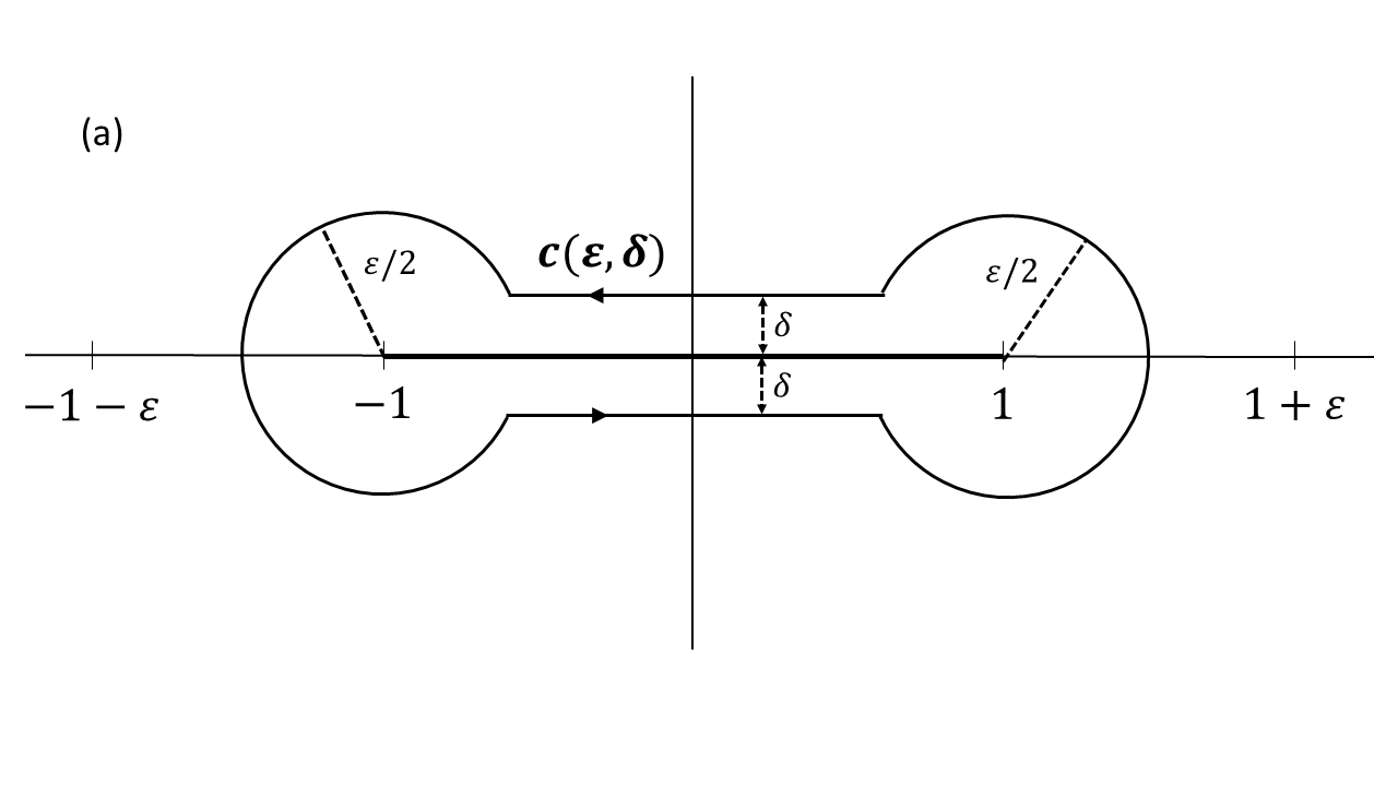
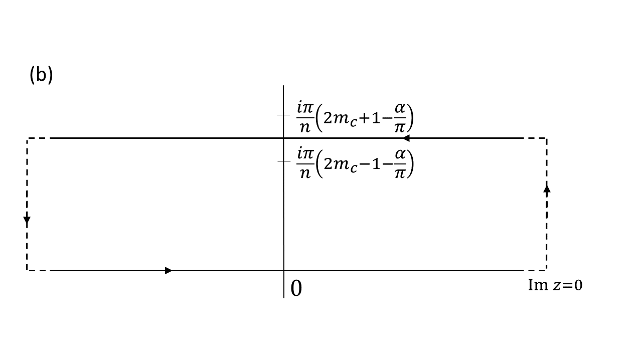
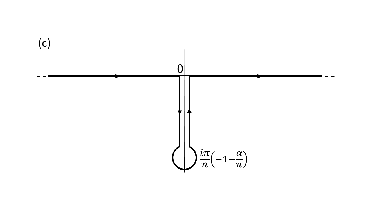
Figure 1: (a) The integration contour $c\left(\varepsilon,\delta\right)$ used in (48). (b) The integration contour for the calculation of $I_{k}^{+}$ in (64). The broken vertical lines represent segments which are infinitely far from the imaginary line. (c) The deformed integration contour used in the calculation of $\Upsilon_{0,a}\left(n,\alpha+2\pi\right)$ in (71).

We begin by omitting subleading contributions to the asymptotic expression for $D_{L}\left(\lambda\right)$, substituting for it the leading order approximation (38). We will accordingly obtain a leading order approximation for $\ln S_{n}\left(\alpha\right)$ at large $L$; this approximation will be denoted by $\ln S_{n}^{\left(0\right)}\left(\alpha\right)$. One can show that

$$\frac{d}{d\lambda}\ln D_{L}^{\left(0\right)}\left(\lambda\right)=\left(\frac{k_{F}/\pi}{\lambda-1}+\frac{1-k_{F}/\pi}{\lambda+1}\right)L-\frac{4i}{\pi}\cdot\frac{\beta\left(\lambda\right)}{\left(\lambda+1\right)\left(\lambda-1\right)}\left[\ln\mathcal{L}+\left(1+\gamma_{E}\right)+\Upsilon\left(\lambda\right)\right],$$ (50)

where

$$\Upsilon\left(\lambda\right)\equiv\underset{k=1}{\overset{\infty}{\sum}}\frac{k^{-1}\beta^{2}\left(\lambda\right)}{k^{2}-\beta^{2}\left(\lambda\right)}.$$ (51)

Substituting (50) into (48) we get

$$\ln S_{n}^{\left(0\right)}\left(\alpha\right) =i\frac{\alpha}{2}L+\underset{\varepsilon,\delta\rightarrow 0^{+}}{\lim}\frac{1}{2\pi i}\underset{c\left(\varepsilon,\delta\right)}{\int}e_{n}^{\left(\alpha\right)}\left(1+\varepsilon,\lambda\right)\left(\frac{k_{F}/\pi}{\lambda-1}+\frac{1-k_{F}/\pi}{\lambda+1}\right)Ld\lambda+$$

$$+\underset{\varepsilon,\delta\rightarrow 0^{+}}{\lim}\frac{1}{2\pi i}\underset{c\left(\varepsilon,\delta\right)}{\int}e_{n}^{\left(\alpha\right)}\left(1+\varepsilon,\lambda\right)\left(-\frac{4i}{\pi}\cdot\frac{\beta\left(\lambda\right)}{\left(\lambda+1\right)\left(\lambda-1\right)}\left[\ln\mathcal{L}+\left(1+\gamma_{E}\right)+\Upsilon\left(\lambda\right)\right]\right)d\lambda.$$ (52)

Calculating the integrals, we obtain

$$\ln S_{n}^{\left(0\right)}\left(\alpha\right)=i\frac{k_{F}}{\pi}\alpha L+\left[\frac{1}{6}\left(\frac{1}{n}-n\right)-\frac{\alpha^{2}}{2\pi^{2}n}\right]\ln\mathcal{L}+\Upsilon_{0}\left(n,\alpha\right)\,\,\,\left(-\pi<\alpha<\pi\right),$$ (53)

where we have defined

$$\Upsilon_{0}\left(n,\alpha\right)\equiv-\frac{1}{\pi^{2}}\underset{0}{\overset{\infty}{\int}}\ln\left[\frac{2\cos\alpha+2\cosh\left(nu\right)}{\left(2\cosh\left(\frac{u}{2}\right)\right)^{2n}}\right]du\underset{0}{\overset{\infty}{\int}}\left[\frac{e^{-t}}{t}-\frac{\cos\left(\frac{ut}{2\pi}\right)}{2\sinh\left(\frac{t}{2}\right)}\right]dt.$$ (54)

An equivalent expression for $\Upsilon_{0}\left(n,\alpha\right)$, which will be of use later on, is

$$\Upsilon_{0}\left(n,\alpha\right)=\frac{in}{2\pi}\underset{-\infty}{\overset{\infty}{\int}}\left[\tanh\left(\frac{nu}{2}+i\frac{\alpha}{2}\right)-\tanh\left(\frac{u}{2}\right)\right]\ln\frac{\Gamma\left(\frac{1}{2}+\frac{u}{2\pi i}\right)}{\Gamma\left(\frac{1}{2}-\frac{u}{2\pi i}\right)}du.$$ (55)

It is important to note that the $\alpha^{2}$ term in (53) arises from a Fourier series, $\alpha^{2}=\frac{\pi^{2}}{3}+4\underset{k=1}{\overset{\infty}{\sum}}\frac{\left(-1\right)^{k}}{k^{2}}\cos\left(k\alpha\right)$, and therefore it should actually be continued periodically outside the interval $\left[-\pi,\pi\right]$. The calculation of (53) is detailed in subsection A.2 of the appendix.

It is noteworthy that the term $\Upsilon_{0}\left(n,\alpha\right)$ is independent of $L$ and $k_{F}$, and that it is real and even with respect to $\alpha$. We can therefore write

$$\Upsilon_{0}\left(n,\alpha\right)=c_{0}\left(n\right)+c_{2}\left(n\right)\alpha^{2}+\mathcal{O}\left(\alpha^{4}\right).$$ (56)

Knowing the values $c_{0}\left(n\right)$ and $c_{2}\left(n\right)$ lets us write $\ln S_{n}^{\left(0\right)}\left(\alpha\right)$ as a quadratic polynomial in $\alpha$:

$$\ln S_{n}^{\left(0\right)}\left(\alpha\right)\approx c_{0}\left(n\right)+\frac{1}{6}\left(\frac{1}{n}-n\right)\ln\mathcal{L}+i\frac{k_{F}}{\pi}L\alpha-\frac{1}{2}\left(\frac{\ln\mathcal{L}}{\pi^{2}n}-2c_{2}\left(n\right)\right)\alpha^{2}\equiv\ln S_{n}^{\left(G\right)}\left(\alpha\right),$$ (57)

In such a way the flux-resolved REE is approximated (up to a phase and a normalization constant) as a density function of a Gaussian distribution $S_{n}^{\left(G\right)}\left(\alpha\right)$, which implies that under this approximation its Fourier transform — the charge-resolved REE — represents a Gaussian distribution as well:

$$S_{n}\left(Q_{A}\right)\approx e^{c_{0}\left(n\right)}{\cal L}^{\frac{1}{6}\left(\frac{1}{n}-n\right)}\sqrt{\frac{1}{\frac{2\ln\mathcal{L}}{\pi n}-4\pi c_{2}\left(n\right)}}\exp\left[-\frac{\pi\left(Q_{A}-\frac{k_{F}}{\pi}L\right)^{2}}{\frac{2\ln\mathcal{L}}{\pi n}-4\pi c_{2}\left(n\right)}\right].$$ (58)

The deviation of $S_{n}^{\left(G\right)}\left(\alpha\right)$ from $S_{n}^{\left(0\right)}\left(\alpha\right)$ is obviously small as long as $\left|\alpha\right|\ll\pi$. If we demand that $\ln\mathcal{L}/n\gg 1$, subleading corrections to $S_{n}^{\left(0\right)}\left(\alpha\right)$ do not spoil this (for $\left|\alpha\right|\ll\pi$ these subleading corrections, which we obtain below, vanish exponentially as $\ln\mathcal{L}/n\rightarrow\infty$), meaning that $S_{n}\left(\alpha\right)\approx S_{n}^{\left(G\right)}\left(\alpha\right)$ constitutes a decent approximation in the $\left|\alpha\right|\ll\pi$ regime. Furthermore, the condition $\ln\mathcal{L}/n\gg 1$ guarantees that the main contribution to the integral in (8) will come from the $\left|\alpha\right|\ll\pi$ regime, due to the fast decay of the $\exp\left[-\frac{1}{2}\left(\frac{\ln\mathcal{L}}{\pi^{2}n}-2c_{2}\left(n\right)\right)\alpha^{2}\right]$ term away from $\alpha=0$. We can therefore deduce that the Gaussian approximation (58) is valid as long as $\ln\mathcal{L}/n\gg 1$. We will test the quality of this approximation in the next subsection.

The value of $c_{2}\left(n\right)$ for the case $n=1$ is of special interest: since $S_{1}\left(Q_{A}\right)$ is the charge distribution in subsystem $A$, the expression $\left(\frac{\ln\mathcal{L}}{\pi^{2}}-2c_{2}\left(1\right)\right)$ corresponds to the charge variance. Substituting $n=1$, the value $c_{2}\left(1\right)=-\frac{1+\gamma_{E}}{2\pi^{2}}$ is obtained (a detailed proof is presented in subsection A.3 of the appendix). This agrees with [52], where it was proven that for a half-filled chain ($k_{F}=\frac{\pi}{2}$, and accordingly $\mathcal{L}=2L$) the charge variance is $\frac{\ln 2L+1+\gamma_{E}}{\pi^{2}}$.

4.2 Corrections up to the order of ${\cal O}\left(\mathcal{L}^{-1}\right)$

Corrections to the leading order approximation (53) can be calculated by taking into account subleading contributions that appear in (39). Following [46], we use the fact that $G\left(1+x\right)/G\left(x\right)=\Gamma\left(x\right)$ and, omitting terms which will contribute corrections of order $\mathcal{O}\left(\mathcal{L}^{-4}\right)$, we rewrite (39) as

$$D_{L}\left(\lambda\right) =D_{L}^{\left(0\right)}\left(\lambda\right)\left[1+e^{2ik_{F}L}\mathcal{L}^{-2+4\beta\left(\lambda\right)}\frac{\Gamma\left(1-\beta\left(\lambda\right)\right)^{2}}{\Gamma\left(\beta\left(\lambda\right)\right)^{2}}+e^{-2ik_{F}L}\mathcal{L}^{-2-4\beta\left(\lambda\right)}\frac{\Gamma\left(1+\beta\left(\lambda\right)\right)^{2}}{\Gamma\left(-\beta\left(\lambda\right)\right)^{2}}\right]\equiv$$

$$\equiv D_{L}^{\left(0\right)}\left(\lambda\right)\left[1+H\left(\lambda\right)\right].$$ (59)

Substituting this into the integral expression for $\ln S_{n}\left(\alpha\right)$ (48), we obtain

$$\ln S_{n}\left(\alpha\right) =\ln S_{n}^{\left(0\right)}\left(\alpha\right)+\underset{\varepsilon,\delta\rightarrow 0^{+}}{\lim}\frac{1}{2\pi i}\underset{c\left(\varepsilon,\delta\right)}{\int}e_{n}^{\left(\alpha\right)}\left(1+\varepsilon,\lambda\right)\frac{d}{d\lambda}\ln\left[1+H\left(\lambda\right)\right]d\lambda+\mathcal{O}\left(\mathcal{L}^{-4}\right)=$$

$$=\ln S_{n}^{\left(0\right)}\left(\alpha\right)-\underset{\varepsilon,\delta\rightarrow 0^{+}}{\lim}\frac{1}{2\pi i}\underset{c\left(\varepsilon,\delta\right)}{\int}\frac{de_{n}^{\left(\alpha\right)}\left(1+\varepsilon,\lambda\right)}{d\lambda}\ln\left[1+H\left(\lambda\right)\right]d\lambda+\mathcal{O}\left(\mathcal{L}^{-4}\right).$$ (60)

Using the fact that for every $-1<x<1$,

$$\beta\left(x+i0^{\pm}\right)=-iW\left(x\right)\mp\frac{1}{2},$$ (61)

where $W\left(x\right)\equiv\frac{1}{2\pi}\ln\frac{1+x}{1-x}$, we obtain that

$$H\left(x+i0^{\pm}\right)=e^{\pm 2i\left(2\ln\mathcal{L}W\left(x\right)-k_{F}L\right)}\frac{\Gamma\left(\frac{1}{2}\mp iW\left(x\right)\right)^{2}}{\Gamma\left(\frac{1}{2}\pm iW\left(x\right)\right)^{2}}+\mathcal{O}\left(\mathcal{L}^{-4}\right).$$ (62)

Now we write $\ln\left[1+H\left(\lambda\right)\right]=\underset{k=1}{\overset{\infty}{\sum}}\frac{\left(-1\right)^{k+1}}{k}H\left(\lambda\right)^{k}$ and take the limit $\varepsilon,\delta\rightarrow 0^{+}$, omitting terms of order $\mathcal{O}\left(\mathcal{L}^{-4}\right)$, so that we get

$$\ln S_{n}\left(\alpha\right)-\ln S_{n}^{\left(0\right)}\left(\alpha\right) =\frac{1}{2\pi i}\underset{-\infty}{\overset{\infty}{\int}}du\underset{k=1}{\overset{\infty}{\sum}}\frac{\left(-1\right)^{k+1}n}{2k}\left[\tanh\left(\frac{nu}{2}+i\frac{\alpha}{2}\right)-\tanh\left(\frac{u}{2}\right)\right]\times$$

$$\times\left\{e^{2ik\left(\frac{\ln\mathcal{L}}{\pi}u-k_{F}L\right)}\frac{\Gamma\left(\frac{1}{2}+\frac{u}{2\pi i}\right)^{2k}}{\Gamma\left(\frac{1}{2}-\frac{u}{2\pi i}\right)^{2k}}-e^{-2ik\left(\frac{\ln\mathcal{L}}{\pi}u-k_{F}L\right)}\frac{\Gamma\left(\frac{1}{2}-\frac{u}{2\pi i}\right)^{2k}}{\Gamma\left(\frac{1}{2}+\frac{u}{2\pi i}\right)^{2k}}\right\}.$$ (63)

Let us define a natural number $m_{c}=m_{c}\left(n\right)\equiv\lceil\frac{n}{4}\rceil+1$, so that $m_{c}\geq\frac{n}{4}+1$, and thus $\frac{2}{n}\left(2m_{c}-1\pm\frac{\alpha}{\pi}\right)\geq 1$ for every $-\pi<\alpha<\pi$. For each $k\geq 1$ and every $-\pi<\alpha<\pi$, we can estimate the integral

$$I_{k}^{+}\equiv\frac{1}{2\pi i}\underset{-\infty}{\overset{\infty}{\int}}du\frac{\left(-1\right)^{k+1}n}{2k}\left[\tanh\left(\frac{nu}{2}+i\frac{\alpha}{2}\right)-\tanh\left(\frac{u}{2}\right)\right]e^{2ik\left(\frac{\ln\mathcal{L}}{\pi}u-k_{F}L\right)}\frac{\Gamma\left(\frac{1}{2}+\frac{u}{2\pi i}\right)^{2k}}{\Gamma\left(\frac{1}{2}-\frac{u}{2\pi i}\right)^{2k}}$$ (64)

by enclosing the $m_{c}$ poles of $\tanh\left(\frac{nz}{2}+i\frac{\alpha}{2}\right)$ that are in the upper half-plane (at $z=\frac{i\pi}{n}\left(2m-1-\frac{\alpha}{\pi}\right)$ for $m\in\mathbb{N}$) and are closest to the real line using a rectangular contour, the vertical sides of which are infinitely far from the imaginary line, and whose upper horizontal side crosses the imaginary line through the segment between the $m_{c}$-th and the $\left(m_{c}+1\right)$-th pole of $\tanh\left(\frac{nz}{2}+i\frac{\alpha}{2}\right)$ (see Fig. 1(b)). Thus we make sure that the integral over the upper horizontal side of the contour is of order $\mathcal{O}\left(\mathcal{L}^{-1-\frac{4}{n}}\right)$ at most. Ignoring the poles of $\tanh\left(\frac{z}{2}\right)$, considering that the contribution of their residues is only of order $\mathcal{O}\left(\mathcal{L}^{-2}\right)$, we can write

$$I_{k}^{+}=\underset{m=1}{\overset{m_{c}}{\sum}}\frac{\left(-1\right)^{k+1}}{k}\mathcal{L}^{-\frac{2k}{n}\left(2m-1-\frac{\alpha}{\pi}\right)}e^{-2ik_{F}Lk}\frac{\Gamma\left(\frac{1}{2}+\frac{1}{2n}\left(2m-1-\frac{\alpha}{\pi}\right)\right)^{2k}}{\Gamma\left(\frac{1}{2}-\frac{1}{2n}\left(2m-1-\frac{\alpha}{\pi}\right)\right)^{2k}}+\mathcal{O}\left(\mathcal{L}^{-1-\frac{4}{n}}+\mathcal{L}^{-2}\right).$$ (65)

In a similar way, we define

$$I_{k}^{-}\equiv-\frac{1}{2\pi i}\underset{-\infty}{\overset{\infty}{\int}}du\frac{\left(-1\right)^{k+1}n}{2k}\left[\tanh\left(\frac{nu}{2}+i\frac{\alpha}{2}\right)-\tanh\left(\frac{u}{2}\right)\right]e^{-2ik\left(\frac{\ln\mathcal{L}}{\pi}u-k_{F}L\right)}\frac{\Gamma\left(\frac{1}{2}-\frac{u}{2\pi i}\right)^{2k}}{\Gamma\left(\frac{1}{2}+\frac{u}{2\pi i}\right)^{2k}},$$ (66)

and sum over the residues of $\tanh\left(\frac{nz}{2}+i\frac{\alpha}{2}\right)$ at its poles in the lower half-plane up to $m=m_{c}$, so that we get

$$I_{k}^{-}=\underset{m=1}{\overset{m_{c}}{\sum}}\frac{\left(-1\right)^{k+1}}{k}\mathcal{L}^{-\frac{2k}{n}\left(2m-1+\frac{\alpha}{\pi}\right)}e^{2ik_{F}Lk}\frac{\Gamma\left(\frac{1}{2}+\frac{1}{2n}\left(2m-1+\frac{\alpha}{\pi}\right)\right)^{2k}}{\Gamma\left(\frac{1}{2}-\frac{1}{2n}\left(2m-1+\frac{\alpha}{\pi}\right)\right)^{2k}}+\mathcal{O}\left(\mathcal{L}^{-1-\frac{4}{n}}+\mathcal{L}^{-2}\right).$$ (67)

The summation over $m$ is truncated due the fact that infinite summation will not converge. Further corrections of order $o\left(\mathcal{L}^{-1}\right)$ that are not captured by the generalized Fisher-Hartwig conjecture, and stem from a calculation related to random matrix theory, were found in the calculation of the total REE in [46].

Summing over $k$, we finally get

$$\ln S_{n}\left(\alpha\right)=\ln S_{n}^{\left(0\right)}\left(\alpha\right)+\Upsilon_{1}\left(n,\alpha,L,k_{F}\right)+o\left(\mathcal{L}^{-1}\right)\,\,\,\left(-\pi<\alpha<\pi\right),$$ (68)

where

$$\Upsilon_{1}\left(n,\alpha,L,k_{F}\right) \equiv\underset{m=1}{\overset{m_{c}}{\sum}}\ln\left[1+\mathcal{L}^{-\frac{2}{n}\left(2m-1-\frac{\alpha}{\pi}\right)}e^{-2ik_{F}L}\frac{\Gamma\left(\frac{1}{2}+\frac{1}{2n}\left(2m-1-\frac{\alpha}{\pi}\right)\right)^{2}}{\Gamma\left(\frac{1}{2}-\frac{1}{2n}\left(2m-1-\frac{\alpha}{\pi}\right)\right)^{2}}\right]+$$

$$+\underset{m=1}{\overset{m_{c}}{\sum}}\ln\left[1+\mathcal{L}^{-\frac{2}{n}\left(2m-1+\frac{\alpha}{\pi}\right)}e^{2ik_{F}L}\frac{\Gamma\left(\frac{1}{2}+\frac{1}{2n}\left(2m-1+\frac{\alpha}{\pi}\right)\right)^{2}}{\Gamma\left(\frac{1}{2}-\frac{1}{2n}\left(2m-1+\frac{\alpha}{\pi}\right)\right)^{2}}\right].$$ (69)

Fig. 2(a) shows the dependence of the flux-resolved REE on $\alpha$ in a half-filled system ($k_{F}=\frac{\pi}{2}$), for different values of $n$. The numerical evaluation of (47) is compared to the analytical results, and it can be seen that while the leading order approximation $S_{n}^{\left(0\right)}\left(\alpha\right)$ exhibits an $\mathcal{O}\left(1\right)$ deviation from the numerical values as $\alpha\rightarrow\pm\pi$, this deviation practically vanishes after we include corrections up to order ${\cal O}\left({\cal L}^{-1}\right)$. Fig. 2(b) shows a more detailed comparison between the analytical result up to order $\mathcal{O}\left(\mathcal{L}^{-1}\right)$ and the numerical result, for the case of half-filling. In this figure we denote the analytical result by $\ln S_{n}^{\left(1\right)}\left(\alpha\right)\equiv\ln S_{n}^{\left(0\right)}\left(\alpha\right)+\Upsilon_{1}\left(n,\alpha,L,k_{F}\right)$, while the numerical result is denoted by $\ln S_{n}\left(\alpha\right)$. The negligible difference between the two calculations indicates that $\ln S_{n}^{\left(1\right)}\left(\alpha\right)$ provides a very good approximation even for a subsystem of relatively moderate length.

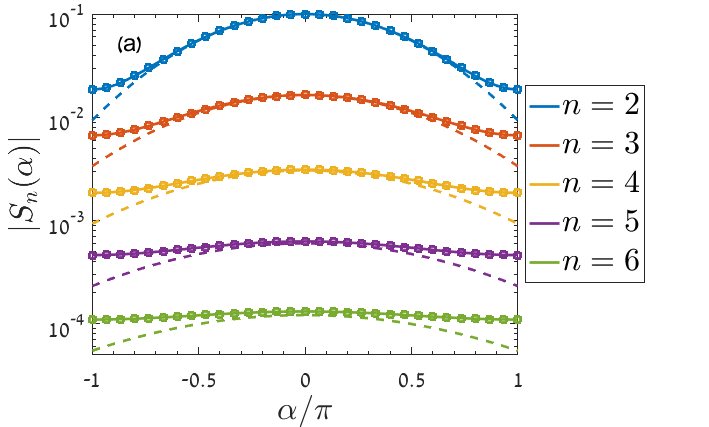
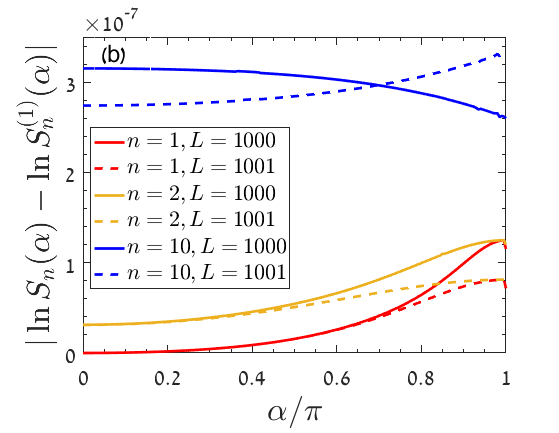
Figure 2: (a) Flux-resolved REE in a subsystem of length $L=1000$ of a half-filled gapless XX chain, computed numerically according to (47) (dots), using the analytical leading order approximation (53) (broken lines), and using the analytical approximation up to ${\cal O}\left({\cal L}^{-1}\right)$ (68) (continuous lines). (b) The absolute deviation of the analytical result up to order $\mathcal{O}\left(\mathcal{L}^{-1}\right)$ from the numerical result for the flux-resolved REE, for a half-filled gapless XX chain.

We can now use the analytical results for $S_{n}\left(\alpha\right)$ in order to calculate the charge-resolved REE through (8), and then the charge-resolved vNEE. Fig. 3 shows that when we use the analytical approximation $S_{n}^{\left(1\right)}\left(\alpha\right)$, these calculations are in good agreement with numerical results. On the other hand, the Gaussian approximation derived from (58) exhibits a discernible deviation from numerical results for both $S_{1}\left(Q_{A}\right)$ and ${\cal S}\left(Q_{A}\right)$, since $\ln\mathcal{L}$ is not large enough.

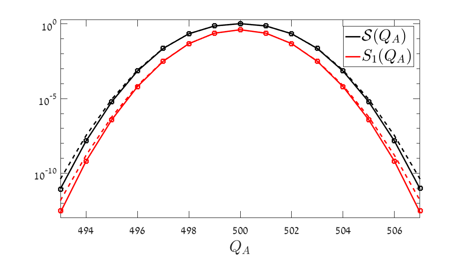
Figure 3: Charge-resolved REE and vNEE in a subsystem of length $L=1000$ of a half-filled gapless XX chain, computed numerically according to (47) and (8) (dots), using the analytical Gaussian approximation (58) (broken lines), and using the analytical approximation up to ${\cal O}\left({\cal L}^{-1}\right)$ according to (68) and (8) (continuous lines).

4.3 Periodic structure up to the order of ${\cal O}\left(\mathcal{L}^{-1}\right)$

$\ln S_{n}^{\left(0\right)}\left(\alpha\right)$ in (53) was defined for $-\pi<\alpha<\pi$, and its real part is $2\pi$-periodic in $\alpha$ (remember that the $\alpha^{2}$ term originated from a Fourier series). Nevertheless, its periodic continuation is not analytic (nor is it even differentiable), so we would like to define the analytic continuation of $S_{n}^{\left(0\right)}\left(\alpha\right)$ for $\alpha\in\mathbb{R}$. For this purpose, we will construct a natural continuation of $\ln S_{n}^{\left(0\right)}\left(\alpha\right)$ so that the corresponding continuation of $S_{n}^{\left(0\right)}\left(\alpha\right)$, which will be denoted by $S_{a,n}^{\left(0\right)}\left(\alpha\right)$, would turn out analytic. The linear and quadratic terms in (53) naturally remain as before, so we need only to construct an appropriate continuation $\Upsilon_{0,a}\left(n,\alpha\right)$ of the term $\Upsilon_{0}\left(n,\alpha\right)$, and then obtain for $\alpha\in\mathbb{R}$

$$S_{a,n}^{\left(0\right)}\left(\alpha\right)=\exp\left\{i\frac{k_{F}}{\pi}\alpha L+\left[\frac{1}{6}\left(\frac{1}{n}-n\right)-\frac{\alpha^{2}}{2\pi^{2}n}\right]\ln\mathcal{L}+\Upsilon_{0,a}\left(n,\alpha\right)\right\}.$$ (70)

Regarding the term $\Upsilon_{0}\left(n,\alpha\right)$ as it is written in (55), note that as $\alpha$ approaches $\pi^{-}$ or $-\pi^{+}$, a pole of the function $\tanh\left(\frac{nz}{2}+i\frac{\alpha}{2}\right)$ approaches the real line. A shift of $\alpha\rightarrow\alpha+2\pi$ maintains the positions of all poles of $\tanh\left(\frac{nz}{2}+i\frac{\alpha}{2}\right)$ in the upper half-plane (at $z=\frac{i\pi}{n}\left(2m-1-\frac{\alpha}{\pi}\right),\,m\in\mathbb{N}$), but during a continuous shift of such kind the pole that was originally at $z=\frac{i\pi}{n}\left(1-\frac{\alpha}{\pi}\right)$ crosses the real line, and ends up at $z=\frac{i\pi}{n}\left(-1-\frac{\alpha}{\pi}\right)$. We can now think of $\Upsilon_{0,a}\left(n,\alpha+2\pi\right)$ as the value obtained by calculating the integral in (55) while deforming the contour of integration (originally just the real line) so that it also encircles the pole that crossed the real line, thus counting the residue of the integrand at $z=\frac{i\pi}{n}\left(-1-\frac{\alpha}{\pi}\right)$ (see Fig. 1(c)). In such a way we get for every $-\pi<\alpha<\pi$,

$$\Upsilon_{0,a}\left(n,\alpha+2\pi\right)-\Upsilon_{0}\left(n,\alpha\right) =\text{Res}\left\{-n\left[\tanh\left(\frac{nz}{2}+i\frac{\alpha}{2}\right)-\tanh\left(\frac{z}{2}\right)\right]\ln\frac{\Gamma\left(\frac{1}{2}+\frac{z}{2\pi i}\right)}{\Gamma\left(\frac{1}{2}-\frac{z}{2\pi i}\right)},z=\frac{i\pi}{n}\left(-1-\frac{\alpha}{\pi}\right)\right\}=$$

$$=2\ln\frac{\Gamma\left(\frac{1}{2}+\frac{1}{2n}\left(1+\frac{\alpha}{\pi}\right)\right)}{\Gamma\left(\frac{1}{2}-\frac{1}{2n}\left(1+\frac{\alpha}{\pi}\right)\right)}.$$ (71)

By the same logic, for every natural number $m\geq 1$ we can deform the integration contour so that it encircles the $m$ poles which cross the real line from the upper half-plane to the lower half-plane during the shift $\alpha\rightarrow\alpha+2\pi m$, so that for every $-\pi<\alpha<\pi$,

$$\Upsilon_{0,a}\left(n,\alpha+2\pi m\right)-\Upsilon_{0}\left(n,\alpha\right) =\underset{j=1}{\overset{m}{\sum}}\text{Res}\left\{-n\left[\tanh\left(\frac{nz}{2}+i\frac{\alpha}{2}\right)-\tanh\left(\frac{z}{2}\right)\right]\ln\frac{\Gamma\left(\frac{1}{2}+\frac{z}{2\pi i}\right)}{\Gamma\left(\frac{1}{2}-\frac{z}{2\pi i}\right)},z=\frac{i\pi}{n}\left(-2j+1-\frac{\alpha}{\pi}\right)\right\}=$$

$$=\underset{j=1}{\overset{m}{\sum}}2\ln\frac{\Gamma\left(\frac{1}{2}+\frac{1}{2n}\left(2j-1+\frac{\alpha}{\pi}\right)\right)}{\Gamma\left(\frac{1}{2}-\frac{1}{2n}\left(2j-1+\frac{\alpha}{\pi}\right)\right)}.$$ (72)

For a shift of $\alpha\rightarrow\alpha-2\pi m$ (this time encircling poles that cross the real line from the lower half-plane to the upper half-plane), we get for every $-\pi<\alpha<\pi$,

$$\Upsilon_{0,a}\left(n,\alpha-2\pi m\right)-\Upsilon_{0}\left(n,\alpha\right)=\underset{j=1}{\overset{m}{\sum}}2\ln\frac{\Gamma\left(\frac{1}{2}+\frac{1}{2n}\left(2j-1-\frac{\alpha}{\pi}\right)\right)}{\Gamma\left(\frac{1}{2}-\frac{1}{2n}\left(2j-1-\frac{\alpha}{\pi}\right)\right)}.$$ (73)

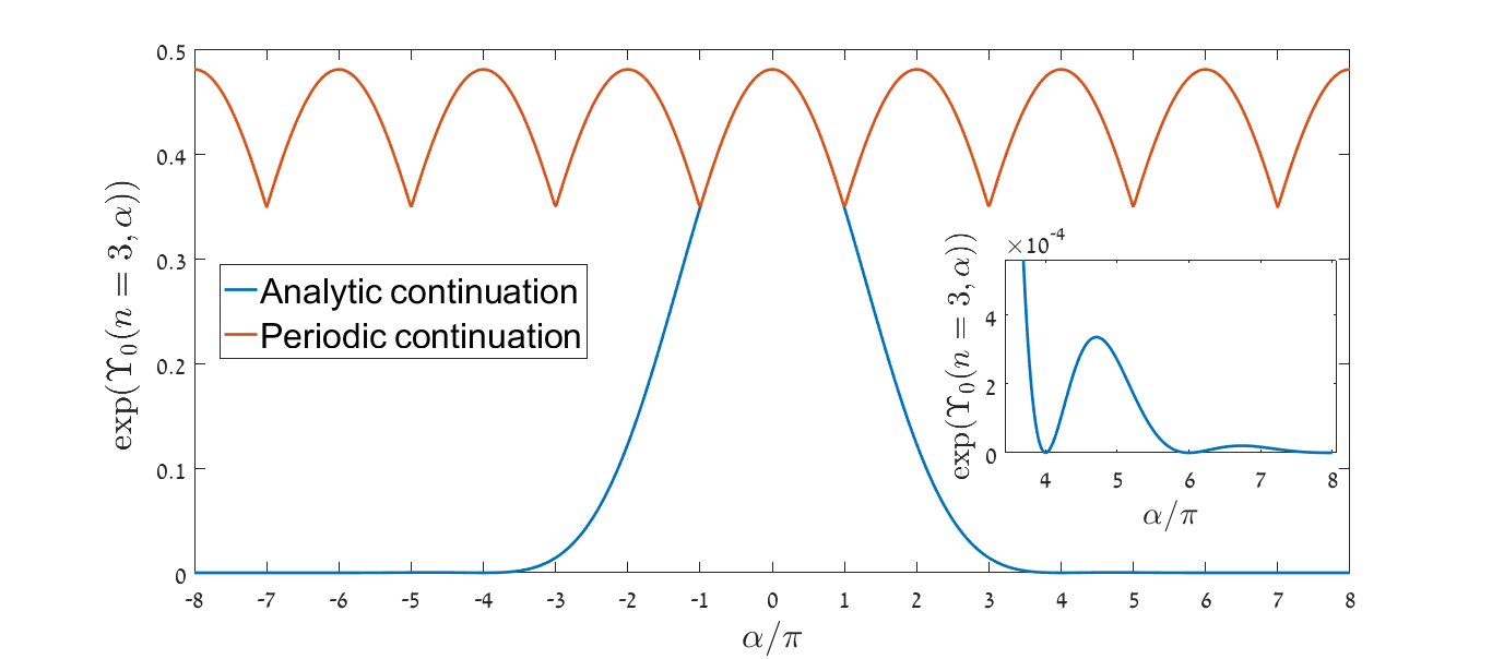
Figure 4: Continuation of $\exp\left(\Upsilon_{0}\left(n,\alpha\right)\right)$ for $n=3$. Inset shows a zoomed-in view of the tail of the analytic continuation $\exp\left(\Upsilon_{0,a}\left(n=3,\alpha\right)\right)$.

For fixed $n$, the terms $\Gamma\left(\frac{1}{2}-\frac{1}{2n}\left(2j-1\pm\frac{\alpha}{\pi}\right)\right)$ might diverge for certain values of $j$ and $\alpha$, in which case (72) or (73) diverge, respectively. This however does not pose a problem, since we are eventually interested in the exponents of (72) and (73), and when $\Gamma\left(\frac{1}{2}-\frac{1}{2n}\left(2j-1\pm\frac{\alpha}{\pi}\right)\right)$ diverge for some $1\leq j\leq m$ it just means that $\exp\left(\Upsilon_{0,a}\left(n,\alpha\pm 2\pi m\right)\right)=0$, respectively. Both the periodic and the analytic contintuations of $\exp\Upsilon_{0}$ are presented in Fig. 4.

Defining $\Upsilon_{0,a}\left(n,\alpha\right)$ this way and substituting it into the analytic continuation of $S_{n}^{\left(0\right)}\left(\alpha\right)$ in (70), we obtain for each $m\in\mathbb{N}$ and every $-\pi<\alpha<\pi$,

$$\frac{S_{a,n}^{\left(0\right)}\left(\alpha\pm 2\pi m\right)}{S_{n}^{\left(0\right)}\left(\alpha\right)}=\mathcal{L}^{-\frac{2}{n}\left(m^{2}\pm\frac{\alpha}{\pi}m\right)}e^{\pm 2imk_{F}L}\underset{j=1}{\overset{m}{\Pi}}\frac{\Gamma\left(\frac{1}{2}+\frac{1}{2n}\left(2j-1\pm\frac{\alpha}{\pi}\right)\right)^{2}}{\Gamma\left(\frac{1}{2}-\frac{1}{2n}\left(2j-1\pm\alpha\right)\right)^{2}},$$ (74)

and in particular

$$\frac{S_{a,n}^{\left(0\right)}\left(\alpha+2\pi m\right)}{S_{a,n}^{\left(0\right)}\left(\alpha+2\pi\left(m-1\right)\right)} =\mathcal{L}^{-\frac{2}{n}\left(2m-1+\frac{\alpha}{\pi}\right)}e^{2ik_{F}L}\frac{\Gamma\left(\frac{1}{2}+\frac{1}{2n}\left(2m-1+\frac{\alpha}{\pi}\right)\right)^{2}}{\Gamma\left(\frac{1}{2}-\frac{1}{2n}\left(2m-1+\frac{\alpha}{\pi}\right)\right)^{2}},$$

$$\frac{S_{a,n}^{\left(0\right)}\left(\alpha-2\pi m\right)}{S_{a,n}^{\left(0\right)}\left(\alpha-2\pi\left(m-1\right)\right)} =\mathcal{L}^{-\frac{2}{n}\left(2m-1-\frac{\alpha}{\pi}\right)}e^{-2ik_{F}L}\frac{\Gamma\left(\frac{1}{2}+\frac{1}{2n}\left(2m-1-\frac{\alpha}{\pi}\right)\right)^{2}}{\Gamma\left(\frac{1}{2}-\frac{1}{2n}\left(2m-1-\frac{\alpha}{\pi}\right)\right)^{2}}.$$ (75)

Let us now define $\sigma_{m}\left(\alpha\right)\equiv S_{a,n}^{\left(0\right)}\left(\alpha+2\pi m\right)$ for every $m\in\mathbb{Z}$ and $-\pi<\alpha<\pi$. We can rewrite (68) as

$$\ln S_{n}\left(\alpha\right)=\ln\sigma_{0}\left(\alpha\right)+\underset{m=1}{\overset{m_{c}}{\sum}}\left\{\ln\left[1+\frac{\sigma_{m}\left(\alpha\right)}{\sigma_{m-1}\left(\alpha\right)}\right]+\ln\left[1+\frac{\sigma_{-m}\left(\alpha\right)}{\sigma_{-m+1}\left(\alpha\right)}\right]\right\}+o\left(\mathcal{L}^{-1}\right),$$ (76)

and therefore, up to $o\left(\mathcal{L}^{-1}\right)$ corrections,

$$S_{n}\left(\alpha\right)=\left[\underset{m=1}{\overset{m_{c}}{\Pi}}\left(\frac{\sigma_{-m}\left(\alpha\right)}{\sigma_{-m+1}\left(\alpha\right)}+1\right)\right]\sigma_{0}\left(\alpha\right)\left[\underset{m=1}{\overset{m_{c}}{\Pi}}\left(1+\frac{\sigma_{m}\left(\alpha\right)}{\sigma_{m-1}\left(\alpha\right)}\right)\right].$$ (77)

We could have formally represented the result in (68) as an asymptotic (divergent) series had we not defined the cutoff index $m_{c}$. Such a representation would have brought us to the asymptotic (divergent) product

$$S_{n}\left(\alpha\right)=\left[\underset{m=1}{\overset{\infty}{\Pi}}\left(\frac{\sigma_{-m}\left(\alpha\right)}{\sigma_{-m+1}\left(\alpha\right)}+1\right)\right]\sigma_{0}\left(\alpha\right)\left[\underset{m=1}{\overset{\infty}{\Pi}}\left(1+\frac{\sigma_{m}\left(\alpha\right)}{\sigma_{m-1}\left(\alpha\right)}\right)\right],$$ (78)

which for any arbitrary $j\in\mathbb{Z}$ can be written as

$$S_{n}\left(\alpha\right)=\left[\underset{m=1}{\overset{\infty}{\Pi}}\left(\frac{\sigma_{j-m}\left(\alpha\right)}{\sigma_{j-m+1}\left(\alpha\right)}+1\right)\right]\sigma_{j}\left(\alpha\right)\left[\underset{m=1}{\overset{\infty}{\Pi}}\left(1+\frac{\sigma_{j+m}\left(\alpha\right)}{\sigma_{j+m-1}\left(\alpha\right)}\right)\right].$$ (79)

This result is just $S_{n}\left(\alpha+2\pi j\right)=S_{n}\left(\alpha\right)$, as long as we ignore $o\left(\mathcal{L}^{-1}\right)$ corrections and treat it as an asymptotic product.

Note that the result in (77) can also be written as

$$S_{n}\left(\alpha\right)=\underset{j=-m_{c}}{\overset{m_{c}}{\sum}}S_{a,n}^{\left(0\right)}\left(\alpha+2\pi j\right)+o\left(1\right),$$ (80)

a structure which is natural from the CFT perspective. Indeed, there one writes the flux-resolved entropy $S_{n}\left(\alpha\right)$ as a correlation function over $n$ copies of space-time of $\mathcal{T}_{\mathcal{V}}=\mathcal{T}\times\mathcal{V}$, twist fields (appearing in the calculation of the total entropies) $\mathcal{T}$ modified by fusion of vertex operators $\mathcal{V}$, which assign a phase $\alpha$ to every particle encircling them [20]. In a bosonized language it can be written in terms of the appropriate boson field $\phi$ as $\mathcal{V}_{0}\left(\alpha\right)=e^{i\frac{\alpha}{2\pi}\phi}$. However, the periodicity in $\alpha$ implies that $\mathcal{V}$ could actually be taken as a sum over all possible shifts of $\alpha$ by integer multiples of $2\pi$, that is

$$\mathcal{T}_{\mathcal{V}}=\sum_{j}a_{j}(n,\alpha)\mathcal{T}\times\mathcal{V}_{0}(\alpha+2\pi j),$$ (81)

with some coefficients $a_{j}(n,\alpha)$. Computing the entropies as in [20] would then lead to the form of (80). Our exact results allow one to go beyond CFT and find the coefficients for the XX system, which take the values $a_{j}\left(n,\alpha\right)=\exp\Upsilon_{0,a}\left(n,\alpha+2\pi j\right)$.

Interestingly, this structure is maintained even when we include all terms up to an order of $\mathcal{O}\left(\mathcal{L}^{-1}\right)$. Let us define for every $-\pi<\alpha<\pi$

$$\sigma_{\mathrm{right}}\left(\alpha\right)\equiv\sigma_{0}\left(\alpha\right)\left[\underset{m=2}{\overset{m_{c}}{\Pi}}\left(1+\frac{\sigma_{m}\left(\alpha\right)}{\sigma_{m-1}\left(\alpha\right)}\right)\right].$$ (82)

First, note that (77) can be also written as

$$S_{n}\left(\alpha\right)=\sigma_{-m_{c}}\left(\alpha\right)\left[\underset{m=-m_{c}+1}{\overset{m_{c}}{\Pi}}\left(1+\frac{\sigma_{m}\left(\alpha\right)}{\sigma_{m-1}\left(\alpha\right)}\right)\right]=\underset{j=-m_{c}}{\overset{m_{c}}{\sum}}\sigma_{j}\left(\alpha\right)\underset{m=j+2}{\overset{m_{c}}{\Pi}}\left(1+\frac{\sigma_{m}\left(\alpha\right)}{\sigma_{m-1}\left(\alpha\right)}\right).$$ (83)

By definition of $m_{c}$, for any $m>m_{c}$ and every $-\pi<\alpha<\pi$ it is true that $\frac{\sigma_{m}\left(\alpha\right)}{\sigma_{m-1}\left(\alpha\right)}=o\left(\mathcal{L}^{-1}\right)$, and therefore for every $0\leq j\leq m_{c}$,

$$\sigma_{j}\left(\alpha\right)\underset{m=j+2}{\overset{m_{c}}{\Pi}}\left(1+\frac{\sigma_{m}\left(\alpha\right)}{\sigma_{m-1}\left(\alpha\right)}\right) =\sigma_{j}\left(\alpha\right)\underset{m=2}{\overset{m_{c}-j}{\Pi}}\left(1+\frac{\sigma_{j+m}\left(\alpha\right)}{\sigma_{j+m-1}\left(\alpha\right)}\right)=$$

$$=\sigma_{j}\left(\alpha\right)\underset{m=2}{\overset{m_{c}}{\Pi}}\left(1+\frac{\sigma_{j+m}\left(\alpha\right)}{\sigma_{j+m-1}\left(\alpha\right)}\right)+o\left(\mathcal{L}^{-1}\right)=$$

$$=\sigma_{\mathrm{right}}\left(\alpha+2\pi j\right)+o\left(\mathcal{L}^{-1}\right).$$ (84)

It is also evident from the relations in (75) that for $m_{1},m_{2}\geq 1$ such that $m_{1}+m_{2}>m_{c}$,

$$\frac{\sigma_{-m_{1}}\left(\alpha\right)}{\sigma_{-m_{1}-1}\left(\alpha\right)}\cdot\frac{\sigma_{m_{2}}\left(\alpha\right)}{\sigma_{m_{2}-1}\left(\alpha\right)}=o\left(\mathcal{L}^{-1}\right).$$ (85)

We can thus conclude that for every $-m_{c}\leq j<0$,

$$\sigma_{j}\left(\alpha\right)\underset{m=j+2}{\overset{m_{c}}{\Pi}}\left(1+\frac{\sigma_{m}\left(\alpha\right)}{\sigma_{m-1}\left(\alpha\right)}\right) =\sigma_{j}\left(\alpha\right)\underset{m=j+2}{\overset{m_{c}+j}{\Pi}}\left(1+\frac{\sigma_{m}\left(\alpha\right)}{\sigma_{m-1}\left(\alpha\right)}\right)+o\left(\mathcal{L}^{-1}\right)=$$

$$=\sigma_{\mathrm{right}}\left(\alpha+2\pi j\right)+o\left(\mathcal{L}^{-1}\right).$$ (86)

From (83), (84) and (86) we can now derive that

$$S_{n}\left(\alpha\right)=\underset{j=-m_{c}}{\overset{m_{c}}{\sum}}\sigma_{\mathrm{right}}\left(\alpha+2\pi j\right)+o\left(\mathcal{L}^{-1}\right).$$ (87)

The symmetry of the expression for $S_{n}\left(\alpha\right)$ in (77) obviously enables us to equivalently write

$$S_{n}\left(\alpha\right)=\underset{j=-m_{c}}{\overset{m_{c}}{\sum}}\sigma_{\mathrm{left}}\left(\alpha+2\pi j\right)+o\left(\mathcal{L}^{-1}\right),$$ (88)

where we have defined

$$\sigma_{\mathrm{left}}\left(\alpha\right)\equiv\sigma_{0}\left(\alpha\right)\left[\underset{m=2}{\overset{m_{c}}{\Pi}}\left(1+\frac{\sigma_{-m}\left(\alpha\right)}{\sigma_{-m+1}\left(\alpha\right)}\right)\right].$$ (89)

This means that we can define

$$\tilde{S}_{n}\left(\alpha\right)\equiv\frac{\sigma_{\mathrm{left}}\left(\alpha\right)+\sigma_{\mathrm{right}}\left(\alpha\right)}{2}=\frac{\sigma_{0}\left(\alpha\right)}{2}\left[\underset{m=2}{\overset{m_{c}}{\Pi}}\left(1+\frac{\sigma_{-m}\left(\alpha\right)}{\sigma_{-m+1}\left(\alpha\right)}\right)+\underset{m=2}{\overset{m_{c}}{\Pi}}\left(1+\frac{\sigma_{m}\left(\alpha\right)}{\sigma_{m-1}\left(\alpha\right)}\right)\right],$$ (90)

and obtain the desired structure, namely

$$S_{n}\left(\alpha\right)=\underset{j=-m_{c}}{\overset{m_{c}}{\sum}}\tilde{S}_{n}\left(\alpha+2\pi j\right)+o\left(\mathcal{L}^{-1}\right).$$ (91)

5 Symmetry-resolved EE for the XY model

We now derive the asymptotic behavior of the analog of the flux-resolved REE for the ground state of the XY model, namely the parity-resolved $S_{n}^{\left(-\right)}\equiv\text{Tr}\left(\rho_{A}^{n}\left(-1\right)^{\hat{Q}_{A}}\right)$. We assume for simplicity that $h\geq 0$. Using (34), we can write

$$S_{n}^{\left(\pm\right)}=\underset{m=1}{\overset{L}{\Pi}}\left[\left(\frac{1-\nu_{m}}{2}\right)^{n}\pm\left(\frac{1+\nu_{m}}{2}\right)^{n}\right],$$ (92)

where we also denoted $S_{n}^{\left(+\right)}\equiv S_{n}$. Note that in particular we can immediately deduce that $S_{1}^{\left(-\right)}=S_{2}^{\left(-\right)}$.

5.1 Gapped XY model

We first estimate $S_{n}^{\left(-\right)}$ at the limit $L\rightarrow\infty$ assuming that the system is gapped, i.e., $h\neq 2$. As was explained in 3.2.2, as $L\rightarrow\infty$ the values $\pm\nu_{m}$ converge in pairs to the values $\lambda_{l}$ defined in (45), which in turn depend on $h$.

The case $h<2$ is simple: since $\lambda_{0}=0$, we obtain $S_{n}^{\left(-\right)}\rightarrow 0$. For $h>2$, on the other hand, the asymptotic expression for $S_{n}^{\left(-\right)}$ does not vanish. Indeed, we can write

$$\underset{L\rightarrow\infty}{\lim}\underset{m=1}{\overset{L}{\Pi}}\left|\left(\frac{1-\nu_{m}}{2}\right)^{n}-\left(\frac{1+\nu_{m}}{2}\right)^{n}\right|= \underset{m=-\infty}{\overset{\infty}{\Pi}}\left|\left(\frac{1-\lambda_{m}}{2}\right)^{n}-\left(\frac{1+\lambda_{m}}{2}\right)^{n}\right|,$$ (93)

and writing $q\equiv e^{-\pi\tau_{0}}$ ($\tau_{0}$ was defined in (41)) we get

$$\underset{m=-\infty}{\overset{\infty}{\Pi}}\left|\left(\frac{1-\lambda_{m}}{2}\right)^{n}-\left(\frac{1+\lambda_{m}}{2}\right)^{n}\right|=\underset{m=0}{\overset{\infty}{\Pi}}\left[\left(\frac{1}{1+q^{2m+1}}\right)^{n}-\left(\frac{q^{2m+1}}{1+q^{2m+1}}\right)^{n}\right]^{2},$$ (94)

so that eventually we obtain

$$\underset{L\rightarrow\infty}{\lim}\left|S_{n}^{\left(-\right)}\right|=\underset{m=0}{\overset{\infty}{\Pi}}\left[\left(\frac{1}{1+q^{2m+1}}\right)^{n}-\left(\frac{q^{2m+1}}{1+q^{2m+1}}\right)^{n}\right]^{2}=\left(\frac{\underset{m=0}{\overset{\infty}{\Pi}}\left[1-q^{n\left(2m+1\right)}\right]}{\underset{m=0}{\overset{\infty}{\Pi}}\left[1+q^{\left(2m+1\right)}\right]^{n}}\right)^{2}.$$ (95)

In order to further simplify this result for $\underset{L\rightarrow\infty}{\lim}\left|S_{n}^{\left(-\right)}\right|$, we remind the reader of the definition of the Jacobi theta functions [49]:

$$\vartheta_{2}\left(z,q\right) =\underset{m=-\infty}{\overset{\infty}{\sum}}q^{\left(m+\frac{1}{2}\right)^{2}}e^{2iz\left(m+\frac{1}{2}\right)},$$

$$\vartheta_{3}\left(z,q\right) =\underset{m=-\infty}{\overset{\infty}{\sum}}q^{m^{2}}e^{2izm},$$

$$\vartheta_{4}\left(z,q\right) =\underset{m=-\infty}{\overset{\infty}{\sum}}\left(-1\right)^{m}q^{m^{2}}e^{2izm}.$$ (96)

We write $\theta_{j}\left(q\right)\equiv\vartheta_{j}\left(0,q\right)$ and

$$k\left(q\right)\equiv\frac{\theta_{2}^{2}\left(q\right)}{\theta_{3}^{2}\left(q\right)},\,\,\,k^{\prime}\left(q\right)\equiv\sqrt{1-k^{2}\left(q\right)}=\frac{\theta_{4}^{2}\left(q\right)}{\theta_{3}^{2}\left(q\right)}.$$ (97)

This definition of $k$ implies that $q=\exp\left[-\pi\frac{I\left(k^{\prime}\right)}{I\left(k\right)}\right]$ ($I$ was defined in (42)) [49], and thus it agrees with the definition of $k$ previously presented in (40). We also write $k_{n}\left(q\right)\equiv k\left(q^{n}\right)$ and $k_{n}^{\prime}\left(q\right)\equiv k^{\prime}\left(q^{n}\right)$, and rely on the following identities from [49] that hold for every $0<q<1$:

$$\underset{m=0}{\overset{\infty}{\Pi}}\left[1+q^{\left(2m+1\right)}\right] =\left(\frac{16q}{k^{2}k^{\prime 2}}\right)^{\frac{1}{24}},$$

$$\underset{m=0}{\overset{\infty}{\Pi}}\left[1-q^{\left(2m+1\right)}\right] =k^{\prime\frac{1}{4}}\underset{m=0}{\overset{\infty}{\Pi}}\left[1+q^{\left(2m+1\right)}\right]=\left(\frac{16qk^{\prime 4}}{k^{2}}\right)^{\frac{1}{24}}.$$ (98)

We then obtain that for $h>2$,

$$\underset{L\rightarrow\infty}{\lim}\left|S_{n}^{\left(-\right)}\right|=\left[\frac{\left(kk^{\prime}\right)^{2n}k_{n}^{\prime 4}}{16^{n-1}k_{n}^{2}}\right]^{\frac{1}{12}}.$$ (99)

Since $S_{n}^{\left(-\right)}$ is real by definition we can only have $S_{n}^{\left(-\right)}=\pm\left|S_{n}^{\left(-\right)}\right|$, but this still leaves us with an ambiguity regarding the sign of $S_{n}^{\left(-\right)}$. To resolve this ambiguity we turn to the large $h$ limit of the above expression. The definition of $k$ in (40) implies that as $h\rightarrow\infty$, $k\rightarrow 0$ and therefore $k^{\prime}\rightarrow 1$ and $q\rightarrow 0$. Furthermore, one can show that as $q\rightarrow 0$, $k\sim 4q^{\frac{1}{2}}$ [49] and consequently

$$\underset{h\rightarrow\infty}{\lim}\left[\frac{\left(kk^{\prime}\right)^{2n}k_{n}^{\prime 4}}{16^{n-1}k_{n}^{2}}\right]^{\frac{1}{12}}=1.$$ (100)

On the other hand, as can be easily seen from the Hamiltonian in (14), in the large $h$ limit the system in question is ferromagnetic, and we therefore expect that as $h\rightarrow\infty$ all $L$ fermion sites of subsystem $A$ will be occupied in the ground state (i.e., $\rho_{A}$ has a non-vanishing eigenvalue only for the state that corresponds to $Q_{A}=L$). This, in turn, suggests that for every finite $L$, as $h\rightarrow\infty$ we obtain $S_{n}^{\left(-\right)}\rightarrow 1$ for even $L$ and $S_{n}^{\left(-\right)}\rightarrow-1$ for odd $L$. By continuity, the sign should remain the same for finite $h>2$.

This finally brings us to

$$\underset{L\rightarrow\infty}{\lim}\left(-1\right)^{L}S_{n}^{\left(-\right)}=\begin{cases}0,&h<2\\ \left[\frac{\left(kk^{\prime}\right)^{2n}k_{n}^{\prime 4}}{16^{n-1}k_{n}^{2}}\right]^{\frac{1}{12}},&h>2\end{cases}.$$ (101)

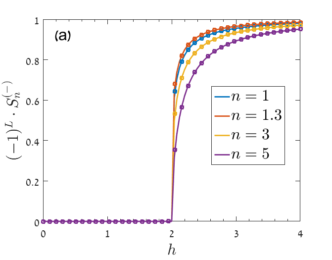
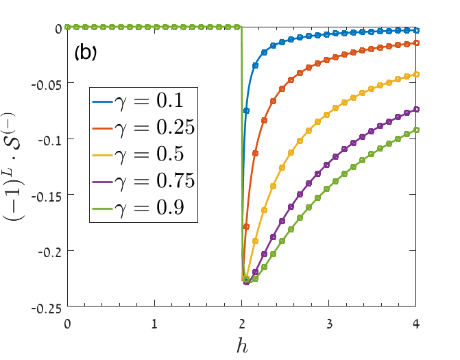
Figure 5: (a) $\left(-1\right)^{L}S_{n}^{\left(-\right)}$ in a subsystem of $L$ sites of a gapped XY chain, for anisotropy factor $\gamma=0.5$. The results were computed numerically for $L=200$ using (92) (dots) and analytically for $L\rightarrow\infty$ using (101) (continuous lines). (b) $\left(-1\right)^{L}\mathcal{S}^{\left(-\right)}$ in a subsystem of $L$ sites of a gapped XY chain, computed numerically for $L=200$ using (102) (dots) and analytically for $L\rightarrow\infty$ using (103) (continuous lines).

Fig. 5(a) shows a comparison between the asymptotic analytical result for $S_{n}^{\left(-\right)}$ and the numerical result. It indicates a very good agreement between the two calculations, and in particular confirms two conspicuous properties of the analytical result in the large $L$ limit: that $S_{n}^{\left(-\right)}\rightarrow 0$ in the $h<2$ regime, and that $\left|S_{n}^{\left(-\right)}\right|\rightarrow 1$ as $h\rightarrow\infty$. A numerical calculation of $S_{2}^{\left(-\right)}$ for several values of $L$ has previously appeared in [37].

We use our calculation of $S_{n}^{\left(-\right)}$ in order to calculate $\mathcal{S}^{\left(-\right)}=-\underset{n\rightarrow 1}{\lim}\partial_{n}S_{n}^{\left(-\right)}$ at the large $L$ limit. Relying on (92), we can obtain an explicit expression for $\mathcal{S}^{\left(-\right)}$:

$$\mathcal{S}^{\left(-\right)}=\left(-1\right)^{L}\underset{m=1}{\overset{L}{\sum}}\left(\underset{j\neq m}{\Pi}\nu_{j}\right)\cdot\left[\frac{1-\nu_{m}}{2}\ln\left(\frac{1-\nu_{m}}{2}\right)-\frac{1+\nu_{m}}{2}\ln\left(\frac{1+\nu_{m}}{2}\right)\right].$$ (102)

This expression can be used for numerical estimates of ${\cal S}^{\left(-\right)}$.

From (101) we can now calculate $\mathcal{S}^{\left(-\right)}$ as $L\rightarrow\infty$:

$$\underset{L\rightarrow\infty}{\lim}\left(-1\right)^{L}\mathcal{S}^{\left(-\right)}=\begin{cases}0,&h<2\\ \frac{\sqrt{k^{\prime}}}{3}\left[\ln 2-\frac{1}{2}\ln\left(k\cdot k^{\prime}\right)-\frac{I\left(k\right)I\left(k^{\prime}\right)}{\pi}\left(1+k^{2}\right)\right],&h>2\end{cases}.$$ (103)

The details of this calculation appear in subsection A.4 of the appendix. ${\cal S}^{\left(-\right)}$ is plotted in Fig. 5(b), where again good agreement between the analytical estimate and the numerical result is evident. Figs. 6(a)-(b) show the difference between the analytical limit for $L\rightarrow\infty$ and the numerical results for finite $L$. They demonstrate that away from the vicinity of $h=2$, where the phase transition occurs, corrections to the asymptotic result vanish rapidly as $L$ grows, and it is apparent that e.g. for $\gamma=0.5$ these corrections turn negligible even for a relatively short subsystem. As $h$ nears $h=2$, we need a larger value of $L$ in order for the deviation to be small.

Both $S_{n}^{\left(-\right)}$ and ${\cal S}^{\left(-\right)}$ illustrate a striking property of the phase in which the system is found for $h<2$: since $S_{n}^{\left(-\right)}={\cal S}^{\left(-\right)}=0$, we obtain that for $h<2$, the system satisfies $S_{n}^{\left(\mathrm{even}\right)}=S_{n}^{\left(\mathrm{odd}\right)}$ and ${\cal S}^{\left(\mathrm{even}\right)}={\cal S}^{\left(\mathrm{odd}\right)}$. This property stems from the fact that we can write the RDM as $\rho_{A}=\exp\left(-H_{A}\right)$ where the entanglement Hamiltonian $H_{A}$ is quadratic [38, 48], and treat $H_{A}$ as the Hamiltonian of an effective system of a 1D open fermionic chain with $L$ sites. $H_{A}$ is expected to have the same modes at the virtual edges of the subsystem as the original system (the Kitaev chain) would host at a physical edge [29]. Thus the phase $h<2$ corresponds to a topologically non-trivial phase of $H_{A}$ where two Majorana zero-modes — one at each end of the system — remain decoupled, provided that the virtual chain is long enough [53]. Combining these two Majorana operators yields a fermionic operator whose occupancy does not change the eigenvalues of $H_{A}$, and thus induces a two-fold degeneracy in the system: every eigenstate of $H_{A}$ with an even total fermionic number has a corresponding eigenstate with the same eignevalue but with an odd total fermionic number, and vice versa. This degeneracy persists as long as $h<2$. This explains why in the large $L$ limit, the contributions to the entropy from the block that corresponds to an even $Q_{A}$ and the block that corresponds to an odd $Q_{A}$ are exactly the same. Our work provides a rigorous proof of this behavior for the system considered. These observations allow us to explain the finite $L$ corrections to our results, which become noticeable for $L\lesssim 50$, as depicted in Figs. 6(a)-(b).

Since for $h\neq 2$ the system is gapped, the correlations vanish exponentially as $L\rightarrow\infty$ [54], and therefore so do the corrections to the limiting values of $S_{n}^{\left(-\right)}$ and $\mathcal{S}^{\left(-\right)}$. For $h<2$ the corrections are dominated by the hybridization of the entanglement Majorana edge-modes: though they are localized exponentially at the ends of the virtual chain [53], for finite $L$ the virtual edge Majorana fermions exhibit some overlap, and therefore a true degeneracy is not achieved [53] for most values of $h<2$, resulting in a finite nonzero value of the lowest eigenvalue $\left|\nu_{1}\right|\equiv\min\left|\nu_{m}\right|$. Yet for certain values of $h<2$ the virtual Majorana wave functions interfere destructively, and this creates the minima apparent in Figs. 6(a)-(d) in both $\left|\mathcal{S}^{\left(-\right)}\right|$ and $\left|\nu_{1}\right|$. This in fact suggests that the finite size corrections to $\mathcal{S}^{\left(-\right)}$ are dominated by $\nu_{1}$,

$$\left|{\cal S}^{\left(-\right)}\right|\approx\left|\frac{1-\nu_{1}}{2}\ln\left(\frac{1-\nu_{1}}{2}\right)-\frac{1+\nu_{1}}{2}\ln\left(\frac{1+\nu_{1}}{2}\right)\right|.$$ (104)

The accuracy of this relation can serve as a quantitative test for the above arguments. And indeed, calculating the ratio between this approximation and $\left|{\cal S}^{\left(-\right)}\right|$ for the cases that appear in Figs. 6(a)-(b), we get that for $h<1.9$ (outside the vicinity of the critical point $h=2$), the contribution of $\nu_{1}$ to ${\cal S}^{\left(-\right)}$ is always above $85\%$ for $\gamma=0.5$, and always above $65\%$ for $\gamma=0.1$.

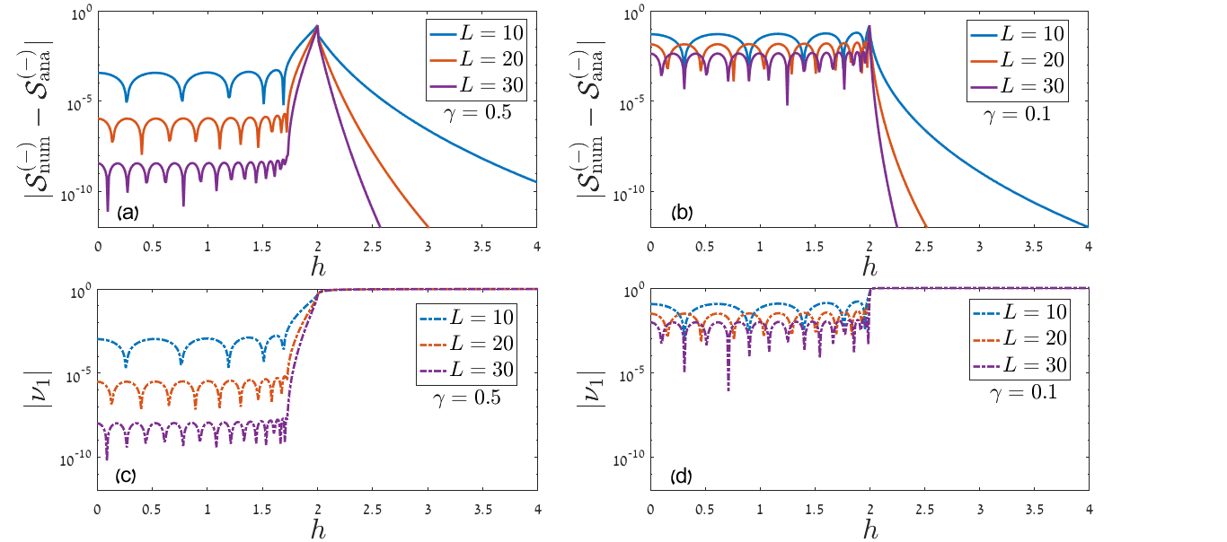
Figure 6: Upper panels: Absolute deviation of the analytical estimate (103) of $\mathcal{S}^{\left(-\right)}$ as $L\rightarrow\infty$ (denoted by $\mathcal{S}_{\mathrm{ana}}^{\left(-\right)}$) from the numerical estimate (102) for finite $L$ (denoted by $\mathcal{S}_{\mathrm{num}}^{\left(-\right)}$), for (a) $\gamma=0.5$ and (b) $\gamma=0.1$. Lower panels: $\left|\nu_{1}\right|$ as a function of the magnetic field, for (c) $\gamma=0.5$ and (d) $\gamma=0.1$. The minima that appear for $h<2$ in all of the graphs correspond to points where $\left|\nu_{1}\right|$ vanishes and therefore ${\cal S}_{\mathrm{num}}^{\left(-\right)}$ vanishes as well.

Considerations similar to those detailed above allow the extension of our main results (101) and (103) to $0>h\neq-2$. The limit $\underset{L\rightarrow\infty}{\lim}\left|S_{n}^{\left(-\right)}\right|$ is symmetric in $h$, and therefore, in particular, it tends to $1$ as $h\rightarrow-\infty$. However, the sign ambiguity is resolved in a different way than in the $h>0$ case: for finite $L$ we expect that in the $h\rightarrow-\infty$ limit, all sites of $A$ become unoccupied such that $Q_{A}=0$ with probability $1$. We thus obtain that as $h\rightarrow-\infty$, $S_{n}^{\left(-\right)}\rightarrow 1$ both for even and odd $L$, and so for $0>h\neq-2$ the limit $\underset{L\rightarrow\infty}{\lim}S_{n}^{\left(-\right)}$ exists and is also positive.

The extensions of (101) and (103) to $0>h\neq-2$ are therefore symmetric, apart from the absence of the $\left(-1\right)^{L}$ prefix, namely

$$\underset{L\rightarrow\infty}{\lim}S_{n}^{\left(-\right)}\Big{\rvert}_{h}=\underset{L\rightarrow\infty}{\lim}\left(-1\right)^{L}S_{n}^{\left(-\right)}\Big{\rvert}_{-h}\,\,\,\left(0>h\neq-2\right),$$ (105)

and

$$\underset{L\rightarrow\infty}{\lim}{\cal S}^{\left(-\right)}\Big{\rvert}_{h}=\underset{L\rightarrow\infty}{\lim}\left(-1\right)^{L}{\cal S}^{\left(-\right)}\Big{\rvert}_{-h}\,\,\,\left(0>h\neq-2\right).$$ (106)

5.2 Gapless XY model

Here we calculate the asymptotics of $S_{n}^{\left(\pm\right)}$ for the case where the system is gapless, i.e., $h=2$. Following [45] we write

$$\ln\left|S_{n}^{\left(\pm\right)}\right|=\mathrm{Re}\left\{\underset{\varepsilon,\delta\rightarrow 0^{+}}{\lim}\frac{1}{4\pi i}\underset{c\left(\varepsilon,\delta\right)}{\int}e_{n}^{\left(\pm\right)}\left(1+\varepsilon,\lambda\right)\frac{d}{d\lambda}\ln\tilde{D}_{L}\left(\lambda\right)d\lambda\right\},$$ (107)

where $c\left(\varepsilon,\delta\right)$ is the contour shown in Fig. 1(a), and

$$e_{n}^{\left(\pm\right)}\left(x,\nu\right)\equiv\ln\left[\left(\frac{x-\nu}{2}\right)^{n}\pm\left(\frac{x+\nu}{2}\right)^{n}\right].$$ (108)

Using the asymptotic approximation for $\tilde{D}_{L}\left(\lambda\right)$ in (46), we obtain that

$$\frac{d}{d\lambda}\ln\tilde{D}_{L}\left(\lambda\right)\sim\left(\frac{1}{\lambda+1}+\frac{1}{\lambda-1}\right)L-\frac{4i}{\pi}\cdot\frac{\beta\left(\lambda\right)}{\left(\lambda+1\right)\left(\lambda-1\right)}\ln L.$$ (109)

This expression is reminiscent of (50) from the calculation of the REE in the gapless XX model, and we can therefore carry out the integration along the same lines of argument, so that eventually we get

$$\ln\left|S_{n}^{\left(\pm\right)}\right|\sim\left[\frac{1}{12}\left(\frac{1}{n}-n\right)-\frac{\eta_{\pm}}{4n}\right]\ln L,$$ (110)

where $\eta_{+}=0$ and $\eta_{-}=1$. Since $S_{n}^{\left(+\right)}=\left|S_{n}^{\left(+\right)}\right|$, we have in particular obtained that for the gapless XY model

$$\ln S_{n}^{\left(+\right)}\sim\frac{1}{12}\left(\frac{1}{n}-n\right)\ln L,$$ (111)

a special case of a result which was derived and verified numerically in [50]. The coefficient of the logarithm is halved as compared to (53) with $\alpha=0$, since a Majorana mode rather than a complex fermion is gapless here, in accordance with CFT predictions [4].

$S_{n}^{\left(-\right)}$ is again determined only up to a sign,

$$\left|S_{n}^{\left(-\right)}\right|\approx A\left(n,\gamma\right)L^{-\frac{1}{6n}-\frac{n}{12}},$$ (112)

where $A\left(n,\gamma\right)$ is some positive factor independent of $L$, assuming that the largest subleading contribution not appearing in the approximation (46) does not depend on $L$. We have verified this assumption numerically by fitting to the results a function of $L$ that scales as $L^{-1/6n-n/12}$, while the proportionality constant remained a free parameter. An example is shown in Fig. 7(a), where good agreement between numerical and analytical results is evident. Lead by similar considerations as in the case of the gapped XY model, we can determine the sign of $S_{n}^{\left(-\right)}$ to be $\left(-1\right)^{L}$, so that

$$\left(-1\right)^{L}S_{n}^{\left(-\right)}\approx A\left(n,\gamma\right)L^{-\frac{1}{6n}-\frac{n}{12}}.$$ (113)

Specific attributes of the factor $A\left(n,\gamma\right)$ are generally not captured by known theorems or conjectures we are aware of, and its analysis is beyond the scope of this work. We show its typical behavior, as extracted from numerical results, in Fig. 7(b). The result (113) confirms a previous prediction based on CFT considerations [20].

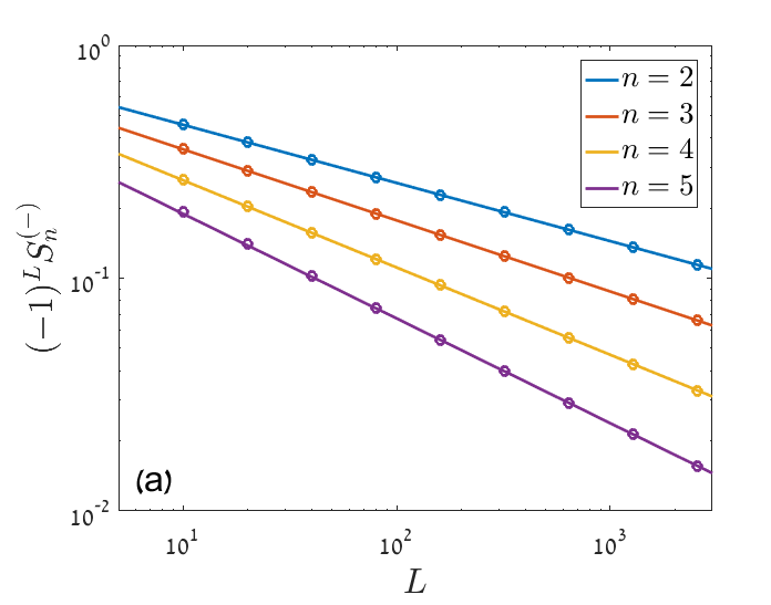
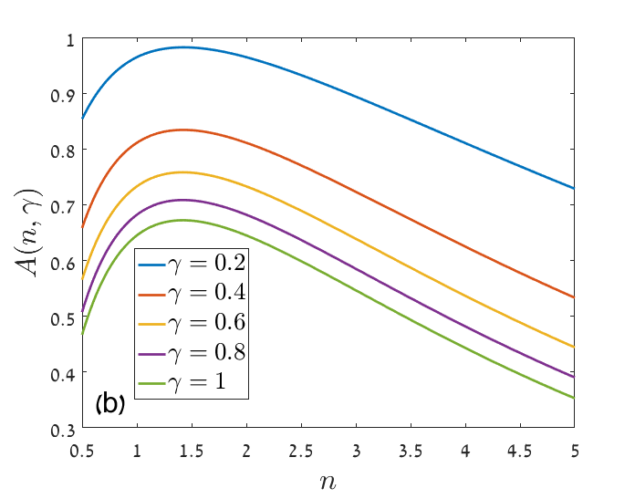
Figure 7: (a) $\left(-1\right)^{L}S_{n}^{\left(-\right)}$ in a subsystem of $L$ sites of a gapless XY chain ($h=2)$, for anisotropy factor $\gamma=0.4$. The results were computed numerically using (92) (dots) and analytically using (113) (continuous lines). For the analytical results, the unknown factor $A\left(n,\gamma\right)$ was extracted from a fit to the numerical results. (b) The factor $A\left(n,\gamma\right)$ for several values of anisotropy factor $\gamma$, as extracted from fits to numerical results.

The parity-resolved vNEE $\mathcal{S}^{\left(-\right)}$ for $h=2$ is therefore

$$\left(-1\right)^{L}\mathcal{S}^{\left(-\right)}\approx-\frac{A\left(1,\gamma\right)}{12}L^{-\frac{1}{4}}\ln L.$$ (114)

As before, we can extend the results for $S_{n}^{\left(-\right)}$ and $\mathcal{S}^{\left(-\right)}$ to $h=-2$ by simply omitting the $\left(-1\right)^{L}$ prefix.

6 Generalization to higher dimensions

In order to find the leading asymptotic behavior of the charged-resolved REE in a $d$-dimensional gapless free Fermi gas, we rely in this section on a formula conjectured by Widom [40] and proven for several particular cases [55, 56, 57]. A result similar to that which we are about to present was derived in a recent work [22], which discussed a different but related quantity, the accessible EE defined there.

Let us describe the physical scale of subsystem $A$ in terms of a typical linear dimension $L\gg 1$ (made dimensionless by e.g. normalizing by the lattice constant), so that $A$ contains $L^{d}$ sites. We denote by $\Omega_{A}$ the bounded region in real space that is occupied by $A$, and by $\Gamma$ the region in momentum space that is occupied by the Fermi sea. We further denote by $P$ and $Q$ the operators which represent projections into $\Gamma$ and $\Omega_{A}$, respectively. Following [20], we can write

$$\ln S_{n}\left(\alpha\right)=\mathrm{Tr}\ln\left[C^{n}e^{i\alpha}+\left(1-C\right)^{n}\right],$$ (115)

where $C_{ij}=\langle a_{i}^{\dagger}a_{j}\rangle$ ($i,j=1,\ldots,L^{d}$) is the fermionic correlation matrix, restricted to subsystem $A$. In the ground state $C=QPQ$, and therefore $\ln S_{n}\left(\alpha\right)=\mathrm{Tr}f_{n,\alpha}\left(QPQ\right)$, where $f_{n,\alpha}\left(t\right)=\ln\left[t^{n}e^{i\alpha}+\left(1-t\right)^{n}\right]$.

We now introduce the notations

$$c_{1}=\frac{1}{\left(2\pi\right)^{d}L^{d}}\underset{\Omega_{A}}{\int}\underset{\Gamma}{\int}\text{d}\boldsymbol{x}\text{d}\boldsymbol{p}\,\,\,\text{and}\,\,\,c_{2}=\frac{1}{\left(2\pi\right)^{d+1}L^{d-1}}\underset{\partial\Omega_{A}}{\int}\underset{\partial\Gamma}{\int}\left|\boldsymbol{n_{x}}\cdot\boldsymbol{n_{p}}\right|\text{d}S_{x}\text{d}S_{p},$$ (116)

where $\boldsymbol{n_{x}},\boldsymbol{n_{p}}$ are unit vectors that are normal to $\partial\Omega_{A},\partial\Gamma$, respectively, and the units of $\boldsymbol{x}$ are set by the lattice constant such that the volume of a lattice unit cell equals unity. The normalization by powers of $L$ was chosen so that the scaling with $L$ of the final results becomes apparent. Note that in previous works [22, 56, 58, 59] this was achieved by a different convention of measuring $\boldsymbol{x}$ in units of $L$. A function $f$ is said to obey the Widom formula [56, 58, 59] if for $L\gg 1$,

$$\mathrm{Tr}f\left(QPQ\right)=c_{1}f\left(1\right)L^{d}+c_{2}U\left(f\right)L^{d-1}\ln L+o\left(L^{d-1}\ln L\right),$$ (117)

where we have defined

$$U\left(f\right)\equiv\underset{0}{\overset{1}{\int}}\frac{f\left(t\right)-tf\left(1\right)}{t\left(1-t\right)}dt.$$ (118)

Note that the formula (117) was proven rigorously only for regions $\Omega_{A}$, $\Gamma$ which satisfy certain regularity conditions, detailed in [56].

In [56] it was shown that $f:\mathbb{R}\rightarrow\mathbb{R}$ satisfies the Widom formula in two specific cases:

• $f$ is infinitely differentiable and $f\left(0\right)=0$.

• $f$ is infinitely differentiable on $\mathbb{R}\setminus\left\{0,1\right\}$ and there exist real constants $K,\beta>0$ so that for every $t\in\left[0,1\right]$, $\left|f\left(t\right)\right|\leq Kt^{\beta}\left(1-t\right)^{\beta}$.

Let us define $F_{n,\alpha}\left(t\right)=f_{n,\alpha}\left(t\right)-f_{n,\alpha}\left(1\right)t$ for every $n>0$ and $-\pi<\alpha<\pi$. Both the real and the imaginary parts of $F_{n,\alpha}$ satisfy the requirements of Case (b) with $\beta=\min\left\{n,1\right\}$, and we can therefore apply the Widom formula (117) to $F_{n,\alpha}$. Using the fact that $F_{n,\alpha}\left(1\right)=0$ and $U\left(F_{n,\alpha}\right)=U\left(f_{n,\alpha}\right)$, we obtain that

$$\mathrm{Tr}F_{n,\alpha}\left(QPQ\right)=c_{2}U\left(f_{n,\alpha}\right)L^{d-1}\ln L+o\left(L^{d-1}\ln L\right).$$ (119)

The LHS of the last equality can be written as $\mathrm{Tr}F_{n,\alpha}\left(QPQ\right)=\mathrm{Tr}f_{n,\alpha}\left(QPQ\right)-f_{n,\alpha}\left(1\right)\mathrm{Tr}g\left(QPQ\right)$, where $g\left(t\right)=t$. $g$ obeys the Widom formula because it fulfills the requirements of Case (a), so by applying the Widom formula to $\mathrm{Tr}g\left(QPQ\right)$ as well we can thus conclude that

$$\mathrm{Tr}f_{n,\alpha}\left(QPQ\right)=\mathrm{Tr}F_{n,\alpha}\left(QPQ\right)+f_{n,\alpha}\left(1\right)\mathrm{Tr}g\left(QPQ\right)=c_{1}f_{n,\alpha}\left(1\right)L^{d}+c_{2}U\left(f_{n,\alpha}\right)L^{d-1}\ln L+o\left(L^{d-1}\ln L\right),$$ (120)

which shows that $f_{n,\alpha}$ itself obeys the Widom formula.

Consequently, we have for every $-\pi<\alpha<\pi$

$$\ln S_{n}\left(\alpha\right)=ic_{1}L^{d}\alpha+c_{2}U\left(f_{n,\alpha}\right)L^{d-1}\ln L+o\left(L^{d-1}\ln L\right).$$ (121)

Substituting $f_{n,\alpha}$ into (118) and using the change of variables $u=\ln\frac{t}{1-t}$, we get

$$U\left(f_{n,\alpha}\right)=\underset{-\infty}{\overset{\infty}{\int}}\left[\ln\left(\frac{1+e^{nu+i\alpha}}{\left(1+e^{u}\right)^{n}}\right)-\frac{i\alpha}{1+e^{-u}}\right]du=\frac{\pi^{2}}{6}\left(\frac{1}{n}-n\right)-\frac{\alpha^{2}}{2n}.$$ (122)

We can therefore write

$$S_{n}\left(\alpha\right)\approx\exp\left[ic_{1}L^{d}\alpha-\frac{1}{2}\cdot\frac{c_{2}L^{d-1}\ln L}{n}\alpha^{2}+\frac{\pi^{2}}{6}\left(\frac{1}{n}-n\right)c_{2}L^{d-1}\ln L\right],$$ (123)

and finally conclude from (8) that in $d$ dimensions, the charge-resolved REE satisfies

$$S_{n}\left(Q_{A}\right)\approx\sqrt{\frac{n}{2\pi c_{2}L^{d-1}\ln L}}\exp\left[\frac{-n\left(Q_{A}-c_{1}L^{d}\right)^{2}}{2c_{2}L^{d-1}\ln L}+\frac{\pi^{2}}{6}\left(\frac{1}{n}-n\right)c_{2}L^{d-1}\ln L\right].$$ (124)

For $d=1$, $c_{1}L^{d}=\langle Q_{A}\rangle$ and $c_{2}L^{d-1}=1/\pi^{2}$, and therefore

$$S_{n}\left(Q_{A}\right)\approx S_{n}\cdot\sqrt{\frac{\pi n}{2\ln L}}\exp\left[\frac{-n\pi^{2}\left(Q_{A}-\langle Q_{A}\rangle\right)^{2}}{2\ln L}\right]\,\,\,\left(d=1\right),$$ (125)

which is in complete agreement with the approximation (58) to leading order in $\ln L/n$.

7 Conclusions and future outlook

In this work we have obtained analytically the asymptotic behavior of the flux-resolved REE in a 1D spin (fermion) chain, both for a gapless XX (tight binding) chain and for the XY (Kitaev) chain, as well as in higher dimensions. In 1D, these analytical results have been shown in general to be in very good agreement with numerical results, even for a subsystem of moderate length.

For the gapless XX model our results agree with previous CFT arguments, and extend them beyond leading order in $\mathcal{L}$. While the Gaussian approximation and the leading order approximation of $S_{n}\left(\alpha\right)$ deviate considerably from numerical results, the approximation that includes all terms up to order ${\cal O}\left({\cal L}^{-1}\right)$ has been extremely accurate in the cases we have examined. We were also able to provide a meaning to the corrections beyond the leading order approximation, by showing that they arise from a periodic structure, in line with CFT arguments. In higher dimensions, we derived an approximated expression for the symmetry-resolved REE in a gapless gas of free fermions. Under such an approximation the symmetry-resolved EE is proportionate to a Gaussian distribution of the charge, akin to the equipartition property noted in [21].

For the gapped XY model, our results provide a way to obtain analytical expressions for the parity-resolved decomposition of both the REE and the vNEE. These expressions are, on the face of it, limiting expressions that apply to a subsystem of infinite length, but our calculations have shown that they match the numerical results even for relatively short subsystems, due to the exponential decay of the correlations. We have also detected a topologically non-trivial phase in the virtual chain described by the entanglement Hamiltonian, which explains why for $|h|<2$ there is an equal contribution to the EE from states where $Q_{A}$ is odd and states where $Q_{A}$ is even. At the critical points, $h=\pm 2$, we have found a power-law behavior matching previous CFT predictions [20].

The use of the generalized Fisher-Hartwig (or, in higher dimensions, the Widom) conjecture was thus proven to be a powerful method for producing accurate estimates of symmetry-resolved EE. This suggests several prospects of future research, applying similar methods of calculation to questions such as the symmetry-resolved EE in topological systems [37, 60, 61], or in systems out of equilibrium, for example following a quench [62]. Another possible direction of research is the study of the symmetry-resolved EE of a bipartition into disconnected subsystems [63].

Note added: When this work was close to completion a related work appeared online [64] which employs Fisher-Hartwig techniques to calculate the resolved entropy of the XX chain to order $\mathcal{O}\left(\mathcal{L}^{0}\right)$. Our results go further in (i) performing the XX calculations to order $\mathcal{O}\left(\mathcal{L}^{-1}\right)$, which is especially important in the vicinity of $\alpha=\pm\pi$; (ii) studying the XY (Kitaev) case; (iii) treating higher-dimensional gapless fermionic systems.

Appendix A Appendix: Details of the calculations

A.1 Asymptotics of the correlation matrix determinant (gapless XY model)

We derive here the leading order asymptotic approximation for the determinant $\tilde{D}_{L}\left(\lambda\right)$ defined in (43), for the case of a gapless XY chain ($h=2$). A generalized version of the Fisher-Hartwig formula was conjectured in [50, 51], regarding the determinant of a block Toeplitz matrix of the form

$$T_{L}\left[\mathcal{M}\right]=\left(\begin{array}[]{cccc}\tilde{\Pi}_{0}&\tilde{\Pi}_{-1}&\cdots&\tilde{\Pi}_{1-L}\\ \tilde{\Pi}_{1}&\tilde{\Pi}_{0}&&\vdots\\ \vdots&&\ddots&\vdots\\ \tilde{\Pi}_{L-1}&\cdots&\cdots&\tilde{\Pi}_{0}\end{array}\right),\,\,\,\tilde{\Pi}_{m}\equiv\frac{1}{2\pi}\underset{0}{\overset{2\pi}{\int}}d\theta e^{-im\theta}\mathcal{M}\left(\theta\right),$$ (A.1)

where $\mathcal{M}\left(\theta\right)$ is a piecewise continuous $d\times d$ matrix with jump discontinuities at the points $\theta_{r}$, $r=0,\ldots,R$. We define for each discontinuity $\mathcal{M}_{r}^{\pm}\equiv\underset{\theta\rightarrow\theta_{r}^{\pm}}{\lim}\mathcal{M}\left(\theta\right)$, and assume that for each $r$, $\mathcal{M}_{r}^{+}$ and $\mathcal{M}_{r}^{-}$ commute. This allows us to find a joint diagonalizing basis for $\mathcal{M}_{r}^{\pm}$, and we denote the corresponding eigenvalues by $\mu_{r,j}^{\pm}$, $j=1,\ldots,d$. According to the conjecture [51], for the first two leading terms of the large $L$ approximation of $\ln\det T_{L}\left[\mathcal{M}\right]$ we then have

$$\ln\det T_{L}\left[\mathcal{M}\right]=\frac{L}{2\pi}\underset{0}{\overset{2\pi}{\int}}d\theta\ln\left(\det\mathcal{M}\left(\theta\right)\right)+\frac{\ln L}{4\pi^{2}}\underset{r=0}{\overset{R}{\sum}}\underset{j=1}{\overset{d}{\sum}}\left(\ln\left(\frac{\mu_{r,j}^{-}}{\mu_{r,j}^{+}}\right)\right)^{2}+\cdots.$$ (A.2)

For $h=2$, $\tilde{D}_{L}\left(\lambda\right)$ is of the form described above, i.e., $\tilde{D}_{L}\left(\lambda\right)=\det T_{L}\left[\mathcal{M}\right]$ for $\mathcal{M}\left(\theta\right)=i\lambda I_{2}-\mathcal{G}\left(\theta\right)$. Now $\mathcal{M}$ has a single discontinuity at $\theta_{0}=0$, with

$$\mathcal{M}_{0}^{\pm}=\left(\begin{array}[]{cc}i\lambda&\pm i\\ \pm i&i\lambda\end{array}\right),$$ (A.3)

from which we obtain that $\mu_{0,1}^{\pm}=i\lambda\pm i$ and $\mu_{0,2}^{\pm}=i\lambda\mp i$. Since $\det\mathcal{M}\left(\theta\right)=1-\lambda^{2}$ is independent of $\theta$, we finally arrive at

$$\ln\tilde{D}_{L}\left(\lambda\right)=\ln\left(1-\lambda^{2}\right)L-2\beta^{2}\left(\lambda\right)\ln L+\cdots.$$ (A.4)

A.2 Leading order approximation of the flux-resolved REE (XX model)

From the Fisher-Hartwig conjecture we have derived the leading order approximation for the asymptotic expression for $S_{n}\left(\alpha\right)$:

$$\ln S_{n}^{\left(0\right)}\left(\alpha\right) =i\frac{\alpha}{2}L+\underset{\varepsilon,\delta\rightarrow 0^{+}}{\lim}\frac{1}{2\pi i}\underset{c\left(\varepsilon,\delta\right)}{\int}e_{n}^{\left(\alpha\right)}\left(1+\varepsilon,\lambda\right)\left(\frac{k_{F}/\pi}{\lambda-1}+\frac{1-k_{F}/\pi}{\lambda+1}\right)Ld\lambda+$$

$$+\underset{\varepsilon,\delta\rightarrow 0^{+}}{\lim}\frac{1}{2\pi i}\underset{c\left(\varepsilon,\delta\right)}{\int}e_{n}^{\left(\alpha\right)}\left(1+\varepsilon,\lambda\right)\left(-\frac{4i}{\pi}\cdot\frac{\beta\left(\lambda\right)}{\left(\lambda+1\right)\left(\lambda-1\right)}\left[\ln\mathcal{L}+\left(1+\gamma_{E}\right)+\Upsilon\left(\lambda\right)\right]\right)d\lambda.$$ (A.5)

Regarding the first integral, it is easily shown that

$$\underset{\varepsilon,\delta\rightarrow 0^{+}}{\lim}\frac{1}{2\pi i}\underset{c\left(\varepsilon,\delta\right)}{\int}e_{n}^{\left(\alpha\right)}\left(1+\varepsilon,\lambda\right)\left(\frac{k_{F}/\pi}{\lambda-1}+\frac{1-k_{F}/\pi}{\lambda+1}\right)Ld\lambda=i\left(-1+\frac{2k_{F}}{\pi}\right)\frac{\alpha}{2}L.$$ (A.6)

As for the second integral, we use the fact that for every $-1<x<1$,

$$\beta\left(x+i0^{\pm}\right)=-iW\left(x\right)\mp\frac{1}{2},$$ (A.7)

where $W\left(x\right)\equiv\frac{1}{2\pi}\ln\frac{1+x}{1-x}$. It can be shown that the contribution from the circular arcs of the contour $c\left(\varepsilon,\delta\right)$ vanishes as $\varepsilon,\delta\rightarrow 0^{+},$ and therefore we get

$$\underset{\varepsilon,\delta\rightarrow 0^{+}}{\lim}\frac{1}{2\pi i}\underset{c\left(\varepsilon,\delta\right)}{\int}e_{n}^{\left(\alpha\right)}\left(1+\varepsilon,\lambda\right)\left(-\frac{4i}{\pi}\cdot\frac{\beta\left(\lambda\right)}{\left(\lambda+1\right)\left(\lambda-1\right)}\left[\ln\mathcal{L}+\left(1+\gamma_{E}\right)+\Upsilon\left(\lambda\right)\right]\right)d\lambda=$$

$$=\frac{\left(\ln\mathcal{L}+\left(1+\gamma_{E}\right)\right)}{\pi^{2}}\underset{\varepsilon\rightarrow 0^{+}}{\lim}\underset{-1+\frac{\varepsilon}{2}}{\overset{1-\frac{\varepsilon}{2}}{\int}}\frac{2e_{n}^{\left(\alpha\right)}\left(1+\varepsilon,x\right)}{1-x^{2}}dx+$$

$$+\underset{\varepsilon\rightarrow 0^{+}}{\lim}\underset{k=1}{\overset{\infty}{\sum}}\frac{1}{\pi^{2}k}\underset{-1+\frac{\varepsilon}{2}}{\overset{1-\frac{\varepsilon}{2}}{\int}}\left[\frac{\left(\frac{1}{2}-iW\left(x\right)\right)^{3}}{k^{2}-\left(\frac{1}{2}-iW\left(x\right)\right)^{2}}+\frac{\left(\frac{1}{2}+iW\left(x\right)\right)^{3}}{k^{2}-\left(\frac{1}{2}+iW\left(x\right)\right)^{2}}\right]\frac{2e_{n}^{\left(\alpha\right)}\left(1+\varepsilon,x\right)}{1-x^{2}}dx=$$

$$=\frac{\ln\mathcal{L}}{\pi^{2}}\underset{\varepsilon\rightarrow 0^{+}}{\lim}\underset{-1+\frac{\varepsilon}{2}}{\overset{1-\frac{\varepsilon}{2}}{\int}}\frac{2e_{n}^{\left(\alpha\right)}\left(1+\varepsilon,x\right)}{1-x^{2}}dx-\frac{1}{\pi^{2}}\underset{\varepsilon\rightarrow 0^{+}}{\lim}\underset{-1+\frac{\varepsilon}{2}}{\overset{1-\frac{\varepsilon}{2}}{\int}}\left[\psi\left(\frac{1}{2}+iW\left(x\right)\right)+\psi\left(\frac{1}{2}-iW\left(x\right)\right)\right]\frac{e_{n}^{\left(\alpha\right)}\left(1+\varepsilon,x\right)}{1-x^{2}}dx.$$ (A.8)

Here we denoted by $\psi\left(x\right)$ the Digamma function, $\psi\left(x\right)=\frac{\Gamma^{\prime}\left(x\right)}{\Gamma\left(x\right)}$, and used the identity [44]

$$\underset{k=1}{\overset{\infty}{\sum}}\frac{1}{k}\left[\frac{\left(\frac{1}{2}+iw\right)^{3}}{k^{2}-\left(\frac{1}{2}+iw\right)^{2}}+\frac{\left(\frac{1}{2}-iw\right)^{3}}{k^{2}-\left(\frac{1}{2}-iw\right)^{2}}\right]=-1-\gamma_{E}-\frac{1}{2}\left[\psi\left(\frac{1}{2}+iw\right)+\psi\left(\frac{1}{2}-iw\right)\right].$$ (A.9)

Using a change of variables $u=\ln\frac{1+x}{1-x}$, and taking the limit $\varepsilon\rightarrow 0^{+}$, we have

$$\underset{\varepsilon\rightarrow 0^{+}}{\lim}\underset{-1+\frac{\varepsilon}{2}}{\overset{1-\frac{\varepsilon}{2}}{\int}}\frac{2e_{n}^{\left(\alpha\right)}\left(1+\varepsilon,x\right)}{1-x^{2}}dx =-n\underset{-\infty}{\overset{\infty}{\int}}\frac{u}{e^{u}+1}\cdot\frac{e^{nu+i\frac{\alpha}{2}}-e^{u-i\frac{\alpha}{2}}}{e^{nu+i\frac{\alpha}{2}}+e^{-i\frac{\alpha}{2}}}du=$$

$$=-\frac{\pi^{2}}{6}n+\frac{2}{n}\underset{k=1}{\overset{\infty}{\sum}}\frac{\left(-1\right)^{k+1}}{k^{2}}\cos\left(\alpha k\right).$$ (A.10)

Recalling the Fourier series of $\alpha^{2}$ in $\left(-\pi,\pi\right)$, we can now write for every $-\pi<\alpha<\pi$

$$\frac{\ln\mathcal{L}}{\pi^{2}}\underset{\varepsilon\rightarrow 0^{+}}{\lim}\underset{-1+\frac{\varepsilon}{2}}{\overset{1-\frac{\varepsilon}{2}}{\int}}\frac{2e_{n}^{\left(\alpha\right)}\left(1+\varepsilon,x\right)}{1-x^{2}}dx=\left[\frac{1}{6}\left(\frac{1}{n}-n\right)-\frac{\alpha^{2}}{2\pi^{2}n}\right]\ln\mathcal{L}.$$ (A.11)

Changing variables and taking the limit $\varepsilon\rightarrow 0^{+}$ as before, the second part of the integral turns out to be

$$-\frac{1}{\pi^{2}}\underset{\varepsilon\rightarrow 0^{+}}{\lim}\underset{-1+\frac{\varepsilon}{2}}{\overset{1-\frac{\varepsilon}{2}}{\int}}\left[\psi\left(\frac{1}{2}+iW\left(x\right)\right)+\psi\left(\frac{1}{2}-iW\left(x\right)\right)\right]\frac{e_{n}^{\left(\alpha\right)}\left(1+\varepsilon,x\right)}{1-x^{2}}dx=$$

$$=-\frac{i}{\pi}\underset{-\infty}{\overset{\infty}{\int}}\ln\left[\frac{2\cosh\left(\frac{nu}{2}+i\frac{\alpha}{2}\right)}{\left(2\cosh\left(\frac{u}{2}\right)\right)^{n}}\right]\frac{d}{du}\ln\frac{\Gamma\left(\frac{1}{2}+\frac{u}{2\pi i}\right)}{\Gamma\left(\frac{1}{2}-\frac{u}{2\pi i}\right)}du=$$

$$=-\frac{1}{\pi^{2}}\underset{0}{\overset{\infty}{\int}}\ln\left[\frac{2\cos\alpha+2\cosh\left(nu\right)}{\left(2\cosh\left(\frac{u}{2}\right)\right)^{2n}}\right]du\underset{0}{\overset{\infty}{\int}}\left[\frac{e^{-t}}{t}-\frac{\cos\left(\frac{ut}{2\pi}\right)}{2\sinh\left(\frac{t}{2}\right)}\right]dt.$$ (A.12)

Finally, we arrive at

$$\ln S_{n}^{\left(0\right)}\left(\alpha\right)=i\frac{k_{F}}{\pi}\alpha L+\left[\frac{1}{6}\left(\frac{1}{n}-n\right)-\frac{\alpha^{2}}{2\pi^{2}n}\right]\ln\mathcal{L}+\Upsilon_{0}\left(n,\alpha\right),$$

where

$$\Upsilon_{0}\left(n,\alpha\right)\equiv-\frac{1}{\pi^{2}}\underset{0}{\overset{\infty}{\int}}\ln\left[\frac{2\cos\alpha+2\cosh\left(nu\right)}{\left(2\cosh\left(\frac{u}{2}\right)\right)^{2n}}\right]du\underset{0}{\overset{\infty}{\int}}\left[\frac{e^{-t}}{t}-\frac{\cos\left(\frac{ut}{2\pi}\right)}{2\sinh\left(\frac{t}{2}\right)}\right]dt.$$ (A.13)

A.3 Gaussian approximation of the charge distribution (XX model)

We write

$$\Upsilon_{0}\left(n,\alpha\right)=-\frac{1}{\pi^{2}}\underset{0}{\overset{\infty}{\int}}\ln\left[\frac{2\cos\alpha+2\cosh\left(nu\right)}{\left(2\cosh\left(\frac{u}{2}\right)\right)^{2n}}\right]du\underset{0}{\overset{\infty}{\int}}\left[\frac{e^{-t}}{t}-\frac{\cos\left(\frac{ut}{2\pi}\right)}{2\sinh\left(\frac{t}{2}\right)}\right]dt=c_{0}\left(n\right)+c_{2}\left(n\right)\alpha^{2}+\mathcal{O}\left(\alpha^{4}\right),$$ (A.14)

and prove that $c_{2}\left(1\right)=-\frac{1+\gamma_{E}}{2\pi^{2}}$. Indeed, substituting $n=1$,

$$\ln\left[\frac{2\cos\alpha+2\cosh\left(u\right)}{\left(2\cosh\left(\frac{u}{2}\right)\right)^{2}}\right]=\ln\left[\frac{2+2\cosh\left(u\right)}{\left(2\cosh\left(\frac{u}{2}\right)\right)^{2}}\right]-\frac{1}{4\cosh^{2}\left(\frac{u}{2}\right)}\alpha^{2}+\mathcal{O}\left(\alpha^{4}\right),$$ (A.15)

and so

$$c_{2}\left(1\right)=\frac{1}{4\pi^{2}}\underset{0}{\overset{\infty}{\int}}\frac{1}{\cosh^{2}\left(\frac{u}{2}\right)}du\underset{0}{\overset{\infty}{\int}}\left[\frac{e^{-t}}{t}-\frac{\cos\left(\frac{ut}{2\pi}\right)}{2\sinh\left(\frac{t}{2}\right)}\right]dt.$$ (A.16)

We use

$$\underset{0}{\overset{\infty}{\int}}\frac{\cos\left(\frac{ut}{2\pi}\right)}{\cosh^{2}\left(\frac{u}{2}\right)}du=\underset{-\infty}{\overset{\infty}{\int}}\frac{e^{i\frac{t}{\pi}x}}{\cosh^{2}\left(x\right)}dx,$$ (A.17)

where the complex integral can be calculated using a rectangular contour with infinite horizontal sides at $\Im z=0$ and $\Im z=i\pi$, so that we get

$$\underset{0}{\overset{\infty}{\int}}\frac{\cos\left(\frac{ut}{2\pi}\right)}{\cosh^{2}\left(\frac{u}{2}\right)}du=\frac{2te^{-\frac{t}{2}}}{1-e^{-t}}.$$ (A.18)

We can therefore write

$$c_{2}\left(1\right) =\frac{1}{2\pi^{2}}\underset{0}{\overset{\infty}{\int}}\left[\frac{e^{-t}}{t}-\frac{te^{-\frac{t}{2}}}{\left(1-e^{-t}\right)\left(e^{\frac{t}{2}}-e^{-\frac{t}{2}}\right)}\right]dt=$$

$$=\frac{1}{2\pi^{2}}\underset{0}{\overset{\infty}{\int}}\left[\frac{1-e^{-t}-t}{t\left(e^{t}-1\right)}+\frac{1}{e^{t}-1}-\frac{te^{t}}{\left(e^{t}-1\right)^{2}}\right]dt=$$

$$=\frac{-\gamma_{E}}{2\pi^{2}}+\frac{1}{2\pi^{2}}\underset{0}{\overset{\infty}{\int}}\frac{d}{dt}\left(\frac{t}{e^{t}-1}\right)dt=$$

$$=-\frac{\gamma_{E}+1}{2\pi^{2}},$$ (A.19)

where we have used the identity $\gamma_{E}=\underset{0}{\overset{\infty}{\int}}\frac{e^{-t}+t-1}{t\left(e^{t}-1\right)}dt$ [49].

A.4 Decomposition of the vNEE (gapped XY model)

We present here a detailed calculation of $\mathcal{S}^{\left(-\right)}=-\underset{n\rightarrow 1}{\lim}\partial_{n}S_{n}^{\left(-\right)}$ as $L\rightarrow\infty$, based on the result for $S_{n}^{\left(-\right)}$ in (101). For $h<2$ we obviously have ${\cal S}^{\left(-\right)}\rightarrow 0$. For $h>2$, we can calculate the derivative of the expression for $S_{n}^{\left(-\right)}$ by rewriting it in terms of the Jacobi theta functions:

$$\left(-1\right)^{L}S_{n}^{\left(-\right)}\rightarrow\left[\frac{\left(kk^{\prime}\right)^{2n}k_{n}^{\prime 4}}{16^{n-1}k_{n}^{2}}\right]^{\frac{1}{12}}=\left[\frac{\theta_{2}^{4n}\left(q\right)\theta_{4}^{4n}\left(q\right)\theta_{4}^{8}\left(q^{n}\right)}{16^{n-1}\theta_{3}^{8n}\left(q\right)\theta_{2}^{4}\left(q^{n}\right)\theta_{3}^{4}\left(q^{n}\right)}\right]^{\frac{1}{12}}.$$ (A.20)

After some elementary steps, we arrive at

$$\left(-1\right)^{L}\mathcal{S}^{\left(-\right)}\rightarrow\frac{\sqrt{k^{\prime}}}{3}\left[\ln 2-\frac{1}{2}\ln\left(k\cdot k^{\prime}\right)+q\ln q\cdot\left(\frac{\theta_{3}^{\prime}\left(q\right)}{\theta_{3}\left(q\right)}+\frac{\theta_{2}^{\prime}\left(q\right)}{\theta_{2}\left(q\right)}-\frac{2\theta_{4}^{\prime}\left(q\right)}{\theta_{4}\left(q\right)}\right)\right],$$ (A.21)

where $\theta_{j}^{\prime}\left(q\right)\equiv\frac{d}{dq}\theta_{j}\left(q\right)$. For further simplification, we use the fact that

$$\frac{\theta_{3}^{\prime}\left(q\right)}{\theta_{3}\left(q\right)}+\frac{\theta_{2}^{\prime}\left(q\right)}{\theta_{2}\left(q\right)}-\frac{2\theta_{4}^{\prime}\left(q\right)}{\theta_{4}\left(q\right)}=\frac{d}{dq}\ln\left(\frac{\theta_{2}\theta_{3}}{\theta_{4}^{2}}\right)=\frac{d}{dq}\ln\left(\frac{k^{\frac{1}{2}}}{k^{\prime}}\right),$$ (A.22)

along with the identity [49]

$$\frac{k^{\frac{1}{2}}}{k^{\prime}}=2q^{\frac{1}{4}}\underset{m=1}{\overset{\infty}{\Pi}}\left(1+q^{m}\right)^{6},$$ (A.23)

in order to obtain that

$$q\left(\frac{\theta_{3}^{\prime}\left(q\right)}{\theta_{3}\left(q\right)}+\frac{\theta_{2}^{\prime}\left(q\right)}{\theta_{2}\left(q\right)}-\frac{2\theta_{4}^{\prime}\left(q\right)}{\theta_{4}\left(q\right)}\right)=\frac{1}{4}+6\underset{m=1}{\overset{\infty}{\sum}}\frac{mq^{m}}{1+q^{m}}.$$ (A.24)

To calculate the sum of the remaining series, we use [65]

$$\theta_{3}^{4}\left(q\right)=1+8\underset{m=1}{\overset{\infty}{\sum}}\frac{mq^{m}}{1+\left(-q\right)^{m}},$$ (A.25)

and also $\theta_{4}\left(q\right)=\theta_{3}\left(-q\right)$ and $\theta_{2}^{4}+\theta_{4}^{4}=\theta_{3}^{4}$, in order to arrive at

$$\frac{1}{24}\left(\theta_{3}^{4}+\theta_{2}^{4}-1\right) =\frac{1}{24}\left(2\theta_{3}^{4}-\theta_{4}^{4}-1\right)=$$

$$=\frac{1}{3}\underset{m=1}{\overset{\infty}{\sum}}\left[\frac{2mq^{m}}{1+\left(-q\right)^{m}}-\frac{m\left(-q\right)^{m}}{1+q^{m}}\right]=$$

$$=\underset{m=1}{\overset{\infty}{\sum}}\frac{mq^{m}}{1+q^{m}}.$$ (A.26)

Additionally, we note that the following identity holds [43]:

$$I\left(k\right)=\frac{\pi}{2}\theta_{3}^{2}\left(q\right).$$ (A.27)

We can therefore write

$$\frac{1}{4}+6\underset{m=1}{\overset{\infty}{\sum}}\frac{mq^{m}}{1+q^{m}}=\frac{1}{4}\left(\theta_{3}^{4}\left(q\right)+\theta_{2}^{4}\left(q\right)\right)=\frac{I^{2}\left(k\right)}{\pi^{2}}\left(1+k^{2}\right),$$ (A.28)

and consequently we obtain for $h>2$ that

$$\left(-1\right)^{L}\mathcal{S}^{\left(-\right)}\rightarrow\frac{\sqrt{k^{\prime}}}{3}\left[\ln 2-\frac{1}{2}\ln\left(k\cdot k^{\prime}\right)-\frac{I\left(k\right)I\left(k^{\prime}\right)}{\pi}\left(1+k^{2}\right)\right].$$ (A.29)

References

- [1] Osterloh A, Amico L, Falci G, and Fazio R, Scaling of entanglement close to a quantum phase transition, 2002 Nature 416 608.
- [2] Vidal G, Latorre J I, Rico E, and Kitaev A, Entanglement in quantum critical phenomena, 2003 Phys. Rev. Lett. 90 227902.
- [3] Amico L, Fazio R, Osterloh A, and Vedral V, Entanglement in many-body systems, 2008 Rev. Mod. Phys. 80 517.
- [4] Calabrese P and Cardy J, Entanglement entropy and conformal field theory, 2009 Journal of Physics A: Mathematical and General 42 504005.
- [5] Laflorencie N, Quantum entanglement in condensed matter systems, 2016 Physics Reports 646 1.
- [6] Bennett C H, Brassard G, Crépeau C, Jozsa R, Peres A, and Wootters W K, Teleporting an unknown quantum state via dual classical and Einstein-Podolsky-Rosen channels, 1993 Phys. Rev. Lett. 70 1895.
- [7] Shor P, Polynomial-time algorithms for prime factorization and discrete logarithms on a quantum computer, 1997 SIAM Journal on Computing 26 1484.
- [8] Wootters W K, Entanglement of formation of an arbitrary state of two qubits, 1998 Phys. Rev. Lett. 80 2245.
- [9] Gisin N, Ribordy G, Tittel W, and Zbinden H, Quantum cryptography, 2002 Rev. Mod. Phys. 74 145.
- [10] Orús R and Latorre J I, Universality of entanglement and quantum-computation complexity, 2004 Phys. Rev. A 69 052308.
- [11] Harrow A W, Hassidim A, and Lloyd S, Quantum algorithm for linear systems of equations, 2009 Phys. Rev. Lett. 103 150502.
- [12] Schollwöck U, The density-matrix renormalization group, 2005 Rev. Mod. Phys. 77 259.
- [13] Verstraete F, Murg V, and Cirac J I, Matrix product states, projected entangled pair states, and variational renormalization group methods for quantum spin systems, 2008 Advances in Physics 57 143.
- [14] Von Neumann J, Mathematical foundations of quantum mechanics, 1932 Springer, Berlin.
- [15] Bennett C H, Bernstein H J, Popescu S, and Schumacher B, Concentrating partial entanglement by local operations, 1996 Phys. Rev. A 53 2046.
- [16] Bennett C H and DiVincenzo D P, Quantum information and computation, 2000 Nature 404 247.
- [17] Latorre J I, Rico E, and Vidal G, Ground state entanglement in quantum spin chains, 2004 Quantum Info. Comput. 4 48.
- [18] Horodecki R, Horodecki P, Horodecki M, and Horodecki K, Quantum entanglement, 2009 Rev. Mod. Phys. 81 865.
- [19] Laflorencie N and Rachel S, Spin-resolved entanglement spectroscopy of critical spin chains and Luttinger liquids, 2014 Journal of Statistical Mechanics: Theory and Experiment 2014 P11013.
- [20] Goldstein M and Sela E, Symmetry-resolved entanglement in many-body systems, 2018 Phys. Rev. Lett. 120 200602.
- [21] Xavier J C, Alcaraz F C, and Sierra G, Equipartition of the entanglement entropy, 2018 Phys. Rev. B 98 041106.
- [22] Barghathi H, Herdman C M, and Del Maestro A, Rényi generalization of the accessible entanglement entropy, 2018 Phys. Rev. Lett. 121 150501.
- [23] Barghathi H, Casiano-Diaz E, and Del Maestro A, Operationally accessible entanglement of one-dimensional spinless fermions, 2019 Phys. Rev. A 100 022324.
- [24] Cornfeld E, Goldstein M, and Sela E, Imbalance entanglement: Symmetry decomposition of negativity, 2018 Phys. Rev. A 98 032302.
- [25] Cornfeld E, Sela E, and Goldstein M, Measuring fermionic entanglement: Entropy, negativity, and spin structure, 2019 Phys. Rev. A 99 062309.
- [26] Elben A, Vermersch B, Dalmonte M, Cirac J I, and Zoller P, Rényi entropies from random quenches in atomic Hubbard and spin models, 2018 Phys. Rev. Lett. 120 050406.
- [27] Vermersch B, Elben A, Dalmonte M, Cirac J I, and Zoller P, Unitary -designs via random quenches in atomic Hubbard and spin models: Application to the measurement of Rényi entropies, 2018 Phys. Rev. A 97 023604.
- [28] Wen X-G, Quantum field theory of many-body systems: From the origin of sound to an origin of light and electrons, 2004 Oxford University Press, Oxford.
- [29] Li H and Haldane F D M, Entanglement spectrum as a generalization of entanglement entropy: Identification of topological order in non-abelian fractional quantum Hall effect states, 2008 Phys. Rev. Lett. 101 010504.
- [30] Kitaev A Y, Unpaired Majorana fermions in quantum wires, 2001 Physics-Uspekhi 44 131.
- [31] Lutchyn R M, Sau J D, and Das Sarma S, Majorana fermions and a topological phase transition in semiconductor-superconductor heterostructures, 2010 Phys. Rev. Lett. 105 077001.
- [32] Oreg Y, Refael G, and von Oppen F, Helical liquids and Majorana bound states in quantum wires, 2010 Phys. Rev. Lett. 105 177002.
- [33] Fu L and Kane C L, Superconducting proximity effect and Majorana fermions at the surface of a topological insulator, 2008 Phys. Rev. Lett. 100 096407.
- [34] Nilsson J, Akhmerov A R, and Beenakker C W J, Splitting of a Cooper pair by a pair of Majorana bound states, 2008 Phys. Rev. Lett. 101 120403.
- [35] Das Sarma S, Freedman M, and Nayak C, Majorana zero modes and topological quantum computation, 2015 npj Quantum Information 1 15001.
- [36] Turner A M, Pollmann F, and Berg E, Topological phases of one-dimensional fermions: An entanglement point of view, 2011 Phys. Rev. B 83 075102.
- [37] Cornfeld E, Landau L A, Shtengel K, and Sela E, Entanglement spectroscopy of non-abelian anyons: Reading off quantum dimensions of individual anyons, 2019 Phys. Rev. B 99 115429.
- [38] Levy L and Goldstein M, Entanglement and disordered-enhanced topological phase in the Kitaev chain, 2019 Universe 5 33.
- [39] Deift P, Its A, and Krasovsky I, Asymptotics of Toeplitz, Hankel, and Toeplitz+Hankel determinants with Fisher-Hartwig singularities, 2011 Annals of Mathematics 174 1243.
- [40] Widom H, On a class of integral operators with discontinuous symbol, 1982 Toeplitz centennial, Birkhäuser, Basel, pp 477–500.
- [41] Lieb E, Schultz T, and Mattis D, Two soluble models of an antiferromagnetic chain, 1961 Annals of Physics 16 407.
- [42] Franchini F, Its A R, and Korepin V E, Rényi entropy of the XY spin chain, 2007 Journal of Physics A: Mathematical and Theoretical 41 025302.
- [43] NIST Digital Library of Mathematical Functions, http://dlmf.nist.gov/, Release 1.0.23 of 2019-06-15, Olver F W J, Olde Daalhuis A B, Lozier D W, Schneider B I, Boisvert R F, Clark C W, Miller B R and Saunders B V, eds.
- [44] Jin B-Q and Korepin V E, Quantum spin chain, Toeplitz determinants and the Fisher-Hartwig conjecture, 2004 Journal of Statistical Physics 116 79.
- [45] Its A R, Jin B-Q, and Korepin V E, Entanglement in the XY spin chain, 2005 Journal of Physics A: Mathematical and General 38 2975.
- [46] Calabrese P and Essler F, Universal corrections to scaling for block entanglement in spin-1/2 XX chains, 2010 Journal of Statistical Mechanics: Theory and Experiment 2010 P08029.
- [47] Its A R, Jin B-Q, and Korepin V E, Entropy of XY spin chain and block Toeplitz determinants, 2007 Fields Institute Communications 50 151.
- [48] Peschel I, Calculation of reduced density matrices from correlation functions, 2003 Journal of Physics A: Mathematical and General 36 L205.
- [49] Whittaker E T and Watson G N, A course of modern analysis, 4 ed., 1996 Cambridge University Press, Cambridge.
- [50] Ares F, Esteve J G, Falceto F, and de Queiroz A R, Entanglement in fermionic chains with finite-range coupling and broken symmetries, 2015 Phys. Rev. A 92 042334.
- [51] Ares F, Esteve J G, Falceto F, and de Queiroz A R, Entanglement entropy in the long-range Kitaev chain, 2018 Phys. Rev. A 97 062301.
- [52] Song H, Rachel S, Flindt C, Klich I, Laflorencie N, and Le Hur K, Bipartite fluctuations as a probe of many-body entanglement, 2012 Phys. Rev. B 85 035409.
- [53] Leijnse M and Flensberg K, Introduction to topological superconductivity and Majorana fermions, 2012 Semiconductor Science and Technology 27 124003.
- [54] Hastings M B, Lieb-Schultz-Mattis in higher dimensions, 2004 Phys. Rev. B 69 104431.
- [55] Sobolev A V, Pseudo-differential operators with discontinuous symbols: Widom’s conjecture, 2013 Memoirs of the American Mathematical Society 222 1043.
- [56] Leschke H, Sobolev A V, and Spitzer W, Scaling of Rényi entanglement entropies of the free fermi-gas ground state: A rigorous proof, 2014 Phys. Rev. Lett. 112 160403.
- [57] Sobolev A V, Wiener-Hopf operators in higher dimensions: The Widom conjecture for piece-wise smooth domains, 2015 Integral Equations and Operator Theory 81 435.
- [58] Gioev D and Klich I, Entanglement entropy of fermions in any dimension and the Widom conjecture, 2006 Phys. Rev. Lett. 96 100503.
- [59] Klich I and Levitov L S, Scaling of entanglement entropy and superselection rules, 2008 arXiv:0812.0006.
- [60] Kitaev A and Preskill J, Topological entanglement entropy, 2006 Phys. Rev. Lett. 96 110404.
- [61] Levin M and Wen X-G, Detecting topological order in a ground state wave function, 2006 Phys. Rev. Lett. 96 110405.
- [62] Feldman N and Goldstein M, Dynamics of charge-resolved entanglement after a local quench, 2019 Phys. Rev. B 100 235146.
- [63] Fromholz P, Magnifico G, Vitale V, Mendes-Santos T, and Dalmonte M, Entanglement topological invariants for one-dimensional topological superconductors, 2020 Phys. Rev. B 101 085136.
- [64] Bonsignori R, Ruggiero P, and Calabrese P, Symmetry resolved entanglement in free fermionic systems, 2019 Journal of Physics A: Mathematical and Theoretical 52 475302.
- [65] Milne S C, New infinite families of exact sums of squares formulas, Jacobi elliptic functions, and Ramanujan’s tau function, 1996 Proceedings of the National Academy of Sciences 93 15004.