Bound-state spectrum of an impurity in a quantum vortex

Abstract

We consider the problem of finding the bound-state spectrum of an impurity immersed in a weakly interacting two-dimensional Bose-Einstein condensate supporting a single vortex. We obtain approximate expressions for the energy levels and show that, due to the finite size of the condensate, the impurity can access only a finite number of physical bound states. By virtue of the topological quantization of the vorticity and of the emergence of the Tkachenko lattice, this system is promising as a robust and scalable platform for the realization of qubits. Moreover, it provides a potentially new paradigm for polaron physics in Bose-Einstein condensates and a glimpse towards the study of quantum turbulence in low-dimensionality systems.

I Introduction

The study of quantum many-body systems has a history of unveiling remarkable new physics upon the inclusion of impurities - particles distinct from those comprising the majority, due to their mass, spin, or charge. The understanding of such composite systems Gordon and Shestakov (2000); Devreese (2014); Dykman and Rashba (2015); Vojta (2019), along with the development of appropriate theoretical techniques, has been not only an enlightening process but also a necessary one, since the existence of impurities is inevitable in realizations of any physical system that condensed matter theory may aim to describe Devreese (2003); Drescher et al. (2019); Yoshida et al. (2018).

A paradigmatic example of the presence of impurities is the polaron, a quasi-particle resulting from the hybridization between an electron and a lattice phonon Fröhlich et al. (1950); Grimvall (1981); Stamatis (1995). The weak electron-phonon coupling, the so-called Fhrölich polaron, initiated the understanding of phonon-mediated superconductivity Swartz et al. (2018); Appel (1969); Gerlach and Löwen (1991); Kudinov (2002), while recent progress in analytical and numerical techniques has allowed the description of more generic regimes Grimaldi (2008, 2010); Frank and Schlein (2014).

Though firmly rooted in the phenomenology of solid-state physics, interest in analogue models of polaron physics by immersion of impurities in Bose-Einstein condensates (BEC) has grown in recent years Tempere et al. (2009); Catani et al. (2012); Scelle et al. (2013); Jørgensen et al. (2016); Drescher et al. (2019); Mistakidis et al. (2019); Peña Ardila et al. (2019), a fact to be partially attributed to the high degree of controllability in ultracold-atom experiments. In one hand, impurities are ubiquitous in superfluid liquid Helium experiments and known to be at the origin of the pinning of vortex lines Gordon and Shestakov (2000); Pelmenev et al. (2016). This effect has been crucial for the experimental observation of vortices in superfluids by means of spectroscopic techniques, and therefore to the study of quantum turbulence Barenghi et al. (2014); Escartín et al. (2019); Pshenichnyuk (2017); in BECs, on the other hand, vortices can be produced in a controlled fashion Abo-Shaeer et al. (2001); Lin et al. (2009); Madison et al. (2000); Matthews et al. (1999); Andersen et al. (2006); Schweikhard et al. (2004), ranging from single-vortex realizations Andersen et al. (2006); Matthews et al. (1999) to the production of Tkachenko lattices Abo-Shaeer et al. (2001); Schweikhard et al. (2004). Most importantly, their stability is linked to a topological invariant quantizing the fluid angular momentum, making them as long-lived as the condensate itself Svidzinsky and Fetter (2000). In quasi-one dimensional BECs, the interaction of impurities with dark solitons has shown to be sufficiently rich to make possible a variety of applications in quantum information theory Shaukat et al. (2017, 2018, 2019).

In this work, we investigate the eigenvalue problem of an impurity bounded to a single vortex in a quasi two-dimensional (2D) condensate. In particular, we show that there is a tunable, finite number of bound states, making it a promising scheme for the realization of a qubit. This comes with advantages in respect to the one dimensional “dark-soliton qubit” considered in Shaukat et al. (2017), as vortices are more stable in respect to the excitations of sound waves and offer additional flexibility regarding scalability, since the number of vortices that can be produced in a 2D dimensional rotating BEC (state-of-the-art Tkachenko lattices contain up to hundred vortices) is much larger than the few tens of solitons that one can produce in 1D traps.

This paper is organized as follows: In Sec. II, we set the basic equations describing the stationary vortex-impurity problem, where the vortex acts as a potential trapping the impurity. Upon establishing a variational approximation for the vortex profile, we solve the eigenvalue problem in Sec. III. In Sec. IV, we show how the finite size of the condensate determines which bound states are physical. In Sec. V, we discuss some experimental considerations towards the realization of this system. Finally, in Sec. VI, a discussion of the physical results and some concluding remarks are enclosed.

II Stationary solutions of the weakly interacting vortex-impurity system

II.1 The eigenvalue problem

We begin by considering the Gross-Pitaevskii equations (GPE) that describe the quasi two-dimensional (2D) BEC coupled to a single impurity, as

$$\displaystyle\text{i}\hbar\partial_{t}\psi_{1} \displaystyle=-\frac{\hbar^{2}}{2m_{1}}\nabla^{2}\psi_{1}+g_{11}\left|\psi_{1}\right|^{2}\psi_{1}+g_{12}\left|\psi_{2}\right|^{2}\psi_{1}$$ (1)

$$\displaystyle\text{i}\hbar\partial_{t}\psi_{2} \displaystyle=-\frac{\hbar^{2}}{2m_{2}}\nabla^{2}\psi_{\text{2}}+g_{12}\left|\psi_{1}\right|^{2}\psi_{2}\,.$$ (2)

Here, $\displaystyle m_{1}$ and $\displaystyle m_{2}$ respectively denote the BEC particle and the impurity masses, $\displaystyle g_{11}$ is the interaction strength of the BEC particles and $\displaystyle g_{12}=g_{21}$ stems from the BEC-impurity interaction. For definiteness, we consider the case of repulsive interactions only, $\displaystyle g_{11}>0$ and $\displaystyle g_{12}>0$. In the quasi two-dimensional situation, $\displaystyle\xi=\hbar/\sqrt{2n_{0}m_{1}g_{11}}$ is the healing length, defining the typical size of the vortex core, where $\displaystyle n_{0}=N/A$ is the surface density of the condensate, with $\displaystyle N$ being the total number of BEC particles and $\displaystyle A$ the total area. Unless stated contrary, we perform the following calculations in the thermodynamic limit, $\displaystyle N\rightarrow\infty$ and $\displaystyle A\rightarrow\infty$, while taking $\displaystyle n_{0}$ constant. Within the present considerations, we obtain the stationary eigenvalue problem by extracting the time-dependence of Eqs. (2) as

$$\displaystyle\psi_{1}(\mathbf{r},t) \displaystyle=\sqrt{n_{0}}\exp(-\frac{\text{i}}{\hbar}\mu t)\Phi(\mathbf{r})\,,$$ (3)

$$\displaystyle\psi_{2}(\mathbf{r},t) \displaystyle=\frac{1}{\sqrt{\xi^{2}}}\exp(-\frac{\text{i}}{\hbar}Et)\Psi(\mathbf{r}),$$ (4)

where $\displaystyle\mu$ is the BEC chemical potential and $\displaystyle E$ some parameter of the impurity, to be defined later on. At zeroth order, i.e. by neglecting the effect of the impurity on the BEC dynamics, we defined the chemical potential as

$$\mu\simeq\frac{\hbar^{2}}{2m_{1}\xi^{2}}=n_{0}g_{11}\,.$$ (5)

As such, by performing the substitution $\displaystyle\mathbf{r}\rightarrow\mathbf{r}/\xi$, Eqs. (1) can be conveniently recast in a dimensionless form

$$\displaystyle\nabla^{2}\Phi+\left(1-\left|\Phi\right|^{2}-\kappa^{2}\left|\Psi\right|^{2}\right)\Phi \displaystyle=0$$ (6)

$$\displaystyle\nabla^{2}\Psi+\left(\epsilon-\gamma^{2}\left|\Phi\right|^{2}\right)\Psi \displaystyle=0,$$ (7)

with $\displaystyle\epsilon=2m_{2}\xi^{2}E/\hbar^{2}$, and the two parameters controlling the relative strength of the intra- and inter-particle interactions

$$\gamma^{2}=\frac{g_{12}m_{2}}{g_{11}m_{1}}\,,\quad\kappa^{2}=\frac{2m_{1}g_{12}}{\hbar^{2}}.$$ (8)

As we can see from Eqs. (6) and (7), there is a limit in which we can neglect the effect of the impurity on the BEC: making

$$\frac{\kappa^{2}}{\gamma^{2}}=\frac{m_{1}}{m_{2}}\frac{1}{n_{0}\xi^{2}}\rightarrow 0\,,$$ (9)

in the sense that $\displaystyle\kappa^{2}$ vanishes as $\displaystyle\gamma^{2}$ remains finite, Eq. (6) becomes decoupled from $\displaystyle\Psi$. In that limit, we may consider that the density $\displaystyle|\Phi|^{2}$ acts as a potential of depth $\displaystyle\gamma^{2}$ for $\displaystyle\Psi$ in Eq. (7). In this weakly-interacting regime, we may handle the problem for the impurity as a linear one, in the sense that Eq. (7) amounts to the time-independent Schrödinger equation

$$H_{\text{imp}}\Psi=\epsilon\Psi\,,$$ (10)

with $\displaystyle H_{\text{imp}}$ being the effective Hamiltonian,

$$H_{\text{imp}}=-\nabla^{2}+\gamma^{2}\left|\Phi_{0}\right|^{2}\,,$$ (11)

where $\displaystyle\Phi_{0}$ is the solution of Eq. (6) for $\displaystyle\kappa^{2}=0$.

II.2 Vortex solution and the variational approximation

We are firstly interested in obtaining solutions to Eq. (6) in the limit $\displaystyle\kappa\rightarrow 0$,

$$\nabla^{2}\Phi_{0}+\left(1-\left|\Phi_{0}\right|^{2}\right)\Phi_{0}=0\,,$$ (12)

which, in two dimensions, contains vortex solutions of the BEC Pitaevskii and Stringari (2003); Pethick and Smith (2008). Here, we particularize to circularly symmetric solutions, i.e. configurations comprised of a single vortex at the origin. In polar coordinates, they read

$$\Phi_{0}(r,\varphi)=\phi(r)e^{in\varphi},\quad\phi(r)\equiv\left|\Phi_{0}(r,0)\right|,$$ (13)

with $\displaystyle n$ being an integer, also known as the vortex charge. With this prescription, Eq (12) then becomes

$$\frac{\text{d}^{2}\phi}{\text{d}r^{2}}+\frac{1}{r}\frac{\text{d}\phi}{\text{d}r}-\frac{n^{2}}{r^{2}}\phi+\left(1-\phi^{2}\right)\phi=0\,.$$ (14)

The solution for $\displaystyle n=0$ is the trivial one (i.e. the homogeneous condensate), whereas solutions with $\displaystyle\left|n\right|>1$ are energetically unstable - multiply charged vortices decay in singly charged ones Kawaguchi and Ohmi (2004); Cidrim et al. (2017). In the following, we consider the case $\displaystyle\left|n\right|=1$; though this is the simplest non-trivial solution of (12), there are no known closed-form solutions of Eq. (14) Manton and Sutcliffe (2004). Instead, we consider the asymptotic behaviour as $\displaystyle r\rightarrow 0$ and $\displaystyle r\rightarrow+\infty$ Manton and Sutcliffe (2004)

$$\displaystyle r\rightarrow 0: \displaystyle\quad\phi\propto r+\mathcal{O}(r^{3})\,,$$ (15)

$$\displaystyle r\rightarrow+\infty: \displaystyle\quad\phi=1-\frac{1}{2r^{2}}-\mathcal{O}(r^{-4})\,.$$ (16)

These asymptotics provides us with criteria to look for variational approximations to the solution of Eq. (14) Konishi and Paffuti (2009). In the present work, we consider a one-parameter family of trial functions of the form

$$\phi_{\alpha}(r)=\begin{cases}\frac{1}{2}\alpha r&\,,\quad 0<r\leq r_{\alpha}\\ \sqrt{1-\frac{1}{\alpha^{2}r^{2}}}&\,,\quad r>r_{\alpha}\end{cases}\,,$$ (17)

where $\displaystyle r_{\alpha}=\alpha^{-1}\sqrt{2}$ and $\displaystyle\alpha$ is the variational parameter; this function is constructed to be continuous to first derivative for any $\displaystyle\alpha\in\mathbb{R}^{+}$. In turn, we find the value $\displaystyle\alpha=\sqrt{5/6}\simeq 0.913$ to provide the optimal variational approximation within the family of functions of (17). A comparison with the numerical solution of Eq. (14) for $\displaystyle\left|n\right|=1$ is shown in Fig. 1.

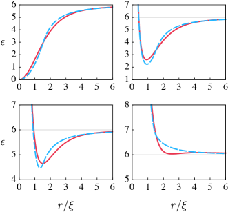
Figure 1: (color online) Comparison of effective one-dimensional radial potentials for the exact solution (solid red) and the variational approximation of Eq. (17) (dashed blue), for $\displaystyle\ell=0$ (upper-left), $\displaystyle\ell=1$ (upper-right), $\displaystyle\ell=2$ (lower-left) and $\displaystyle\ell=3$ (lower-right), for a value $\displaystyle\gamma^{2}=6$ (horizontal grey line) of the potential depth. We see that for $\displaystyle\ell=3$ the effective potentials are entirely above this line, illustrating the relation between the potential depth and angular momentum, and suggesting a loss of bound states for $\displaystyle\gamma^{2}$ decreasing below some threshold.

II.3 Impurity wave functions

We now substitute $\displaystyle\left|\Phi_{0}\right|$ for $\displaystyle\phi_{\alpha}$ in Eq. (10), in order to obtain approximate solutions for the impurity wave functions, and look for bound states, which amounts to requiring $\displaystyle 0<\epsilon<\gamma^{2}$. In polar coordinates, this is done by separating

$$\Psi(r,\varphi)=R(r)e^{\pm\text{i}\ell\varphi},$$ (18)

with $\displaystyle\ell=0,1,2,\text{$\displaystyle\dots$}$ denoting the angular momentum. As for the radial part, it is solved in the two regions $\displaystyle\mathcal{R}_{1}=[0,r_{\alpha}]$ and $\displaystyle\mathcal{R}_{2}=(r_{\alpha},\infty)$. In the first region, we have

$$-\frac{\text{d}^{2}R_{1}}{\text{d}r^{2}}-\frac{1}{r}\frac{\text{d}R_{1}}{\text{d}r}+\left(\frac{\ell^{2}}{r^{2}}+\frac{\alpha^{2}\gamma^{2}}{4}r^{2}\right)R_{1}=\epsilon R_{1}.$$ (19)

Due to the term $\displaystyle\ell^{2}/r^{2}$, these solutions must scale as $\displaystyle R_{1}(r)\propto r^{\ell}$ as $\displaystyle r\rightarrow 0$ for each value of $\displaystyle\ell$, and so the correct solution is given by

$$\displaystyle R_{1}(r) \displaystyle=\mathcal{A}\,r^{\ell}e^{-\frac{\alpha\gamma}{4}r^{2}}\times$$

$$\displaystyle\times M\left(-\frac{\epsilon}{2\alpha\gamma}+\frac{\ell+1}{2},\ell+1;\frac{\alpha\gamma}{2}r^{2}\right),$$ (20)

where $\displaystyle M(a,b;z)$ is the confluent hypergeometric function (CHF) with parameters $\displaystyle a$ and $\displaystyle b$, also known as the first Kummer function Olver et al. (2010), and $\displaystyle\mathcal{A}$ is a normalization constant. Some relevant properties of this function are discussed in Appendix A. In turn, for the second region, we get

$$\frac{\text{d}^{2}R_{2}}{\text{d}r^{2}}+\frac{1}{r}\frac{\text{d}R_{2}}{\text{d}r}+\frac{\gamma_{\alpha}^{2}-\ell^{2}}{r^{2}}R_{2}=\left(\gamma^{2}-\epsilon\right)R_{2}\,,$$ (21)

where $\displaystyle\gamma_{\alpha}=\gamma/\alpha$. Here, the regular solution as required by the vanishing of the wave function as $\displaystyle r\rightarrow+\infty$ is given by

$$R_{2}(r)=\mathcal{A}\,K_{\text{i}\lambda_{\ell}}(qr)\,,$$ (22)

where $\displaystyle\lambda_{\ell}=\sqrt{\gamma_{\alpha}^{2}-\ell^{2}}$ and $\displaystyle q=\sqrt{\gamma^{2}-\epsilon}$ is a real number (for bound states), and $\displaystyle K_{\text{i}\lambda_{\ell}}$ is the modified Bessel function of the second kind of imaginary order $\displaystyle\lambda_{\ell}$ Olver et al. (2010); Dunster (1990). Note that the character of the order (i.e. real or imaginary) does not affect the regularity of the solution (22) by itself Olver et al. (2010), but it rather has a critical role in the bound-state spectrum of the impurity.

III Bound-state spectrum

The impurity spectrum in the vortex is obtained by requiring the continuity of the logarithmic derivative at $\displaystyle r=r_{\alpha}$ Konishi and Paffuti (2009),

$$\left(\ln R_{1}\right)^{\prime}(r_{\alpha})=\left(\ln R_{2}\right)^{\prime}(r_{\alpha})\,,$$ (23)

and solving for $\displaystyle q$. Fig. 2 shows plots of these two functions. We find that Eq. (23) has no solutions for $\displaystyle\gamma_{\alpha}\leq\ell$, as shown in Appendix C.1, so we focus exclusively on the case $\displaystyle\gamma_{\alpha}>\ell$. Consequently, the condition $\displaystyle\lambda_{\ell}=0$ yields critical values $\displaystyle\gamma_{\text{c},\ell}=\alpha\ell$ for the onset of bound states of each angular momenta. Physically, we may interpret this behavior as the impurity seeing the vortex potential with an effective depth proportional to $\displaystyle\lambda_{\ell}^{2}$; indeed, it is straightforward to check that, for each $\displaystyle\ell$, the effective radial potential has the maximum depth $\displaystyle\alpha\gamma(\gamma_{\alpha}-\ell)$. This suggests we can take $\displaystyle\lambda_{\ell}$ (or, further, the related quantity $\displaystyle\Delta_{\ell}\equiv\gamma_{\alpha}-\ell$), as the relevant scale of the problem. This point is illustrated in Fig. 1.

Since we are interested in a vortex with few bound states, as it is the case of a qubit, we focus on a parameter region

$$0<\gamma_{\alpha}<3\,.$$ (24)

Further, in order to obtain qualitative results from Eq. (23), we posit that in the present parameter range the states can be distinguished as shallow states and deep states: the former (latter) sit at the edge (bottom) of the potential, thus being characterized by the long-range, centripetal-like (short-range, harmonic oscillator-like) profile of the vortex density, as implied by Eq. (16) (Eq. (15)) and approximated, respectively, by each branch of Eq. (17).

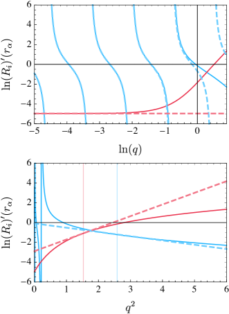
Figure 2: (color online) An instance of Eq. (23) for $\displaystyle\ell=1$ and $\displaystyle\gamma^{2}=6$; the function corresponding to region 1 (2), the deeper (shallower) end of the potential, is in thick red (blue); asymptotics and approximations are the dashed lines of respective color. (Upper panel) the choice of axis shows that there are infinitely many solutions (given by intersections) as $\displaystyle q$ goes to zero, corresponding to shallow states, and the contribution from $\displaystyle\mathcal{R}_{1}$ can be considered constant, while the contribution from $\displaystyle\mathcal{R}_{2}$ is the RHS of (25); (lower panel) solutions for deep states can be obtained by linearization and asymptotics of the logarithmic derivatives, with the vertical lines indicating the linearization points.

III.1 Shallow states

In this case, we can expect $\displaystyle q=\sqrt{\gamma^{2}-\epsilon}\ll 1$, prompting us to look for solutions of Eq. (23) to leading order in $\displaystyle q$. We thus use Eq. (57) to obtain

$$\left(\ln R_{2}\right)^{\prime}(r_{\alpha})=\frac{\lambda_{\ell}}{r_{\alpha}}\cot\left(\lambda_{\ell}\ln\frac{qr_{\alpha}}{2}-\varphi_{\ell}\right)+\mathcal{O}(q^{2}),$$ (25)

where $\displaystyle\varphi_{\ell}\equiv\varphi(\lambda_{\ell})$ is related to the gamma function by $\displaystyle\varphi(\lambda_{\ell})=\arg\Gamma(1+\text{i}\lambda_{\ell})$ Olver et al. (2010); Dunster (1990) (see B.1 for further details). For the LHS of Eq. (23), we have

$$\left(\ln R_{1}\right)^{\prime}(r_{\alpha})=-\frac{\lambda_{\ell}}{r_{\alpha}}\cot\theta_{\ell}+\mathcal{O}(q^{2})\,,$$ (26)

with

$$\theta_{\ell}=\tan^{-1}\left\{\lambda_{\ell}\left[\Delta_{\ell}-2\gamma_{\alpha}\frac{M^{\prime}\left(-\frac{\Delta_{\ell}}{2}+\frac{1}{2},\ell+1;\gamma_{\alpha}\right)}{M\left(-\frac{\Delta_{\ell}}{2}+\frac{1}{2},\ell+1;\gamma_{\alpha}\right)}\right]^{-1}\right\}\,,$$ (27)

where the prime represents differentiation with respect to the argument. The solution of Eq. (23), to leading order in $\displaystyle q$, finally yields the bound-state spectrum for shallow states

$$\frac{E_{p,\ell}}{n_{0}g_{12}}=1-\Lambda_{\ell}^{2}\exp\left(-\frac{2\pi p}{\lambda_{\ell}}\right)\,,$$ (28)

with $\displaystyle p$ the radial quantum number, taking on non-negative integer values, and

$$\Lambda_{\ell}=\frac{\sqrt{2}}{\gamma_{\alpha}}\exp\left(-\frac{(1-\delta_{\ell,0})\pi+\theta_{\ell}-\varphi_{\ell}}{\lambda_{\ell}}\right)\,,$$ (29)

where $\displaystyle\delta_{\ell,0}$ is a Kronecker delta. The description of $\displaystyle p$ must take into account the number of deep states: the integers $\displaystyle p$ indicate the the non-positive branches of the cotangent in (25) at which (23) has solutions, as illustrated in Fig. 2; as $\displaystyle\gamma$ increases, Eq. (25) no longer holds for some values of $\displaystyle p$, as solutions transition from shallow to deep states; hence, the counting of $\displaystyle p$ in (28) start from the number of deep states of angular momentum $\displaystyle\ell$, denoted here by $\displaystyle N_{\text{d}}^{(\ell)}$ and discussed below.

III.2 Deep states

Deep, or confined, states are considered according to the condition

$$\Delta_{\ell}>1,$$ (30)

since, in this regime, it becomes possible for the first parameter of the CHF in Eq. (20) to take on non-positive values,

$$-\frac{\epsilon}{2\alpha\gamma}+\frac{\ell+1}{2}\leq 0\,,$$ (31)

from which (30) is obtained when $\displaystyle\epsilon=\gamma^{2}$, the highest possible value for bound states. If Eq. (31) is satisfied, the solutions to Eq. (20) become integrable on the whole plane, becoming the eigenfunctions of the isotropic quantum harmonic oscillator (check Appendix A.1 for a more complete discussion around this issue). This observation leads us to define the quantity

$$\delta\epsilon_{1}\equiv-\frac{\epsilon}{2\alpha\gamma}+\frac{\ell+1}{2}+p\,,$$ (32)

for $\displaystyle p=0,1,2,\text{$\displaystyle\dots$}$, and to look for solutions of Eq. (23) to first order in $\displaystyle\delta\epsilon_{1}$ as the leading order contributions to its LHS. We thus require the first derivative of the CHF with respect to its first parameter evaluated at non-positive integers; one approach to this problem is presented in Appendix A.2.

Furthermore, the criterion in Eq. (30) can be easily generalized to a more precise condition regarding the number of deep states, and we find that

$$-1<\Delta_{\ell}-2N_{\text{d}}^{(\ell)}<1\,,$$ (33)

for $\displaystyle N_{\text{d}}^{(\ell)}=0,1,2,\dots$, if there are $\displaystyle N_{\text{d}}^{(\ell)}$ deep states of angular momentum $\displaystyle\pm\ell$, accounting for the sign-degeneracy in Eq. (18). Hence, within the parameter range given in (24), we have at most $\displaystyle N_{\text{d}}^{(0)}=N_{\text{d}}^{(1)}=1$ and $\displaystyle N_{\text{d}}^{(2)}=0$, corresponding to the state $\displaystyle p=0$, for $\displaystyle\ell=0$ and for $\displaystyle\ell=1$, and none for $\displaystyle\ell=2$. According to Eqs. (46) and (51), for $\displaystyle p=0$ the LHS of Eq. (23) becomes

$$\displaystyle\left(\ln R_{1}\right)^{\prime}(r_{\alpha})=$$

$$\displaystyle=-\frac{\Delta_{\ell}}{r_{\alpha}}+\frac{1}{r_{\alpha}}\frac{(\ell,\gamma_{\alpha})!}{\gamma_{\alpha}^{\ell}e^{-\gamma_{\alpha}}}\left(\ell+1-\frac{\epsilon}{\alpha\gamma}\right)+\mathcal{O}(\delta\epsilon_{1}^{2})\,,$$ (34)

where $\displaystyle(\ell,\gamma_{\alpha})!$ is given in Eq. (52). The RHS of Eq. (23), on the other hand, has a weak dependence on $\displaystyle\epsilon$ for sufficiently large $\displaystyle\gamma$, since at that point the solution (22) transitions from an oscillatory to an exponentially decaying behavior, as discussed in B.2. We can write $\displaystyle q=\lambda_{\ell}/r_{\alpha}+\delta\epsilon_{2}+\mathcal{O}(\delta\epsilon_{2}^{2})$, and expand the RHS of Eq. (23) to first order in

$$\delta\epsilon_{2}\equiv-\frac{\epsilon-\left(\gamma^{2}-\lambda_{\ell}^{2}/r_{\alpha}^{2}\right)}{2\lambda_{\ell}/r_{\alpha}}=\frac{1}{r_{\alpha}}\left(\frac{\gamma_{\alpha}^{2}+\ell^{2}}{2\lambda_{\ell}}-\frac{\epsilon}{\alpha^{2}\lambda_{\ell}}\right)\,.$$ (35)

We then find

$$\displaystyle\left(\ln R_{2}\right)^{\prime}(r_{\alpha})=$$

$$\displaystyle=-\frac{\lambda_{\ell}\mathcal{K}_{\ell}}{r_{\alpha}}-\frac{\lambda_{\ell}\mathcal{K}_{\ell}^{2}}{r_{\alpha}}\left(\frac{\gamma_{\alpha}^{2}+\ell^{2}}{2\lambda_{\ell}}-\frac{\epsilon}{\alpha^{2}\lambda_{\ell}}\right)+\mathcal{O}(\delta\epsilon_{2}^{2})\,,$$ (36)

where

$$\mathcal{K}_{\ell}\sim\frac{\beta}{\lambda_{\ell}^{1/3}}\left(1+\frac{1}{4\lambda_{\ell}}\right)+\mathcal{O}(\lambda_{\ell}^{-2})\,,$$

with $\displaystyle\beta=6^{\frac{1}{3}}\Gamma\left(\frac{2}{3}\right)/\Gamma\left(\frac{1}{3}\right)\approx 0.918$, is an asymptotic approximation of $\displaystyle\mathcal{K}_{\ell}\equiv-\left(\ln K_{\text{i}\lambda_{\ell}}\right)^{\prime}(\lambda_{\ell})$ for large $\displaystyle\lambda_{\ell}$; these results are derived in B.2. Equating (34) to (36) and solving in order to $\displaystyle\delta\epsilon_{1}$, yields

$$\displaystyle\frac{E_{p=0,\ell}}{\hbar\omega} \displaystyle=\left(\ell+1\right)\left(1-\Omega_{\ell}\right)$$

$$\displaystyle+\left(\frac{\gamma_{\alpha}^{2}+\ell^{2}}{2\gamma_{\alpha}}-\frac{\Delta_{\ell}-\lambda_{\ell}\mathcal{K}_{\ell}}{\gamma_{\alpha}\mathcal{K}_{\ell}^{2}}\right)\Omega_{\ell}$$ (37)

with

$$\Omega_{\ell}=\left(1+\frac{1}{\beta^{2}}\frac{\lambda_{\ell}^{5/3}}{\lambda_{\ell}+1/2}\frac{(\ell,\gamma_{\alpha})!}{\gamma_{\alpha}^{\ell+1}e^{-\gamma_{\alpha}}}\right)^{-1}\,,$$ (38)

and

$$\omega=\frac{\alpha}{2}\frac{\hbar}{m_{2}\hat{\xi}^{2}}\,,\quad\hat{\xi}^{2}=\frac{\hbar^{2}}{2n_{0}\sqrt{g_{11}m_{1}g_{12}m_{2}}}\,.$$ (39)

In particular, for $\displaystyle\ell=0$, Eq. (37) gives the energy of the ground state, with (38) reducing to

$$\Omega_{0}=\left(1+\frac{\gamma_{\alpha}^{2/3}}{\beta^{2}}\frac{e^{\gamma_{\alpha}}-1}{\gamma_{\alpha}+1/2}\right)^{-1}\,,$$ (40)

for $\displaystyle\gamma_{\alpha}>1$, i.e. whenever it is a deep state.

We can then write down the elements of the bound-state spectrum in the following way:

$$E_{p,\ell}=\begin{cases}n_{0}g_{12}\mathcal{E}_{p,\ell}^{(\text{s})}&,\,p-N_{\text{d}}^{(\ell)}\geq 0\\ \hbar\omega\mathcal{E}_{p,\ell}^{(\text{d})}&,\,p-N_{\text{d}}^{(\ell)}<0\end{cases}\,,$$

where $\displaystyle\mathcal{E}_{p,\ell}^{(\text{s})}$ is given by the RHS of Eq. (28) and $\displaystyle\mathcal{E}_{p=0,\ell}^{(\text{d})}$ by the RHS of Eq. (37), and with $\displaystyle N_{\text{d}}^{(\ell)}$ is determined for each $\displaystyle\gamma^{2}$ according to (33) and the accuracy of the deep state approximation.

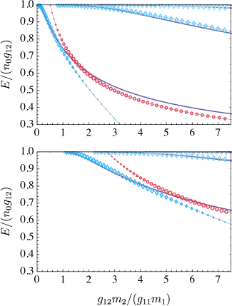
Figure 3: (color online) Comparison of approximate to numerical results for $\displaystyle\ell=0$ (upper panel) and $\displaystyle\ell=1$ (lower panel). Each group of curves corresponds to a value of the radial quantum number $\displaystyle p$, starting from $\displaystyle p=0$; thick solid purple lines give the numerical solution; thin solid gray lines marked with blue diamonds (red circles) give the solutions from the shallow-state (deep-state) approximation, with the size of the markers being a function of the difference of approximate and numerical solutions for equal $\displaystyle p$ at each $\displaystyle\gamma^{2}$. The finite-size cut-off corresponds to a trap of radius $\displaystyle R=1000$ healing lengths, according to Eq. (41), while the horizontal axis ranges within the interval (24).

III.3 Features of the energy spectrum

The energies of shallow and deep bound state are explicitly associated to two different energy scales $\displaystyle n_{0}g_{12}$ and $\displaystyle\hbar\omega$; while the former is directly sourced from the microscopic dynamics of the system, being proportional to the interspecies coupling $\displaystyle g_{12}$, the latter can be written in terms of an emergent length scale that is not the characteristic healing length of the condensate, but rather a geometric mean

$$\hat{\xi}=\sqrt{\xi\zeta}\,,\quad\zeta^{2}=\frac{\hbar^{2}}{2n_{0}m_{2}g_{12}}\,,$$

where $\displaystyle\zeta$ can be interpreted as an impurity-to-BEC penetration length. This interpretation becomes clearer by writing the square root of the dimensionless potential-well depth $\displaystyle\gamma^{2}$ as

$$\gamma=\sqrt{\frac{g_{12}m_{2}}{g_{11}m_{1}}}=\frac{\xi}{\zeta}\,,$$

and we see that an increase in depth of the potential can be interpreted, instead, as increased confinement according to the two emergent length scales. This also implies that, at least formally, $\displaystyle\gamma^{2}$ may increase arbitrarily while $\displaystyle\hat{\xi}$, as well as $\displaystyle\omega$, remain finite. As depicted in Fig. 3, this disparity of scales indicates that, for each $\displaystyle\ell$, there can be a sizeable gap between deep states and shallow states relative to the gap between shallow states of different $\displaystyle p$.

Figure 3 shows excellent agreement between the approximate and numerical solutions, though there is a noticeable divergence with increasing $\displaystyle\gamma$. This is rooted in the variational approximation (17): notice that Eq. (37) tends to the spectrum of the harmonic oscillator with increasing $\displaystyle\gamma$, accordingly with the short-range behavior of the exact vortex profile (15). However, the slope at $\displaystyle r=0$ of the approximate solution (17) is smaller than that of the exact one, as fixed by the variational procedure. This discrepancy thus becomes starker with increased depth, with the spectrum of deep states being directly proportional to this slope as shown in Eq. (39).

An interesting feature of the impurity spectrum has to do with the energy levels near the edge of the potential. In this region, the spectrum is rich in crossovers and accidental degeneracies, resulting from the visibly faster decrease in energy of states of higher angular momenta. This can be understood in light of the competition between the centrifugal barrier and the vortex potential: at the onset of the first bound states, the long-range profile of the potential is canceled by the centrifugal term, rendering the effective potential more confining than that of states of lower angular momenta. This behavior is displayed in Fig. (4).

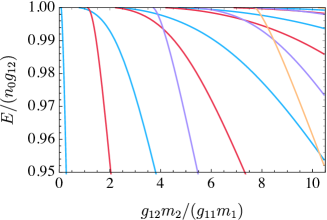
Figure 4: (color online) Numerical values of the spectrum as a function of $\displaystyle\gamma^{2}$ fpr $\displaystyle\ell=0$ (blue), $\displaystyle\ell=1$ (red), $\displaystyle\ell=2$ (purple) and $\displaystyle\ell=3$ (orange). Energy levels have a finite-size cut-off corresponding to a trap of radius $\displaystyle R=1000$ healing lengths.

IV Finite size and physical bound states

The spectrum obtained in Eq. (28) for the shallow states indicates that there are, in fact, infinitely many bound-state solutions for each $\displaystyle\ell<\gamma_{\alpha}$, which can be attributed to the slow algebraic growth of the vortex profile. Most of these are not physical solutions, however. To see this, we must consider that there is a natural cut-off imposed by the finite size of the trap, which is not merely a practical limitation: this is required by the stability of the vortex configuration, whose energy diverges logarithmically with the system size Lundh et al. (1998), and also due to the impossibility of long-range order in low dimensions, as imposed by the Mermin-Wagner theorem. We can account for this simply by requiring that the classical turning point (in the radial coordinate) of the putative bound state is lying within the domain of the BEC. Hence, assuming a disk-like trap of radius $\displaystyle R\gg\xi$ , we have the quantitative condition

$$1-\frac{E_{p,\ell}}{n_{0}g_{12}}>\frac{\xi^{2}}{\alpha^{2}R^{2}}\,,$$ (41)

which, together with Eq. (28), imposes a condition in $\displaystyle\gamma^{2}$ for a bound state $\displaystyle(p,\ell)$ to be contained in the BEC. Fig. (3) shows comparisons between numerical and approximate solutions, where the cut-off (41) for a trap of size $\displaystyle R=1000\xi$ was included. It is clear that for each value of $\displaystyle\gamma$ there are only a finite number of bound states of the vortex, while those violating the condition Eq. (41) can be seen as bound states of the trapping potential.

Solutions to Eq. (41) can be found semi-analytically, as discussed in C.2, yielding the critical condition

$$\left.\frac{g_{12}m_{2}}{g_{11}m_{1}}\right|_{p,\ell}>\alpha^{2}\ell^{2}+\frac{c_{p,\ell}^{-2}}{\ln\left(\frac{R}{r_{p,\ell}\xi}\right)^{2}}$$ (42)

for the onset of the bound state $\displaystyle(p,\ell)$. The coefficients $\displaystyle c_{p,\ell}$ and $\displaystyle r_{p,\ell}$ for the first few bound states are given in Table (1). Figure LABEL:fig:Diagram-regimes gives a diagram of regimes of the vortex potential well, providing the number of bound states for each point in the $\displaystyle(R/\xi,\gamma^{2})$ parameter space.

Moreover, we can expect that imposing this cut-off a posteriori has negligible effects on the physical solutions of Eq. (10) since, in practice, the condition $\displaystyle R\gg\xi$ is implied by the thermodynamic limit. The caveat is that the possible highly-excited, highly-delocalized states may become affected by the trapping potential, but this correction can, in principle, be accounted for using perturbation theory. For this reason, the RHS of Eq. (42) is a tight lower bound of the critical value for the onset of the bound state $\displaystyle(p,\ell)$ .

V Experimetnal considerations

Recent experimental work with Yb-${}^{7}\text{Li}$ mixtures Schäfer et al. (2018) provides a realistic platform for the realization of this system: by virtue of the substantial mass imbalance of $\displaystyle m_{\text{Yb}}/m_{\text{Li}}\approx 25$, the impurity-to-vortex decoupling condition in Eq. (9) is within reach by immersion of Yb impurities (either fermionic ${}^{173}\text{Yb}$, or bosonic ${}^{174}\text{Yb}$ Schäfer et al. (2018)) in a ${}^{7}\text{Li}$ condensate, while also increasing $\displaystyle\gamma^{2}$.

Nevertheless, the tunability of the latter is still necessary, since a vortex supporting only a few bound states requires $\displaystyle\gamma^{2}$ one order of magnitude below that; thus, Feshbach resonances would be a crucial element in this realization. Coincidentally, the realizations of Ref. Schäfer et al. (2018) exploits a fairly accessible Feshbach resonance of ${}^{7}\text{Li}$ in order to produce a stable and sizeable BEC of this species Gross and Khaykovich (2008). The modest interspecies scattering found for Yb-${}^{7}\text{Li}$ ($\displaystyle\sim 1\,\text{nm}$) Schäfer et al. (2018) then means that the parameter range in Eq. (24) is well within reach by tuning the ${}^{7}\text{Li}$ intra-species scattering to tens of nanometers.

In a quasi-2D BEC, such as considered presently, couplings become renormalized by the transversal length scale $\displaystyle a_{\perp}$ of the harmonic trap Salasnich et al. (2002); Krüger et al. (2007); Young-S. et al. (2010), as $\displaystyle g_{ij}\propto a_{ij}/a_{\perp}$ if $\displaystyle a_{ij}$ is the scattering length between species $\displaystyle i$ and $\displaystyle j$. While this multiplicative factor has no effect on $\displaystyle\gamma^{2}\propto g_{12}/g_{11}$, the decoupling parameter $\displaystyle\kappa^{2}/\gamma^{2}$ (see Eq. (9)) is proportional to $\displaystyle g_{11}$ alone. Typical trapping frequencies of tens of kHz yield a transversal length of hundreds of nanometers for ⁷Li, which further reduces the decoupling parameter Zhang et al. (2008). Additional flexibility comes from the usage of box potentials Gaunt et al. (2013); Gotlibovych et al. (2014), which are able to produce homogeneous condensates in a more controllable way Chomaz et al. (2015); Desbuquois et al. (2014).

Another important aspect pertains to the relation of the energy scale $\displaystyle n_{0}g_{12}$ of the spectrum to the temperature. We find that for a peak density (in volume) of $\displaystyle\sim 10^{4}\,\text{cm}^{-3}$, the Yb-${}^{7}\text{Li}$ mixture yields $\displaystyle n_{0}g_{12}/k_{\text{B}}\propto 10^{2}\,\text{nK}$, meaning that the typical energy gap is much larger than the temperature of the system. This suggests that we might be in good position to further exploit these impurity bound states as physical qubits Shaukat et al. (2017), thus paving the stage for a possible quantum information platform operating in the kHz range.

VI Conclusion

Starting from a variational ansatz for the vortex profile in a quasi two-dimensional Bose-Einstein condensate, which has been shown to be in excellent agreement with the numerical calculations, we have obtained the eigenstates and the eigenvalues of the vortex-impurity problem. Our method consists in imposing regularity conditions (continuity and finite derivative) at the crossing of the vortex piecewise solution, the point marking the transition between the core ($\displaystyle\sim r$, as $\displaystyle r\rightarrow 0$) and the edge ($\displaystyle\sim 1/r^{2}$, as $\displaystyle r\rightarrow\infty$) of the vortex. As a result, we are able to obtain analytic expression for both shallow and deep bound states, respectively lying at the edge and at the bottom of the effective potential experienced by the impurity when interacting with the vortex. A comparison with numerical results reveals that, for the states of angular momentum $\displaystyle\ell=0,1$, our analytical results appear to be accurate in their respective range of validity. For the general case, for states lying at the vortex profile transition, analytical expressions are, in general, not available explicitly. We point out that similar results have been obtained in the study of the one-dimensional $\displaystyle 1/x^{2}$ potential Essin and Griffiths (2006), and that a similar approach was used in the study of core-to-coreless vortex transition in multicomponent superfluids Catelani and Yuzbashyan (2010).

The consideration of heavy impurities immersed in a gas of light particles, as made possible by the recent experiments allowing for the controllable mixture of Li and Yb Hansen et al. (2013); Khramov et al. (2014); Schäfer et al. (2018), allows the investigation of the polaron physics in a fashion opposed to the usual solid-state scenarios, where the impurity (electron) is much lighter that the host particles (ions) Fröhlich et al. (1950). Moreover, our calculations may also contribute for future studies of the so-called “Tkachenko polaron”, a quasi-particle resulting from the coupling between an impurity and a vortex lattice vibration in rotating Bose-Einstein condensates Caracanhas et al. (2013). Here, the vortex-induced trapping may significantly change the features of the polaron.

More crucially, our findings show that it is possible to tune the value of the impurity-BEC interaction to isolate two deep (localized) bound states deep in the core of the vortex, making it possible to promote the impurity into a qubit, an essential element for applications in quantum information theory. In the future, it will be crucial to investigate the relevant beyond mean-field effects, namely the coupling with the quantum excitations of the BEC (phonons), a task that we believe essential for the complete characterization of the qubit performance. Due to the scalability of the number of vortices in a two-dimensional BEC, we expect this to become an interesting alternative to the one-dimensional qubits made of dark-solitons Shaukat et al. (2019), therefore offering a possible alternative for a quantum information platform operating with acoustic degrees of freedom in a near future.

Appendix A Properties of the confluent hypergeometric function

A.1 Zeros and monotonicity

The confluent hypergeometric function (CHF) can be expressed as a generalized hypergeometric series,

$$M(a,b;x)=\sum_{m=0}^{\infty}\frac{(a)_{m}}{(b)_{m}}\frac{x^{m}}{m!}\,,$$ (43)

where

$$(a)_{m}=\frac{\Gamma(a+m)}{\Gamma(a)}=a(a+1)\text{$\displaystyle\dots$}(a+m-1)\,,$$ (44)

for any $\displaystyle a\in\mathbb{C}$, is the Pochhammer symbol, also known as the rising factorial; the CHF is an entire function of its argument, implying that the series (43) has an infinite radius of convergence. Olver et al. (2010)

From this definition, it is clear that for $\displaystyle x\in[0,+\infty[$ the CHF has no zeros for any real $\displaystyle a,b\geq 0$ and that it is positive and increasing. Olver et al. (2010) Moreover, when $\displaystyle a<0$ it has $\displaystyle\lceil-a\rceil$ positive zeros, and when $\displaystyle a=-n$, with $\displaystyle n=0,1,2,\text{$\displaystyle\dots$}$, and $\displaystyle b=\beta+1$, with $\displaystyle\beta$ real and non-negative, the CHF reduces to the $\displaystyle n$th generalized Laguerre polynomial,

$$M(-n,\beta+1;x)=\frac{n!}{(\beta+1)_{n}}L_{n}^{(\beta)}(x)\,;$$ (45)

the series in (43) reduces to an $\displaystyle n$th-degree polynomial since $\displaystyle(-n)_{m}$ vanishes for $\displaystyle m\geq n-1$, as per (44). Olver et al. (2010) In particular, the generalized Laguerre polynomials comprise the solutions of the isotropic quantum harmonic oscillator. Olver et al. (2010)

A.2 Derivative with respect to the first parameter

Suppose that in Eq. (43) we have $\displaystyle a=-n+\delta a$ with $\displaystyle n=0,1,2,\text{$\displaystyle\dots$}$, with $\displaystyle\delta a$ real and of small absolute value, and $\displaystyle b=\beta+1$, with $\displaystyle\beta$ real and non-negative. Taylor-expanding with regard to the first parameter we have

$$\displaystyle M(-n+\delta a,\beta+1;x)=$$

$$\displaystyle=\frac{n!}{(\beta+1)_{n}}L_{n}^{(\beta)}(x)+\delta a\,\tilde{M}_{n}^{(\beta)}(x)+O(\delta a^{2})\,,$$ (46)

where we use (45) for the zeroth-order term, and define

$$\tilde{M}_{n}^{(\beta)}(x)=\left.\frac{\partial}{\partial a}M\left(a,\beta+1;x\right)\right|_{a=-n},$$ (47)

for $\displaystyle n=0,1,2,\text{$\displaystyle\dots$}$. For $\displaystyle n=0$, we can use Eq. (38a) of Ref. Ancarani and Gasaneo (2008) and rewrite it as

$$\tilde{M}_{0}^{(\beta)}(x)=\frac{1}{\beta+1}\sum_{m=0}^{\infty}\frac{x^{m+1}}{(m+1)(\beta+2)_{m}}\,;$$ (48)

notice that

$$\frac{\text{d}}{\text{d}x}\tilde{M}_{0}^{(\beta)}(x)=\frac{1}{\beta+1}M(1,\beta+2;x)\,,$$

since $\displaystyle(1)_{m}=m!$ according to (44); this CHF can be written as Olver et al. (2010) (p. 328, Eq. (13.6.5))

$$M(1,\beta+2;x)=(\beta+1)x^{-\beta-1}e^{x}(\beta,x)!\,,$$ (49)

where $\displaystyle(\beta,x)!$ is a rewriting of the incomplete gamma function foo (a),

$$(\beta,x)!=\gamma(\beta+1,x)=\int_{0}^{x}\text{d}t\,t^{\beta}e^{-t}\,,$$ (50)

so that we can write (48) as an integral of (49):

$$\tilde{M}_{0}^{(\beta)}(x)=\int_{0}^{x}\frac{\text{d}y}{y}\frac{(\beta,y)!}{y^{\beta}e^{-y}}\,.$$ (51)

Further, for $\displaystyle\beta=\ell$ a non-negative integer, it follows from (50) that Olver et al. (2010) (p. 177, Eq. (8.4.7))

$$\frac{(\ell,x)!}{\ell!}=1-e^{-x}\sum_{k=0}^{\ell}\frac{x^{k}}{k!}\,.$$ (52)

In turn, for $\displaystyle n\geq 1$ we have Olver et al. (2010) (p. 325, Eq. (13.3.1))

$$M(a,b;x)=\frac{(a-b)M(a-1,b;x)}{2a-b+x}+\frac{aM(a+1,b;x)}{2a-b+x}\,;$$ (53)

identifying parameters, expanding both sides to first order in $\displaystyle\delta a$ and matching powers, we find

$$\displaystyle n=1:\quad \displaystyle\left(\beta+1\right)\tilde{M}_{1}^{(\beta)}(x)=-\frac{x}{\beta+1}+\frac{\left(\beta,x\right)!}{x^{\beta}e^{-x}}+\left(1+\beta-x\right)\int_{0}^{x}\frac{\text{d}y}{y}\frac{(\beta,y)!}{y^{\beta}e^{-y}}\,,$$ (54)

$$\displaystyle n\geq 2:\quad \displaystyle\left(\beta+n\right)\tilde{M}_{n}^{(\beta)}(x)-(2n+\beta-x-1)\tilde{M}_{n-1}^{(\beta)}(x)+(n-1)\tilde{M}_{n-2}^{(\beta)}(x)=\sum_{k=0}^{2}\binom{2}{k}\frac{(-1)^{k}(n-k)!}{(\beta+1)_{n-k}}L_{n-k}^{(\beta)}(x)\,;$$ (55)

for $\displaystyle n\geq 2$ we use (45) to write the RHS in terms of generalized Laguerre polynomials, while for $\displaystyle n=1$ we use (45), and (49) along with the recurrence relation of the incomplete gamma function Olver et al. (2010) (p. 178, Eq. (8.8.1))

$$\beta\left(\beta-1,x\right)!=x^{\beta}e^{-x}+\left(\beta,x\right)!\,.$$ (56)

Appendix B Asymptotics of the Bessel-$\displaystyle K$ of imaginary order and its derivatives

B.1 Bessel-$\displaystyle K$ of imaginary order for small argument

For $\displaystyle x\in\mathbb{R}^{+}$ small and $\displaystyle\lambda\in\mathbb{R}^{+}$, we have the limiting behavior Olver et al. (2010); Dunster (1990)

$$K_{\text{i}\lambda}(x)=-\sqrt{\frac{\pi}{\lambda\sinh(\pi\lambda)}}\sin\left(\lambda\ln\frac{x}{2}-\varphi(\lambda)\right)+\mathcal{O}(x^{2})\,,$$ (57)

where the function $\displaystyle\varphi(\lambda)$ is given by

$$\varphi(\lambda)=\arg\Gamma(1+\text{i}\lambda)\,,$$ (58)

with the branch defined so that $\displaystyle\varphi$ is continuous for $\displaystyle 0<\lambda<\infty$ and $\displaystyle\lim_{\lambda\rightarrow 0}\varphi(\lambda)=0$ Dunster (1990). For large $\displaystyle\lambda$, this can be approximated using Stirling’s formula Olver et al. (2010), yielding

$$\varphi(\lambda)\sim\frac{\pi}{4}+\lambda\left(\ln\lambda-1\right)+\mathcal{O}(\lambda^{-2})\,,$$ (59)

while for small $\displaystyle\lambda$, the gamma function can be approximated by the series Olver et al. (2010) (p. 139, Eq. (5.7.3))

$$\displaystyle\log\Gamma(1+z) \displaystyle=-\log(1+z)+(1-\gamma_{\text{E}})z$$

$$\displaystyle+\sum_{k=2}^{\infty}(-1)^{k}\left(\zeta(k)-1\right)\frac{z^{k}}{k}\,,$$ (60)

for $\displaystyle\left|z\right|<2$, where $\displaystyle\gamma_{\text{E}}\approx 0.5572$ is the Euler-Mascheroni constant and $\displaystyle\zeta$ the Riemann-zeta function, giving

$$\displaystyle\varphi(\lambda) \displaystyle=-\gamma_{\text{E}}\lambda-\sum_{k=1}^{\infty}(-1)^{k}\frac{\zeta(2k+1)}{2k+1}\lambda^{2k+1}\,.$$ (61)

B.2 Bessel-$\displaystyle K$ of imaginary order at the transition point

In deriving Eq. (36), we perform a Taylor expansion

$$\displaystyle\left.\frac{\text{d}\ln K_{\text{i}\lambda_{\ell}}(qr)}{\text{d}r}\right|_{r=r_{\alpha},q=\frac{\lambda_{\ell}}{r_{\alpha}}+\delta\epsilon_{2}}=$$

$$\displaystyle=-\frac{\lambda_{\ell}}{r_{\alpha}}\mathcal{K}_{1}(\lambda_{\ell})-\delta\epsilon_{2}\left(\mathcal{K}_{1}(\lambda_{\ell})+\lambda_{\ell}\mathcal{K}_{2}(\lambda_{\ell})\right)+\mathcal{O}(\delta\epsilon_{2}^{2})$$ (62)

where we define a family of functions specified as

$$\mathcal{K}_{n}(\lambda_{\ell})=-\left(\ln K_{\text{i}\lambda_{\ell}}\right)^{(n)}(\lambda_{\ell})\,,$$ (63)

that is, the $\displaystyle n$th derivative of the function $\displaystyle-\ln K_{\text{i}\lambda_{\ell}}(x)$ evaluated at the so-called transition point $\displaystyle x=\lambda_{\ell}$. For $\displaystyle n=1,2$, we have explicitly

$$\mathcal{K}_{1}(\lambda_{\ell})=-\frac{K_{\text{i}\lambda_{\ell}}^{\prime}\left(\lambda_{\ell}\right)}{K_{\text{i}\lambda_{\ell}}\left(\lambda_{\ell}\right)}\,,$$ (64)

$$\mathcal{K}_{2}(\lambda_{\ell})=-\frac{K_{\text{i}\lambda_{\ell}}^{\prime\prime}\left(\lambda_{\ell}\right)}{K_{\text{i}\lambda_{\ell}}\left(\lambda_{\ell}\right)}+\left(\frac{K_{\text{i}\lambda_{\ell}}^{\prime}\left(\lambda_{\ell}\right)}{K_{\text{i}\lambda_{\ell}}\left(\lambda_{\ell}\right)}\right)^{2}\,,$$ (65)

where $\displaystyle\lambda_{\ell}>\sqrt{2\ell+1}$, $\displaystyle\ell\in\mathbb{N}_{0}$. Note that $\displaystyle\mathcal{K}_{\ell}\equiv\mathcal{K}_{1}(\lambda_{\ell})$, as defined in the main text.

We have, for any $\displaystyle z,\nu\in\mathbb{C}$ Olver et al. (2010) (p. 252, Eqs. (10.29.2)),

$$K_{\nu}^{\prime}(z)=\frac{\nu}{z}K_{\nu}(z)-K_{\nu+1}(z)\,,$$ (66)

$$K_{\nu}^{\prime\prime}(z)=\left(1+\frac{\nu(\nu-1)}{z^{2}}\right)K_{\nu}(z)+\frac{1}{z}K_{\nu+1}(z)\,;$$ (67)

in particular, for $\displaystyle z=\lambda$ and $\displaystyle\nu=\text{i}\lambda$, $\displaystyle\lambda\in\mathbb{R}$, we have

$$\displaystyle K_{\text{i}\lambda}^{\prime}(\lambda) \displaystyle=\text{i}K_{\text{i}\lambda}(\lambda)-K_{1+\text{i}\lambda}(\lambda)\,,$$ (68)

$$K_{\text{i}\lambda}^{\prime\prime}(\lambda)=-\frac{\text{i}}{\lambda}K_{\text{i}\lambda}(\lambda)+\frac{1}{\lambda}K_{1+\text{i}\lambda}(\lambda)=-\frac{1}{\lambda}K_{\text{i}\lambda}^{\prime}(\lambda)\,,$$ (69)

and then Eq. (65) can then be written in terms of $\displaystyle\mathcal{K}_{\ell}$ only as

$$\mathcal{K}_{2}(\lambda_{\ell})=-\frac{\mathcal{K}_{\ell}}{\lambda_{\ell}}+\mathcal{K}_{\ell}^{2}\,.$$ (70)

Substituting (70) into (62), we obtain Eq. (36).

We have reduced the problem to computing asymptotic expressions of functions $\displaystyle K_{\text{i}\lambda}(\lambda)$ and $\displaystyle K_{\text{i}\lambda}^{\prime}(\lambda)$ of $\displaystyle\lambda$, for $\displaystyle\lambda>1$. We make use of the integral representation Olver et al. (2010) (p. 252, Eq. (10.32.9))

$$K_{\nu}(z)=\int_{0}^{\infty}\text{d}t\,e^{-z\cosh t}\cosh(\nu t)\,,$$ (71)

or $\displaystyle\left|\text{ph}z\right|<\frac{\pi}{2}$ and any $\displaystyle\nu\in\mathbb{C}$. Substituting $\displaystyle\nu=\text{i}\lambda$ and $\displaystyle z=\lambda$, we have

$$\displaystyle K_{\text{i}\lambda}(\lambda) \displaystyle=\int_{0}^{\infty}\text{d}t\,e^{-\lambda\cosh t}\cos(\lambda t)$$

$$\displaystyle=\frac{1}{2}\int_{-\infty}^{+\infty}\text{d}t\,e^{-\lambda\cosh t+\text{i}\lambda t}\,,$$ (72)

and we find

$$K_{\text{i}\lambda}^{\prime}(\lambda)=\frac{\text{d}K_{\text{i}\lambda}(\lambda)}{\text{d}\lambda}-\frac{1}{2}\int_{-\infty}^{+\infty}\text{d}t\,\text{i}te^{-\lambda\cosh t+\text{i}\lambda t}\,.$$ (73)

We can thus obtain asymptotic forms of $\displaystyle K_{\text{i}\lambda}(\lambda)$ and $\displaystyle K_{\text{i}\lambda}^{\prime}(\lambda)$ from two $\displaystyle\lambda$-dependent integrals

$$\mathcal{I}_{k}=\frac{1}{2}\int_{-\infty}^{+\infty}\text{d}t\,\left(\text{i}t\right)^{k}e^{-\lambda\cosh t+\text{i}\lambda t}\,,\quad k=0,1\,.$$ (74)

We note that $\displaystyle\cosh t=2\sinh^{2}\frac{t}{2}+1$ and transform the integration coordinate as

$$\sinh\frac{t}{2}=\frac{x}{2}\Rightarrow\text{dt}=\frac{\text{d}x}{\sqrt{1+\left(\frac{x}{2}\right)^{2}}}\,,$$

yielding

$$\mathcal{I}_{k}=\frac{e^{-\lambda}}{2}\int_{-\infty}^{+\infty}\text{d}x\,\frac{e^{-\lambda g(x)}}{\sqrt{1+\left(\frac{x}{2}\right)^{2}}}\left(\text{i}t(x)\right)^{k}\,,\quad k=0,\,1\,,$$ (75)

with $\displaystyle t(x)=2\text{i}\sinh^{-1}\frac{x}{2}$ and $\displaystyle g(x)=\frac{x^{2}}{2}-2\text{i}\sinh^{-1}\frac{x}{2}$. We now perform a stationary phase approximation Olver (1997): the function $\displaystyle g$ is stationary for $\displaystyle x=x_{*}=\text{i}\sqrt{2}$ and, expanding to subleading order in $\displaystyle\xi=x-x_{*}$, we have

$$g(x_{*}+\xi)=\left(\frac{\pi}{2}-1\right)+\frac{\text{i}\sqrt{2}}{3}\xi^{3}+\frac{\xi^{4}}{2}+\mathcal{O}(\xi^{5})\,.$$ (76)

Here, we include the subleading term to make a point that the integral is convergent; in what follows, however, we include only the leading order in $\displaystyle\xi$ in the exponent, meaning we assume that contributions to the integral (75) result dominantly from the oscillatory factor rather than from the decaying one, the latter granting only (implicitly) the convergence of the integral. We then have

$$\mathcal{I}_{k}\sim\frac{e^{-\frac{\pi\lambda}{2}}}{2}\int_{-\infty}^{+\infty}\text{d}\xi\,\frac{e^{-\frac{\text{i}\sqrt{2}\lambda}{3}\xi^{3}}}{\sqrt{1+\left(\frac{x_{*}+\xi}{2}\right)^{2}}}p_{k}(\xi)\,,$$ (77)

where we have made $\displaystyle p_{k}(\xi)=\left(\text{i}t(x_{*}+\xi)\right)^{k}$ , so that $\displaystyle p_{0}(\xi)=1$ and

$$p_{1}(\xi)=-\frac{\pi}{2}+\sqrt{2}\text{i}\xi-\frac{1}{2}\left(\text{i}\xi\right)^{2}+\frac{\sqrt{2}}{3}\left(\text{i}\xi\right)^{3}-\frac{1}{2}\left(\text{i}\xi\right)^{4}+\mathcal{O}(\xi^{5})\,.$$ (78)

Moreover, we consider that the variation of the denominator of the integrand is negligible in the presence of the exponential factor, so that we have

$$\int_{-\infty}^{+\infty}\frac{\text{d}\xi\,e^{-\frac{\text{i}\sqrt{2}\lambda}{3}\xi^{3}}}{\sqrt{1+\left(\frac{x_{*}+\xi}{2}\right)^{2}}}p_{k}(\xi)\approx\sqrt{2}\int_{-\infty}^{+\infty}\text{d}\xi\,e^{-\frac{\text{i}\sqrt{2}\lambda}{3}\xi^{3}}p_{k}(\xi)\,,$$ (79)

and, then,

$$\displaystyle\frac{1}{2}\int_{-\infty}^{+\infty}\text{d}x\,e^{-\frac{\text{i}\sqrt{2}\lambda}{3}\xi^{3}}p_{k}(\xi) \displaystyle=\text{Re}\left(\int_{0}^{\infty}\text{d}\xi\,e^{-\frac{\text{i}\sqrt{2}\lambda}{3}\xi^{3}}p_{k}(\xi)\right)\,,$$ (80)

since $\displaystyle p_{k}(-\xi)$ is the complex conjugate of $\displaystyle p_{k}(\xi)$. We have the integral identity in Ref. Jeffrey and Zwillinger (2007) (p. 337, Eq. (3.326.2.))

$$\int_{0}^{\infty}\text{d}x\,e^{-\beta x^{n}}x^{m}=\frac{\Gamma(\mu)}{n\beta^{\mu}}\,,\quad\mu=\frac{m+1}{n}\,,$$ (81)

for $\displaystyle\text{Re}\beta,\,\text{Re}m,\,\text{Re}n>0$ foo (b). Thus, for the integral of (80), we will have

$$\displaystyle\text{Re}\left(\sqrt{2}\int_{0}^{\infty}\text{d}\xi\,e^{-\frac{\text{i}\sqrt{2}\lambda}{3}\xi^{3}}\left(\text{i}\xi\right)^{m}\right)$$

$$\displaystyle=\frac{1}{3}\cos\left(\frac{\pi}{2}\frac{2m-1}{3}\right)\frac{6^{\frac{m+1}{3}}\Gamma\left(\frac{m+1}{3}\right)}{2^{\frac{m}{2}}\lambda^{\frac{m+1}{3}}}\,,$$ (82)

and we arrive at

$$K_{\text{i}\lambda}(\lambda)=\mathcal{I}_{0}\sim\frac{e^{-\frac{\pi\lambda}{2}}}{2\sqrt{3}}\frac{6^{\frac{1}{3}}\Gamma\left(\frac{1}{3}\right)}{\lambda^{\frac{1}{3}}}\,,$$ (83)

$$K_{\text{i}\lambda}^{\prime}(\lambda)=\frac{\text{d}\mathcal{I}_{0}}{\text{d}\lambda}-\mathcal{I}_{1}\sim-\frac{e^{-\frac{\pi\lambda}{2}}}{2\sqrt{3}}\frac{6^{\frac{2}{3}}\Gamma\left(\frac{2}{3}\right)}{\lambda^{\frac{2}{3}}}\left(1+\frac{1}{4\lambda}\right)+\mathcal{O}(\lambda^{-2})\,,$$ (84)

and, moreover,

$$\mathcal{K}_{\ell}=-\frac{K_{\text{i}\lambda_{\ell}}^{\prime}\left(\lambda_{\ell}\right)}{K_{\text{i}\lambda_{\ell}}\left(\lambda_{\ell}\right)}\sim\frac{\kappa}{\lambda_{\ell}^{1/3}}\left(1+\frac{1}{4\lambda_{\ell}}\right)+\mathcal{O}(\lambda_{\ell}^{-2})\,,$$ (85)

with $\displaystyle\kappa=6^{\frac{1}{3}}\Gamma\left(\frac{2}{3}\right)/\Gamma\left(\frac{1}{3}\right)\approx 0.918$. Fig. 6 shows a comparison of the exact functions and respective asymptotic approximations. Moreover, these appear to be in agreement with the formulas provided in Ref. Magnus et al. (2013) (p. 142, 2nd eq.).

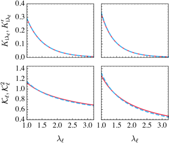
Figure 6: Comparison of asymptotic approximations (dashed blue) and exact functions (solid red); top-right $\displaystyle K_{\text{i}\lambda_{\ell}}$, top-left $\displaystyle K_{\text{i}\lambda_{\ell}}^{\prime}$, bottom-right $\displaystyle\mathcal{K}_{\ell}$ and bottom-left $\displaystyle\mathcal{K}_{\ell}^{2}$. The horizontal axis ranges within the interval (24) for $\displaystyle\lambda_{\ell}>1$, for each $\displaystyle\ell$.

Appendix C Onset of bound states

C.1 Nonexistence of bound states of angular momenta $\displaystyle\ell\geq\gamma_{\alpha}$

We show that whenever $\displaystyle\Delta_{\ell}=\gamma_{\alpha}-\ell\leq 0$, Eq. (23) has no solutions for $\displaystyle q$ real and positive.

We note that $\displaystyle K_{\nu}(x)$ of real order $\displaystyle\nu$ is a positive and decreasing function of $\displaystyle x\in]0,+\infty[$, hence we have

$$\left(\ln R_{2}\right)^{\prime}(r_{\alpha})=q\frac{K_{\nu}^{\prime}(qr_{\alpha})}{K_{\nu}(qr_{\alpha})}<0$$ (86)

for all $\displaystyle q>0$, where $\displaystyle\nu=\sqrt{\ell^{2}-\gamma_{\alpha}^{2}}$. It follows that solutions of (23) would require

$$\left(\ln R_{1}\right)^{\prime}(r_{\alpha})<0\,.$$ (87)

In turn, according to the properties of the CHF for positive parameters presented in Appendix A.1, it follows that

$$\displaystyle\left(\ln R_{1}\right)^{\prime}(r_{\alpha})=$$

$$\displaystyle=\frac{\left|\Delta_{\ell}\right|}{r_{\alpha}}+\frac{2\gamma_{\alpha}}{r_{\alpha}}\frac{M^{\prime}\left(\frac{1}{2}\left|\Delta_{\ell}\right|+\frac{q^{2}}{2\alpha\gamma}+\frac{1}{2},\ell+1;\gamma_{\alpha}\right)}{M\left(\frac{1}{2}\left|\Delta_{\ell}\right|+\frac{q^{2}}{2\alpha\gamma}+\frac{1}{2},\ell+1;\gamma_{\alpha}\right)}>0$$ (88)

for $\displaystyle q>0$. We conclude that Eq. (87) is not satisfied and that Eq. (23) has no solutions for $\displaystyle q>0$, implying that there are no bound states of angular momenta $\displaystyle\ell\geq\gamma_{\alpha}$.

C.2 Onset of bound states in finite size

C.2.1 Case $\displaystyle p=0$

Although (41) has, in general, no closed form solution, we can obtain an approximate solution for the state $\displaystyle p=0$ of each angular momentum $\displaystyle\ell$, since the onset of that state will take place for small values of $\displaystyle\lambda_{\ell}$ whenever $\displaystyle R\gg\xi$. We may thus solve

$$\Lambda_{\ell*}=\frac{\xi}{\alpha R}$$ (89)

to leading order in $\displaystyle\lambda_{\ell}$, with $\displaystyle\Lambda_{\ell*}\equiv\Lambda_{\ell}(\lambda_{\ell*})$ the function given by Eq. (29)

The function $\displaystyle\theta_{\ell}$ specified in Eq. (27) can be Taylor-expanded around $\displaystyle\lambda_{\ell}\geq 0$ to leading order as

$$\theta_{\ell}=\begin{cases}\frac{\pi}{2}-\gamma_{\alpha}+\mathcal{O}(\gamma_{\alpha}^{2})&,\,\ell=0\\ -a_{\ell}\lambda_{\ell}+\mathcal{O}(\lambda_{\ell}^{3})&,\,\ell\geq 1\end{cases}\,,$$

with

$$a_{\ell}=\left(1+\frac{1}{\ell}\right)\frac{M\left(\frac{1}{2},\ell+1;\ell\right)}{M\left(\frac{3}{2},\ell+2;\ell\right)}\,,$$

by virtue of the derivative of the CHF satisfying Olver et al. (2010)

$$M^{\prime}(a,b;z)=\frac{a}{b}M(a+1,b+1;z)\,.$$

Note that, for $\displaystyle\ell\geq 1$, we must first express $\displaystyle\gamma_{\alpha}$ to leading order in $\displaystyle\lambda_{\ell}$, given by $\displaystyle\gamma_{\alpha}=\ell+\lambda_{\ell}^{2}/(2\ell)+\mathcal{O}(\lambda_{\ell}^{4})$. In turn, Eq. (61) gives $\displaystyle\varphi_{\ell}=-\gamma_{\text{E}}\lambda_{\ell}+\mathcal{O}(\lambda_{\ell}^{3})$ to leading order in $\displaystyle\lambda_{\ell}$.

We begin with the case $\displaystyle\ell\geq 1$. Eq. (89) becomes, to leading order in $\displaystyle\lambda_{\ell}$,

$$\frac{\sqrt{2}}{\ell}\exp\left(-\frac{\pi}{\lambda_{\ell*}}\right)e^{a_{\ell}-\gamma_{E}}=\frac{\xi}{\alpha R}\,,$$

which can be rearranged to yield

$$\lambda_{\ell*}=\frac{\pi}{\log\left(\frac{R}{\xi r_{0,\ell}}\right)}\left(1+\mathcal{O}(\lambda_{\ell*}^{2})\right)\,,$$

with $\displaystyle r_{p=0,\ell}=e^{\gamma_{\text{E}}-a_{\ell}}\sqrt{3\ell^{2}/5}$. Squaring this result, Eq. (41) yields

$$\frac{g_{12}m_{2}}{g_{11}m_{1}}>\alpha^{2}\ell^{2}+\frac{c_{0,\ell}^{-2}}{\log\left(\frac{R}{\xi r_{0,\ell}}\right)^{2}}\,,$$ (90)

with $\displaystyle c_{p=0,\ell}=\pi^{-1}\sqrt{6/5}$. Higher-order terms in $\displaystyle\log\left(R/r_{0,\ell}\right)^{-1}$ can be obtained by expanding $\displaystyle\theta_{\ell}$, $\displaystyle\varphi_{\ell}$ and $\displaystyle\gamma_{\alpha}$ to subleading order in $\displaystyle\lambda_{\ell}$, but these are found to be negligible.

Table 1: Results of the fits (96) to the data from (95) for values of $\displaystyle c_{p,\ell}$ (top) and $\displaystyle\ln(1/r_{p,\ell})$ (bottom).

$\displaystyle p$	$\displaystyle 0$	$\displaystyle 1$	$\displaystyle 2$	$\displaystyle 3$	$\displaystyle 4$
$\displaystyle\>\ell=0$	0.7251	0.2365	0.1357	0.0932	0.0706
	1.0826	0.2642	0.2493	0.4039	0.5555
$\displaystyle\>\ell=1$	0.3248	0.1674	0.1130	0.0843	0.0663
	1.0191	0.6487	0.4144	0.3376	0.3721
$\displaystyle\>\ell=2$	0.3133	0.1554	0.1042	0.0786	0.0629
	0.1441	0.2474	0.2653	0.2562	0.2713

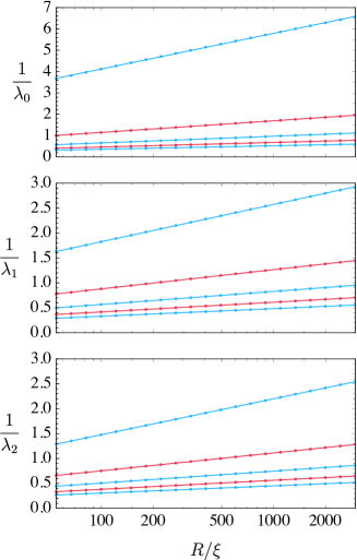
Figure 7: (color online) Comparisons of the fits (96) to the data from (95) for $\displaystyle\ell=0$ (top), $\displaystyle\ell=1$ (middle) and $\displaystyle\ell=2$ (bottom), for $\displaystyle p=0,1,2,3,4$ in descending order on the plots for each $\displaystyle\ell$. The horizontal axis $\displaystyle R/\xi$ is in logarithmic scale.

For the case $\displaystyle\ell=0$, we may take Eq. (89) to leading order in $\displaystyle\gamma_{\alpha}$ and rearrange it as

$$\gamma_{\alpha*}=\frac{3\pi}{2}\frac{1}{1-\gamma_{E}-\log\frac{\xi\gamma_{\alpha*}}{\sqrt{2}\alpha R}}\,.$$ (91)

We note that for $\displaystyle R\gg\xi$, the RHS of (LABEL:eq:sat-electable) depends very weakly on $\displaystyle\gamma_{\alpha*}$; indeed, numerical evidence indicates that the solution $\displaystyle\gamma_{\alpha*}=\gamma_{\alpha*}(R)$, for each $\displaystyle R$, is well approximated to zeroth order in $\displaystyle R$ by $\displaystyle\gamma_{\alpha*}(R)\approx\gamma_{\text{E}}$ over a range $\displaystyle 200<R/\xi<2000$ . Then, we may write $\displaystyle\gamma_{\alpha*}=\gamma_{\text{E}}+\gamma_{\text{E}}\delta_{*}$, with $\displaystyle\delta_{*}=\gamma_{\alpha}/\gamma_{\text{E}}-1\ll 1$ small, by hypothesis, so that we can take (91) to leading order in $\displaystyle\delta_{*}$ to yield

$$\gamma_{\alpha*}=\frac{\frac{3\pi}{2}-\gamma_{\text{E}}}{\log\left(\frac{R}{\xi r_{0,0}}\right)}\,,$$ (92)

with $\displaystyle r_{0,0}=e^{\gamma_{\text{E}}}\sqrt{3\gamma_{\text{E}}^{2}/5}$. Finally, squaring this result, Eq. (41) yields

$$\frac{g_{12}m_{2}}{g_{11}m_{1}}>\frac{c_{0,0}^{-2}}{\log\left(\frac{R}{\xi r_{0,0}}\right)^{2}}\,,$$ (93)

with $\displaystyle c_{0,0}=\left(3\pi/2-\gamma_{\text{E}}\right)^{-1}\sqrt{6/5}$. These results suggest we can establish a law

$$\frac{g_{12}m_{2}}{g_{11}m_{1}}>\alpha^{2}\ell^{2}+\frac{c_{0,\ell}^{2}}{\log\left(\frac{R}{\xi r_{0,\ell}}\right)^{2}}\,,$$ (94)

valid, at least, for $\displaystyle p=0$.

C.2.2 Case $\displaystyle p\geq 0$

In general, the foregoing considerations in the derivations of (90) and (93) no longer hold. However, we can show that condition (94) is accurate as well for $\displaystyle p\geq 1$: we obtain numerical solutions of Eq. (89) over a range $\displaystyle 50<R/\xi<3000$, by employing a Newton method to the equation

$$\ln\Lambda_{\ell*}=-\ln\frac{\alpha R}{\xi}\,;$$ (95)

we then perform a linear fit of the expression on the RHS of (94) to parameters $\displaystyle c_{p,\ell}$ and $\displaystyle r_{p,\ell}$ in a $\displaystyle 1/\lambda_{\ell}$ vs. $\displaystyle\ln(R/\xi)$ plot, i.e.

$$\frac{1}{\lambda_{\ell}}=c_{p,\ell}\left(\ln\frac{R}{\xi}-\ln r_{p,\ell}\right)\,.$$ (96)

Graphical comparisons are in displayed in Fig. 7, while results of the fit are given in Table. 1 for a few bound states. We thus conclude that Eq. (42) provides a condition for the onset of any bound state $\displaystyle(p,\ell)$.

References

- Gordon and Shestakov (2000) E. B. Gordon and A. F. Shestakov, Low Temperature Physics 26, 1 (2000).
- Devreese (2014) J. T. Devreese, Physics Today 67, 54 (2014).
- Dykman and Rashba (2015) M. I. Dykman and E. I. Rashba, Physics Today 68, 10 (2015).
- Vojta (2019) T. Vojta, Annual Review of Condensed Matter Physics 10, 233 (2019).
- Devreese (2003) J. T. Devreese, “Polarons,” in digital Encyclopedia of Applied Physics (American Cancer Society, 2003).
- Drescher et al. (2019) M. Drescher, M. Salmhofer, and T. Enss, Phys. Rev. A 99, 023601 (2019).
- Yoshida et al. (2018) S. M. Yoshida, S. Endo, J. Levinsen, and M. M. Parish, Phys. Rev. X 8, 011024 (2018).
- Fröhlich et al. (1950) H. Fröhlich, H. Pelzer, and S. Zienau, The London, Edinburgh, and Dublin Philosophical Magazine and Journal of Science 41, 221 (1950).
- Grimvall (1981) G. Grimvall, The Electron-Phonon Interaction in Metals (Selected Topics in Solid State Physics XVI) (North-Holland Pub. Co. : sole distributors for the U.S.A. and Canada, Elsevier North-Holland, 1981).
- Stamatis (1995) D. Stamatis, Understanding ISO 9000 and Implementing the Basics to Quality (Quality and Reliability) (CRC Press, 1995).
- Swartz et al. (2018) A. G. Swartz, H. Inoue, T. A. Merz, Y. Hikita, S. Raghu, T. P. Devereaux, S. Johnston, and H. Y. Hwang, Proceedings of the National Academy of Sciences 115, 1475 (2018), https://www.pnas.org/content/115/7/1475.full.pdf .
- Appel (1969) J. Appel, Phys. Rev. 180, 508 (1969).
- Gerlach and Löwen (1991) B. Gerlach and H. Löwen, Rev. Mod. Phys. 63, 63 (1991).
- Kudinov (2002) E. K. Kudinov, Physics of the Solid State 44, 692 (2002).
- Grimaldi (2008) C. Grimaldi, Phys. Rev. B 77, 024306 (2008).
- Grimaldi (2010) C. Grimaldi, Phys. Rev. B 81, 075306 (2010).
- Frank and Schlein (2014) R. L. Frank and B. Schlein, Letters in Mathematical Physics 104, 911 (2014).
- Tempere et al. (2009) J. Tempere, W. Casteels, M. K. Oberthaler, S. Knoop, E. Timmermans, and J. T. Devreese, Phys. Rev. B 80, 184504 (2009).
- Catani et al. (2012) J. Catani, G. Lamporesi, D. Naik, M. Gring, M. Inguscio, F. Minardi, A. Kantian, and T. Giamarchi, Phys. Rev. A 85, 023623 (2012).
- Scelle et al. (2013) R. Scelle, T. Rentrop, A. Trautmann, T. Schuster, and M. K. Oberthaler, Phys. Rev. Lett. 111, 070401 (2013).
- Jørgensen et al. (2016) N. B. Jørgensen, L. Wacker, K. T. Skalmstang, M. M. Parish, J. Levinsen, R. S. Christensen, G. M. Bruun, and J. J. Arlt, Phys. Rev. Lett. 117, 055302 (2016).
- Mistakidis et al. (2019) S. I. Mistakidis, G. C. Katsimiga, G. M. Koutentakis, T. Busch, and P. Schmelcher, Phys. Rev. Lett. 122, 183001 (2019).
- Peña Ardila et al. (2019) L. A. Peña Ardila, N. B. Jørgensen, T. Pohl, S. Giorgini, G. M. Bruun, and J. J. Arlt, Phys. Rev. A 99, 063607 (2019).
- Pelmenev et al. (2016) A. A. Pelmenev, I. N. Krushinskaya, I. B. Bykhalo, and R. E. Boltnev, Low Temperature Physics 42, 224 (2016).
- Barenghi et al. (2014) C. F. Barenghi, L. Skrbek, and K. R. Sreenivasan, Proceedings of the National Academy of Sciences 111, 4647 (2014).
- Escartín et al. (2019) J. M. Escartín, F. Ancilotto, M. Barranco, and M. Pi, Phys. Rev. B 99, 140505 (2019).
- Pshenichnyuk (2017) I. A. Pshenichnyuk, New Journal of Physics, 19, 105007 (2017).
- Abo-Shaeer et al. (2001) J. R. Abo-Shaeer, C. Raman, J. M. Vogels, and W. Ketterle, Science 292, 476 (2001).
- Lin et al. (2009) Y.-J. Lin, R. L. Compton, K. Jiménez-García, J. V. Porto, and I. B. Spielman, Nature 462, 628 (2009).
- Madison et al. (2000) K. W. Madison, F. Chevy, W. Wohlleben, and J. Dalibard, Physical Review Letters 84, 806 (2000).
- Matthews et al. (1999) M. R. Matthews, B. P. Anderson, P. C. Haljan, D. S. Hall, C. E. Wieman, and E. A. Cornell, Physical Review Letters 83, 2498 (1999).
- Andersen et al. (2006) M. F. Andersen, C. Ryu, P. Cladé, V. Natarajan, A. Vaziri, K. Helmerson, and W. D. Phillips, Phys. Rev. Lett. 97, 170406 (2006).
- Schweikhard et al. (2004) V. Schweikhard, I. Coddington, P. Engels, V. P. Mogendorff, and E. A. Cornell, Physical Review Letters 92 (2004), 10.1103/physrevlett.92.040404.
- Svidzinsky and Fetter (2000) A. A. Svidzinsky and A. L. Fetter, Phys. Rev. Lett. 84, 5919 (2000).
- Shaukat et al. (2017) M. I. Shaukat, E. V. Castro, and H. Terças, Physical Review A 95, 053618 (2017).
- Shaukat et al. (2018) M. I. Shaukat, E. V. Castro, and H. Terças, Physical Review A 98, 022319 (2018).
- Shaukat et al. (2019) M. I. Shaukat, E. V. Castro, and H. Terças, Physical Review A 99, 042326 (2019).
- Pitaevskii and Stringari (2003) L. Pitaevskii and S. Stringari, Bose-Einstein Condensation (International Series of Monographs on Physics) (Clarendon Press, 2003).
- Pethick and Smith (2008) C. J. Pethick and H. Smith, Bose–Einstein Condensation in Dilute Gases, 2nd ed. (Cambridge University Press, 2008).
- Kawaguchi and Ohmi (2004) Y. Kawaguchi and T. Ohmi, Phys. Rev. A 70, 043610 (2004).
- Cidrim et al. (2017) A. Cidrim, A. C. White, A. J. Allen, V. S. Bagnato, and C. F. Barenghi, Phys. Rev. A 96, 023617 (2017).
- Manton and Sutcliffe (2004) N. Manton and P. Sutcliffe, Cambridge Monographs on Mathematical Physics (Cambridge University Press, Cambridge, 2004).
- Konishi and Paffuti (2009) K. Konishi and G. . . Paffuti, Quantum mechanics: a new introduction (Oxford University Press, 2009).
- Olver et al. (2010) F. W. Olver, D. W. Lozier, R. F. Boisvert, and C. W. Clark, NIST Handbook of Mathematical Functions, 1st ed. (Cambridge University Press, New York, NY, USA, 2010).
- Dunster (1990) T. M. Dunster, SIAM Journal on Mathematical Analysis, SIAM Journal on Mathematical Analysis 21, 995 (1990).
- Lundh et al. (1998) E. Lundh, C. J. Pethick, and H. Smith, Physical Review A 58, 4816 (1998).
- Schäfer et al. (2018) F. Schäfer, N. Mizukami, P. Yu, S. Koibuchi, A. Bouscal, and Y. Takahashi, Physical Review A 98, 051602 (2018).
- Gross and Khaykovich (2008) N. Gross and L. Khaykovich, Physical Review A 77, 023604 (2008).
- Salasnich et al. (2002) L. Salasnich, A. Parola, and L. Reatto, Phys. Rev. A 65, 043614 (2002).
- Krüger et al. (2007) P. Krüger, Z. Hadzibabic, and J. Dalibard, Phys. Rev. Lett. 99, 040402 (2007).
- Young-S. et al. (2010) L. E. Young-S., L. Salasnich, and S. K. Adhikari, Phys. Rev. A 82, 053601 (2010).
- Zhang et al. (2008) W. Zhang, G.-D. Lin, and L.-M. Duan, Phys. Rev. A 78, 043617 (2008).
- Gaunt et al. (2013) A. L. Gaunt, T. F. Schmidutz, I. Gotlibovych, R. P. Smith, and Z. Hadzibabic, Phys. Rev. Lett. 110, 200406 (2013).
- Gotlibovych et al. (2014) I. Gotlibovych, T. F. Schmidutz, A. L. Gaunt, N. Navon, R. P. Smith, and Z. Hadzibabic, Phys. Rev. A 89, 061604 (2014).
- Chomaz et al. (2015) L. Chomaz, L. Corman, T. Bienaimé, R. Desbuquois, C. Weitenberg, S. Nascimbène, J. Beugnon, and J. Dalibard, Nature Communications 6, 6162 (2015).
- Desbuquois et al. (2014) R. Desbuquois, T. Yefsah, L. Chomaz, C. Weitenberg, L. Corman, S. Nascimbène, and J. Dalibard, Phys. Rev. Lett. 113, 020404 (2014).
- Essin and Griffiths (2006) A. M. Essin and D. J. Griffiths, American Journal of Physics, American Journal of Physics 74, 109 (2006).
- Catelani and Yuzbashyan (2010) G. Catelani and E. A. Yuzbashyan, Physical Review A 81, 033629 (2010).
- Hansen et al. (2013) A. H. Hansen, A. Y. Khramov, W. H. Dowd, A. O. Jamison, B. Plotkin-Swing, R. J. Roy, and S. Gupta, Phys. Rev. A 87, 013615 (2013).
- Khramov et al. (2014) A. Khramov, A. Hansen, W. Dowd, R. J. Roy, C. Makrides, A. Petrov, S. Kotochigova, and S. Gupta, Phys. Rev. Lett. 112, 033201 (2014).
- Caracanhas et al. (2013) M. A. Caracanhas, V. S. Bagnato, and R. G. Pereira, Phys. Rev. Lett. 111, 115304 (2013).
- Ancarani and Gasaneo (2008) L. U. Ancarani and G. Gasaneo, Journal of Mathematical Physics, Journal of Mathematical Physics 49, 063508 (2008).
- foo (a) In the present work, we avoid the usual notation for the incomplete gamma function as to avoid any ambiguities with the parameter . (a).
- Olver (1997) F. W. Olver, Asymptotics and Special Functions, 1st ed. (A K Peters/CRC, New York, NY, USA, 1997).
- Jeffrey and Zwillinger (2007) A. Jeffrey and D. Zwillinger, Table of Integrals, Series, and Products (Elsevier Science, 2007).
- foo (b) We disregard the condition by the convergence argument presented following Eq. (76) and due to the fact that the integral in Eq. (81) exists formally even for . (b).
- Magnus et al. (2013) W. Magnus, F. Oberhettinger, and R. Soni, Formulas and Theorems for the Special Functions of Mathematical Physics (Springer Berlin Heidelberg, 2013).