Monte-Carlo simulations of relativistic radiation mediated shocks: II. photon starved regime

Abstract

Radiation mediated shocks (RMS) play a key role in shaping the early emission observed in many transients. In most cases, e.g., shock breakout in supernovae, llGRBs and neutron star mergers, the upstream plasma is devoid of radiation, and the photons that ultimately reach the observer are generated predominantly inside and downstream of the shock. Predicting the observed spectrum requires detailed calculations of the shock structure and thermodynamic state that account properly for the shock microphysics. We present results of self-consistent Monte-Carlo simulations of photon-starved RMS, that yield the shock structure and emission for a broad range of shock velocities, from sub-relativistic ($\beta_{sh}=0.1$) to highly relativistic ($\Gamma_{sh}=20$). Our simulations confirm that in relativistic RMS the immediate downstream temperature is regulated by exponential pair creation, ranging from $50$ keV at $\beta_{sh}=0.5$ to $200$ keV at $\Gamma_{sh}=20$. At lower velocities the temperature becomes sensitive to the shock velocity, with $kT\sim 0.5$ keV at $\beta_{sh}=0.1$. We also confirm that in relativistic shocks the opacity is completely dominated by newly created pairs, which has important implications for the breakout physics. We find the transition to pair dominance to occur at $\beta_{sh}=0.5$ roughly. In all cases examined, the spectrum below the $\nu F_{\nu}$ peak has been found to be substantially softer than the Planck distribution. This has important implications for the optical emission in fast and relativistic breakouts, and their detection. The applications to GRB 060218 and GRB 170817A are discussed.

1 Introduction

The early emission observed in various types of cosmic explosions is released during the breakout of a radiation mediated shock (RMS) from the envelope enshrouding the blast center (for a recent review, see Levinson & Nakar, 2019). In such shocks the dissipation mechanism involves emission and scattering of radiation and, under certain conditions, pair production. The properties of the breakout signal and the subsequent cooling envelope emission depend on the shock velocity and structure, as well as on the upstream conditions. The shock velocity during the breakout phase can range from subrelativistic in regular supernovae, through mildly relativistic in, e.g., long gamma-ray bursts (LGRBs) and neutron star (NS) mergers, to highly relativistic in energetic aspherical explosions of compact progenitors (Nakar & Sari, 2012).

Two disparate regimes have been identified (Levinson & Nakar, 2019); photon rich shocks in which advection of upstream radiation determines the downstream state, and photon starved shocks in which photons are generated predominantly inside and just downstream of the shock transition layer. The former case is anticipated in sub-photospheric shocks in GRBs (Levinson & Bromberg, 2008; Levinson, 2012; Beloborodov, 2017; Lundman, Beloborodov & Vurm, 2018; Ito et al., 2018), whereas the latter in most other systems (Weaver, 1976; Katz, Budnik, & Waxman, 2010; Budnik et al., 2010; Nakar & Sari, 2010, 2012; Granot, Nakar & Levinson, 2018; Ioka, Levinson & Nakar, 2019). In a previous paper (Ito et al., 2018, hereafter paper I) we presented a comprehensive analysis of photon rich RMS and its application to LGRBs, using a Monte-Carlo method that solves the shock structure coupled to the transfer of radiation through the shock in a self-consistent manner. We have shown that photon advection dominates over photon generation when the photon-to-baryon ratio far upstream exceeds the e-p mass ratio times the shock Lorentz factor, and that this ratio determines the immediate downstream temperature. We have also shown that the observed spectrum is expected to be broad owing to bulk comptonization. Similar results were obtained by Beloborodov (2017) and Lundman, Beloborodov & Vurm (2018) using a different method, verifying the validity of the two techniques.

In this paper we use a modified version of our Monte-Carlo code (see Appendix A for details), that includes photon generation and absorption in addition to scattering and pair creation, to compute the structure and spectrum of photon starved shocks for a broad range of shock velocities, from $\beta_{u}=0.1$ up to $\Gamma_{u}=20$, where $\beta_{u}$ is the velocity of the upstream plasma, as measured in the shock frame, and $\Gamma_{u}$ is the corresponding Lorentz factor.

In general, photon starved RMS exhibit three different velocity domains with vastly different behaviours (Katz, Budnik, & Waxman, 2010; Levinson & Nakar, 2019): (i) Slow shocks ($\beta_{u}<0.05$) in which the radiation is in full thermodynamic equilibrium already inside the shock transition layer, and the temperature depends weakly on shock velocity and plasma density. In such shocks the emitted spectrum is a black body spectrum. (ii) Fast Newtonian shocks ($0.05\lesssim\beta_{u}\lesssim 0.5$), in which the radiation is out of thermodynamic equilibrium, and the temperature is determined by the photon generation rate in the immediate downstream, and depends very sensitively on shock velocity. (iii) Relativistic shocks in which pair creation and Klein-Nishina effects play a dominant role. Relativistic RMS have been thoroughly analyzed in the highly relativistic regime ($\Gamma_{u}\geq 6$) by Budnik et al. (2010), using a kinetic approach to solve the radiative transfer equation inside the shock. Our analysis, that exploits a different technique, confirms those previous results, and is extended to the fast Newtonian and mildly relativistic regimes that apply to the majority of strong stellar explosions, allowing, for the first time, to perform self-consistent calculations of the RMS structure and inherent spectrum in these cases, which is the prime goal of this study. The shock structure computed in our simulations is found to be in good agreement with semi-analytic solutions obtained both in the Newtonian limit (Blandford & Payne, 1981b; Ioka, Levinson & Nakar, 2019) and in the highly relativistic limit (Nakar & Sari 2012; Granot, Nakar & Levinson 2018 hereafter GNL18). More importantly, we find that in fast Newtonian and relativistic RMS the spectrum during shock breakout (and conceivably the early cooling emission) deviates considerably from a black body, which has important implications for the detection of these sources.

This paper is organized as follows. In Section 2 we describe the numerical method and the setup of our simulations. We present the main results in Section 3. In Section 4 we discuss the applications to shock breakouts, with particular attention to GRB 060218 and GRB 170817A. We conclude in Section 5. Throughout the paper, the subscript $u$ and $d$ refer to the physical quantities at the far upstream and far downstream regions of the shock, respectively.

2 Numerical Setup

The Monte-Carlo RMS code which we have developed enables us to compute the steady-state profile of RMS for a range of shock velocities that encompasses the sub-relativistic and ultra-relativistic regimes. The code iteratively seeks a self-consistent flow profile that satisfies energy-momentum conservation at all grid points. More precisely, under the assumption that protons and pairs each have a local Maxwellian distribution with the same temperature, we compute the transfer of radiation through the shock for the given plasma profile using Monte-Carlo techniques. Based on the departure from the energy-momentum conservation evaluated in each cycle, the shock profile is modified iteratively until convergence is reached to the desired accuracy. The details are described in Paper I for photon rich RMS. The main modification in the present analysis is the inclusion of free-free emission/absorption processes which are essential in photon starved shocks. A summary of the updates is outlined in Appendix A.

In the current study, the input parameters are the 4-velocity of the upstream flow, $\Gamma_{\rm u}\beta_{\rm u}$, the proper baryon density at the far upstream region $n_{\rm u}$, and the composition, which we take to be purely hydrogen. As for the baryon density, we invoke a fixed value of $n_{\rm u}=10^{15}~{}{\rm cm}^{-3}$ which is identical to that adopted in the calculations of Budnik et al. (2010). It is worth noting that the solutions are not sensitive to the choice of $n_{\rm u}$; in the fully and mildly relativistic regimes the immediate downstream temperature is always around $\sim 100-200~{}{\rm keV}$, owing to the pair creation thermostat (see Budnik et al., 2010, and next section). Even in the sub-relativistic regime the dependence of the temperature on $n_{\rm u}$ is only mild (but might be important from an observational perspective, see Levinson & Nakar, 2019, for discussion). The composition can alter the downstream temperature if heavy and in particular in case of r-process material (see Fig. 15 in Levinson & Nakar, 2019); we leave the investigation of composition effects, that are mainly relevant to NS mergers, for a future work.

As stated in the introduction, we are interested in exploring the regimes of fast Newtonian and relativistic shocks ($\beta_{\rm u}>0.05$). To that end we consider 6 models with different values of the upstream 4-velocity, which translate to $\beta_{\rm u}=0.1$, $0.5$, and $\Gamma_{\rm u}=2$, $6$, $10$ and $20$. The Lorentz factors in the highly relativistic regime ($\Gamma_{\rm u}=6,10,20$) were chosen to enable a direct comparison with the results of Budnik et al. (2010). As for the remaining cases, to our knowledge this is the first time ever that ab-initio calculations of RMS in those regimes have been performed.

As described in Appendix B, we inject a minuet amount of thermal photons at the upstream boundary merely for numerical convenience. This has no practical effect on the solutions, since the new photons generated by free-free emission dominate the radiation field already in the far upstream. To confirm this, we checked that the results converge by changing the density and energy of the injected photon population.

3 Results

3.1 Overall structure

Fig. 1 shows the profiles of the 4-velocity, temperature, pair-to-baryon ratio and photon-to-baryon ratio, plotted as functions of the angle averaged, pair loaded Thomson optical depth, $\tau_{*}=\int\Gamma(n+n_{\pm})\sigma_{T}dx$, where $n_{\pm}$ is the pair density and $\sigma_{T}$ is the Thomson cross section. A zoom in of the immediate downstream region is shown in Fig. 2 for the relativistic shocks. It indicates formation of subshocks, as also found in Budnik et al. (2010). While non negligible, they do not alter significantly the overall shock structure. We shall discuss them in greater detail below. Such subshocks are absent in the fast Newtonian regime ($\Gamma_{\rm u}\beta_{\rm u}<1$).

Fig. 1 confirms that the transition from the fast Newtonian regime to the relativistic regime occurs at $\beta_{\rm u}\simeq 0.5$. The temperature just behind the shock changes from about $0.5$ keV at $\beta_{\rm u}=0.1$ to about $50$ keV at $\beta_{\rm u}=0.5$, confirming the sensitive dependence found earlier analytically (Weaver, 1976; Katz, Budnik, & Waxman, 2010). At $\beta_{\rm u}=0.1$ the simulation result is in excellent agreement with the analytic estimates, as can be seen by comparing the value found in our simulation with Fig 5 in Levinson & Nakar (2019). At $\beta_{\rm u}>0.5$ there is only a very weak dependence of the temperature on $\Gamma_{\rm u}\beta_{\rm u}$, owing to the exponential pair creation thermostat mentioned above. The rapid increase of the pair content with increasing $\Gamma_{\rm u}\beta_{\rm u}$ is clearly seen in the bottom panel of Fig. 1 for $\beta_{\rm u}>0.5$. At lower velocities the $n_{\pm}/n$ ratio is found to be practically zero. The photon generation along the flow results in a significant increase in the photon number towards downstream. As seen in the figure, emergence of copious pairs for $\beta_{\rm u}\geq 0.5$ largely enhances the photon production. It is noted that the discontinuous change of photon to baryon ratio at $\tau_{*}=0$ for $\Gamma_{\rm u}\geq 2$ is due to the instantaneous change in the inertial frame as well as the comoving baryon density across the subshock.

As also seen, the shock width increases with decreasing velocity in the Newtonian regime, whereas it increases with increasing Lorentz factor in the relativistic regime. As will be discussed in more detail in Section 3.1.2 below, the reason for this apparently peculiar behaviour is that in the Newtonian regime the width is set by the diffusion length of photons, whereas in the relativistic regime it is largely affected by Klien-Nishina suppression. This suppression allows photons that propagate from the downstream to the upstream to penetrate to a much larger distances ahead of the shock and, as a result, a substantial increase in the temperature and pair density begins well before the flow decelerates, at increasingly larger distance for larger $\Gamma_{\rm u}$. The maximal value of the temperature is attained at the upstream, while the pairs density reaches its maximum in the near downstream (Fig. 2). A quantitative scaling of the physical shock width across the entire velocity range is derived in Section 3.1.2 below.

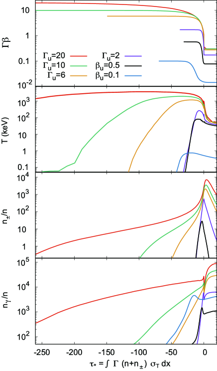
Figure 1: Overall shock structure for upstream velocities of $\beta_{\rm u}=0.1$ (blue), $\beta_{\rm u}=0.5$ (black), $\Gamma_{\rm u}=2$ (magenta), $\Gamma_{\rm u}=6$ (brown), $\Gamma_{\rm u}=10$ (green) and $\Gamma_{\rm u}=20$ (red). In each panel, from top to bottom, we display the 4-velocity $\Gamma\beta$, the plasma temperature $T$, the pair -to- baryon density ratio $n_{\pm}/n$ and the photon -to- baryon ratio $n_{\gamma}/n$, as a function of optical depth $\tau_{*}$. The location of $\tau_{*}=0$ are taken at the position of the subshock ($\Gamma_{\rm u}\geq 2$) or the position where the velocity satisties $\beta=1.05\beta_{\rm d}$ when subshock is absent ($\beta_{\rm u}\leq 0.5$).

3.1.1 Subshocks

As mentioned above, one of the characteristic features which is only seen in relativistic RMS is formation of a subshock. Our simulations indicate that, while the photon-plasma interaction leads to a smooth transition at $\beta_{\rm u}\lesssim 0.5$, subshocks inevitably form when $\Gamma_{\rm u}\gtrsim 2$. A similar phenomena was found also in photon rich shocks, although the subshocks there are much weaker (paper I). A close-up view of the subshock region is shown in Fig. 2. It is overall consistent with the substructures seen in the simulations of Budnik et al. (2010), however, the strength of the subshocks in our simulations are larger than those reported in Budnik et al. (2010). The velocity jump across the subshock they find is roughly $\delta(\Gamma\beta)\sim 0.1$ for all the cases they explored ($\Gamma_{\rm u}=6,10,20$ and $30$), implying negligible energy dissipation, whereas we find velocity jumps of $\delta(\Gamma\beta)\sim 0.16$, $0.33$, $0.38$ and $0.66$ for $\Gamma_{\rm u}=2$, $6$, $10$ and $20$, respectively, with subshock dissipation of a few percents of the total shock energy The origin of this discrepancy may be traced to the approximation imposed in their analysis. A careful scrutiny of their analysis can be found in Appendix E. Apart from these details, our simulations show a broad agreement with Budnik et al. (2010), as will be discussed further below.

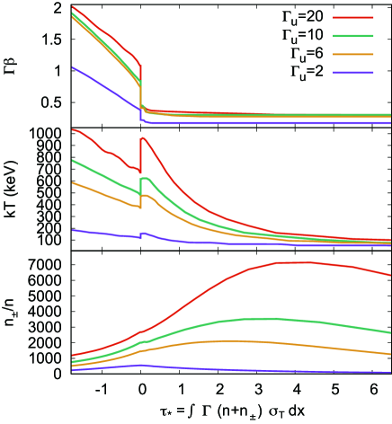
Figure 2: Enlarged view of the 4-velocity (top), temperature (middle) and pair -to- baryon ratio (bottom) near the subshock for upstream Lorentz factors of $\Gamma_{\rm u}=2$ (magenta), $\Gamma_{\rm u}=6$ (brown), $\Gamma_{\rm u}=10$ (green) and $\Gamma_{\rm u}=20$ (red).

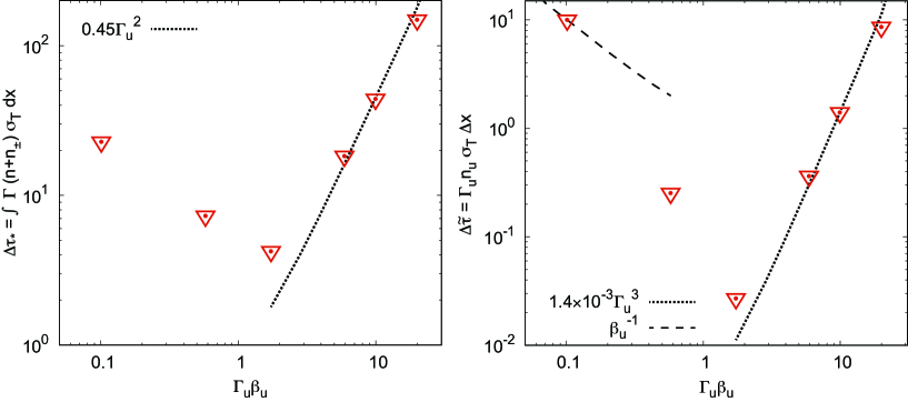
Figure 3: Pair loaded Thomson optical depth (left) and dimensionless width (right) of the shock transition layer. Here the shock width $\Delta x$, as measured in the shock frame, is defined as the distance from the location where $(\Gamma\beta)/(\Gamma_{\rm u}\beta_{\rm u})=0.9$ to the subshock, or to the downstream point where $(\Gamma\beta)/(\Gamma_{\rm d}\beta_{\rm d})=1.1$ when a subshock is absent. The red triangles show the results obtained from the simulations. The dotted and dashed lines delineate the scaling anticipated in the highly relativistic ( $\Delta\tau_{*}\propto\Gamma_{\rm u}^{2}$ and $\Delta\tilde{\tau}\propto\Gamma_{\rm u}^{3}$) and subrelativistic ($\Delta\tilde{\tau}\propto\beta_{\rm u}^{-1}$) regimes, respectively.

3.1.2 Scaling of the shock width

As stated above, the width of the shock transition layer (i.e., the deceleration zone) is a non-monotonic function of the shock 4-velocity. In the non-relativistic regime ($\beta_{\rm u}\ll 1$) the transport of radiation across the shock is diffusive, and the transition occurs rather gradually over one diffusion length roughly (Weaver, 1976; Blandford & Payne, 1981a, b; Katz, Budnik, & Waxman, 2010). By equating the diffusion time across the shock, $t_{D}=\Delta\tau_{*}L_{s}/c$, here $L_{s}$ is the shock width and $\Delta\tau_{*}=\int_{-L_{s}}^{0}\sigma_{T}ndx$ is the optical thickness of the shock, with the flow time, $t_{f}=\int_{-L_{s}}^{0}dx/c\beta=\Delta\tau_{*}/(\sigma_{T}n_{\rm u}\beta_{\rm u})$ (recalling that $n\beta=n_{\rm u}\beta_{\rm u}$), one obtains:

$$\sigma_{T}n_{\rm u}L_{s}\approx 1/\beta_{\rm u}.$$ (1)

The right panel in Fig. 3 shows good agreement between this naive estimate and the simulation result for $\beta_{\rm u}=0.1$ (see also Appendix C).

In difference, in the relativistic regime ($\beta_{\rm u}\sim 1$) counterstreaming photons are mostly scattered back in a single scattering. Nonetheless, the pair loaded Thomson optical depth is significantly larger than unity, and increases with increasing $\Gamma_{\rm u}$, by virtue of Klein-Nishina effects. In fact, the change of the shock width with $\Gamma_{\rm u}$ is nonlinear, since the temperature inside the shock is roughly proportional to the local Lorentz factor (Fig. 1), implying that the mean photon energy seen in the rest frame of an electron (or positron) and, hence, the Klein-Nishina suppression, scale as $\Gamma^{2}$. This heuristic result is in a good agreement with the simulations performed by Budnik et al. (2010) and the analytic solution derived in Nakar & Sari (2012) and GNL18, who find the scaling $\Delta\tau_{*}\propto\Gamma_{\rm u}^{2}$ (up to a logarithmic factor). These solutions also yield the scaling $\Delta\tilde{\tau}\propto\Gamma_{\rm u}^{3}$ for the pair unloaded depth of the shock transition layer, defined as $\Delta\tilde{\tau}=\int^{0}_{-\Delta x}\Gamma n\sigma_{T}dx=\sigma_{T}\Gamma_{\rm u}n_{\rm u}\Delta x$, where $\Delta x$ is the length, as measured in the shock frame, over which the shock Lorentz factor changes substantially (see GNL18 for details). The optical thickness $\Delta\tilde{\tau}$ corresponds to the minimum opacity needed to sustain the RMS; once the total optical depth ahead of the shock becomes smaller than this value, viz., $\tau\lesssim\Delta\tilde{\tau}$, radiation starts leaking out of the shock and the shock structure is significantly altered (GNL18). This is the point where breakout commences.

Fig. 3 shows the pair loaded Thomson depth of the shock transition layer $\Delta\tau_{*}$ (left panel), and the dimensionless shock width $\Gamma_{\rm u}n_{\rm u}\sigma_{T}\Delta x$ (right panel), measured in the simulations (the red triangles). The latter equals the pair unloaded Thomson optical depth in the limit $\Gamma_{\rm u}\gg 1$. The shock width $\Delta x$ is defined here as the backward distance (measured in the shock frame) from the subshock (or the point where $\Gamma\beta=1.1\Gamma_{\rm d}\beta_{\rm d}$ if there is no subshock), at which the 4-velocity reaches 90% of its upstream value, that is, $\Gamma(-\Delta x)\beta(-\Delta x)=0.9\Gamma_{\rm u}\beta_{\rm u}$. As seen, while for $\beta_{\rm u}=0.1$ the shock thickness $\Delta\tilde{\tau}$ agrees well with Eq. (1), it is much narrower for $\beta_{\rm u}=0.5$. The reason is that in this case the opacity inside the shock is dominated by newly created pairs, as can be inferred by comparing the results for $\beta_{\rm u}=0.5$ in the left and right panels. The simulation results also indicate that the scaling derived analytically in GNL18 and found numerically in Budnik et al. (2010) holds from $\Gamma_{\rm u}=6$ up to $\Gamma_{\rm u}=20$. At $\Gamma_{\rm u}=2$ we find somewhat departure from this scaling. This is expected since the scaling is valid in the relativitic limit.

The non-monotonic behaviour of the shock width implies that physical shock width ($\Delta x$ or equivalently $\Delta\tilde{\tau}$) has an absolute minimum. From our simulations we estimate that it occurs around $\Gamma_{\rm u}=2$ (see right panel in Fig. 3).

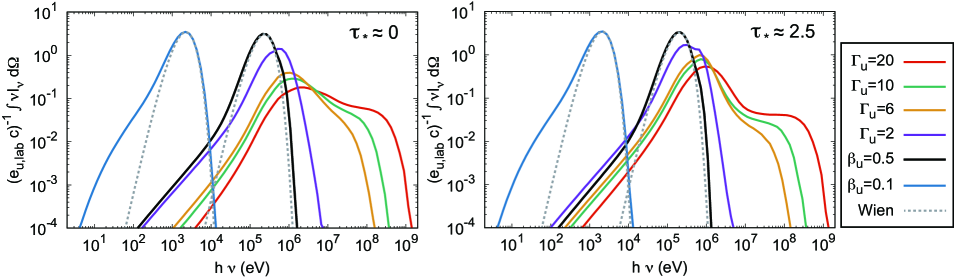
Figure 4: Shock-frame, local, angle integrated SEDs, $c^{-1}\int\nu I_{\nu}d\Omega$, normalized by the total kinetic energy density of the far upstream flow, $e_{\rm u}=\Gamma_{\rm u}(\Gamma_{\rm u}-1)n_{\rm u}m_{p}c^{2}$. The left and right panels correspond to the downstream locations $\tau_{*}\approx 0$ and $\tau_{*}\approx 2.5$, respectively. The blue, black, magenta, brown, green and red lines show the results for $\beta_{\rm u}=0.1$, $0.5$, and $\Gamma_{\rm u}=2$, $6$, $10$ and $20$, respectively. The dotted lines delineate the Wien spectra for the $\beta_{\rm u}=0.1$ and $\beta_{\rm u}=0.5$ cases.

3.2 Spectrum

Fig. 4 displays the angle-integrated spectral energy distribution (SED), as seen in the shock frame, at two locations in the immediate downstream, as indicated. (The angle dependent SED is shown for illustration in Fig. 5 for $\Gamma_{\rm u}=20$ at $\tau_{*}=2.5$.) All spectra exhibit substantial deviations from black body, as expected for fast RMS having $\beta_{\rm u}>0.05$ (see discussion above). The portion of the spectrum below the peak is much softer than that of a Planckian ($\nu I_{\nu}\propto\nu^{3}$) in all cases. It is produced by thermal Comptonization of soft photons that are continuously generated by bremsstrahlung emissions. The transition to the Planck regime occurs at a frequency (seen here only for $\beta_{\rm u}=0.1$) below which absorption becomes fast enough. This break frequency generally increases with decreasing downstream temperature (or shock velocity), and for the spectra exhibited in Fig. 4 is about $20$ eV for $\beta_{\rm u}=0.1$ and $1$ eV for $\beta_{\rm u}=0.5$. The overall spectrum slowly evolves towards a black body spectrum as the radiation is advected away from the shock, but full thermodynamic equilibrium is established only relatively far downstream, as demonstrated in Fig. 6 for mildly relativistic shocks (see also Fig. 9 for $\beta_{\rm u}=0.1$). This can greatly affect the detection rate of fast Newtonian and relativistic breakouts, since the flux in the optical band during the breakout phase is larger by up to several orders of magnitudes than that naively anticipated by invoking a Wien spectrum (see Section 4 below).

The spectrum above the peak is well fitted by an exponential cut-off for $\beta_{\rm u}=0.1$, but exhibits an extension in the relativistic regime (already noticeable at $\beta_{\rm u}=0.5$, see Fig. 6), that becomes increasingly more prominent at increasingly larger Lorentz factors, extending up to $\sim\Gamma_{\rm u}^{2}m_{e}c^{2}$. The origin of this power law tail is bulk Comptonization of counterstreaming photons in the deceleration zone. However, this high energy component is strongly beamed along the flow (see Fig. 5), and is present only in a beam that subtends an angle of $\sim 1/\Gamma_{\rm u}$ around the flow direction. As a consequence, it is unlikely to be seen in highly relativistic breakouts (since we observe the counterstreaming photons that escape through the upstream region). However, it might have some effect on the observed spectrum in mildly relativistic breakouts from aspherical shocks. It should be also noted that, while the beamed component is difficult to be observed, certain extension from exponential cut-off is likely to be observed even in the spherical breakout for $\beta_{\rm u}\gtrsim 0.5$. This can be confirmed in the lower panels of Fig. 6 which show the spectra of counterstreaming photons.

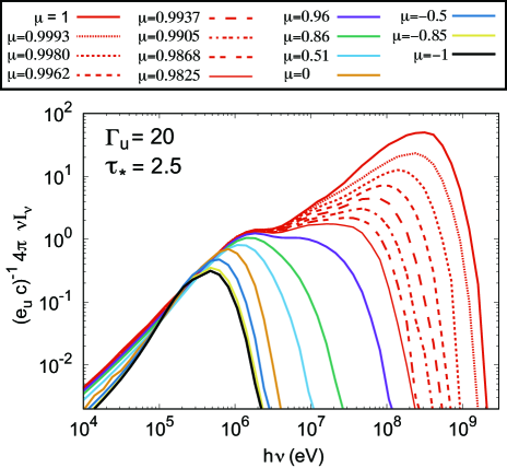
Figure 5: Shock-frame, local SEDs ($c^{-1}4\pi\nu I_{\nu}$) at the downstream location $\tau_{*}=2.5$, for $\Gamma_{\rm u}=20$. The normalization is the same as in Fig. 4. Each line shows the case for a given cosine of the angle between the direction of photon propagation and the flow velocity, $\mu=\cos\theta$. The sequence of red lines demonstrates the strong angle dependence of the beamed high energy component within a narrow range $\theta\lesssim 4/\Gamma_{\rm u}\sim 11^{\circ}$. The magenta ($\theta=16^{\circ}$), green ($\theta=30^{\circ}$), cyan ($\theta=60^{\circ}$), brown ($\theta=91^{\circ}$), blue ($\theta=120^{\circ}$), yellow ($\theta=149^{\circ}$) and black lines ($\theta=180^{\circ}$) show the dependence well outside the beaming cone.

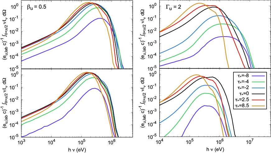
Figure 6: Shock frame, local SEDs, normalized as in Fig 4, for $\beta_{\rm u}=0.5$ (left) and $\Gamma_{\rm u}=2$ (right). The top and bottom panels show the photons propagating in an angle contained within a half hemisphere along ($\theta\leq\pi/2$) and against ($\theta>\pi/2$) the flow, respectively. Different lines correspond to the different locations at which the SEDs are evaluated, as indicated. The magenta, green, blue, black, red and yellow correponds to $\tau_{*}=-8$, $-4$, $-2$, $0$, $2.5$ and $8.5$, respectively.

3.3 Comparison with previous works

As a check on our results, we compared the shock structure obtained in the simulations with analytical and numerical solutions reported in the literature. In the upper panel of Fig. 7 we show a comparison of the Lorentz factor profiles obtained in our simulations for $\Gamma_{\rm u}=6,10$ and $20$ with those computed numerically by Budnik et al. (2010). As seen, broad agreement is found in all cases. It should be noted, however, that our simulations systematically find somewhat steeper profile (faster deceleration). One possible reason for this discrepancy might be the optimaization of the cross sections in their numerical analysis (see Appendix E for details). We stress that our code employs the full Klein-Nishina cross sections for Compton scattering and pair production, thus likely producing more accurate results. Moreover, the current simulations have advantage in that we cover a larger computational domain to avoid any effects related to boundary conditions. We also find that the flexibility of the Monte-Carlo method enables us to resolve the momentum distribution of photons with a higher precision since we inject sufficiently large number of particles to minimize statistical errors.

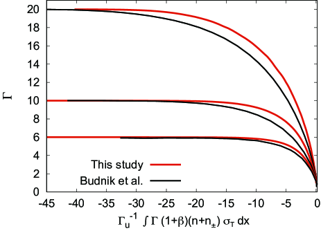
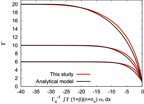
Figure 7: Comparison of the Lorentz factor profiles obtained din the simulation for $\Gamma_{\rm u}=6$, $10$ and $20$ with the numerical results of Budnik et al. (2010) (upper panel) and the analytical solutions of GNL18 (bottom panel). The profiles are given here as functions of the dimensionless variable $\Gamma_{\rm u}^{-1}\int\Gamma(1+\beta)(n+n_{\pm})\sigma_{T}dx$ used in Budnik et al. (2010), which different from the pair loaded Thomson depth $\tau_{*}$ used in Figs 1 and 2.

Next, let us consider the comparison with the analytical solution derived in GNL18. There are two free parameters in this model ($\eta$ and $a$) that reflect uncertainties associated with the distribution of photons within the shock and the fine details of energy deposition. We find that good fits can be obtained both to Budnik et al. (2010) results and to our results (see lower panel in Fig. 7) for the range of parameters $\eta=0.45-0.55$ and $a=1.5-2.5$, despite the differences mentioned above. This suggests that these differences are not due to a drastic change in the properties of shock.

Analytical solutions have also been derived for sufficiently subrelativistic infinite shocks (Blandford & Payne, 1981b), as well as finite shocks with escape (Ioka, Levinson & Nakar, 2019), by employing the diffusion approximation (e.g., Blandford & Payne, 1981a). In Appendix C (Fig. 8) we compare the shock profile obtained in the simulation for $\beta_{\rm u}=0.1$ with the analytic solution of Blandford & Payne (1981b) and find remarkable agreement, confirming the validity of the diffusion approximation up to at least $\beta_{\rm u}=0.1$.

Finally, the spectra computed in our simulations for shocks with $\Gamma_{\rm u}\geq 6$ are generally consistent with those obtained by Budnik et al. (2010), although there are some small differences in the spectral evolution just behind the shock. In particular, the emergence of the thermal bump seen in Fig. 4 by comparing the spectra at $\tau_{*}=0$ and $\tau_{*}=2.5$, which results from up-scattering of soft photons by the thermal pairs, appears to be faster in our simulations. This difference is most likely due to the larger strength of the subshock in our simulations, that gives rise to a higher temperature behind the subshock. At any rate, this difference does not affect the spectrum of the breakout signal (which is emitted in forward direction) in most situations.

4 Applications to shock breakout emission

The first signal observed during a shock breakout episode is emitted from a layer of optical thickness $\sim 1/\beta_{\rm d}$ (roughly one diffusion length) behind the shock (Weaver, 1976; Katz, Budnik, & Waxman, 2010; Nakar & Sari, 2010, 2012; Levinson & Nakar, 2019). In sudden breakouts of fast Newtonian RMS from a sharp density gradient (e.g., from a stellar envelope or the fast tail of merger ejecta), the spectrum of the breakout emission should closely resemble the spectrum computed in our simulations of infinite RMS. Our results indicate that the observed temperature in such breakouts should largely exceeds the black body limit (by up to several orders of magnitudes), and that the spectrum below the peak is very soft ($F_{\nu}\propto\nu^{0}$ roughly), with a prominent bump near the peak (see Figs. 4 and 6). GRB 060218, discussed below, may be an example. In relativistic breakouts, in which the opacity is dominated by pairs, the breakout emission is released only after the plasma cools to a temperature at which the pairs disappear (Nakar & Sari, 2012). From our results we estimate a comoving temperature of about $35$ keV at breakout, and an observed temperature of $35\Gamma_{\rm u}$ keV. Also in this case the spectrum below the peak should be very soft.

In case of shock breakout from a stellar wind the shock structure and spectrum are expected to evolve during the breakout episode due to radiative losses (GNL18, Ioka, Levinson & Nakar 2019), and further analysis is needed to make firm predictions. Such an analysis is underway.

In the following we consider some specific systems:

4.1 GRB 060218

GRB 060218 is one of the six low luminosity GRBs identified thus far (Campana et al., 2006; Soderberg et al., 2006). It is associated with SN 2006aj - a rare type double peak SN. It has long been proposed (Kulkarni et al., 1998) that, unlike regular LGRBs, llGRBs may result from a breakout of a shock driven by a choked jet, and this model has been applied to explain the properties of GRB 060218 (Campana et al., 2006; Waxman et al., 2007; Li, 2007; Nakar, 2015). It has been argued (Nakar, 2015) that the association of LGRBs and llGRBs with the same rare SN type (broad line IC), suggests that both GRB classes share the same explosion physics, but in different environments. Specifically, Nakar (2015) proposed that the key difference between llGRBs and LGRBs is the outer structure of the progenitor; while in llGRBs the compact core of the progenitor is ensheathed by an extended ($>100R_{\odot}$), low mass ($\sim 10^{-2}M_{\odot}$) envelope that chokes the jet, in LGRBs this envelope is absent. The double-peak light curve of SN 2006aj is naturally explained in this model; the first peak is associated with the cooling emission of the low mass extended envelope and the second peak is powered by radioactive decay of ⁵⁶Ni. Furthermore, the envelope parameters needed to account for the optical/UV emission of SN 2006aj around the first peak are in remarkable agreement with those needed, independently, to explain the breakout gamma-ray emission.

The shock breakout scenario for GRB 060218 has been criticized recently (Emery et al., 2019) on the grounds that it cannot account for the UV/optical spectra observed in the first $1350$ s (roughly the breakout duration in the shock breakout model), that appear to be much softer than a Rayleigh-Jeans power-law (consistent with flat spectrum, $F_{\nu}\propto\nu^{0}$, within the errors). Moreover, by the time of $\sim 2000$ s the spectrum evolved into a Rayleigh-Jeans spectrum. Emery et al. (2019) therefore proposed that the early ($<1300$ s) UV/optical emission is produced by synchrotron emission in an external shock driven by a successful, low power jet, that also produce the GRB emission. However, this appears inconsistent with the requirement that the jet penetrates all the way through the extended envelope that is needed to account for the early cooling emission of SN 2006aj, unless an engine life time in excess of 10,000 s is invoked.

Here we argue that the observed UV/optical spectrum at $t<1000$ s is in fact consistent with the shock breakout model. Our results indicate that the observed peak energy of the GRB ($\sim$ 40 keV, Kaneko et al. 2007) can be accommodated by a shock velocity of $\beta_{\rm u}\sim 0.3-0.4$ (depending somewhat on shock geometry and other details). This velocity, in turn, yields breakout energy and duration that are consistent with the observed GRB isotropic equivalent energy and duration (Nakar, 2015). From our simulations we find that for a shock velocity in this range the portion of the spectrum below the peak is roughly flat, down to a few eV, consistent with the UV/optical slope reported by Emery et al. (2019). The luminosity in the V band is lower by a factor of $\sim 10^{4}$ than the GRB luminosity at $650$ s, consistent with a roughly flat spectrum up to the X-ray band, as predicted by the RMS simulations. The evolution to the Rayleigh-Jeans regime at $t>1600$ s is also naturally expected, since the emission at these times originate form deep layers behind the shock, in which the black body limit has established.

4.2 GRB170817A

The shock breakout model for NS mergers (Kasliwal et al., 2017; Gottlieb et al., 2018; Pozanenko et al., 2018; Beloborodov et al., 2018) asserts that the gamma-ray flash observed in GRB 170817A was produced during the emergence of the shock driven by the jet-cocoon system from the fast tail leading the merger ejecta. The original model proposed by Kasliwal et al. (2017) and Gottlieb et al. (2018) has been criticized by Beloborodov et al. (2018) on the grounds that it predicts a too high SED peak for the ejecta Lorentz factor needed to accommodate observational constraints. Here we point out that, contrary to this claim, the sensitive dependence of the temperature on shock velocity allows sufficient freedom to consistently account for all observables. As shown recently (Nakar, 2019), the model can reproduce the burst energy and duration, given the observed delay between the NS collision and the onset of the burst, for shock velocities in the range $0.25\lesssim\beta_{\rm u}\lesssim 0.6$. According to our simulations, this corresponds to the range of comoving temperature at breakout of 10 keV $\lesssim kT\lesssim 35$ keV (the upper limit is the temperature at which pairs disappear). With an ejecta Lorentz factor of $\Gamma=5$ invoked in Beloborodov et al. (2018) this gives a peak energy in the range $200-500$ keV, consistent with the observations. We stress that our estimate assumes H-rich composition. Heavy composition, particularly r-process, would imply a lower temperature, but still in a range consistent with the observations (Nakar, 2019).

5 Summary and conclusions

We performed Monte-Carlo simulations of photon-starved RMS over a broad range of shock 4-velocities. In these shocks, the (cold) upstream flow decelerates via bulk Comptonization of counterstreaming photons that are generated inside and just behind the shock by bremsstrahlung emission. Six models, that cover the fast Newtonian ($\beta_{\rm u}=0.1$), trans-relativistic ($\beta_{\rm u}=0.5$), mildly relativistic ($\Gamma_{\rm u}=2$) and fully relativistic ($\Gamma_{\rm u}=6,10$ and $20$) regimes are thoroughly investigated. All models invoke a pure H composition at a fiducial density of $n_{\rm u}=10^{15}$ cm^-3 in the far upstream flow. This is the first time that self-consistent calculations of the shock structure and spectrum in the fast Newtonian and mildly relativistic regimes ($\Gamma_{\rm u}<6$) are performed. Our results for fully relativistic ($\Gamma_{\rm u}\geq 6$) RMS are in good agreement with the numerical solutions obtained by Budnik et al. (2010), and the analytical solutions derived by Nakar & Sari (2012) and Granot, Nakar & Levinson (2018) for the shock profile. The main findings are:

(i) Our simulations confirm that in the fast Newtonian regime ($0.05\lesssim\beta_{\rm u}\lesssim 0.5$) the immediate downstream temperature depends sensitively on shock velocity (roughly as $\beta_{\rm u}^{3}$), whereas in relativistic shocks it is regulated by exponential pair creation, and lies in the range $100-200$ keV, with a very weak dependence on $\Gamma_{\rm u}$. For the assumed density and composition (pure H), the transition to pair dominance was found to occur at $\beta_{\rm u}=0.5$, as anticipated earlier. For r-process composition it is expected to occur at somewhat higher velocity (Levinson & Nakar, 2019). In Section 4 we discussed the implications of the sensitive dependence of $T$ on $\beta_{\rm u}$ for the shock breakout model of GRB 170817A.

(ii) In all cases explored ($\beta_{\rm u}\geq 0.1$) the radiation in the immediate downstream is out of thermodynamic equilibrium due to insufficient photon generation. The black body limit is reached only relatively far downstream. As a result, the spectrum below the $\nu F_{\nu}$ peak is considerably softer than the Planck spectrum down to a break frequency that depends on shock velocity, below which the spectrum hardens ($F_{\nu}\propto\nu^{2}$). This implies a much brighter optical emission in fast Newtonian and relativistic breakouts than naively estimated by invoking Wien spectrum below the peak, with important consequences for the detection rate of shock breakout candidates. In particular, we argued that the softening of the spectrum below the peak is consistent with the early X/UV/optical emission detected in GRB 060218. A detailed analysis of the observational consequences is underway.

(iii) In relativistic shocks the photon distribution inside the shock is highly anisotropic. For the photon beam that subtends an angle $\sim 1/\Gamma_{\rm u}$ around the flow direction (that is, moving towards the downstream), the spectrum above the peak extends to an energy of $\Gamma_{\rm u}^{2}m_{e}c^{2}$ in the shock frame. This should not affect the observed spectrum in most relativistic breakouts, but might have some effect on the high energy spectrum in mildly relativistic, aspherical breakouts, which are expected in cases where the shock is driven by a jet as, e.g., in BNS mergers and llGRB. The reason is that an observer located at some angle to the axis will receive contributions from different parts of the shock, each moving at a different Lorentz factor and in a different direction.

(iv) While in fast and mildly relativistic RMS the shock transition is smooth, relativistic RMS ($\Gamma_{\rm u}\geq 2$) exhibit subshocks with a local velocity jump of $\delta(\Gamma\beta)\sim 0.2-0.7$ for $\Gamma_{\rm u}=2-20$, and a non-negligible strength. We find that a few percents of the total shock energy dissipate in the subshock. It is unclear at present wether these subshocks can accelerate particles to highly relativistic energies, but if they can it might significantly affect the emitted spectrum. Further investigation is needed to quantify the effect of the subshock on the high energy emission.

Our simulations provide an important insight into the properties of fast and relativistic RMS, and their role in shaping the shock breakout signal in energetic supernovae, low luminosity GRBs and NS mergers. The results of our simulations can be employed to predict the spectral evolution during the breakout phase under conditions anticipated in specific systems. However, the present analysis applies to infinite shocks and may not be adequate enough to describe breakouts from stellar winds, in which radiative losses become gradually important during the breakout phase, changing the shock structure (GNL18, Ioka, Levinson & Nakar 2019). Our Monte-Carlo technique has been generalized recently to finite RMS with radiative losses, and the investigation of such shocks is currently in progress, and will be reported in a future publication (Ito, Levinson & Nakar, in preparation).

Appendix A IMPLEMENTING BREMSSTRAHLUNG EMISSION AND ABSORPTION

The Monte-Carlo code used in this study handles transfer of photons in a medium at which Compton scattering, pair creation/annihilation, and bremsstrahlung emission/absorption take place. The description of the original code that includes the former two processes is given in Paper I. Here we outline the implementation of the bremsstrahlung process in the modified code. Following the notations in Paper I, we label quantities that are measured in the comoving frame of the bulk plasma with the superscript prime symbol.

A.1 Bremsstrahlung emission

The modified code includes photon production by $e^{\pm}p$, $e^{-}e^{+}$, $e^{-}e^{-}$ and $e^{+}e^{+}$ thermal bremsstrahlung. The photon generation rate in the fluid rest frame is given by (Svensson, 1982)

$$\left(\frac{dN_{\gamma}}{dt^{{}^{\prime}}d\nu^{{}^{\prime}}d\Omega^{{}^{\prime}}dV^{{}^{\prime}}}\right)_{\rm ff}=\sqrt{\frac{1}{6\pi^{3}}}~{}\alpha_{f}\sigma_{T}cn^{2}\frac{1}{\nu^{{}^{\prime}}\sqrt{\Theta}}~{}{\rm exp}\left(-\frac{h\nu^{{}^{\prime}}}{kT}\right)\lambda_{\rm ff},$$ (2)

where $\Theta=kT/m_{e}c^{2}$ denotes the plasma temperature in units of the electron mass, and $\alpha_{f}$ is the fine structure constant. Here $n$ denotes the baryon density, and

$$\lambda_{\rm ff}=(1+2x_{+})g_{ep}+[x_{+}^{2}+(1+x_{+})^{2}]g_{ee}+x_{+}(1+x_{+})g_{\pm}$$ (3)

is a dimensionless factor that depends on the pair-to-baryon density ratio, $x_{+}=n_{\pm}/2n$, and the Gaunt factors $g_{ep}$, $g_{ee}$ and $g_{\pm}$ that correspond to $e^{\pm}p$, $e^{\pm}e^{\pm}$ and $e^{-}e^{+}$ encounters, respectively. As for the Gaunt factors, we employ the analytic fits given in Skibo et al. (1995) which are expressed as functions of temperature and frequency. Note that there is an errata for this paper (Skibo et al., 1996).

The photon generation rate in the shock frame is related to the rate in the fluid frame through

$$\left(\frac{dN_{\gamma}}{dtd\nu d\Omega dV}\right)_{\rm ff}={\cal D}\left(\frac{dN_{\gamma}}{dt^{{}^{\prime}}d\nu^{{}^{\prime}}d\Omega^{{}^{\prime}}dV^{{}^{\prime}}}\right)_{\rm ff},$$ (4)

where ${\cal D}=[\Gamma(1-\beta{\rm cos}\theta)]$ is the Doppler factor. In our code, photon packets are injected at every grid point in the numerical domain with a probability proportional to the local photon generation rate. We employ a fixed value for the photon number per packet, $n_{\gamma,{\rm pack}}$, in all grid points, and the injecting rate of the packet number per unit volume for a given range of solid angles $d\Omega$ and frequencies $d\nu$ is given by $\int\int\left(\frac{dN_{\gamma}}{dtd\nu d\Omega dV}\right)_{\rm ff}(n_{\gamma,{pack}})^{-1}d\Omega d\nu$.

Since the photon generation rate scales as $\left(\frac{dN_{\gamma}}{dtd\nu d\Omega dV}\right)_{\rm ff}\propto\nu^{-1}$ in the low frequency limit ($\nu\ll kT$), the produced number of photons diverges logarithmically at low energy. Therefore, we must impose a lower limit on the frequency that we take into accout in order to avoid divergence. Here, we follow the prescription employed in Budnik et al. (2010) for the minimum frequency which is determined from

$$\nu_{min}=\frac{\gamma_{e,th}^{2}\beta_{e,th}c}{2\pi\lambda_{D}},$$ (5)

where $\lambda_{D}=\sqrt{kT/4\pi e^{2}(n+0.5n_{\pm})}$ is the Debye length and $\gamma_{e,th}=1+3/2f(T)\Theta$ and $\beta_{e,th}=\sqrt{1-\gamma_{e,th}^{-2}}$ are the Lorentz factor and velocity of the theral motion of electrons, respectively. Here $f(T)={\rm tanh}[({\rm ln}\Theta+0.3)/1.93]+3/2$ is an analytical function of temperature defined in Budnik et al. (2010), obtained from a fit to the exact equation of state of pairs. Photons at low frequency is produced at impact factor larger than the Debye length, and therefore the bremsstrahlung emission is suppressed due to Coulomb screening.

A.2 Bremsstrahlung absorption

The opacity for the bremsstrahlung process is determined from the Kirchhoff’s law for radiation. In terms of the photon generation rate it is give by

$$\alpha^{{}^{\prime}}(\nu^{{}^{\prime}},T)=\left(\frac{dN_{\gamma}}{dt^{{}^{\prime}}d\nu^{{}^{\prime}}d\Omega^{{}^{\prime}}dV^{{}^{\prime}}}\right)_{\rm ff}\frac{h\nu^{{}^{\prime}}}{B_{\nu}(\nu^{{}^{\prime}},T)}$$ (6)

in the fluid rest frame, where $T(x)$ is the local temperature, and $B_{\nu}(\nu,T)=2h\nu^{3}/c^{2}[{\rm exp}(h\nu/kT)-1]^{-1}$ is the corresponding Planck function. With the known opacity, the distance a photon packet propagates before being absorbed is determined in the same manner as in the case of Compton scattering and photon-photon pair creation (see paper I). In brief, we randomly draw a value for the optical depth, say $\delta\tau$, and then determine the physical distance $l$ in the laboratory frame, using the implicit equation $\delta\tau=\int^{l}_{0}{\cal D}\alpha^{{}^{\prime}}dx$.

Appendix B BOUNDARY CONDITIONS

As for the boundary conditions at far upstream, we employ the same method used in Paper I. We inject photons with photon-to-baryon number ratio given by $\tilde{n}_{\rm u}=n_{\gamma{\rm u}}/n_{\rm u}=10$ at the boundary. The energy contained in the injected photons is negligible compared to the baryons ($\tilde{n}_{\rm u}kT_{\rm u}/m_{p}c^{2}\ll 1$). The injected spectrum is Wien, characterized by the local temperature in the comoving frame. The temperature at the boundary is set as $T_{\rm u}=(3kn_{\gamma{\rm u}}/a_{rad})^{1/3}$ under the assumption it is close to the blackbody limit, where $a_{rad}$ is the radiation density constant. Note that, while the assumption of blackbody contradicts with the assumption of Wien spectrum, the spectral feature is only noticable at far upstream region and is quickly smeared out by the emission/absoption process. It is emphasized that the current boundary condition is adopted for numerical convenience, and has no noticeable effect on the results, since the injected (advected) photon population is highly sub-dominant compared to the photons that are generated inside the shock.

We also inject photons at the far downstream boundary in order to maintain the radiation field there isotropic in the comoving frame, with a Wien spectrum which is determined by the local plasma temperature. The normalization of the photon’s energy distribution is iteratively adjusted to match the outgoing photos flux at the boundary. It is noted that, while the assumption that the radiation is isotropic can be justified, the choice of a Wien spectrum at the boundary is approximate, since in practice the spectrum tends to approach the Planck distribution. Nonetheless, this should not affect the results drastically since the downstream boundary is located at a distance from the shock which is larger than the diffusion length, so that photons injected at the downstream boundary cannot reach the shock and, therefore, cannot affect its dynamics.

To sum up, as in Paper I, the photon flux at the upstream and downstream boundaries in the laboratory frame is a function of the photon number density and temperature, and can be written as

$$\frac{dN_{\gamma}}{dtd\nu d\Omega dS}={\cal D}^{2}\frac{dN_{\gamma}}{dt^{{}^{\prime}}d\nu^{{}^{\prime}}d\Omega^{{}^{\prime}}dS^{{}^{\prime}}},$$ (7)

where

$$\frac{dN_{\gamma}}{dt^{{}^{\prime}}d\nu^{{}^{\prime}}d\Omega^{{}^{\prime}}dS^{{}^{\prime}}}=\frac{n_{\gamma}}{8\pi}\left(\frac{h}{kT}\right)^{3}\nu^{{}^{\prime}2}{\rm exp}\left(-\frac{h\nu^{{}^{\prime}}}{kT}\right).$$ (8)

Thus, for a given range of solid angles $d\Omega$ and frequencies $d\nu$, $\frac{dN_{\gamma}}{dtd\nu d\Omega dS}(n_{\gamma,{pack}})^{-1}{\rm cos}\theta d\Omega d\nu$ gives the injection rate of the packet number per unit area of the boundary surface, where $n_{\gamma,{\rm pack}}$ is the number of photons contained in a single packet. However, it is again emphasized that the boundary conditions do not effect the solutions, which is governed by the photons that are generated inside the shock and within one diffusion length behind it.

Appendix C COMPARISON WITH ANALYTIC SOLUTION IN NON-RELATIVISTIC REGIME

Here we compare our simulation for $\beta_{\rm u}=0.1$ with the analytic solution of a diffusive shock. When the speed of the upstream flow is well below the speed of light, $\beta_{\rm u}\ll 1$, diffusion approximation can be applied to solve the RMS structure. This approximation yields an universal velocity profile which depends only on an optical depth defined as ${d\hat{\tau}}=\beta_{\rm u}\int n\sigma_{T}dx$ (see e.g., Blandford & Payne, 1981b; Katz, Budnik, & Waxman, 2010; Ioka, Levinson & Nakar, 2019):

$$\frac{\beta}{\beta_{\rm u}}=\frac{4}{7}+\frac{3}{7}{\rm tanh}\left[-\frac{3}{2}\hat{\tau}\right].$$ (9)

Here $\hat{\tau}=0$ is located roughly at the center of the shock $\beta/\beta_{\rm u}=4/7$, and $\hat{\tau}\rightarrow-\infty$ ($\hat{\tau}\rightarrow+\infty$) and correspond to the far upstream (far downstream). The red crosses in Fig. 8 delineate the result of our simulation and the black solid line the analytic solution. As is seen the agreement is remarkable. The fact that our code is capable of reproducing the universal profile to such an accuracy reassures that our calculations are highly reliable.

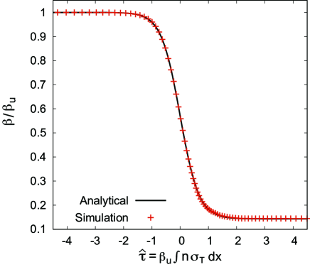
Figure 8: Comparison of the velocity structure obtained in our simulation for $\beta_{\rm u}=0.1$ (red crosses) and the analytical solution Eq. (9) (black solid line).

Appendix D SED EVOLUTION FOR $\beta_{\rm u}=0.1$

Here we examine the evolution of the SED at the downstream region for $\beta_{\rm u}=0.1$. We remark that while the velocity structure shows universal profile as described in Appendix C, The temperature and, consequently, the spectrum depend on the composition and density $n_{\rm u}$ far upstream. In this section, we consider a pure H composition at a density $n_{\rm u}=10^{15}~{}{\rm cm}^{-3}$.

As stated in the main text, under these conditions the radiation in the immediate downstream, in the $\beta_{\rm u}=0.1$case, is marginally out of thermodynamic equilibrium. Our simulation yields a plasma temperature of $kT\sim 520~{}{\rm eV}$ at the end of the deceleration zone ($\tau_{*}=0$), which is factor of a few higher than the black body limit ($kT_{\rm d}\simeq 130~{}{\rm eV}$). At the downstream region, thermalization proceeds owing to continuous photon generation by the bremsstrahlung emission. As a result, the plasma cools and the spectrum evolves towards a Planckian. For illustration, we plot in Fig. 9 the spectrum (red line) at two different downstream locations, just behind the shock ($\tau_{*}=2.5$) and at one diffusion length away ($\tau_{*}=67$). A slow evolution into a Planck spectrum (shown as the black line) is evident, and it is clear that a full thermodynamic equilibrium will be established only at a few diffusion lengths downstream. The important implication is that the spectrum of the breakout emission should be much softer than Planck.

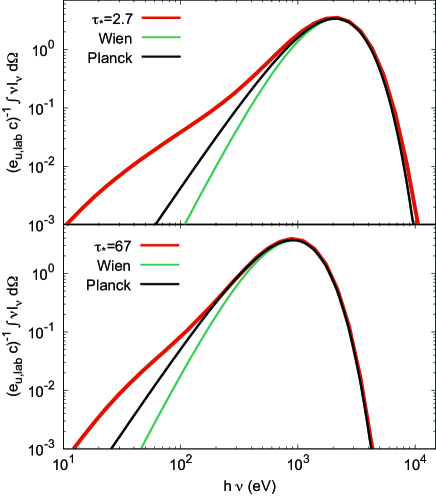
Figure 9: Comparison of the local SEDs in the downstream region normalized by the energy density of the far upstream $e_{\rm u}=\Gamma_{\rm u}(\Gamma_{\rm u}-1)n_{\rm u}m_{p}c^{2}$ for the model with velocity of $\beta_{\rm u}=0.1$ (red) with the Planck (black) and Wien distribution (green). Note that the anisotropy of photons is negligible in this case. The top and bottom panels correspond to the locations $\tau_{*}=2.7$ and $\tau_{*}=67$, respectively. In the top (bottom) panel, the temperature of the Planck and Wien distributions is $kT=530~{}{\rm eV}$ ($kT=230~{}{\rm eV}$).

Appendix E DIFFERENCE FROM Budnik et al. (2010)

In this appendix we compare some technical aspects between our simulation method and that of Budnik et al. (2010), in an attempt to elucidate the origin of the differences between the results of the two simulations indicated in the main text.

The two codes incorporate exactly the same radiation interactions (Compton scattering, pair production/annihilation and bremsstrahlung emission/absorption). However, while our method use the exact cross sections for all reactions, Budnik et al. (2010) use some approximations to compute Compton scattering. First, they assume that the scattering is isotropic in the fluid rest frame, which is inaccurate in the Klein-Nishima regime. Second, they use an approximate form for the comoving energy redistribution function of scattered photons, that keeps a relativistic Wien distribution invariant under scattering. As shown below, this form is not precise since it is not based on the exact cross section. The cumulative effect of their approximations is an overestimate of the mean energy deposition inside and upstream of the shock. While we cannot completely rule out other causes, we tend to believe that this overestimate is the reason for the quantitative difference in temperature and velocity profiles.

A comparison of the redistribution function adopted in Budnik et al. (2010) and the exact one computed in our simulation by using the full cross section is exhibited in Fig. 10. Here the incident comoving photon energy and the plasma temperature are taken to be $h\nu_{\rm in}=40m_{e}c^{2}$ and $kT=6m_{e}c^{2}$, respectively, which are typical values for the backstreaming photons and the plasma temperature at the deceleration zone in the $\Gamma_{\rm u}=20$ simulation; the difference is clear. In particular, the mean energy of scattered photons is larger in our simulations. This discrepancy is qualitatively similar for other incident energies and plasma temperatures. Consequently, the calculations of Budnik et al. (2010) tend to systematically underestimate the population of high energy photons, implying that the energy gain of the plasma (heating) per scattering is overestimated in their simulation.

In Fig. 11 we plot the ratio between the values of the average energy deposition per scattering obtained in our simulation and in those of Budnik et al. (2010). As seen, for $h\nu_{\rm in}>3kT$ the average energy deposition per scattering computed in Budnik et al. (2010) is larger by $\sim 20-30{\%}$. While these systematic errors are modest, they accumulate in a nonlinear manner that can somewhat alter the shock profile.

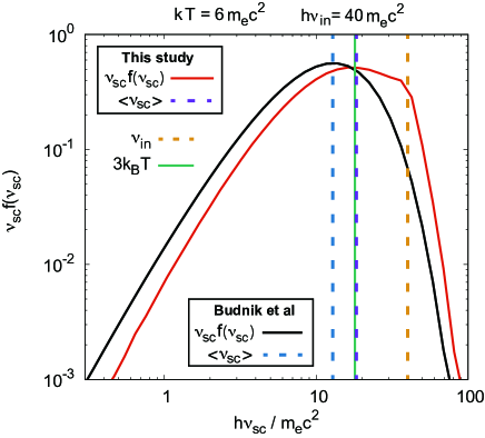
Figure 10: Energy redistribution function of scattered photons for incident photon energy of $h\nu_{\rm in}=40m_{e}c^{2}$, injected in a thermal pool of electrons having a temperature $kT=6m_{e}c^{2}$. Here the redistribution function $f(\nu_{\rm sc})d\nu_{\rm sc}$ gives the probability for the scattered photon energy to be in the range $[\nu_{\rm sc}:\nu_{\rm sc}+d\nu_{\rm sc}]$. The red solid line shows the exact function obtained from our calculations, while the black line shows the analytic function employed in Budnik et al. (2010). The dashed lines represent the incident photon energy (brown), and the average scattered photon energy obtained in our simulations (magenta) and in Budnik et al. (2010) (blue). The green solid line marks the typical energy of electrons, $3kT$, and is shown for reference.

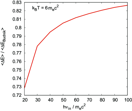
Figure 11: Ratio between the exact value of the mean energy deposition per scattering obtained in our simulations, $<\Delta E>$, and the value computed in Budnik et al. (2010), $<\Delta E_{\rm Budnik}>$. The average $<\Delta E>$ is taken over the distribution of incident photons $f(\nu_{\rm in}$), each deposit a mean amount $\Delta E=h(\nu_{\rm in}-<\nu_{\rm sc}>)$ in a single scattering.

References

- Beloborodov (2017) Beloborodov A. M., 2017, ApJ, 838, 125
- Beloborodov et al. (2018) Beloborodov, A. M., Lundman, C., & Levin, Y. 2018, arXiv e-prints, arXiv:1812.11247
- Blandford & Payne (1981a) Blandford R. D., Payne D. G., 1981a, MNRAS, 194, 1033
- Blandford & Payne (1981b) Blandford R. D., Payne D. G., 1981b, MNRAS, 194, 1041
- Bromberg et al. (2011) Bromberg O., Mikolitzky Z., Levinson A., 2011, ApJ, 733, 85
- Budnik et al. (2010) Budnik R., Katz B., Sagiv A., Waxman E., 2010, ApJ, 725, 63
- Beloborodov et al. (2018) Beloborodov, A. M., Lundman, C., & Levin, Y. 2018, arXiv e-prints, arXiv:1812.11247
- Campana et al. (2006) Campana, S., Mangano, V., Blustin, A. J., et al. 2006, Nature, 442, 1008
- Emery et al. (2019) Emery, S. W. K., Page, M. J., Breeveld, A. A., et al. 2019, MNRAS, 484, 5484
- Gottlieb et al. (2018) Gottlieb, O., Nakar, E., Piran, T., & Hotokezaka, K. 2018, MNRAS, 479, 588
- Granot, Nakar & Levinson (2018) Granot A., Nakar E., Levinson A., 2018, MNRAS, 476, 5453 (GNL18)
- Ioka, Levinson & Nakar (2019) Ioka K., Levinson A., Nakar E., 2019, MNRAS, 484, 3502
- Ito et al. (2018) Ito H., Levinson A., Stern B. E., Nagataki S., 2018, MNRAS, 474, 2828 (Paper I)
- Katz, Budnik, & Waxman (2010) Katz B., Budnik R., Waxman E., 2010, ApJ, 716, 781
- Kulkarni et al. (1998) Kulkarni, S. R., Frail, D. A., Wieringa, M. H., et al. 1998, Nature, 395, 663
- Kaneko et al. (2007) Kaneko, Y., Ramirez-Ruiz, E., Granot, J., et al. 2007, ApJ, 654, 385
- Kasliwal et al. (2017) Kasliwal, M. M., Nakar, E., Singer, L. P., & et. al. 2017, Science, 358, 1559
- Keren & Levinson (2014) Keren S., Levinson A., 2014, ApJ, 789, 128
- Levinson (2012) Levinson A., 2012, ApJ, 756, 174
- Levinson & Bromberg (2008) Levinson A., Bromberg O., 2008, Phys. Rev. Lett., 100, 131101
- Levinson & Nakar (2019) Levinson A., Nakar E., 2019, arXiv, arXiv:1909.10288
- Li (2007) Li, L.-X. 2007, MNRAS, 375, 240
- Lundman, Beloborodov & Vurm (2018) Lundman C., Beloborodov A. M., Vurm I., 2018, ApJ, 858, 7
- Lyubarskij & Sunyaev (1982) Lyubarsky Y. E., Sunyaev R. A., 1982, Soviet Astron. Lett, 8, 330
- Nakar & Sari (2010) Nakar E., Sari R., 2010, ApJ, 725, 904
- Nakar & Sari (2012) Nakar E., Sari R., 2012, ApJ, 747, 88
- Nakar (2015) Nakar, E. 2015, ApJ, 807, 172
- Nakar (2019) Nakar E., 2019, to be submitted to PR
- Pai (1966) Pai S. I., 1966, Radiation Gas Dynamics, Springer, New York
- Pozanenko et al. (2018) Pozanenko, A. S., Barkov, M. V., Minaev, P. Y., et al. 2018, ApJL, 852, L30
- Riffert (1988) Riffert H., 1988, ApJ, 327, 760
- Skibo et al. (1995) Skibo J. G., Dermer C. D., Ramaty R., McKinley J. M., 1995, ApJ, 446, 86
- Skibo et al. (1996) Skibo J. G., Dermer C. D., Ramaty R., McKinley J. M., 1996, ApJ, 463, 391
- Soderberg et al. (2006) Soderberg, A. M., Kulkarni, S. R., Nakar, E., et al. 2006, Nature, 442, 1014
- Svensson (1982) Svensson R., 1982, ApJ, 258, 335
- Waxman et al. (2007) Waxman, E., Mészáros, P., & Campana, S. 2007, ApJ, 667, 351
- Weaver (1976) Weaver T. A., 1976, ApJS, 32, 233
- Zel’dovich & Raizer (1967) Zel’dovich Y. B., Raizer Y. P., 1967, Physics of shock waves and high-temperature hydrodynamic phenomena