Observation of quantum many-body effects due to zero point fluctuations in superconducting circuits

Electromagnetic fields possess zero point fluctuations (ZPF) which lead to observable effects such as the Lamb shift and the Casimir effect. In the traditional quantum optics domain, these corrections remain perturbative due to the smallness of the fine structure constant. To provide a direct observation of non-perturbative effects driven by ZPF in an open quantum system we wire a highly non-linear Josephson junction to a high impedance transmission line, allowing large phase fluctuations across the junction. Consequently, the resonance of the former acquires a relative frequency shift that is orders of magnitude larger than for natural atoms. Detailed modelling confirms that this renormalization is non-linear and quantum. Remarkably, the junction transfers its non-linearity to about 30 environmental modes, a striking back-action effect that transcends the standard Caldeira-Leggett paradigm. This work opens many exciting prospects for longstanding quests such as the tailoring of many-body Hamiltonians in the strongly non-linear regime, the observation of Bloch oscillations, or the development of high-impedance qubits.

Introduction

The realization of many-body effects in quantum matter, often associated with remarkable physical properties, hinges on strong interactions between constituents. Mechanisms to achieve strong interactions include the Coulomb interaction in narrow band electronic materials, and Feshbach resonances that can produce arbitrarily large scattering lengths in ultra-cold atomic gases. In contrast, while providing great design versatility, purely photonic platforms, Greentree et al. (2006); Carusotto and Ciuti (2013); Le Hur et al. (2016) are not easily amenable to realizing strong correlations, since they usually come with weak non-linearity. To circumvent this, superconducting circuits, which operate in the microwave range and display high tunability, have been proposed Houck et al. (2012) for the exploration of correlated states of light. Here, correlations originate from non-linear elements, such as Josephson junctions, and the enhancement of non-linearities is accompanied by large zero point fluctuations (ZPF). This can be understood in the electronics language of impedance as follows. The dynamics of a Josephson junction is described by two conjugate variables: the number of transferred Cooper pairs $\hat{n}$ and the superconducting phase difference $\hat{\phi}$. Despite being an anharmonic oscillator, a Josephson junction with Josephson energy $E_{\text{J}}$ and charging energy $E_{\text{c}}$, can be associated to an impedance $Z_{\text{J}}=\hbar/(2e)^{2}\sqrt{2E_{\text{c}}/E_{\text{J}}}$ which sets the amplitude of the fluctuations of $\hat{n}$ and $\hat{\phi}$. When $\big{<}\hat{\phi}^{2}\big{>}$ is sufficiently smaller than unity, $\big{<}\hat{\phi}^{2}\big{>}\propto Z_{\text{J}}/R_{\text{Q}}$ and $\big{<}\hat{n}^{2}\big{>}\propto R_{\text{Q}}/Z_{\text{J}}$, with $R_{\text{Q}}=h/(2e)^{2}\simeq$6.5\text{\,}\mathrm{k\SIUnitSymbolOhm}\text{/}$$ the superconducting quantum of resistance. Consequently, at low $Z_{\text{J}}$, phase fluctuations are weak and the anharmonic Josephson cosine potential $E_{\text{J}}(1-\cos\hat{\phi})$ can be reduced to a quadratic potential plus a quartic perturbation, as is the case for the transmon qubit Koch et al. (2007). On the other hand, if $Z_{\text{J}}$ is large, the full cosine potential is explored due to strong phase fluctuations. Anharmonicity then becomes important, as observed with the Cooper-pair box Vion et al. (2002) or the fluxonium qubit  Manucharyan et al. (2009), and as a result, the oscillation frequency $\omega_{\text{J}}$ can strongly deviate from the harmonic value $\sqrt{2E_{\text{J}}E_{\text{C}}}$. Thus, exploring many-body physics in circuit quantum electrodynamics must rely on a careful tailoring of ZPF.

The approach Weiss (1992) that we follow to explore many-body effects originating from a single non-linear superconducting element is to couple it to many harmonic modes. In the presence of such an environment, the degree of anharmonicity of a non-linear junction will also depend on the external impedance, and three regimes can be identified. When $Z_{\text{J}}$ does not match the environmental impedance $Z_{\text{env}}(\omega)$ at frequencies $\omega$ close to $\omega_{\text{J}}$, the junction is accurately described as an almost isolated system, so that the effect of the environment only amounts to small perturbative corrections, similar to the Lamb shift Fragner et al. (2008). At the same time, an impedance-mismatched environment remains weakly perturbed by the non-linear junction, and this absence of back-action allows it to be described as a set of harmonic oscillators, following the Caldeira-Leggett approach Leggett et al. (1987). This simplified description is at the core of the current understanding of open quantum systems, and was already verified experimentally in the early studies of macroscopic quantum tunneling Clarke et al. (1988). The important role of ZPF in the damping effect that such an environment has on a Josephson junction was already noticed experimentally Schwartz et al. (1985) and explained theoretically Zaikin and Panyukov (1986); Panyukov and Zaikin (1988) three decades ago. In these early works, the effect of ZPF was to renormalize junction properties such as the critical DC current by about $1\%$, which nonetheless had a large effect on macroscopic quantum tunnelling rates. When $Z_{\text{env}}\sim Z_{\text{J}}\ll R_{\text{Q}}$, the junctions and its environment fully hybridize, since they are impedance matched, but the anharmonicity of the junction remains weak and can be treated pertubatively Nigg et al. (2012); Bourassa et al. (2012); Weissl et al. (2015a); Puertas Martinez et al. (2019). The case $Z_{\text{env}}\sim Z_{\text{J}}\sim R_{\text{Q}}$ is much more challenging, both experimentally and theoretically since the strongly anharmonic junction hybridises with many modes of its environment. In DC measurements, such effects result in the celebrated Schmid-Bulgadaev transition predicted more than thirty years ago Schmid (1983); Bulgadaev (1984), a localization phenomenon whose relevance for microwave AC measurements requires further experimental and theoretical investigations Murani et al. (2019). The environment provides a strong action on the junction, which itself induces a sizeable back-action on many modes of the environment, the combined circuit forming a complex many-body system reminiscent of quantum impurity problems encountered in condensed matter Schön and Zaikin (1990). More specifically, the frequency shift induced by the environment on the junction can be comparable to $\omega_{\text{J}}$, a non-perturbative effect due to a modification of the vacuum Hekking and Glazman (1997). At the same time, the non-linearity of the junction is transferred into the environmental modes, affecting for instance their broadening, and producing a physical regime that was not addressed so far.

In this work, we report on the effects of zero point fluctuations in a device consisting of a fully characterized multi-mode environment and a highly non-linear single Josephson junction, acting as a weak link between two linear transmission lines, with all subsystems reaching the high impedance regime. As a result, the transmission of single photons through our device is strongly affected by the interplay of non-linearities and zero point fluctuations. We observe a 30% renormalization of the junction frequency as compared to the value that would have been obtained without ZPF – analogous to a giant Lamb shift – and we provide clear evidence for modifications of the environmental vacuum, which inherits strong non-linear effects. A detailed temperature analysis of our system proves the quantum origin of these fluctuations and eliminates an explanation in terms of classical hybridization effects. Finally, our experimental findings are in quantitative agreement with a microscopic theory based on the self-consistent harmonic approximation (SCHA), embedded within a fully-fledged microscopic description of our circuit using microwave simulation tools.

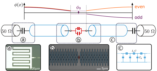
Figure 1: SQUID chains coupled to a small Josephson junction (weak link). The upper part represents the spatial phase distribution of the two first standing waves or resonant modes of the total system (Josephson junction + chains). And odd (even) mode – which couples (does not couple) to the junction – is represented in purple (orange). The lower part is a schematic of the system. The SQUID chains, depicted as blue transmission lines, are capacitively coupled to the input and output 50 Ohm coaxial cables and galvanically coupled to the small Josephson junction (in red). a Optical picture of the input and output capacitive couplings. b SEM picture of a few of the SQUIDs (1500 in total for each chain) that are coupled to the small Josephson junction (in red). c Equivalence between the transmission line effective picture and the SQUID chain characterized by three microscopic parameters $L$ and $C$ the inductance and capacitance per SQUID respectively and $C_{g}$ the ground capacitance.

Results

Background
The many-body regime of a single non-linear junction coupled to a high impedance environment has remained largely unexplored experimentally, since obtaining $Z_{\text{env}}\sim R_{\text{Q}}$ at gigahertz frequencies is very challenging. One option is to use on-chip resistors Kuzmin et al. (1991). However, this is may lead to unwanted Joule heating Huard et al. (2007). Therefore, we rather pursue a solution that relies on superconducting (lossless) high inductance materials such as Josephson junction arrays Manucharyan (2012); Masluk et al. (2012); Bell et al. (2012), noting that disordered superconductors Maleeva et al. (2018) are also promising. In Josephson junction arrays, $Z_{\text{env}}=\sqrt{L/C}$ can reach $R_{\text{Q}}$ given the large inductance of these materials, while maintaining good quality factors in the device.

Early experiments have embedded ultra-small Josephson junctions between highly resistive leads, demonstrating the incoherent tunneling of Cooper pairs Kuzmin et al. (1991) in the framework of the $P(E)$ theory Ingold and Nazarov (1992). In this case however, no supercurrent flows through the junction and no quantum coherent effects were observed. Later, the phase/charge duality in the regime $Z_{\text{J}}$, $Z_{\text{env}}$ > $R_{\text{Q}}$ was explored using SQUID arrays as the environment Corlevi et al. (2006); Ergül et al. (2013); Weissl et al. (2015b). Experimental results were explained by fluctuations due to the finite temperature of the electromagnetic environment and the effect of zero-point fluctuations could not be investigated. Moreover, these two series of experiments relied on DC measurements. This has the disadvantage that non-equilibrium effects need to be taken into account when results are interpreted, while the system is not directly probed at the finite frequencies – around $\omega_{\text{J}}$ – that are of greatest interest.

It has since become possible to obtain a frequency-resolved picture of the environment of quantum systems such as Josephson junctions, thanks to the advent of circuit QED Wallraff et al. (2004). Here, microwave techniques allow a more accurate examination of the effects of zero point fluctuations on Josephson junctions Hoi et al. (2015), and observations of perturbative spectral shifts (below 1%) attributed to ZPF were reported Fragner et al. (2008); Silveri et al. (2019); Wen et al. (2019). Several bottom-up experiments explored nonperturbative effects of light-matter interaction at ultra-strong coupling between a qubit and a single-mode resonator (for a review see Forn-Díaz et al. (2018); Kockum et al. (2019)). An effect similar to the Lamb shift – a reduction of the effective Josephson energy – was also reported recently for a DC-biased Josephson junction coupled to a single mode high impedance resonator Rolland et al. (2019). Moving towards many-body territory, a non-perturbative renormalization of the frequency of a flux qubit was demonstrated Forn-Díaz et al. (2017); Magazzù et al. (2018). However, in this experiment, fluctuations were mainly thermal, and in addition, the environment cutoff frequency could not be clearly measured. The resulting unknown parameters prevented a quantitative modeling of the experiments. Indeed, as pointed by various authors Garcia-Ripoll et al. (2015); Malekakhlagh et al. (2017); Gely et al. (2017); Parra-Rodriguez et al. (2018), it is necessary to account for all the microscopic details of the circuit to get rid of unphysical divergences in multi-mode models. Furthermore, a thorough modeling of such circuits is mandatory to discriminate the trivial effects of normal mode splitting (spectral shifts observed when two classical harmonic oscillators hybridize) from the dynamical ones associated to true vacuum fluctuations. With the exception of Gely et al. (2018), this important issue has received surprisingly little attention in the circuit QED context.

Presentation of the experiment
Our system builds on recent advances in the fabrication and control of large-scale Josephson arrays Puertas Martinez et al. (2019); Kuzmin et al. (2019). It consists of a small Josephson junction of characteristic impedance on the order of $R_{\text{Q}}$ ($E_{\text{J}}/E_{\text{c}}\lesssim 1$), which is embedded in the middle of two SQUID chains, each consisting of 1500 unit cells (figure 1), forming high characteristic impedance transmission lines. We measure the characteristics of this environment precisely : its high frequency cut-off – or plasma frequency – $\omega_{\text{plasma}}\simeq$ $17\text{\,}\mathrm{GHz}\text{/}$ and its wave impedance $Z_{\text{chain}}=\sqrt{L/C_{\text{g}}}\simeq$ $1.8\text{\,}\mathrm{k\SIUnitSymbolOhm}\text{/}$ (see table 1 and Supplementary Note 10). The SQUID parameters were carefully chosen to maintain a negligible phase slip rate ($E_{\text{J}}/E_{\text{c}}\lesssim 500$), ensuring that these chains can be described as a linear environment. They are capacitively coupled to the measurement setup to suppress DC noise which could affect the small junction (figure 1.c). In order to vary the degree of non-linearity and hence the strength of the ZPF, we measured three samples with different small junction sizes, connected to nominally identical chains (see table 1).

The broadband microwave transmission of the full system shows a series of resonances (see figure 2.b). A broadening of the modes in the array is expected since the SQUID chains are capacitively coupled to the $50\text{\,}\mathrm{\SIUnitSymbolOhm}\text{/}$ measurement lines, hence forming very long microwave resonators. The transmission of the system is measured using very low microwave power, down to the single photon regime. This prevents any power-induced broadening or frequency shift of these resonances (see Supplementary Note 9). A closer look at figure 2.b reveals that resonances come in pairs. This is expected given the symmetry of the sample: our system can be decomposed into two subsystems (See Supplementary Note 2). One is made of even modes, which are decoupled from the small Josephson junction, while the other is composed of odd modes, with impedance $Z_{\text{env}}=2Z_{\text{chain}}$, ultra-strongly coupled to the small Josephson junction Puertas Martinez et al. (2019); Kuzmin et al. (2019). A more surprising observation is that the odd modes are much more damped than the even ones. We interpret this as resulting from the non-linearity that odd modes inherit from the small Josephson junction. This is experimental evidence of the strong back-action of the small Josephson junction on the many modes of the chain forming its linear environment.

Table 1: Parameters of three samples. The bare Josephson energy $E_{\text{J,bare}}^{\text{AB}}$ is inferred using the Ambegaokar-Baratoff law. $E_{\text{J}}^{*}$ is the measured value of the renormalized Josephson energy. As a consistency check, the bare value $E_{\text{J,bare}}^{\text{th}}$ is also extracted from the fit of $E_{\text{J}}^{*}$ using the SCHA. $C_{\text{sh}}$ is the capacitance shunting the small Josephson junction (see Supplementary Note 9). $C$, $C_{\text{g}}$ and $L$ are obtained from the dispersion relation of the chain (see Supplementary Note 10).

Sample	A	B	C
Small junction
Area [$\mu m^{2}$]	315x195	370x190	440x185
$C_{\text{J}}$ [fF]	2.7 $\pm$ 0.3	3.2 $\pm$0.3	3.7 $\pm$0.4
$C_{\text{sh}}$ [fF]	3.0 $\pm$ 0.5	2.4 $\pm$ 0.4	5.1 $\pm$ 1.0
$E_{\text{J}}^{*}$[GHz]	1.8 $\pm$ 0.1	3.1 $\pm$ 0.2	5.7 $\pm$ 0.3
$E_{\text{J,bare}}^{\text{AB}}$ [GHz]	3.7 $\pm$ 0.2	5.8 $\pm$ 0.3	6.8 $\pm$ 0.5
$E_{\text{J,bare}}^{\text{th}}$ [GHz]	3.7	5.5	8.2
Non-linearity $E_{\text{J,bare}}/E_{\text{c}}$	0.27	0.40	0.93
Renormalization $E_{\text{J}}^{*}/E_{\text{J,bare}}$	0.49	0.56	0.70
Chain
$C$ [fF]	144	144	144
$C_{\text{g}}$ [fF]	0.189	0.192	0.181
$L$ [nH]	0.66	0.60	0.61
$E_{\text{J}}/E_{\text{c}}$	460	506	498

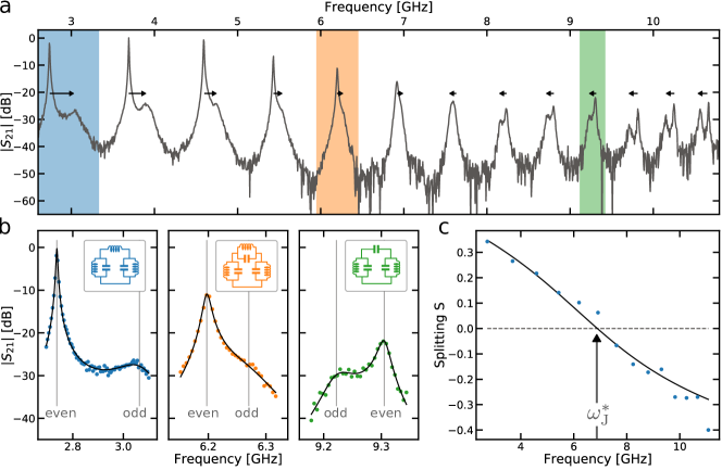
Figure 2: Inferring the renormalized resonant frequency $\omega_{\text{J}}^{*}$ of the small Josephson junction. a Amplitude of the microwave transmission $|S_{21}|$ versus frequency (sample A, 24mK). The even-odd modes frequency splitting $S$ changes sign precisely at $\omega_{\text{J}}^{*}$. Arrows are guides to the eye of the splitting sign. b Fit of the double peaks for three cases: well below the resonant frequency of the small Josephson junction (blue) its inductive part dominates, close to $\omega_{\text{J}}^{*}$ (orange) the impedance of the junction is large so that the two modes are almost decoupled, and well above $\omega_{\text{J}}^{*}$ (green) the capacitive part of the junction dominates. c Experimental normalized frequency splittings $S$ obtained from the previous fits (dots) and theoretical prediction (full line). The resonance frequency $\omega_{\text{J}}^{*}$ of the small Josephson junction corresponds to the vanishing value of the normalized splitting $S$.

Line shapes
The line shape of a given even-odd pair of resonances can be obtained by associating with it two effective LC oscillator Pozar (2009) connected via the small Josephson junction (see insets in figure 2b). In the regime of interest (See Supplementary Note 5 and 6) this junction can be treated as a ZPF-dependent inductance $L_{\text{J}}^{*}$ in parallel with a capacitance $C_{\mathbin{\!/\mkern-5.0mu/\!}}$, with resonance frequency $\omega_{\text{J}}^{*}=1/\sqrt{L_{\text{J}}^{*}C_{\mathbin{\!/\mkern-5.0mu/\!}}}$. The odd and even modes mentioned earlier are characterized by respective frequencies $\omega_{\text{even}}=1/\sqrt{LC}$ and $\omega_{\text{odd}}=1/\sqrt{L_{\Sigma}C_{\Sigma}}$, with $1/L_{\Sigma}=1/2L+1/L_{\text{J}}^{*}$ and $C_{\Sigma}=C/2+C_{\mathbin{\!/\mkern-5.0mu/\!}}$. Then for modes at frequencies such that $\omega_{\text{odd}},\omega_{\text{even}}\ll\omega_{\text{J}}^{*}$, the capacitance of the small junction can be neglected ($C_{\mathbin{\!/\mkern-5.0mu/\!}}\sim 0$) leading to $\omega_{\text{odd}}>\omega_{\text{even}}$. In the opposite case ($\omega_{\text{odd}},\omega_{\text{even}}\gg\omega_{\text{J}}^{*}$) the inductance can be neglected, giving $\omega_{\text{odd}}<\omega_{\text{even}}$. The most interesting regime is when the system is probed close to $\omega_{\text{J}}^{*}$. In that case, the impedance of the small junction diverges and consequently the two effective oscillators are uncoupled leading to $\omega_{\text{odd}}=\omega_{\text{even}}$. In the Supplementary Note 7, we confirm that a fully microscopic model of the whole circuit also predicts that the frequency splitting between even and odd modes changes sign at the renormalized frequency of the junction $\omega_{\text{J}}^{*}$. The frequencies of each even-odd pair of modes is extracted by fitting the peaks Fig. 2 to line shapes of an input-output formalism based on the simple model just described (see Supplementary Figure 3 and Methods).

Renormalized Josephson energy $E_{\text{J}}^{*}$
The effective resonance frequency of the junction, $\omega_{\text{J}}^{*}$, depends on its environment due to the interplay of strong anharmonicity and many-body ZPF, and can be inferred by tracking the evolution of the normalized frequency splitting $S=(\omega_{\text{odd,k}}-\omega_{\text{even,k}})/(\omega_{\text{even,k+1}}-\omega_{\text{even,k}})$, between even (uncoupled) and odd (coupled) modes, where $\text{k}=0\ldots M$ refers to mode number. As shown in Ref.  Puertas Martinez et al. (2019), in a long chain, this quantity equals the phase shift difference between even and odd modes. It vanishes when the left and right halves of the device decouple, so that even and odd modes become degenerate. Figure 2.c shows the experimentally obtained $S$ for one of our samples, from which we extract $\omega_{\text{J}}^{*}$. As we show in the Supplementary Note 4 and 5, the ZPF-dependent effective inductance of the weak link is related to a renormalized Josephson energy $E_{\text{J}}^{*}=(\hbar/2e)^{2}/L_{\text{J}}^{*}$ as

$$\omega_{\text{J}}^{*}=\sqrt{2E_{\text{J}}^{*}E_{\text{c}}},$$ (1)

where $E_{\text{c}}=(2e)^{2}/(2(C_{\text{J}}+C_{\text{sh}}))$, with $C_{\text{J}}$ the intrinsic capacitance of the junction and $C_{\text{sh}}$ a shunting capacitance due to the surrounding circuitry. Note that we define $E_{\text{J}}^{*}$ in terms of $L_{\text{J}}^{*}$, and not in terms of the DC critical current as is done in for instance Hekking and Glazman (1997). We use Eq. (1) to infer $E_{\text{J}}^{*}$ experimentally. $C_{\text{J}}$ is given by the junction size measured from an SEM picture. The way $C_{\text{sh}}$ is extracted is explained in the Supplementary Note 9. Values for sample A, B and C are reported in table 1. To see the effect of vacuum fluctuations, we compare $E_{\text{J}}^{*}$ to the bare Josephson energy of the weak link, which was obtained as follows. We fabricated many nominally identical Josephson junctions on the same chip and measured their room temperature resistances. The expected bare Josephson energy of the small Josephson junction $E_{\text{J,bare}}^{\text{AB}}$ (see table 1) was then inferred using the Ambegaokar-Baratoff law. We observe a systematic shift between this bare energy and the renormalized one we inferred from $|S_{21}|$ measurements, a shift that is more pronounced for sample A that shows a high non-linearity. This points towards a large renormalization induced by the strong zero-point phase fluctuations of the hybridyzed junction-chain modes, as expected since the small junction is impedance-matched to the chains.

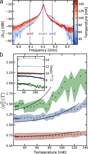
Figure 3: Temperature-induced renormalization. a Zoom on a even-odd pair of transmission peaks for sample A at temperature ranging from 23 to 150 mK. The even mode (gray) does not move while the odd mode (blue is at 25mK, red at 130mK) shift down in frequency when warming up, showing a downward renormalization of the junction frequency $\omega_{\text{J}}^{*}$. b ZPF of the small junction $\expectationvalue{\phi_{\text{J}}^{2}}$ as a function of the temperature for three samples (A,B and C ranging from dark to light blue), extracted from Eq. (2). ZPF are stronger in sample A, which is associated to a smaller ratio $E_{\text{J,bare}}/E_{\text{c}}$ (large non-linearity). The measured quantum to classical crossover is in good agreement with theory (full lines). The inset displays the corresponding renormalised junction frequency $f_{\text{J}}^{*}=\omega_{\text{J}}^{*}/2\pi$ of the three samples. The full lines are the SCHA predictions while the dashed lines represent what would be the temperature evolution of these frequencies if ZPF were omitted from $\expectationvalue{\phi_{\text{J}}^{2}}$, using the same values of $E_{\text{J,bare}}$.

We now show that this renormalization is quantitatively captured by a microscopic model based on the self consistent harmonic approximation (SCHA). Its success in accounting for nonlinearities introduced by Josephson junctions is well-established Zaikin and Panyukov (1986); Panyukov and Zaikin (1988); Kampf and Schön (1987); Chakravarty et al. (1988). More recently it was employed in detailed microscopic models in the field of circuit-QED Puertas Martinez et al. (2019); Joyez (2013). The idea behind the SCHA is that the strong phase fluctuations allowed by the environment average the non-linear potential of the small Josephson junction, lowering its effective Josephson energy from the bare value $E_{\text{J}}$ to the renormalized one $E_{\text{J}}^{*}$. This is valid, provided the phase $\phi_{\text{J}}$, though strongly fluctuating, is still sufficiently localized. In this regard we note the following. Though large, the effective environmental impedence $2Z_{\text{chain}}\simeq$$3.8\text{\,}\mathrm{k\SIUnitSymbolOhm}\text{/}$ seen by the weak link, is still less than $R_{\text{Q}}$. Under this condition, the environment is known to produce spontaneous symmetry breaking of the 2$\pi$ periodicity in the phase difference $\phi_{\text{J}}$ across the weak link, Schmid (1983); Bulgadaev (1984); Schön and Zaikin (1990). It is therefore reasonable to approximate the system’s full wave function with a Gaussian that is fairly well localized in the $\phi_{\text{J}}$ direction, which is the essence of the SCHA. At zero temperature, the interplay of many-body ZPF and non-linearity can be described is approximated by replacing the cosine Josephson potential by an effective quadratic term $E_{\text{J}}^{*}\phi_{\text{J}}^{2}/2$, where the renormalized Josephson energy $E_{\text{J}}^{*}$ is given by the self-consistent equation:

$$E_{\text{J}}^{*}=E_{\text{J,bare}}\,e^{-\expectationvalue{\phi_{\text{J}}^{2}(E_{\text{J}}^{*})}/2}.$$ (2)

Here, the total phase fluctuation across the junction $\expectationvalue{\phi_{\text{J}}^{2}}$ is given by:

$$\expectationvalue{\phi_{\text{J}}^{2}}=\sum_{k\in\text{odd}}{\phi_{k}^{2}},$$ (3)

where $\phi_{k}^{2}$ is the contribution to the small junction ZPF coming from odd mode $k$. Importantly, in the strong ZPF regime, the expectation value must be taken with respect to the modified vacuum of the hybridized modes, which means that the normal modes of the systems has to be updated during the numerical iteration of Eq. (2). This is in contrast to familiar examples of ZPF induced phenomena, such as the Lamb shift in hydrogen, where the perturbative nature of the effect allows one to calculate fluctuations with respect to the bare vacuum of the environment. We independently extracted the parameters of the whole circuit (junction+chains), and then used Eq. (2) to determine the theoretical bare Josephson energy required to find back the measured renormalized $E_{\text{J}}^{*}$ (see next section for more details). The agreement between experimentally and theoretically estimated $E_{\text{J,bare}}$ (see table 1) provides strong evidence that our system displays large ZPF, which leads to a renormalization of up to $50\%$ of the Josephson energy of the small junction (or equivalently $30\%$ of its resonant frequency $\omega_{\text{J}}$). Moreover, as expected, this renormalization increases when the ratio $E_{\text{J,bare}}/E_{\text{c}}$ decreases, or equivalently when the non-linearity of the small Josephson junction increases.

Quantum versus thermal fluctuations
As $\omega_{\text{J}}^{*}$ is renormalized by phase fluctuations across the weak link, one expects a crossover from quantum to thermally driven fluctuations as temperature increases. Extending the SCHA to non-zero temperatures (see Supplementary Note 4 and 5), we find that the fluctuations of mode $k$ contain a Bose factor contribution:

$$\phi_{k}^{2}(T)=\phi_{k}^{2}\left[1+\frac{2}{\mathrm{exp}(\hbar\omega_{k}/k_{\text{B}}T)-1}\right]$$ (4)

with $\omega_{k}$ the frequency of mode $k$, and $\phi_{k}^{2}$ its zero temperature ZPF. Therefore, at low temperature, fluctuations saturate to a finite ZPF value (a hallmark of quantum uncertainty), while at high temperature they increase linearly with temperature (4). According to Eq. (2), $\omega_{\text{J}}^{*}$ should decrease when the system is heated up. Consequently, odd modes’ frequencies are shifted to lower values when temperature increases, while the even modes stay put. This striking experimental signature of non-linearity can clearly be seen in 3.a. This constitutes smoking gun evidence of the back-action of the Josephson junction on its environment: the shift of $\omega_{\text{J}}^{*}$ to smaller values at increasing temperatures indicates that fluctuations are thermally enhanced.

The recipe to extract $E_{\text{J,bare}}^{\text{th}}$ is the following: $E_{\text{J}}^{*}(T)$ is obtained from $S_{21}$ measurements at different temperatures. Since all the other parameters ($L$, $C$, $C_{\text{g}}$, $C_{\text{J}}$ and $C_{\text{sh}}$) are known, we can fit $E_{\text{J}}^{*}(T)$ using Eqs. (2) and (4), taking $E_{\text{J,bare}}^{\text{th}}$ as the (only) fitting parameter. Then, $E_{\text{J,bare}}^{\text{th}}$ being determined, we can compute the phase fluctuations across the small Josephson junction using Eq. (1) and (2):

$$\expectationvalue{\phi_{\text{J}}^{2}}(T)=4\log(\frac{2E_{\text{J,bare}}^{\text{th}}E_{\text{c}}}{\omega_{J}^{*}(T)}).$$ (5)

We checked that at the lowest temperature of our cryostat, the phase fluctuations experienced by the small Josephson junction are fully in the quantum regime, by measuring $|S_{\text{21}}|$ from 25mK to 130mK. Results are shown in figure 3.b. We observe that the quantum to classical crossover appears at decreasing temperatures from sample C to A. This is because $\omega_{\text{J}}^{*}$ decreases from sample C to A. Therefore the junction is coupled to modes with lower and lower frequencies, which are thermally occupied at lower temperatures. The inset in figure 3.b shows the corresponding fit of $\omega_{\text{J}}^{*}$ for the three samples. The dashed lines represent $\omega_{\text{J}}^{*}$ obtained using the value of $E_{\text{J,bare}}$ extracted from the previous fit but including only thermal renormalization of $\omega_{\text{J}}^{*}$ i.e. disregarding ZPF. Consequently, $\expectationvalue{\phi_{\text{J}}^{2}}$ is given by:

$$\phi_{k}^{2}(T)=\phi_{k}^{2}\left[\frac{2}{\mathrm{exp}(\hbar\omega_{k}/k_{\text{B}}T)-1}\right]$$ (6)

The discrepancy between the dashed lines and the fit clearly shows that the fluctuations have mainly quantum origin. At increasing temperatures, thermal fluctuations add up to the quantum ZPF, and cause a rise in $\big{<}\phi_{\text{J}}^{2}\big{>}$, witnessed both in the experimental extraction and the predictions from SCHA, see figure 3b. It is likely that the extracted $\big{<}\phi_{\text{J}}^{2}\big{>}$ for sample A is systematically underestimated due to sizeable errors in the SCHA that rapidly set in after $\big{<}\phi_{\text{J}}^{2}\big{>}\gtrsim 1$, leading to a mismatch with the theory at high temperatures.

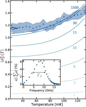
Figure 4: Many-body nature of the ZPF. Total phase fluctuations across the small Josephson junction in sample B, taking into account in our model (full lines) different numbers of modes of the environment, ranging from one (light blue) to the total number (dark blue). The inset shows the relative contribution of the different modes to the total fluctuations, with $\Gamma_{\text{J}}$ being the FWHM of this quantity.

Many-body nature of the ZPF
In order to confirm the many-body character of this renormalization, we can estimate how many modes are affecting the small junction simultaneously. The ZPF are quantitatively determined by how the full vacuum of the whole circuit is dressed by the coupling through the weak-link. Within the SCHA, the number of modes contributing a finite amount of $\phi_{k}^{2}$ provides a measure of the number of interacting particles in the system. In figure 4. we compare the experimentally extracted $\expectationvalue{\phi_{\text{J}}^{2}(T)}$ to various calculated values. In each calculation, the full system was truncated to a finite number of modes in a window around $\omega_{\text{J}}^{*}$. If the window is too narrow, important contributions to the ZPF are neglected, and $\expectationvalue{\phi_{\text{J}}^{2}(T)}$ is underestimated. The comparison unambiguously shows that, in sample B, around 30 modes contribute to the total phase fluctuations. In circuit QED language, the full width at half maximum (FWHM) of the environmental ZPF $\phi_{\text{k}}^{2}(\omega_{\text{k}})$ – labeled $\Gamma_{\text{J}}$ – is about 7GHz for our samples (see inset of figure 4.). Therefore, our device operates in a regime where $\Gamma_{\text{J}}/\omega_{\text{J}}^{*}\sim 1$ due to the impedance matching to the transmission line. Moreover, our device is strongly non-linear. Consequently, it is not possible to treat perturbatively the non-linearity as is usually done in the field for the Transmon qubit or other weakly non-linear circuits Koch et al. (2007); Nigg et al. (2012); Bourassa et al. (2012); Weissl et al. (2015a) (a detailed analysis is given in Supplementary Note 11).

This work provides a direct observation of several quantum many-body effects driven by zero point fluctuations in an open quantum system. This was achieved by developing a spectroscopic setup where the high-impedance environment of a single non-linear Josephson junction was monitored mode by mode, and compared to a detailed microscopic model. A strong quantum renormalization (up to 50%) of the Josephson energy of the single junction was demonstrated, analogous to a non-perturbative Lamb shift. In addition, the back-action of the small Josephson junction causes non-linear broadening and strong temperature dependence of the environmental modes, providing the most striking signature of the many-body effects that take place in our circuit. The measured temperature dependence of the phase fluctuation across the Josephson junction indicates that our device remains quantum coherent at cryogenic temperatures. As many as 30 modes are involved in the renormalization of the small junction. Our superconducting circuit thus behaves as a fully fledged quantum many body simulator, paving the way for the further observation of various many-body non-linear effects in circuit-QED  Garcia-Ripoll et al. (2008); Le Hur (2012); Goldstein et al. (2013); Peropadre et al. (2013); Snyman and Florens (2015); Gheeraert et al. (2017, 2018).

Correspondence
Correspondence and requests for materials should be addressed to Nicolas Roch (email: nicolas.roch@neel.cnrs.fr).

Methods

Full Model
The Hamiltonian of the full system can be decomposed into odd and even parts – containing respectively the modes coupled and not coupled to the junction (see Supplementary Note 2). The odd Hamiltonian reads:

$$\hat{H} = \hat{H}_{0}+\left(1-E_{\text{J,bare}}\cos\hat{\phi}_{\text{J}}\right),$$ (7)

$$\hat{H}_{0} = \frac{\left(2e\right)^{2}}{2}\sum_{i,j=0}^{N}{\hat{n}_{i}\big{[}\hat{C}\big{]}^{-1}_{i,j}\hat{n}_{j}}+\frac{E_{\text{J,S}}}{4}\sum_{i=1}^{N-1}{\left(\hat{\phi}_{i}-\hat{\phi}_{i+1}\right)^{2}},$$ (8)

with $\hat{n}_{0}\equiv\hat{n}_{J}$ and $\hat{\phi}_{\text{J}}$ referring to the charge the phase drop across the small junction while $\hat{n}_{i}$ and $\hat{\phi}_{i}$, $i\in[1..N]$ refer to the charge and phase operators on chain site $i\in[1..N]$. Charge and phase operators obey the commutation rules $\big{[}\hat{\phi}_{k},\hat{n}_{p}\big{]}=i\delta_{k,p}$. The microscopic parameters are $E_{\text{J,S}}$, the Josephson energy of the SQUIDs, $E_{\text{J,bare}}$ the bare Josephson energy of the small junction, and the capacitance matrix:

$$\hat{C}=\frac{1}{2}\begin{bmatrix}C_{I}&-C&0&0&0&\dots&0\\ -C&2C+C_{g}&-C&0&0&\dots&0\\ 0&-C&2C+C_{g}&-C&0&\dots&0\\ \vdots&\vdots&\ddots&\ddots&\ddots&\dots&0\\ 0&0&0&-C&2C+C_{g}&-C&0\\ 0&0&0&0&-C&2C+C_{g}&-C\\ 0&0&0&0&0&-C&C_{0}\\ \end{bmatrix}$$

with :

$$C_{I} =2(C_{\text{J}}+C_{\text{sh}})+C+C_{\text{g}},$$ (9)

$$C_{0} =C_{\text{c}}+C_{\text{c,I}}+C.$$ (10)

Self Consistent Harmonic Approximation (SCHA)
Because of the cosine term in Eq. (7), we are dealing with an interacting many-body problem that cannot be solved analytically. To study the best variational harmonic approximation we use the SCHA:

$$\hat{H} =\hat{H}_{0}+\frac{E^{*}_{\text{J}}}{2}\hat{\phi}_{\text{J}}^{2}+\left(1-E_{\text{J,bare}}\cos\hat{\phi}_{\text{J}}\right)-\frac{E^{*}_{\text{J}}}{2}\hat{\phi}_{\text{J}}^{2}$$ (11)

$$=\hat{H}_{\text{t}}+\left(1-E_{\text{J,bare}}\cos\hat{\phi}_{\text{J}}\right)-\frac{E^{*}_{\text{J}}}{2}\hat{\phi}_{\text{J}}^{2},$$ (12)

with $\hat{H}_{\text{t}}$ the trial harmonic Hamiltonian that will approximate $\hat{H}$, optimized with respect to the renormalized Josephson energy $E^{*}_{\text{J}}$. The variational principle gives:

$$\frac{\partial}{\partial E^{*}_{\text{J}}}\expectationvalue{\hat{H}}{\Psi_{\text{t}}}=0,$$ (13)

with $\ket{\Psi_{\text{t}}}$ the many-body ground state of $\hat{H}_{\text{t}}$. Because of the harmonic character of $\hat{H}_{\text{t}}$, we have:

$$\expectationvalue{\cos\hat{\phi}_{\text{J}}}{\Psi_{\text{t}}}=e^{-\expectationvalue{\hat{\phi}_{\text{J}}^{2}}{\Psi_{\text{t}}}/2}.$$ (14)

Inserting (14) into (13) we end up with the self consistent equation:

$$E_{\text{J}}^{*}=E_{\text{J,bare}}e^{-\expectationvalue{\phi_{\text{J}}^{2}(E_{\text{J}}^{*})}_{\text{t}}/2}.$$ (15)

The physical interpretation is the following: when ZPF are negligible, $\big{<}\hat{\phi}_{\text{J}}^{2}\big{>}\simeq 0$ and $E_{\text{J}}^{*}=E_{\text{J,bare}}$, so in its ground state the junction behaves as an harmonic oscillator of frequency $\omega_{\text{J,bare}}=\sqrt{2E_{\text{J,bare}}E_{\text{c}}}$. For weak non-linearity, fluctuations increase but remain such that $\big{<}\hat{\phi}_{\text{J}}^{2}\big{>}\ll 1$, resulting in $E_{\text{J}}^{*}\simeq E_{\text{J,bare}}(1-\big{<}\phi_{\text{J}}^{2}\big{>}/2)$, so that the junction behaves as a weakly anharmonic oscillator with fundamental frequency $\omega_{\text{J,bare}}(1-\big{<}\hat{\phi}_{\text{J}}^{2}\big{>}/4)$. For an isolated junction $\big{<}\hat{\phi}_{\text{J}}^{2}\big{>}=\sqrt{E_{\text{c}}/2E_{\text{J,bare}}}$, and the frequency becomes $\omega_{\text{J,bare}}-E_{\text{c}}/4$, a well known result for the Transmon qubit Koch et al. (2007). For larger fluctuations, the principle remains the same but no analytical formula can be derived, so that one should solve the self consistent equation numerically. A more detailed derivation – including thermal fluctuations – is presented in Supplementary Note 4 and 5.

Frequency splitting S between odd and even modes
The splitting $S$ is linked to the phase shift difference $\theta$ between even and odd modes in the thermodynamic limit Puertas Martinez et al. (2019):

$$S=\frac{\theta}{\pi}.$$ (16)

The analytical formula of the phase shift difference– derived in the Supplementary 6 and 7 – reads :

$$\theta=2\,{\rm arccot}(X)+{\rm arctan}\left[\frac{1-\lambda}{1+\lambda}X\right]$$ (17)

with

$$X =\sqrt{\left(\frac{4C}{C_{\text{g}}}+1\right)\left(\left(\frac{\omega_{\text{p}}}{\omega}\right)^{2}-1\right)},$$ (18)

$$\lambda =\frac{1-\omega^{2}CL}{1+2L/L_{\text{J}}^{*}-\omega^{2}C_{\text{I}}L},$$ (19)

$\omega_{\text{p}}=1/\sqrt{L(C+C_{\text{g}}/4)}$ being the plasma frequency of the chain and $L_{\text{J}}^{*}=\hbar^{2}/(2e)^{2}E_{\text{J}}^{*}$ the effective inductance of the small junction.

Fitting formula for the peaks
Input-output theory is used to fit the parameters associated to the double resonances observed in the transmission spectrum. These are mapped to two coupled harmonic modes $\alpha$ and $\beta$ with mutual coupling rate $g$, external coupling $\kappa_{\text{ext}}$ and internal loss $\kappa_{\text{in}}$, with Hamiltonian:

$$\hat{H}=\hbar\omega_{\text{r}}(\hat{a_{\text{L}}}^{\dagger}\hat{a_{\text{L}}}+{a_{\text{R}}}^{\dagger}\hat{a_{\text{R}}})+g(\hat{a_{\text{L}}}+\hat{a_{\text{L}}}^{\dagger})(\hat{a_{\text{R}}}+\hat{a_{\text{R}}}^{\dagger}).$$ (20)

Here $\hat{a}_{\text{in}_{\text{L}}}$,$\hat{a}_{\text{out}_{\text{L}}}$ are the left input and output signals and $\hat{a}_{\text{out}_{\text{R}}}$ is the right output signal. Thus the input-output relations are :

$$\hat{a}_{\text{in}_{\text{L}}}+\hat{a}_{\text{out}_{\text{L}}} =\sqrt{\kappa_{\text{ext}}}\hat{a_{\text{L}}},$$ (21)

$$\hat{a}_{\text{out}_{\text{R}}} =\sqrt{\kappa_{\text{ext}}}\hat{a_{\text{R}}}.$$ (22)

The equations of motion are:

$$-i(\omega-i\omega_{\text{r}})\hat{a_{\text{L}}}+\frac{\kappa_{\text{ext}}}{2}\hat{a_{\text{L}}} =-ig\hat{a_{\text{R}}}-\sqrt{\kappa_{\text{ext}}}\hat{a}_{\text{in}_{\text{L}}},$$ (23)

$$-i(\omega-i\omega_{\text{r}})\hat{a_{\text{R}}}+\frac{\kappa_{\text{ext}}}{2}\hat{a_{\text{R}}} =-ig\hat{a_{\text{L}}}.$$ (24)

The complex transmission is defined as $S_{21}=\hat{a}_{\text{out}_{\text{R}}}/\hat{a}_{\text{in}_{\text{L}}}$, and can be calculated using Eqs. (21-24). We define the even $\omega_{\text{e}}=\omega_{\text{r}}+g$ and odd $\omega_{\text{o}}=\omega_{\text{r}}-g$ frequencies, and add phenomenologically losses in the odd modes $\kappa_{\text{o}}=\kappa_{\text{in}}+\kappa_{\text{add}}$ (we keep $\kappa_{\text{e}}=\kappa_{\text{in}}$), so that:

$$S_{21}=\frac{i\kappa_{\text{ext}}(\omega_{\text{o}}-\omega_{\text{e}})}{\left(\kappa_{\text{ext}}+\kappa_{\text{o}}+-2i(\omega-\omega_{\text{o}})\right)\left(\kappa_{\text{ext}}+\kappa_{\text{e}}-2i(\omega-\omega_{\text{e}})\right)}.$$ (25)

For some of the odd modes, we found a signature of inhomogeneous broadening, that we modeled by a convolution of their frequency with a gate function defined as $\Pi_{\delta\omega}(\omega)=1/\delta\omega$ if $\omega\in[\omega-\delta\omega/2,\omega+\delta\omega/2]$. Understanding microscopically this additional broadening, possibly due to offset charges, is beyond the scope of the description using the SCHA, and will require additional theoretical developments.

Data Availability
The data that support the findings of this study are available from the corresponding author upon reasonable request.

Acknowledgements
The authors would like to thank F. Balestro, L. Del Rey, D. Dufeu, E. Eyraud, J. Jarreau, T. Meunier and W. Wernsdorfer, for early support with the experimental setup. Very fruitful discussions with K. R. Amin, P. Forn-Diaz, J.-J. Garcia-Ripoll, D. B. Haviland, M. Houzet, P. Joyez, V. E. Manucharyan, F. Portier and H. E. Tureci are acknowledged. The sample was fabricated in the Nanofab clean room. This research was supported by the ANR under contracts CLOUD (project number ANR-16-CE24-0005), GEARED (project number ANR-14-CE26-0018), by the National Research Foundation of South Africa (Grant No. 90657), and by the PICS contract FERMICATS. J.P.M. acknowledges support from the Laboratoire d’excellence LANEF in Grenoble (ANR-10-LABX-51-01). R.D. and S.L. acknowledge support from the CFM foundation and the ’Investisements d’avenir’ (ANR-15-IDEX-02) programs of the French National Research Agency. K.B. and J.D. acknowledge the European Union’s Horizon 2020 research and innovation programme under the Marie Sklodowska-Curie grant agreement No 754303.

Competing interests
The authors declare no competing financial or non-financial interests.

Author contributions
S.L., J.P.M., S.F. and N.R. designed the experiment. S.L. fabricated the device. S.L. performed the experiment and analysed the data with help from S.F., N.R. and I.S., while S.F. and I.S. provided the theoretical support. S.L., J.P.M., K.B., R.D., J.D., F.F., V.M., L.P., O.B., C.N., W.H.G., S.F., I.S. and N.R. participated in setting up the experimental platform, and took part in writing the paper.

Supplementary information for "Observation of quantum many-body effects due to zero point fluctuations in superconducting circuits”

.1 Supplementary Note 1: Experimental setup

The measurement setup is displayed in Supplementary Figure S1. The samples are put in a dilution refrigerator with a 25mK base temperature. $|S_{21}|$ is measured using a Vector Network Analyzer (VNA). An additional microwave source was used for two-tone measurements, while a global magnetic field was applied via an external superconducting coil. Both the coil and the sample were held inside a mu-metal magnetic shield coated on the inside with a light absorber made out of epoxy loaded with silicon and carbon powder. IR filters are 0.40mm thick stainless steel coaxial cables. The bandwidth of the measurement setup goes from 2.5 GHz to 12 GHz.

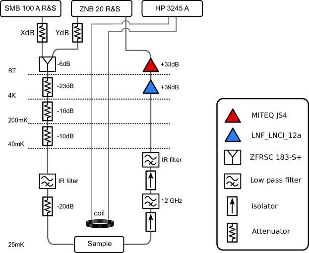
Figure S1: Measurement setup.

.2 Supplementary Note 2: Odd and Even modes

Our device consists of two long Josephson chains of $N+1$ sites tailored in the linear regime (with Josephson energy $(\hbar/2e)^{2}/L$ much larger than the capacitive energy) interconnected via a smaller Josephson junction or weak-link (operating in the regime of small Josephson energy $E_{J,\text{bare}}$). Linearizing the tunneling term within each chain, but keeping the non-linear coupling between them, the Hamiltonian of the system reads:

$$\hat{H}=\frac{\left(2e\right)^{2}}{2}\sum_{i,j=0}^{N}\sum_{\sigma,\sigma^{\prime}\in L,R}{\hat{n}_{i\sigma}[C]^{-1}_{i,\sigma,j,\sigma^{\prime}}\hat{n}_{j,\sigma^{\prime}}}+\frac{1}{2}\frac{\hbar^{2}}{(2e)^{2}L}\sum_{i=1}^{N-1}\sum_{\sigma\in L,R}{\left(\hat{\phi}_{i,\sigma}-\hat{\phi}_{i+1,\sigma}\right)^{2}}-E_{J,\text{bare}}\cos\left(\hat{\phi}_{0,L}-\hat{\phi}_{0,R}\right),$$ (S1)

with $\hat{n}_{i,\sigma}$ and $\hat{\phi}_{i,\sigma}$ the charge and phase operators on site $i\in[1..N]$ and in chain $\sigma=L,R$. These operators are canonically conjugate and obey at the quantum mechanical level the commutation rules $\big{[}\hat{\phi}_{i,\sigma},\hat{n}_{j,\sigma^{\prime}}\big{]}=i\delta_{i,j}\delta_{\sigma,\sigma^{\prime}}$. The capacitance matrices can be read off the equivalent circuit in Supplementary Figure S2, and are decomposed into an intra-chain part $[C_{0}]=[C]_{LL}=[C]_{RR}$ and an interchain part intra-chain part $[C_{1}]=[C]_{LR}=[C]_{RL}$, which read explicitely:

$$[C_{0}]=\begin{bmatrix}C_{\text{I}}&-C&0&0&0&\dots&0\\ -C&2C+C_{\text{g}}&-C&0&0&\dots&0\\ 0&-C&2C+C_{\text{g}}&-C&0&\dots&0\\ \vdots&\vdots&\ddots&\ddots&\ddots&\dots&0\\ 0&0&0&-C&2C+C_{\text{g}}&-C&0\\ 0&0&0&0&-C&2C+C_{\text{g}}&-C\\ 0&0&0&0&0&-C&C_{\text{O}}\\ \end{bmatrix},$$

and $[C_{1}]_{i,j}=-\delta_{0,i}\delta_{j,0}(C_{\text{J}}+C_{\text{sh}})$ with $(i,j)\in[0,N]^{2}$. The total capacitance at the weak-link end of the chain amounts to $C_{\text{I}}=C_{\text{J}}+C_{\text{sh}}+C+C_{\text{g}}$, while the capacitance at the connecting output port is $C_{\text{O}}=C_{\text{c}}+C_{\text{c,I}}+C$.

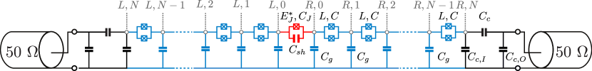
Figure S2: Electrical circuit of the device. The capacitance network is indicated for the output ports (in black), the two chains (in blue) and the weak link (in red).

Due to the symmetry of our device, it is useful to define respectively even and odd modes:

$$\hat{n}_{j,\pm} =\frac{1}{2}\left(\hat{n}_{j,R}\pm\hat{n}_{j,L}\right),$$ (S2)

$$\hat{\phi}_{j,\pm} =\left(\hat{\phi_{j,R}}\pm\hat{\phi_{j,L}}\right).$$ (S3)

In this basis, the Hamiltonian decomposes in two uncoupled subsystems: $\hat{H}=\hat{H}_{+}+\hat{H}_{-}$, where:

$$\hat{H}_{+} =\frac{\left(2e\right)^{2}}{2}\sum_{i,j=0}^{N}{\hat{n}_{i,+}\left[\frac{C_{0}+C_{1}}{2}\right]^{-1}_{i,j}\hat{n}_{j,+}}+\frac{1}{4}\frac{\hbar^{2}}{(2e)^{2}L}\sum_{i=1}^{N-1}{\left(\hat{\phi}_{i,+}-\hat{\phi}_{i+1,+}\right)^{2}},$$ (S4)

$$\hat{H}_{-} =\frac{\left(2e\right)^{2}}{2}\sum_{i,j=0}^{N}{\hat{n}_{i,-}\left[\frac{C_{0}-C_{1}}{2}\right]^{-1}_{i,j}\hat{n}_{j,-}}+\frac{1}{4}\frac{\hbar^{2}}{(2e)^{2}L}\sum_{i=1}^{N-1}{\left(\hat{\phi}_{i,-}-\hat{\phi}_{i+1,-}\right)^{2}}+E_{\text{J}}\left(1-\cos\hat{\phi}_{0,-}\right).$$ (S5)

$\hat{H}_{+}$ reduces to the Hamiltonian of a linear chain, while $\hat{H}_{-}$ takes the form of a boundary Sine-Gordon-like model.

.3 Supplementary Note 3: Fitting the transmission resonances

The transmission spectrum consists of pairs of peaks, that are fitted according to the model described in the Methods section of the main text. Close to a pair of even/odd resonances, the transmission is given by the formula:

$$S_{21}=\frac{i\kappa_{\text{ext}}(\omega_{\text{o}}-\omega_{\text{e}})}{\left(\kappa_{\text{ext}}+\kappa_{\text{o}}+-2i(\omega-\omega_{\text{o}})\right)\left(\kappa_{\text{ext}}+\kappa_{\text{e}}-2i(\omega-\omega_{\text{e}})\right)},$$ (S6)

with $\omega_{\text{o}}$ and $\omega_{\text{e}}$ the even/odd resonance frequencies, $\kappa_{\text{e}}$ and $\kappa_{\text{o}}$ their respective intrinsic damping rate, and $\kappa_{\text{ext}}$ the broadening due to the 50 $\Omega$ output ports. A large selection of fitted spectra (for all three samples and various temperatures) is shown in Supplementary Figure S3.

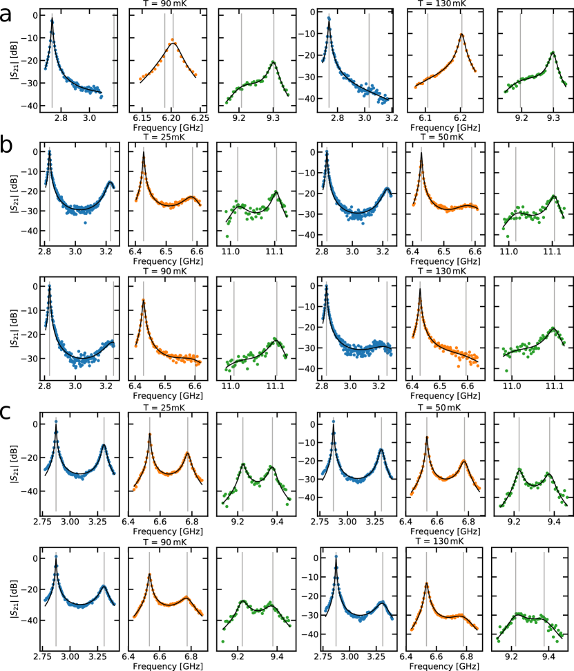
Figure S3: Fitting of various peak pairs. Panel a is for sample 300, panel b is for sample 375 and panel c is for sample 450. Various temperature choices are indicated, and for each case, three frequencies ranges are indicated (in blue, orange and green respectively). Vertical grey lines are the positions of the resonance pairs found by the regression (black lines) using formula (S6).

.4 Supplementary Note 4: The self consistent harmonic approximation

The hamiltonian $\hat{H}_{-}$ describes a quantum many-body problem that cannot be solved analytically, and we therefore develop here an approximate yet microscopic approach to the problem. From now on, we will discard the - index in all fields, and replace $\hat{\phi}_{0,-}$ by $\hat{\phi}_{\text{J}}$. The self consistent harmonic approximation (SCHA) is used to find the approximate ground state at thermal equilibrium Joyez (2013); Puertas Martinez et al. (2019). This method consist of finding the best harmonic Hamiltonian $\hat{H}_{\text{t}}$ which satisfies the Gibbs-Bogoliubov inequality $F\leq F_{\text{t}}+\langle\hat{H}-\hat{H}_{\text{t}}\rangle_{\text{t}}$, where:

$$F_{\text{t}} =-k_{\text{B}}T\ln Z_{\text{t}},$$ (S7)

$$Z_{\text{t}} =\tr(e^{-\hat{H}_{\text{t}}/k_{\text{B}}T}),$$ (S8)

$$\langle\hat{H}-\hat{H}_{\text{t}}\rangle_{\text{t}} =\tr((\hat{H}-\hat{H}_{\text{t}})\hat{\rho}_{\text{t}}),$$ (S9)

$$\hat{\rho}_{\text{t}} =\frac{1}{Z_{\text{t}}}e^{-\hat{H}_{\text{t}}/k_{\text{B}}T}.$$ (S10)

The trial Hamiltonian $\hat{H}_{\text{t}}$ is defined by replacing in $\hat{H}$ the non-linear tunneling term $-E_{\text{J}}\cos\hat{\phi}_{\text{J}}$ by a renormalized potential $E_{\text{J}}^{*}\hat{\phi}_{\text{J}}^{2}/2$. The physical reason is that the zero point fluctuations of the small junction explore a large part of the Josephson potential, which amounts in first approximation to lower its effective Josephson energy from the bare value $E_{\text{J}}$ to a renormalized value $E_{\text{J}}^{*}$. Explicitely, the trial Hamiltonian reads:

$$\hat{H}_{\text{t}}=\frac{\left(2e\right)^{2}}{2}\sum_{i,j=0}^{N}{\hat{n}_{i}[C]^{-1}_{i,j}\hat{n}_{j}}+\frac{1}{2}\frac{\hbar^{2}}{(2e)^{2}}\sum_{i,j=0}^{N}{\hat{\phi}_{i}[L^{-1}]_{i,j}\hat{\phi}_{j}},$$ (S11)

with the capacitance matrix:

$$[C]=\frac{1}{2}\begin{bmatrix}C_{\Sigma}&-C&0&0&0&\dots&0\\ -C&2C+C_{\text{g}}&-C&0&0&\dots&0\\ 0&-C&2C+C_{\text{g}}&-C&0&\dots&0\\ \vdots&\vdots&\ddots&\ddots&\ddots&\dots&0\\ 0&0&0&-C&2C+C_{\text{g}}&-C&0\\ 0&0&0&0&-C&2C+C_{\text{g}}&-C\\ 0&0&0&0&0&-C&C_{\text{O}}\\ \end{bmatrix},$$

where $C_{\Sigma}=C_{\text{I}}+C_{\text{J}}+C_{\text{sh}}=2(C_{\text{J}}+C_{\text{sh}})+C+C_{\text{g}}$, and inductance matrix:

$$[L^{-1}]=\frac{1}{2}\begin{bmatrix}2/L^{*}+1/L&-1/L&0&0&0&\dots&0\\ -1/L&2/L&-1/L&0&0&\dots&0\\ 0&-1/L&2/L&-1/L&0&\dots&0\\ \vdots&\vdots&\ddots&\ddots&\ddots&\dots&0\\ 0&0&0&-1/L&2/L&-1/L&0\\ 0&0&0&0&-1/L&2/L&-1/L\\ 0&0&0&0&0&-1/L&1/L\\ \end{bmatrix}.$$

Here $L^{*}=(\hbar/2e)^{2}/E_{\text{J}}^{*}$ is an effective inductance associated with the weak link.

Let us define by $E_{k}=\hbar\omega_{k}$ the eigenvalues of $\hat{H}_{\text{t}}$ and $\hat{a}_{k}^{\dagger}$ the corresponding creation operators associated to its normal modes. As $\hat{H}_{\text{t}}$ is harmonic, one can write:

$$\hat{H}_{\text{t}} =\sum_{k=0}^{N+1}{\hbar\omega_{k}\hat{a}_{k}^{\dagger}\hat{a}_{k}},$$ (S12)

$$\hat{\phi}_{\text{J}} =\sum_{k=0}^{N+1}{\phi_{k}(\hat{a}_{k}^{\dagger}+\hat{a}_{k})}.$$ (S13)

The renormalized Josephson energy $E_{\text{J}}^{*}$ is obtained by minimizing the variational free energy:

$$\frac{d}{dE_{\text{J}}^{*}}(F_{\text{t}}+\langle\hat{H}-\hat{H}_{\text{t}}\rangle_{\text{t}})=0.$$ (S14)

The first term is evaluated as follows:

$$\dfrac{dF_{\text{t}}}{dE_{\text{J}}^{*}} =-\frac{k_{\text{B}}T}{Z_{\text{t}}}\dfrac{dZ_{\text{t}}}{dE_{\text{J}}^{*}}=-\frac{k_{\text{B}}T}{Z_{\text{t}}}\sum_{k}{\dfrac{d}{dE_{\text{J}}^{*}}\left(e^{-E_{k}/k_{\text{B}}T}\right)}=\frac{1}{Z_{\text{t}}}\sum_{k}\bra{k}\dfrac{d\hat{H}_{\text{t}}}{dE_{\text{J}}^{*}}\ket{k}e^{-E_{k}/k_{\text{B}}T}$$ (S15)

$$=\frac{1}{Z_{\text{t}}}\sum_{k}{\bra{k}\frac{\hat{\phi}_{\text{J}}^{2}}{2}\ket{k}e^{-E_{k}/k_{\text{B}}T}}=\frac{\langle\hat{\phi}_{\text{J}}^{2}\rangle_{\text{t}}}{2}$$ (S16)

where we used the fact that $\bra{k}\hat{H}_{\text{t}}\dfrac{d}{dE_{\text{J}}^{*}}\ket{k}=0$, which follows because $\ket{k}$ is a normalized eigenstate of $\hat{H}_{\text{t}}$ and $\dfrac{d}{dE_{\text{J}}^{*}}\ket{k}$ is orthogonal to $\ket{k}$. The second term in the variational free energy is

$$\frac{d}{dE_{\text{J}}^{*}}\langle\hat{H}-\hat{H}_{\text{t}}\rangle_{\text{t}}=-\frac{E_{\text{J},\text{bare}}}{2}\dfrac{d}{dE_{\text{J}}^{*}}\langle e^{i\hat{\phi}_{\text{J}}}+e^{-i\hat{\phi}_{\text{J}}}\rangle_{\text{t}}-\frac{\langle\hat{\phi}_{\text{J}}^{2}\rangle_{\text{t}}}{2}-\frac{E_{\text{J}}^{*}}{2}\dfrac{d}{dE_{\text{J}}^{*}}\langle\hat{\phi}_{\text{J}}^{2}\rangle_{\text{t}}.$$ (S17)

Inserting Eq. (S16) and Eq. (S17) in Eq. (S14), one finds the following condition on $E_{\text{J}}^{*}$ :

$$E_{\text{J}}^{*}=-E_{\text{J,bare}}\frac{\dfrac{d}{dE_{\text{J}}^{*}}(\langle e^{i\hat{\phi}_{\text{J}}}+e^{-i\hat{\phi}_{\text{J}}}\rangle_{\text{t}})}{\dfrac{d}{dE_{\text{J}}^{*}}\langle\hat{\phi}_{\text{J}}^{2}\rangle_{\text{t}}}.$$ (S18)

.5 Supplementary Note 5: Microscopic model

Let us now compute $\langle e^{i\hat{\phi}_{\text{J}}}\rangle_{\text{t}}$ using Eq. (S13) and the Baker-Campbell-Hausdorff formula :

$$\langle e^{i\hat{\phi}_{\text{J}}}\rangle_{\text{t}} =\langle\exp(i\sum_{k=0}^{M}{\phi_{k}(\hat{a}_{k}^{\dagger}+\hat{a}_{k})})\rangle_{\text{t}}=\langle\exp(i\sum_{k=0}^{M}{\phi_{k}\hat{a}_{k}^{\dagger}})\exp(i\sum_{k=0}^{M}{\phi_{k}\hat{a}_{k}})\rangle_{\text{t}}\exp(-\frac{1}{2}\sum_{k=0}^{M}\phi_{k}^{2})$$ (S19)

$$=\langle\sum_{n\geq 0}\sum_{m\geq 0}{\frac{i^{n}i^{m}}{n!m!}\left(\sum_{k=0}^{M}{\phi_{k}\hat{a}_{k}}\right)^{n}\left(\sum_{k=0}^{M}{\phi_{k}\hat{a}_{k}}\right)^{m}}\rangle_{t}\exp(-\frac{1}{2}\sum_{k=0}^{M}\phi_{k}^{2}).$$ (S20)

The terms where $n=m$ are the only one different from 0 :

$$\langle e^{i\hat{\phi}_{\text{J}}}\rangle_{\text{t}} =\sum_{m\geq 0}{\frac{\left(-1\right)^{n}}{n!^{2}}\sum_{k_{1}...k_{n}}\phi_{k_{1}}...\phi_{k_{n}}\sum_{k_{1}^{\prime}...k_{n}^{\prime}}\phi_{k_{1}^{\prime}}...\phi_{k_{n}^{\prime}}\langle a_{k_{1}}^{\dagger}...a_{k_{n}}^{\dagger}a_{k_{1}^{\prime}}...a_{k_{n}^{\prime}}\rangle_{t}}$$ (S21)

$$=\sum_{n\geq 0}\frac{\left(-1\right)^{n}}{n!^{2}}n!\sum_{k_{1}...k_{n}}{\phi_{k_{1}}^{2}...\phi_{k_{n}}^{2}\langle a_{k_{1}}^{\dagger}a_{k_{1}}\rangle_{t}...\langle a_{k_{n}}^{\dagger}a_{k_{n}}\rangle_{t}}\exp(-\frac{1}{2}\sum_{k=0}^{N}\phi_{k}^{2})$$ (S22)

$$=\sum_{n\geq 0}{\frac{1}{n!}\left(-\sum_{k=0}^{N}\left(n_{k}\phi_{k}^{2}\right)\right)^{n}}\exp(-\frac{1}{2}\sum_{k=0}^{N}\phi_{k}^{2})=\exp(-\sum_{k=0}^{N}(n_{k}+\frac{1}{2})\phi_{k}^{2})=\exp(-\langle\hat{\phi}_{\text{J}}^{2}\rangle_{\text{t}}/2).$$ (S23)

Wick’s theorem has been used between Eq. (S21) and Eq. (S22), and $n_{k}=1/[\exp(\hbar\omega_{k}/k_{\text{B}}T)-1]$ is the Bose factor. One verifies easily that $\langle e^{-i\hat{\phi}_{\text{J}}}\rangle_{\text{t}}=\langle e^{i\hat{\phi}_{\text{J}}}\rangle_{\text{t}}$. We can finally simplify the term appearing in Eq. (S18):

$$\dfrac{d}{dE_{\text{J}}^{*}}\langle e^{i\hat{\phi}_{\text{J}}}+e^{-i\hat{\phi}_{\text{J}}}\rangle_{\text{t}}=-e^{-\langle\hat{\phi}_{\text{J}}^{2}\rangle_{\text{t}}}\dfrac{d}{dE_{\text{J}}^{*}}(\langle\hat{\phi}_{J}^{2}\rangle_{\text{t}})$$ (S24)

so that $E_{\text{J}}^{*}$ obeys the simple self-consistency relation:

$$\boxed{E_{\text{J}}^{*}=E_{\text{J,bare}}e^{-\langle\hat{\phi}_{\text{J}}^{2}\rangle_{\text{t}}/2}=E_{\text{J,bare}}\exp[-\sum_{k=0}^{N}\phi_{k}^{2}(n_{k}+\tfrac{1}{2})]}$$ (S25)

We finally present the procedure to compute the normal mode expansion coefficients $\phi_{k}$, as obtained from the trial Hamiltonian $\hat{H}_{\text{t}}$. The original charge and phase variables can be decomposed formally onto the normal modes:

$$\hat{n}_{p} =-\frac{i}{2\pi}\sqrt{\frac{R_{Q}}{2}}\sum_{k=1}^{N}[G]_{p,k}(\hat{a}_{k}-\hat{a}_{k}^{\dagger}),$$ (S26)

$$\hat{\phi}_{p} =2\pi\sqrt{\frac{1}{2R_{Q}}}\sum_{k=0}^{N}[R]_{p,k}(\hat{a}_{k}+\hat{a}_{k}^{\dagger}).$$ (S27)

By imposing the canonical commutation relation for the bosonic operators and $[\hat{\phi}_{p},\hat{n}_{m}]=i\delta_{pm}$, we obtain the following normalization condition on the matrices $[R]$ and $[G]$ :

$$[G][R]^{T}=I.$$ (S28)

Using Eq. (S26) and Eq. (S27) in $\hat{H}_{t}$, we obtain :

$$\hat{H}_{t} =\frac{\hbar}{4}\sum_{m,p=1}^{N+1}{(\hat{a}_{p}^{\dagger}+\hat{a}_{p})[G^{T}C^{-1}G]_{p,m}(\hat{a}_{m}^{\dagger}+\hat{a}_{m})-(\hat{a}_{p}^{\dagger}-\hat{a}_{p})[R^{T}L^{-1}R]_{p,m}(\hat{a}_{m}^{\dagger}-\hat{a}_{m})}.$$ (S29)

In order to recover the usual harmonic form (S12) of $\hat{H}_{t}$, we firstly impose:

$$[L^{-1}C^{-1}G]=[G\Omega^{2}],\\$$ (S30)

implying that the columns of $[G]$ contain the right-eigenvectors of $[L^{-1}C^{-1}]$, $[\Omega]$ being the positive definite diagonal matrix such that $[\Omega^{2}]$ contains the eigenvalues of $[L^{-1}C^{-1}]$. Then we note that

$$[G^{T}C^{-1}][L^{-1}C^{-1}] = [G^{T}C^{-1}L^{-1}][C^{-1}]$$ (S31)

$$= [\Omega^{2}G^{T}][C^{-1}]=[\Omega^{2}][G^{T}C^{-1}]$$

i.e. the rows of $[G^{T}C^{-1}]$ contain the left-eigenvectors of $[L^{-1}C^{-1}]$, implying that we can take $[G^{T}C^{-1}G]$ as diagonal. We have not yet specified the normalization of the columns of $G$. We do so now by imposing

$$[G^{T}C^{-1}G]=[\Omega]$$ (S32)

From Eq. S28 then follows that $[R^{T}]=[\Omega^{-1}G^{T}C^{-1}]$. Using this together with Eq. (S30), we then derive that also

$$[R^{T}L^{-1}R]=[\Omega]$$ (S33)

Substitution into Eq. (S29) then yields

$$H_{\text{t}}=\hbar\sum_{p=1}^{N+1}\omega_{p}(a_{p}^{\dagger}a_{p}+1/2),$$ (S34)

with $\omega_{p}=[\Omega]_{pp}$. Once the $[L^{-1}C^{-1}]$ eigenvalue problem has been numerically solved, we can express the phase across the weak link in terms of the normal mode amplitudes

$$\phi_{k}=\pi\sqrt{\frac{2}{R_{\text{Q}}}}[R]_{0,k},$$ (S35)

so that the final self-consistent equation for $E_{\text{J}}^{*}$ is :

$$E_{\text{J}}^{*}=E_{\text{J}}\exp(-2\pi^{2}\sum_{k=0}^{N}{\frac{\left[R\right]^{2}_{0,k}}{R_{\text{Q}}}\frac{1+2n_{k}}{2}}).$$ (S36)

In practice, we determine $E_{\text{J}}^{*}$ from the Hamiltonian formalism described here. Once the value has been determined (which in general depends also on temperature), it can be inserted in a full ABCD calculation Pozar (2009), since the effect of the capacitive coupling to the output ports is very small in practice.

.6 Supplementary Note 6: Phase shift induced by the small Josephson junction

Now that we have obtained the best harmonic approximation of $\hat{H}$ by solving (S36) self-consistently, we can investigate the effect of the small junction on the odd modes with respect to decoupled even modes. In frequency domain, the equations of motion for the classical phases $\phi_{j,-}$ are given by :

$$[L^{-1}][\phi_{-}]=[C][\phi_{-}][\Omega^{2}],$$ (S37)

with $[L^{-1}]$ and $[C]$ the inductance and capacitance matrices for the odd modes, and the columns of the matrix $[\phi]$ tabulate the phase configuration for different frequencies. The even modes form stationary cosine waves along the chain:

$$[\phi_{+}]_{l,k}=N\cos[k(l+1/2)],$$ (S38)

with $l=0,1,2...$ the position in the chain and $k$ the wavenumber. The dispersion relation reads

$$k=2\arccot\sqrt{\left(\frac{4C}{C_{\text{g}}}+1\right)\left(\left[\frac{\omega_{\text{p}}}{\omega(k)}\right]^{2}-1\right)},$$ (S39)

with $\omega_{\text{p}}=1/\sqrt{L}(C+C_{\text{g}}/4)$ the plasma frequency of the chain.

In presence of the small junction (treated at the SCHA level), the odd modes have the same dispersion relation but experience an additional phase shift $\theta$ (we omit in our notation the fact that $\theta=\theta_{k}$ depends implicitely on $k$):

$$[\phi_{-}]_{l,k}=N\cos[k(l+1/2)-\theta].$$ (S40)

The phase shift is determined from equation of motion that links sites $0$ and $1$

$$\left(\frac{2}{L^{*}}+\frac{1}{L}\right)[\phi_{-}]_{0,k}-\frac{1}{L}[\phi_{-}]_{1,k} =\omega^{2}(C_{\Sigma}[\phi_{-}]_{0,k}-C[\phi_{-}]_{1,k}),$$ (S41)

which we can rewrite using Eq. (S40) as

$$\cos(k/2-\theta)=\lambda\cos(3k/2-\theta)$$ (S43)

where

$$\lambda=\frac{1-\omega^{2}CL}{(1+\frac{2L}{L_{J}^{*}})-\omega^{2}C_{\Sigma}L}.$$ (S44)

In the case where the junction is saturated (either at strong driving power, or for large thermal fluctuations), we have $E_{J}^{*}$ = 0, and we use:

$$\lambda=\frac{1-\omega^{2}CL}{1-\omega^{2}C_{\Sigma}L}.$$ (S45)

Solving for $\theta$, we find

$$\theta=k+\rm{arctan}\left[\frac{(1-\lambda)X}{1+\lambda}\right]$$ (S46)

where

$$X=\cot\left(\frac{k}{2}\right)=\sqrt{\left(\frac{4C}{C_{\text{g}}}+1\right)\left[\left(\frac{\omega_{\text{p}}}{\omega}\right)^{2}-1\right]}.$$ (S47)

.7 Supplementary Note 7: Splitting between odd and even modes

Now that we have the analytic expression (S46) for the phase shift induced by the small non-linear junction, we will see how it translates into the splitting between odd and even modes. For simplicity, we will assume here that $C_{c}$ and $C_{c,I}$ are big enough so that we can consider the last site $N$ as grounded:

$$k_{n}(N+1/2)-\theta_{n}=\pi(n-\frac{1}{2}),$$ (S48)

with $\theta_{n}$ the phase shift for the mode n, so that :

$$k_{n}=k_{n}^{\circ}+\frac{\theta_{n}}{N+1/2},$$ (S49)

with $k_{n}^{\circ}$ the wave vector of the mode n in the bare chain (corresponding to the uncoupled even modes in the experiment). Using the dispersion relation, we find at order $1/N$:

$$\omega(k_{n}) =\omega\left(k_{n}^{\circ}+\frac{\theta_{n}}{N+1/2}\right)=\omega(k_{n}^{\circ})+\frac{\theta_{n}}{N}\frac{\partial\omega(k)}{\partial k}\Bigr{\rvert}_{k=k_{n}^{\circ}}+O(N^{-2}).$$ (S50)

We also have for the bare modes:

$$\omega(k_{n+1}^{\circ})=\omega(k_{n}^{\circ})+\frac{\pi}{N}\frac{\partial\omega(k)}{\partial k}\Bigr{\rvert}_{k=k_{n}^{\circ}}+O(N^{-2})$$ (S51)

Using Eq. (S50) and Eq. (S51), we obtain the connection between the relative odd-even splitting $S$ induced by the small junction on the odd modes and the associated phase shift $\theta_{n}$ on mode $n$:

$$\theta_{n}=\pi\frac{\omega(k_{n})-\omega(k_{n}^{\circ})}{\omega(k_{n+1}^{\circ})-\omega(k_{n}^{\circ})}=\pi S.$$ (S52)

To make sure that approximating the site $N$ as grounded is valid, we computed numerically the exact splitting obtained with and without these pads, using a full ABCD matrix calculation (shown in Supplementary Figure S4 with the parameters of sample B), and found very little effect of this approximation. In addition, we find that the theoretical phase shift Eq. (S46), valid for an infinite chain and shown by the black solid line in Supplementary Figure S4 compares quantitatively to the ABCD simulations (dots) of the real device.

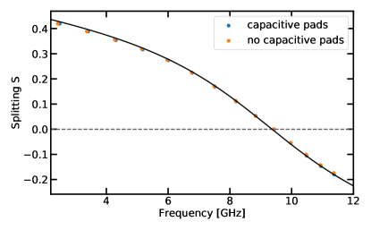
Figure S4: Comparision between the analytical phase shift and the simulated even-odd splitting. The normalized phase shift $\theta_{n}/\pi$ from formula (S46) is in excellent agreement with full ABCD simulations of sample B (dots), confirming also a very small effect of the coupling pads to the output ports.

In the infinite system, the phase shift $\theta$ becomes a continuous function of frequency $\omega$. It vanishes at the renormalized frequency

$$\omega_{J}^{*}=\frac{1}{\sqrt{L^{*}(C_{\text{J}}+C_{\text{sh}})}}$$ (S53)

of the weak link, as can be seen as follows. When $\theta=0$, Eq. (S46) can be rewritten as

$$\cot k=\frac{\lambda+1}{(\lambda-1)X}.$$ (S54)

From the definition of $X$ follows that $\cot k=(X^{2}-1)/2X$, and furthermore, that

$$\frac{X^{2}-1}{2}=2\frac{1-LC\omega^{2}}{LC_{\text{g}}\omega^{2}}-1.$$ (S55)

Using the definition (S44) of $\lambda$ and that of $C_{\Sigma}$, we reduce Eq. (S54) to

$$\frac{1-LC\omega^{2}}{LC_{\text{g}}\omega^{2}}=\frac{1-LC\omega^{2}}{\omega^{2}L[2(C_{\text{J}}+C_{\text{sh}})+C_{\text{g}}]-2L/L^{*}}$$ (S56)

implying that

$$\omega^{2}(C_{J}+C_{\text{sh}})-1/L^{*}=0$$ (S57)

and hence $\omega=1/\sqrt{L^{*}(C_{\text{J}}+C_{\text{sh}})}\equiv\omega_{\text{J}}^{*}$.

.8 Supplementary Note 8: Fitting the experimental splittings

We present in Supplementary Figure S5 the frequency-dependent splittings extracted from the analysis of the even-odd mode pairs (see Supplementary Figure S3), shown as dots for our three samples and various temperatures. Each of this data set is then fitted to the analytical formula (S46), $L^{*}(T)$, or equivalently $E_{\text{J}}^{*}(T)$ being the fitting parameter. The range of investigated temperature is restricted below 130 mK, since at too high temperatures, thermal fluctuations are so strong that the SCHA treatment breaks down. We find in Supplementary Figure S5 that the lineshape of the splitting is well reproduced by our calculations. The location of the zero of the splitting also allows to extract the value of the renormalized frequency $\omega_{\text{J}}^{*}$ of the small junction, a key quantity that is discussed in detail in the main text.

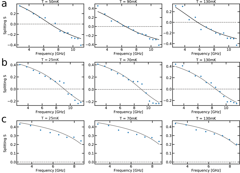
Figure S5: Analysis of the experimental even-odd splitting. The extracted experimental splitting are shown as dots for our three samples (a is for sample A, b is for sample 375 and c is for sample 450) and various temperatures as indicated. Formula (S46) is fitted (black solid lines), allowing the extraction of the renormalized frequency $\omega_{\text{J}}^{*}$.

.9 Supplementary Note 9: Estimation of the shunting capacitance

To determine a value of the unknown shunting capacitance $C_{\text{sh}}$, we devised an original saturation technique. At high enough power, the fluctuations across the small junction can be so large that $E_{\text{J}}^{*}$ renormalizes to zero, decoupling effectively the dynamics of the two chains, except for the remaining effect of $C_{\text{sh}}$ and $C_{\text{J}}$. We can thus use formula (S45), and since $C_{\text{J}}$ is known by design, one can directly infer $C_{\text{sh}}$ from an analysis of the even-odd splitting at high power. The evolution of the transmission as a function of power, and the resulting splittings are shown in Supplementary Figure S6. From that measurement one can infer that $C_{\text{sh}}$ slightly increases (see Table I in the main text) when the size of the junction is increased, which is the expected behavior.

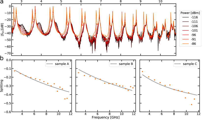
Figure S6: Power scan. Panel a shows the transmission $|S_{21}|$ of sample 300 as a function of the frequency for different power values imposed to the sample. Panel b shows the extracted splitting for our three samples, fitted from Eq. (S45), allowing to extract the shunting capacitance $C_{\text{sh}}$.

.10 Supplementary Note 10: Extracting the parameters of the chain

In this section we discuss how the parameters of the chain are extracted. The chains used in our samples are made out of SQUIDs. Consequently, the inductance of the chains are given by :

$$L=\frac{L_{\text{J}_{\text{ch,min}}}}{\sqrt{\cos[2](\Phi_{\text{C}}/\Phi_{0})+d^{2}\sin[2](\Phi_{\text{C}}/\Phi_{0})}}$$ (S58)

with $\Phi_{\text{C}}$ the flux in the SQUID loops and $d$ the asymmetry of the SQUID junctions Puertas Martinez et al. (2019). As we can neglect the effect output port capacitances, the dispersion relation of the even modes is given by (S39), which can be expressed as a function of $\omega$:

$$\omega(k)=\frac{1}{\sqrt{L(\Phi_{\text{C}})C}}\sqrt{\frac{1-\cos(ka)}{1-\cos(ka)+\frac{C_{\text{g}}}{2C}}}$$ (S59)

From Eq. (S58), the free spectral range (namely the energy difference between two consecutive modes) is decreasing when $\Phi_{\text{C}}/\Phi_{0}$ goes to $\pi/2$. This behavior is clearly seen in Supplementary Figure S7. One can also notice the absence of artifacts around $\Phi_{\text{C}}=0$, which means that the chain is homogeneous and relatively exempt of disorder. By doing a two-tone spectroscopy at $\Phi_{\text{C}}=0$, we can measure precisely the dispersion of the even modes up to 14GHz. From Eq. (S59), we find $C_{\text{g}}$ and $L$ for the three sample, $C$ being known by design. This method allows an in-situ determination of the chain parameters.

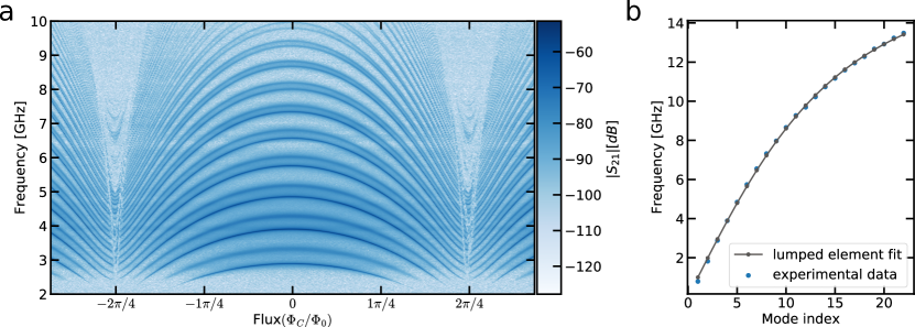
Figure S7: Determination of the chain parameters. Panel a shows the transmission $|S_{21}|$ of sample C as a function of the frequency for different flux in the SQUIDs of the chain. Panel b shows the dispersion relation for the even modes extracted at half flux quantum.

.11 Supplementary Note 11: Perturbative treatment of the non linearity

The perturbative treatment is commonly used in circuit-QED whenever one needs to consider the non-linearity induced by a Josephson junction in a superconducting circuit Nigg et al. (2012); SWeissl et al. (2015). As a first step, the tunnelling energy $E_{\text{J,bare}}(1-\cos\hat{\phi}_{\text{J}})$ is approximated by its harmonic approximation $E_{\text{J,bare}}\hat{\phi}_{\text{J}}^{2}/2$, leading to an effective quadratic Hamiltonian (without any renormalization) $\hat{H}^{\text{lin}}=\sum_{k=0}^{M}{\hbar\omega^{\text{lin}}_{k}\hat{a}^{\dagger}_{k}\hat{a}_{k}}$ and a mode decomposition of the phase fluctuating across the weak link $\hat{\phi}_{\text{J}}=\sum_{k=0}^{M}{\phi^{\text{lin}}_{k}(\hat{a}_{k}^{\dagger}+\hat{a}_{k})}$. The non linearity is then reintroduced at quartic level:

$$\hat{H}\simeq\hat{H}^{\text{lin}}-\frac{E_{\text{J}}}{24}\hat{\phi}_{\text{J}}^{4}.$$ (S60)

This quartic perturbation renormalizes the modes at order $E_{\text{J}}$:

$$\omega_{k}^{*} =\omega_{k}-[K]_{k,k}+\sum_{j\neq k}{[K]_{\text{k,j}}},$$ (S61)

$$K_{k,j} =E_{\text{J}}\left(\frac{\pi}{R_{\text{Q}}}[R]_{0,k}[R]_{0,j}\right)^{2}.$$ (S62)

$[K]$ is known as the Kerr matrix SKrupko et al. (2018). Using this formalism, one can compute the splitting between odd and even modes (see Supplementary Figure S8). Fitting with the phase shift formula (S46), we deduce the renormalized Josephson energy from the Kerr theory $E_{\text{J,Kerr}}^{*}$, which can be compared to the SCHA estimate $E_{\text{J,SCHA}}^{*}$ and the bare value $E_{\text{J,bare}}$. For sample B, we find $E_{\text{J,bare}}=5.61$ GHz, $E_{\text{J,Kerr}}=4.47$ GHz and $E_{\text{J,SCHA}}=3.30$ GHz. The renormalization of $E_{J,\text{bare}}$ from the SCHA acquires a clear non-perturbative character, which the standard Kerr approach is unable to predict quantitatively. This confirms that our device operates in the many-body regime, and cannot be described by standard approaches such as black-box-quantization Nigg et al. (2012).

]

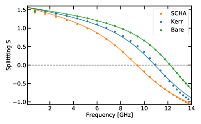
Figure S8: Comparing various quantum approaches of many-body circuits. The even-odd splittings for parameters of sample B are obtained from three numerical approaches (dots): a bare formalism using the fully linearized Josephson Hamiltonian (green), a Kerr approach incorporating the quartic correction (blue), and the self-consistent harmonic approximation taking into account the full cosine form of the potential (orange). Solid lines are the fits from the phase shift formula (S46) allowing to extract the resonance frequency of the junction, and its associated Josephson energy.

References

- Greentree et al. (2006) Andrew D Greentree, Charles Tahan, Jared H Cole, and Lloyd C L Hollenberg, “Quantum phase transitions of light,” Nature Physics 2, 856–861 (2006).
- Carusotto and Ciuti (2013) Iacopo Carusotto and Cristiano Ciuti, “Quantum fluids of light,” Reviews of Modern Physics 85, 299–366 (2013).
- Le Hur et al. (2016) Karyn Le Hur, Loïc Henriet, Alexandru Petrescu, Kirill Plekhanov, Guillaume Roux, and Marco Schiró, “Many-body quantum electrodynamics networks: Non-equilibrium condensed matter physics with light,” Comptes Rendus Physique 17, 808–835 (2016).
- Houck et al. (2012) Andrew A Houck, Hakan E Türeci, and Jens Koch, “On-chip quantum simulation with superconducting circuits,” Nature Physics 8, 292–299 (2012).
- Koch et al. (2007) Jens Koch, Terri M Yu, Jay Gambetta, A A Houck, D I Schuster, J Majer, Alexandre Blais, M H Devoret, S M Girvin, and R J Schoelkopf, “Charge-insensitive qubit design derived from the Cooper pair box,” Physical Review A 76, 042319 (2007).
- Vion et al. (2002) D Vion, A Aassime, A Cottet, P Joyez, H Pothier, C Urbina, D Esteve, and MH Devoret, “Manipulating the quantum state of an electrical circuit,” Science 296, 886–889 (2002).
- Manucharyan et al. (2009) V E Manucharyan, J Koch, L I Glazman, and M H Devoret, “Fluxonium: Single Cooper-Pair Circuit Free of Charge Offsets,” Science 326, 113–116 (2009).
- Weiss (1992) U. Weiss, Quantum Dissipative Systems (World Scientific., 1992).
- Fragner et al. (2008) A Fragner, M Göppl, J M Fink, M Baur, R Bianchetti, P J Leek, A Blais, and A Wallraff, “Resolving Vacuum Fluctuations in an Electrical Circuit by Measuring the Lamb Shift,” Science 322, 1357–1360 (2008).
- Leggett et al. (1987) AJ Leggett, S Chakravarty, AT Dorsey, MPA Fisher, A Garg, and W Zwerger, “Dynamics of the dissipative two-state system,” Reviews of Modern Physics 59, 1 (1987).
- Clarke et al. (1988) J Clarke, AN Cleland, M H Devoret, D Esteve, and JM Martinis, “Quantum-mechanics of a macroscopic variable-The phase difference of a josephson junction,” Science 239, 992–997 (1988).
- Schwartz et al. (1985) D. B. Schwartz, B. Sen, C. N. Archie, and J. E. Lukens, “Quantitative study of the effect of the environment on macroscopic quantum tunneling,” Phys. Rev. Lett. 55, 1547–1550 (1985).
- Zaikin and Panyukov (1986) A. D. Zaikin and S. V. Panyukov, “Lifetime of macroscopic current states,” JETP Lett. 43, 670 (1986).
- Panyukov and Zaikin (1988) S. V. Panyukov and A. D. Zaikin, “Quantum fluctuations and the current-phase relation in josephson junctions and squids,” Physica B: Condensed Matter 152, 162 (1988).
- Nigg et al. (2012) Simon E. Nigg, Hanhee Paik, Brian Vlastakis, Gerhard Kirchmair, S. Shankar, Luigi Frunzio, M. H. Devoret, R. J. Schoelkopf, and S. M. Girvin, “Black-box superconducting circuit quantization,” Phys. Rev. Lett. 108, 240502 (2012).
- Bourassa et al. (2012) J. Bourassa, F. Beaudoin, Jay M. Gambetta, and A. Blais, “Josephson-junction-embedded transmission-line resonators: From Kerr medium to in-line transmon,” Physical Review A - Atomic, Molecular, and Optical Physics 86, 1–13 (2012), arXiv:1204.2237 .
- Weissl et al. (2015a) T Weissl, B Küng, E Dumur, A K Feofanov, I Matei, C Naud, O Buisson, F W J Hekking, and W Guichard, “Kerr coefficients of plasma resonances in Josephson junction chains,” Physical Review B 92, 104508–10 (2015a).
- Puertas Martinez et al. (2019) Javier Puertas Martinez, Sebastien Leger, Nicolas Gheeraert, Remy Dassonneville, Luca Planat, Farshad Foroughi, Yuriy Krupko, Olivier Buisson, Cécile Naud, Wiebke Hasch-Guichard, Serge Florens, Izak Snyman, and Nicolas Roch, “A tunable Josephson platform to explore many-body quantum optics in circuit-QED,” npj Quantum Information , 1–8 (2019).
- Schmid (1983) Albert Schmid, “Diffusion and Localization in a Dissipative Quantum System,” Physical Review Letters 51, 1506–1509 (1983).
- Bulgadaev (1984) S.A. Bulgadaev, “Phase diagram of a dissipative quantum system,” jetpletters.ac.ru (1984).
- Murani et al. (2019) Anil Murani, Nicolas Bourlet, Hélène le Sueur, Fabien Portier, Carles Altimiras, Daniel Esteve, Hermann Grabert, Jürgen Stockburger, and Philippe Joyez, “Absence of a dissipative quantum phase transition in Josephson junctions,” arXiv.org (2019), 1905.01161v1 .
- Schön and Zaikin (1990) Gerd Schön and A D Zaikin, “Quantum coherent effects, phase transitions, and the dissipative dynamics of ultra small tunnel junctions,” Physics Reports 198, 237–412 (1990).
- Hekking and Glazman (1997) F W J Hekking and L I Glazman, “Quantum fluctuations in the equilibrium state of a thin superconducting loop,” Phys Rev B 55, 6551–6558 (1997).
- Kuzmin et al. (1991) L S Kuzmin, Yu V Nazarov, D B Haviland, P Delsing, and T Claeson, “Coulomb blockade and incoherent tunneling of Cooper pairs in ultrasmall junctions affected by strong quantum fluctuations,” Physical Review Letters 67, 1161–1164 (1991).
- Huard et al. (2007) B. Huard, H. Pothier, D. Esteve, and K. E. Nagaev, “Electron heating in metallic resistors at sub-Kelvin temperature,” Physical Review B - Condensed Matter and Materials Physics 76, 1–9 (2007).
- Manucharyan (2012) Vladimir Eduardovich Manucharyan, “Superinductance,” Thesis (2012).
- Masluk et al. (2012) Nicholas Masluk, Ioan Pop, Archana Kamal, Zlatko Minev, and Michel Devoret, “Microwave Characterization of Josephson Junction Arrays: Implementing a Low Loss Superinductance,” Physical Review Letters 109, 137002 (2012).
- Bell et al. (2012) M. Bell, I. Sadovskyy, L. Ioffe, A. Kitaev, and M. Gershenson, “Quantum Superinductor with Tunable Nonlinearity,” Physical Review Letters 109, 137003 (2012).
- Maleeva et al. (2018) N. Maleeva, L. Grünhaupt, T. Klein, F. Levy-Bertrand, O. Dupre, M. Calvo, F. Valenti, P. Winkel, F. Friedrich, W. Wernsdorfer, A. V. Ustinov, H. Rotzinger, A. Monfardini, M. V. Fistul, and I. M. Pop, “Circuit quantum electrodynamics of granular aluminum resonators,” Nature Communications 9, 1–7 (2018).
- Ingold and Nazarov (1992) Gert-Ludwig Ingold and Yu V Nazarov, “Charge Tunneling Rates in Ultrasmall Junctions,” in Single Charge Tunneling (Springer, Boston, MA, Boston, MA, 1992) pp. 21–107.
- Corlevi et al. (2006) S Corlevi, W Guichard, FWJ Hekking, and DB Haviland, “Phase-charge duality of a Josephson junction in a fluctuating electromagnetic environment,” Phys Rev Lett 97, 96802 (2006).
- Ergül et al. (2013) Adem Ergül, Jack Lidmar, Jan Johansson, Yağız Azizoğlu, David Schaeffer, and David B Haviland, “Localizing quantum phase slips in one-dimensional josephson junction chains,” New Journal of Physics 15, 095014 (2013).
- Weissl et al. (2015b) T Weissl, G Rastelli, I Matei, I M Pop, O Buisson, F W J Hekking, and W Guichard, “Bloch band dynamics of a Josephson junction in an inductive environment,” Physical Review B 91, 014507–9 (2015b).
- Wallraff et al. (2004) A Wallraff, DI Schuster, A Blais, L Frunzio, RS Huang, J Majer, S Kumar, SM Girvin, and RJ Schoelkopf, “Strong coupling of a single photon to a superconducting qubit using circuit quantum electrodynamics,” Nature 431, 162–166 (2004).
- Hoi et al. (2015) I C Hoi, A F Kockum, L Tornberg, A Pourkabirian, G Johansson, P Delsing, and C M Wilson, “Probing the quantum vacuum with an artificial atom in front of a mirror,” Nature Physics , 1–5 (2015).
- Silveri et al. (2019) Matti Silveri, Shumpei Masuda, Vasilii Sevriuk, Kuan Y. Tan, Máté Jenei, Eric Hyyppä, Fabian Hassler, Matti Partanen, Jan Goetz, Russell E. Lake, Leif Grönberg, and Mikko Möttönen, “Broadband Lamb shift in an engineered quantum system,” Nature Physics , 1–8 (2019).
- Wen et al. (2019) P Y Wen, K T Lin, A F Kockum, B Suri, H Ian, J C Chen, S Y Mao, C C Chiu, P Delsing, F Nori, G D Lin, and I C Hoi, “Large collective Lamb shift of two distant superconducting artificial atoms,” arXiv.org (2019), 1904.12473 .
- Forn-Díaz et al. (2018) P. Forn-Díaz, L. Lamata, E. Rico, J. Kono, and E. Solano, “ Ultrastrong coupling regimes of light-matter interaction,” arXiv.org (2018), 1804.09275 .
- Kockum et al. (2019) Anton Frisk Kockum, Adam Miranowicz, Simone De Liberato, Salvatore Savasta, and Franco Nori, “Ultrastrong coupling between light and matter,” Nature Reviews Physics , 1–22 (2019).
- Rolland et al. (2019) C Rolland, A Peugeot, S Dambach, M Westig, B Kubala, Y Mukharsky, C Altimiras, H le Sueur, P Joyez, D Vion, P Roche, D Esteve, J Ankerhold, and F Portier, “Antibunched Photons Emitted by a dc-Biased Josephson Junction,” Physical Review Letters 122, 186804 (2019).
- Forn-Díaz et al. (2017) P Forn-Díaz, J J Garcia-Ripoll, B Peropadre, J L Orgiazzi, M A Yurtalan, R Belyansky, C M Wilson, and A Lupaşcu, “Ultrastrong coupling of a single artificial atom to an electromagnetic continuum in the nonperturbative regime,” Nature Physics 13, 39–43 (2017).
- Magazzù et al. (2018) L Magazzù, P Díaz, R Belyansky, J L Orgiazzi, M A Yurtalan, M R Otto, A Lupaşcu, C M Wilson, and M Grifoni, “Probing the strongly driven spin-boson model in a superconducting quantum circuit,” Nature Communications 9, 1403 (2018).
- Garcia-Ripoll et al. (2015) J J Garcia-Ripoll, B Peropadre, and S De Liberato, “Light-matter decoupling and term detection in superconducting circuits,” Scientific Reports 5, srep16055 (2015).
- Malekakhlagh et al. (2017) Moein Malekakhlagh, Alexandru Petrescu, and Hakan E Türeci, “Cutoff-Free Circuit Quantum Electrodynamics,” Physical Review Letters 119, 073601–6 (2017).
- Gely et al. (2017) Mario F Gely, Adrian Parra-Rodriguez, Daniel Bothner, Ya M Blanter, Sal J Bosman, Enrique Solano, and Gary A Steele, “Convergence of the multimode quantum Rabi model of circuit quantum electrodynamics,” Physical Review B 95, 245115–5 (2017).
- Parra-Rodriguez et al. (2018) A Parra-Rodriguez, E Rico, E Solano, and I L Egusquiza, “Quantum networks in divergence-free circuit QED,” Quantum Science and Technology 3, 024012 (2018).
- Gely et al. (2018) Mario F Gely, Gary A Steele, and Daniel Bothner, “Nature of the Lamb shift in weakly anharmonic atoms: From normal-mode splitting to quantum fluctuations,” Physical Review A 98, 053808 (2018).
- Kuzmin et al. (2019) Roman Kuzmin, Nitish Mehta, Nicholas Grabon, Raymond Mencia, and Vladimir E Manucharyan, “Superstrong coupling in circuit quantum electrodynamics,” npj Quantum Information , 1–6 (2019).
- Pozar (2009) David M Pozar, Microwave engineering (John Wiley & Sons, 2009).
- Kampf and Schön (1987) Arno Kampf and Gerd Schön, “Quantum effects and the dissipation by quasiparticle tunneling in arrays of josephson junctions,” Phys. Rev. B 36, 3651–3660 (1987).
- Chakravarty et al. (1988) Sudip Chakravarty, Gert-Ludwig Ingold, Steven Kivelson, and Gergely Zimanyi, “Quantum statistical mechanics of an array of resistively shunted josephson junctions,” Phys. Rev. B 37, 3283–3294 (1988).
- Joyez (2013) Philippe Joyez, “Self-Consistent Dynamics of a Josephson Junction in the Presence of an Arbitrary Environment,” Physical Review Letters 110, 312–5 (2013).
- Garcia-Ripoll et al. (2008) Juan Jose Garcia-Ripoll, Enrique Solano, and Miguel Angel Martin-Delgado, “Quantum simulation of Anderson and Kondo lattices with superconducting qubits,” Physical Review B 77, 024522 (2008).
- Le Hur (2012) K Le Hur, “Kondo resonance of a microwave photon,” Physical Review B 85, 140506 (2012).
- Goldstein et al. (2013) Moshe Goldstein, Michel H Devoret, Manuel Houzet, and Leonid I Glazman, “Inelastic Microwave Photon Scattering off a Quantum Impurity in a Josephson-Junction Array,” Physical Review Letters 110, 017002 (2013).
- Peropadre et al. (2013) B Peropadre, D Zueco, D Porras, and J García-Ripoll, “Nonequilibrium and Nonperturbative Dynamics of Ultrastrong Coupling in Open Lines,” Physical Review Letters 111, 243602 (2013).
- Snyman and Florens (2015) I Snyman and S Florens, “Robust Josephson-Kondo screening cloud in circuit quantum electrodynamics,” Physical Review B 92, 085131 (2015).
- Gheeraert et al. (2017) N Gheeraert, S Bera, and S Florens, “Spontaneous emission of Schrödinger cats in a waveguide at ultrastrong coupling,” New Journal of Physics 19, 023036 (2017).
- Gheeraert et al. (2018) Nicolas Gheeraert, Xin H H Zhang, Théo Sépulcre, Soumya Bera, Nicolas Roch, Harold U Baranger, and Serge Florens, “Particle production in ultrastrong-coupling waveguide QED,” Physical Review A 98, 043816 (2018).

References

- Joyez (2013) P. Joyez, Physical Review Letters 110, 312 (2013).
- Puertas Martinez et al. (2019) J. Puertas Martinez, S. Leger, N. Gheeraert, R. Dassonneville, L. Planat, F. Foroughi, Y. Krupko, O. Buisson, C. Naud, W. Hasch-Guichard, S. Florens, I. Snyman, and N. Roch, npj Quantum Information , 1 (2019).
- Pozar (2009) D. M. Pozar, Microwave engineering (John Wiley & Sons, 2009).
- Nigg et al. (2012) S. E. Nigg, H. Paik, B. Vlastakis, G. Kirchmair, S. Shankar, L. Frunzio, M. H. Devoret, R. J. Schoelkopf, and S. M. Girvin, Physical Review Letters 108, 260 (2012).
- SWeissl et al. (2015) T. Weissl, B. Küng, E. Dumur, A. K. Feofanov, I. Matei, C. Naud, O. Buisson, F. W. J. Hekking, and W. Guichard, Physical Review B 92, 104508 (2015).
- SKrupko et al. (2018) Y. Krupko, V. D. Nguyen, T. Weissl, E. Dumur, J. Puertas, R. Dassonneville, C. Naud, F. W. J. Hekking, D. M. Basko, O. Buisson, N. Roch, and W. Hasch-Guichard, Phys Rev B 98, 094516 (2018).